1. Introduction
Adaptive meshing is a fundamental component of adaptive finite element methods. This includes refining and coarsening meshes locally [
1,
2]. As the mesh is enriched through the refinement process, the solution on a given mesh provides an accurate starting iterate for the next mesh. Frequently, it is needed not only to enrich the mesh but also to coarsen it by some derefinement or coarsening strategy [
3,
4] in such a way that the nodes are located in the places where it is necessary for a more accurate solution while the number of unknowns remains bound. Mesh coarsening and mesh refinement are usually combined to provide a flexible approach for the adaptation of time-dependent problems [
5].
In the context of adaptive finite element methods, both in two and three dimensions, longest-edge bisection-based algorithms have been largely studied in the last years [
6,
7,
8]. These algorithms guarantee the construction of high-quality triangulations [
9,
10], assuring the maximum angle condition [
11] and the non-degeneracy of the obtained meshes [
10]. Non-degeneracy of the meshes means that the minimum angle generated is bounded away from zero, and it is closely related to the finite number of similarly different triangles or tetrahedra generated. Further, some longest-edge bisection-based partitions show a mesh quality improvement property, meaning that the generated meshes not only do not degenerate but also present better quality than the previously obtained mesh as the refinement is applied.
For coarsening a refined mesh, we may consider different approaches, such as removing nodes, swapping edges, or amplifying elements [
2]. Here we study the shortest-edge duplication of a triangle as a simple procedure to be applied to those triangles for coarsening a triangular mesh that has been obtained by the iterative application of local refinements based on longest-edge bisection. This method shows to be effective at coarsening meshes while improving the smallest angle. On the other hand, if it is desired to maintain the resolution of the mesh while improving the smallest angles, the method can be combined with a local refinement strategy to improve high-order mesh quality while maintaining sufficient resolution, for example, by the self-similar refinement scheme [
2,
12], albeit this issue will not be tackled in this paper. It should be underlined, however, that there have been recent approaches, such as the
-adaptivity, which are able to address this problem [
13].
Our goal in the paper is to study the metric properties of the shortest-edge duplication, in the sequel SE duplication, of a triangle. To this end, we will employ the results of hyperbolic geometry and particularly the Poincare half-plane model, which has demonstrated its utility in similar triangle partitions [
14,
15].
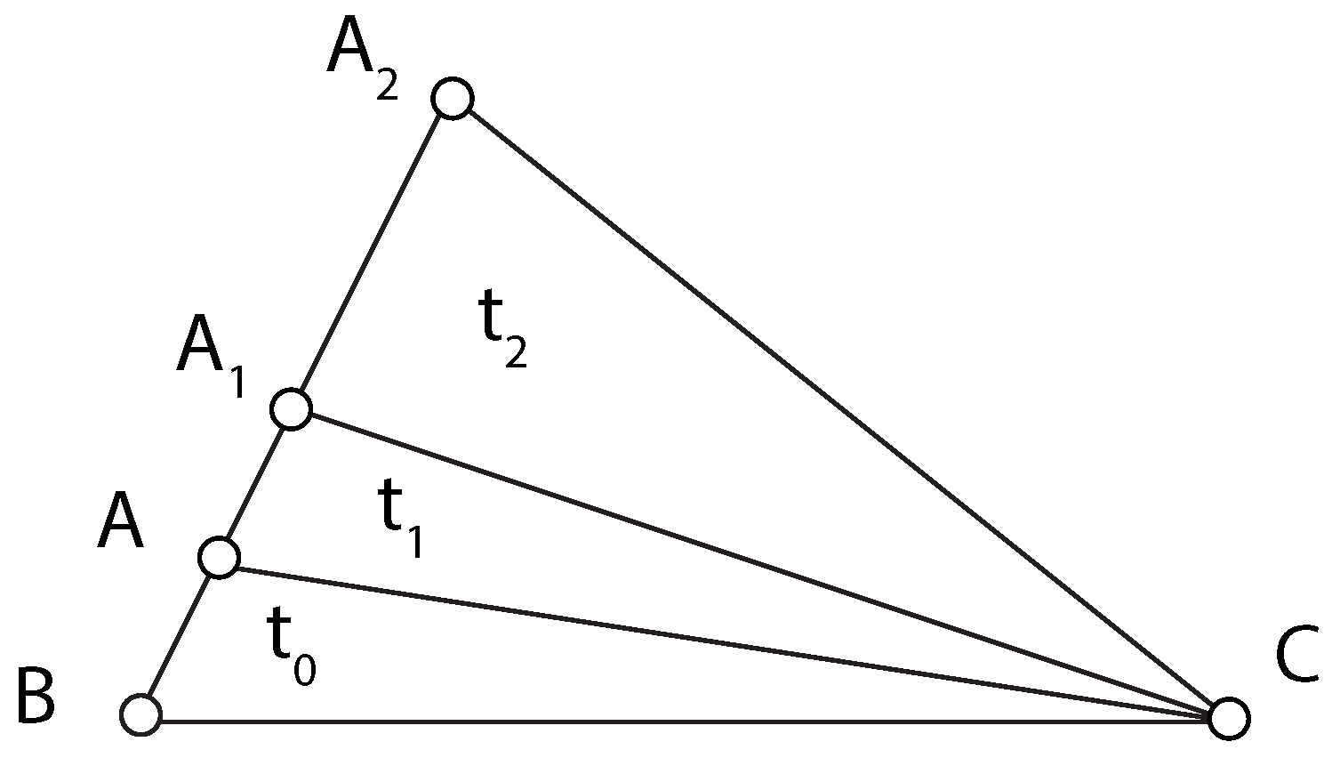
Given an initial triangle, a new triangle is obtained by doubling the shortest edge, maintaining the longest edge as unaltered. The SE duplication will be explicitly set up in the next definition.
Definition 1. Let denote triangle with vertices A, B and C. Let us assume that the shortest edge of is edge , while the longest one is edge . Then, the SE SE duplication of is , where .
Notice that the SE duplication is a transformation of triangles that may be applied recursively. For example, and continuing with the triangle in Definition 1, if the shortest-edge of triangle
is
, and the longest one is
, the SE duplication of
is triangle
, where
. See
Figure 1.
It is clear that by the SE duplication of a triangle, the two shortest edges of the triangle increase, while the longest edge remains unaltered.
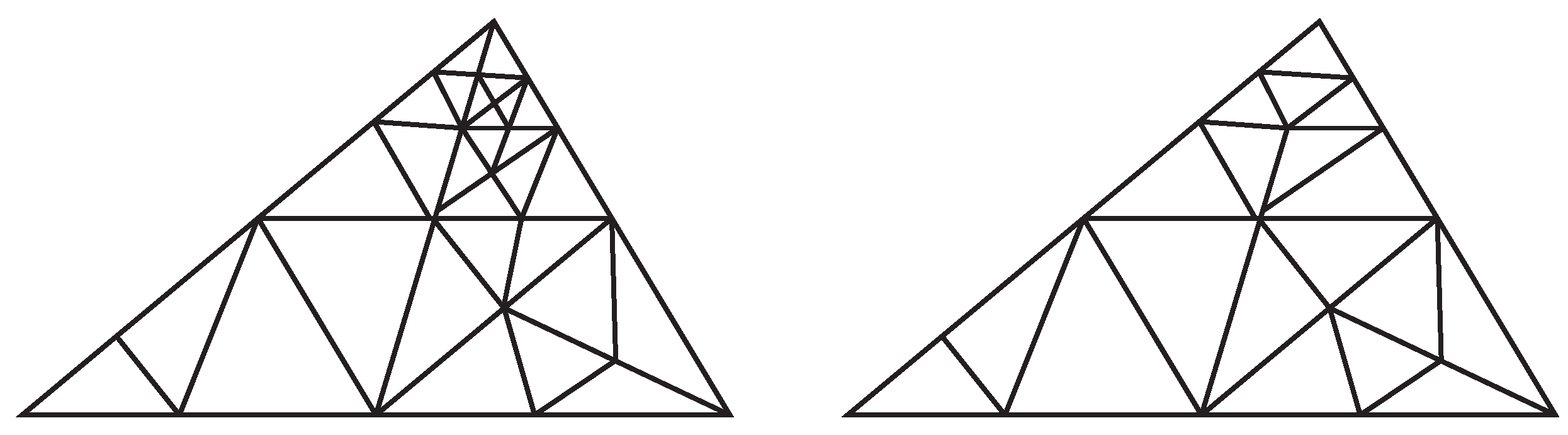
Let
be a locally refined triangular mesh obtained by a longest-edge bisection-based refinement. One could apply the SE duplication of some triangles in order to coarsen the mesh. This procedure consists of locally changing a triangle by SE duplication. As a matter of example,
Figure 2 shows the application of SE duplication to a refined mesh obtained by the longest-edge bisection so that a derefined mesh appears.
2. Normalised Region for Triangles and Piecewise Function for the SE Duplication
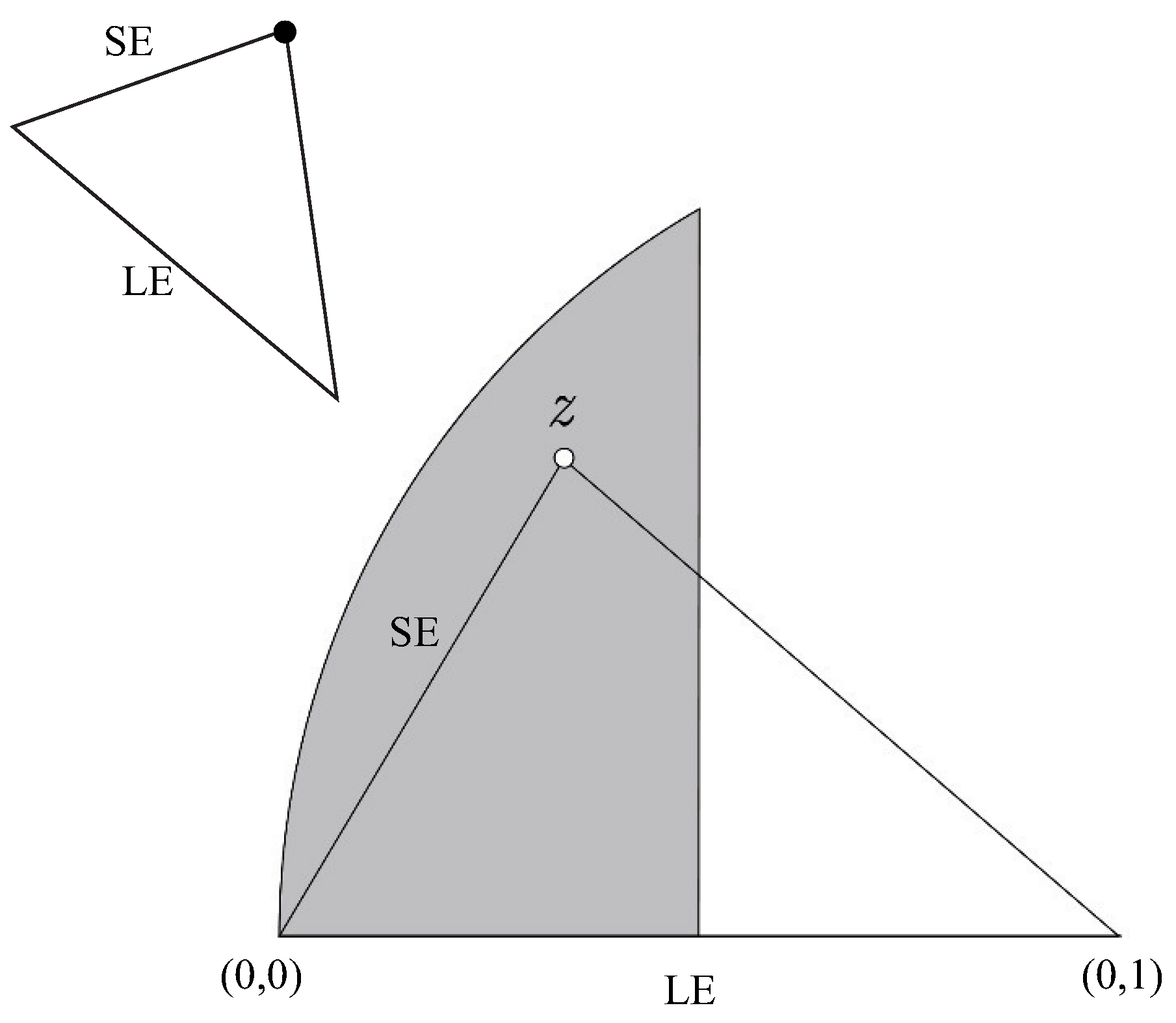
For any arbitrary triangle, a similar triangle can be found by performing suitable symmetries, scaling, translations and rotations such that the normalised triangle has the longest edge with vertices
and
, and the opposite vertex,
z, in the upper plane at the left of the vertical line
; that is, with the shortest edge to the left with vertices
and
z [
12]. Using this procedure, all similar triangles are represented by a unique complex number
, where
is the set of the complex plane
.
is called the space of triangular shapes. See
Figure 3, where
is in grey.
For any point
, let
be its image in
by the shortest-edge duplication transformation.
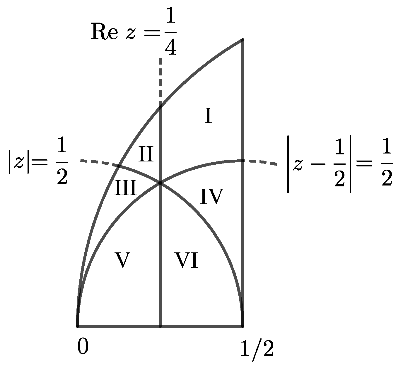
is a piecewise function that depends on the location of
z in
. Explicitly, function
is defined as follows, depending on which subregion point
z is in according to the subregions in
Figure 4.
Figure 4 shows the subdomains in
needed to define function
.
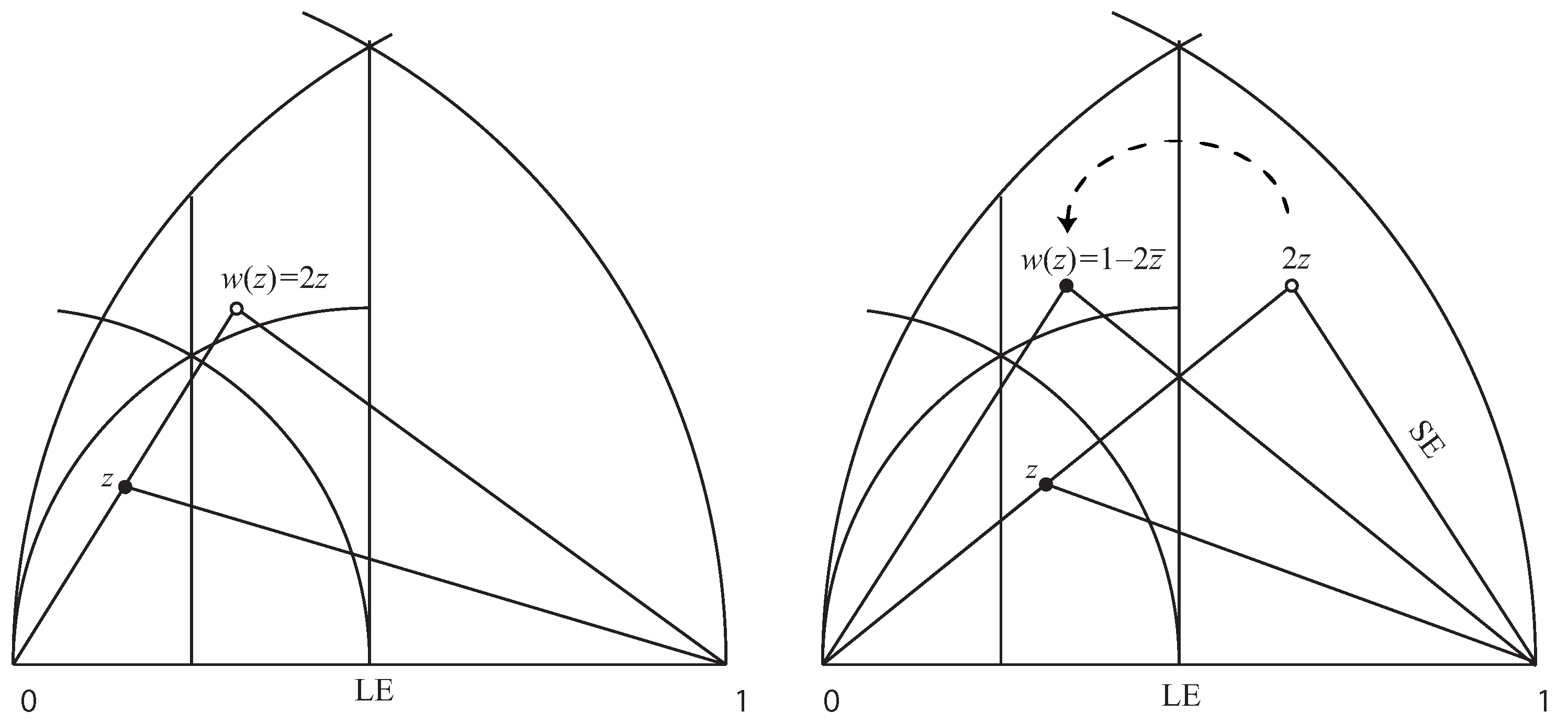
The values of function
w, depending on the position of point
z in each sub-region, may be easily deduced. As a matter of example,
Figure 5 shows the definition of function
for
z in the first two lower subregions of the space of triangular shapes. Similar figures may be found for the other subregions. In
Figure 5 right,
, while in
Figure 5 left,
in order to normalise the triangle to have its shortest edge on the left side, so that
belongs to
.
Using hyperbolic geometry, such as the Poincare half-plane model, see [
14,
15,
16,
17], the circumferences and straight lines in the definition of the piecewise function
w are orthogonal to
and, therefore, are geodesics in the Poincare half-plane. The expressions for function
w are isometries in the half-plane hyperbolic model because they have the form
or
with real coefficients
. Function
w is invariant with respect to the inversion of the circumferences
and
, and under symmetry with respect to the straight line
. We recall here the expression of these transformations in [
18]. Let
K be an arbitrary circle with centre
q and radius
R. Then the inversion in
K, written
, is equal to
In particular, for , circle , we have , while for , circle , we have .
On the other hand, ff is a line in the complex plane such that is the reflection of in the given line, then . In particular, for the straight line L with equation , the expression of the reflection in line L, say , is .
Theorem 1. Function w is invariant with respect to the inversion of the two circumferences, and , and under symmetry with respect to the straight line that appears in its definition.
Proof. The proof follows easily by checking that
Similarly, for inversions
, with
, it holds, in closed form, that
where
J represents any subregion in the definition of function
w. □
If
and
are such that
, then the hyperbolic distance
d between
and
,
, is
On the other hand, if
, then
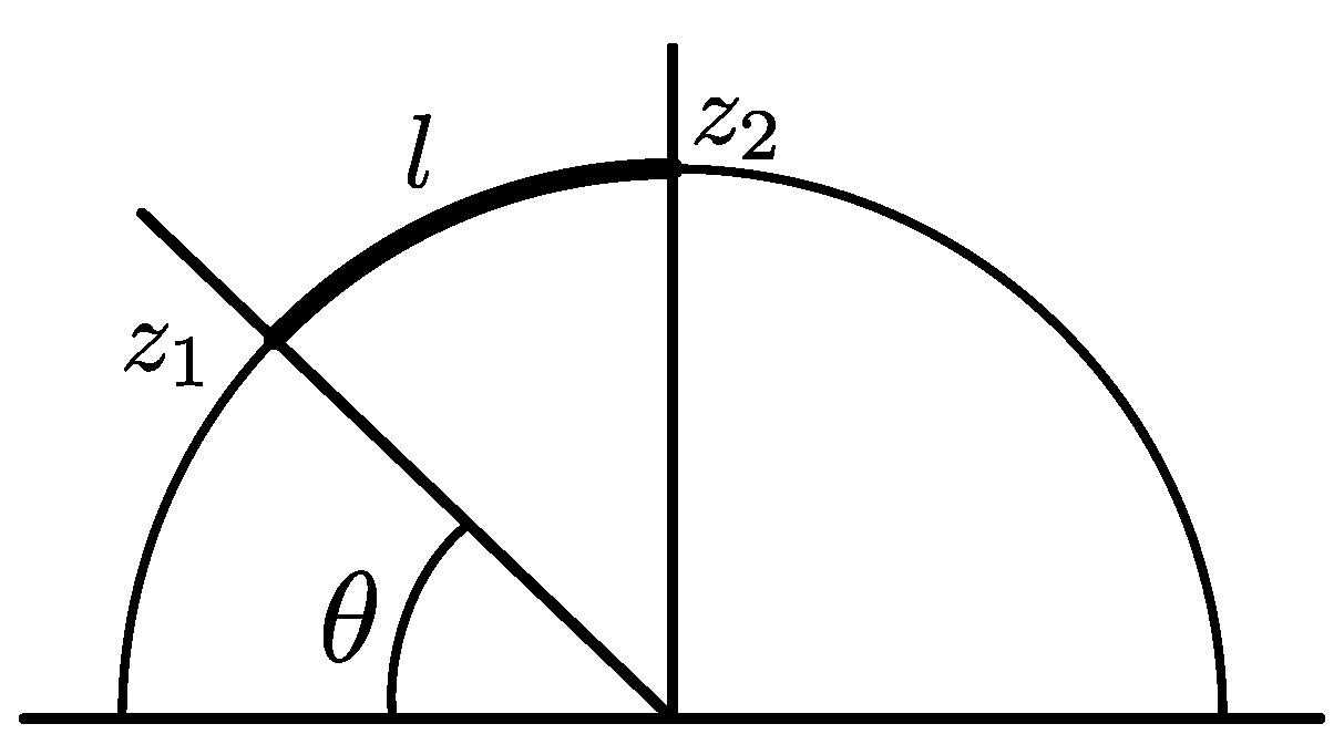
Let
and
be points in a geodesic circumference, and
be the upper point located over the centre of the circumference, the hyperbolic length of the segment in the geodesic from
to
, say
l, verifies
where
is the difference between
and the central angle is determined by the segment from
to
over the geodesic. See
Figure 6.
Definition 2. A region is called a closed region for SE duplication if .
Lemma 1 (non-increasing property). If , then .
Proof. Let us first assume that and are in a region with the same definition of w, then . This may be checked easily and also follows because w is an isometry in .
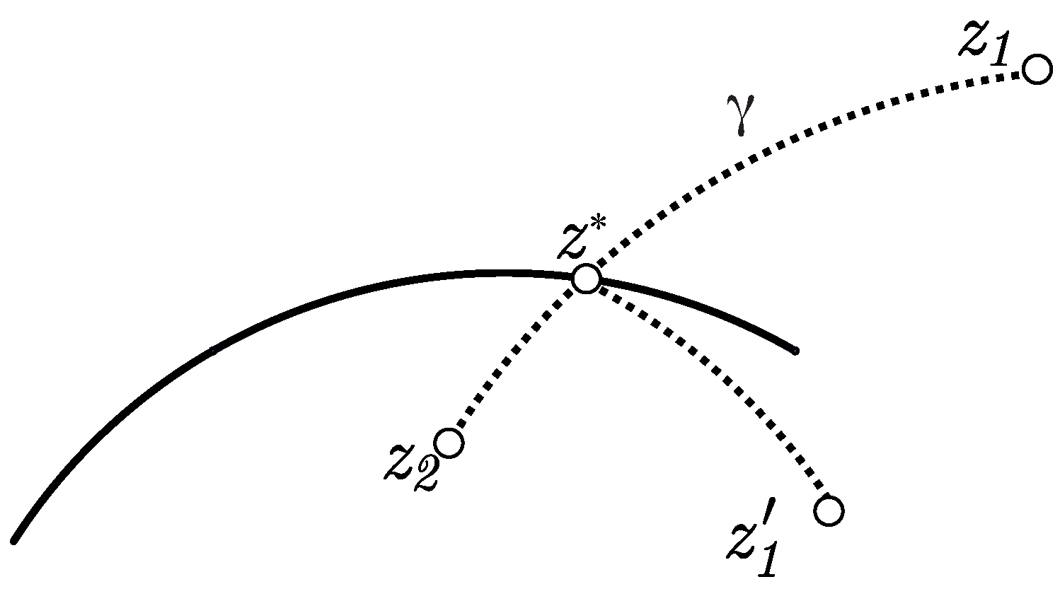
Suppose now that
and
are not in a region with the same definition of
w.
and
may be in two regions sharing a common boundary. In this case, there is
in the region of
with
because of the symmetry of
w with respect to the boundary. Let
be the geodesic line that joins
and
.
intersects the boundary at a point, say
. Then, since points
,
and
are in the same geodesic,
. Further,
because
and
are symmetrical points with respect to the boundary containing
. See
Figure 7.
Therefore, by the triangular inequality,
Thus, .
If, and are in different regions not sharing a common boundary, we may apply the previous process to bring both and into the same region and the proof is finished. □
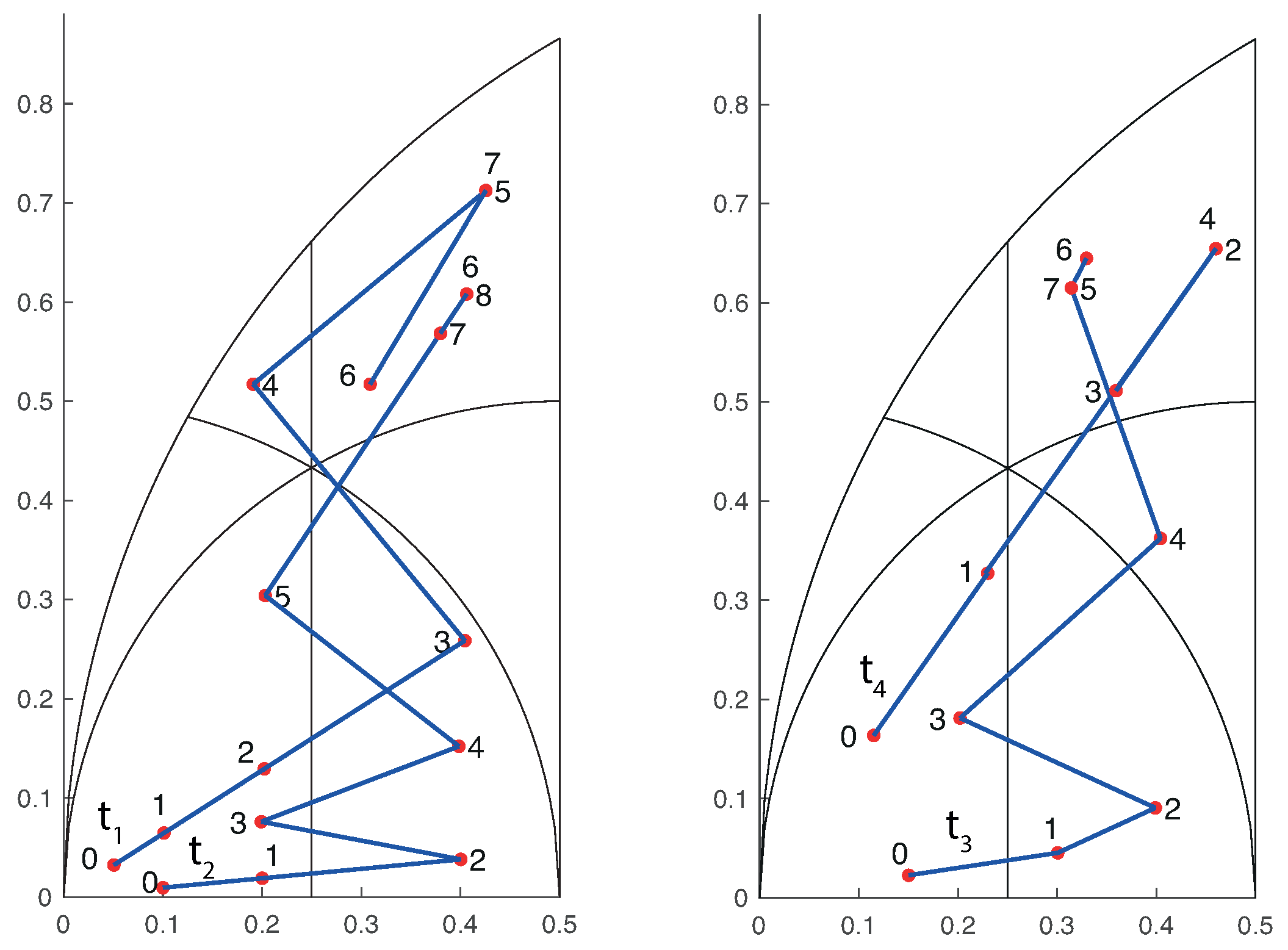
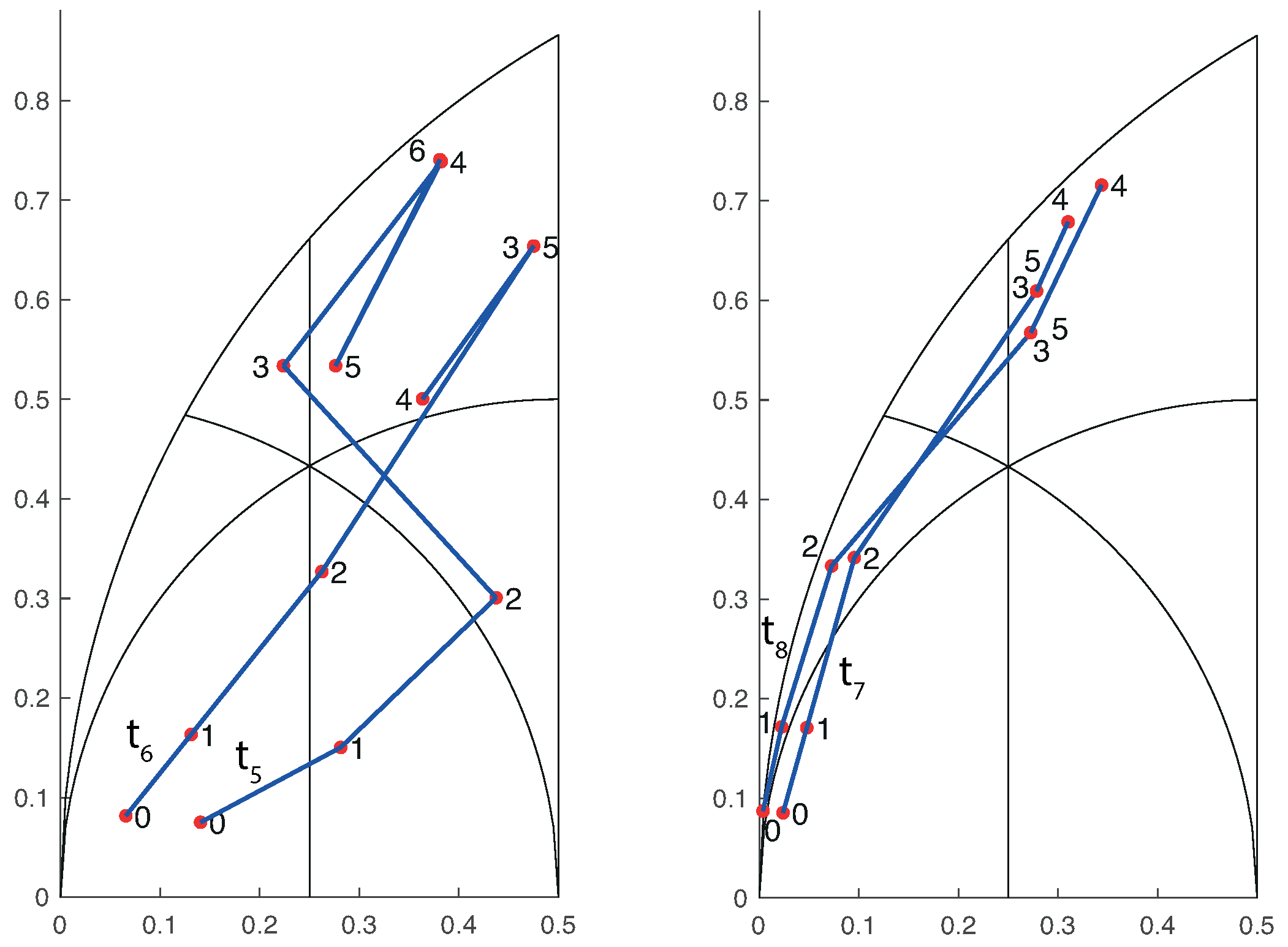
Definition 3. Let z be in Σ. The orbit of z by the SE duplication, , is the set as , where , and .
For
,
, since
. Other fixed points for
w are
and
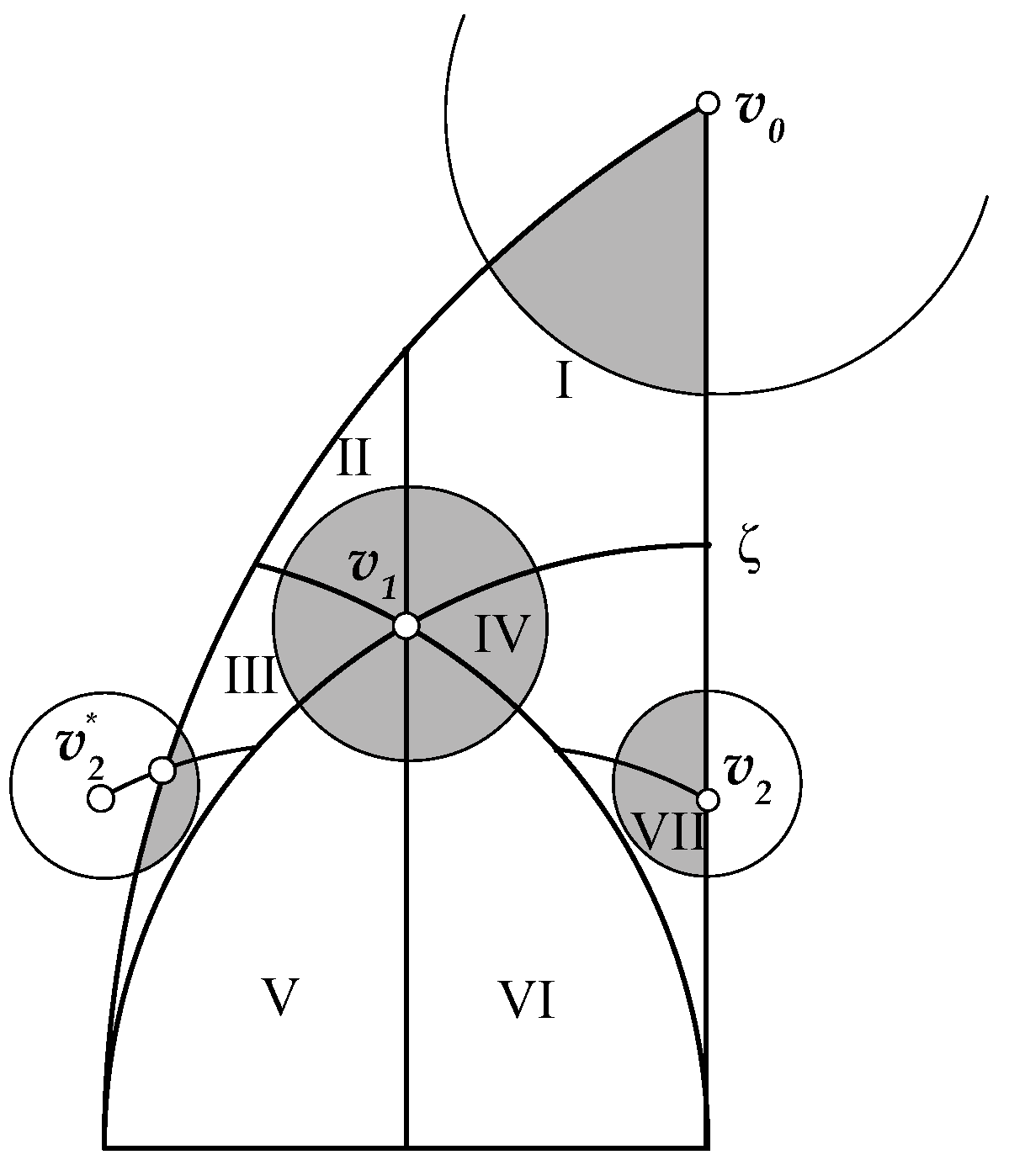
. In sub-region
I, as denoted in
Figure 8,
, which is an inversion with respect to the circumference of equation
, or
. Therefore, for
z in the arc of that circumference which is in region
I,
. It may be easily verified that these are the only fixed points for
.
Notice that although
is another fixed point, that triangle is invalid and does not belong to the space of triangular shapes
where it is required
. Further, it follows that for
,
. For example, for
, which corresponds to the equilateral triangle, then
, where
.
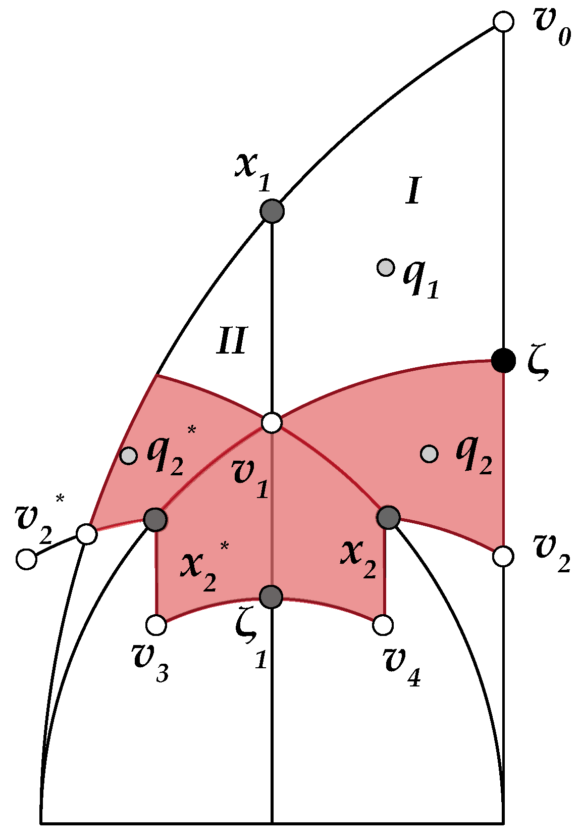
In order to prove that the orbit for any point
z is finite, we will use the division of the normalised region is shown in
Figure 8. We consider the sets
, with
, where
. It is clear that
. These sets are the coloured subsets in
Figure 8. The points labelled in the figure are
,
and
are pre-images of
. Similarly,
,
,
,
, and
. Further,
is the pre-image of
in region
; that is,
, while
.
Lemma 2. is a closed region. Further, if , then
Proof. Let . If , is an inversion with respect to the circumference of equation , then . Therefore, for , . Further, by construction, , with , so for . Finally, by the symmetry of function w about line , then for , , and, therefore, for . □
The argument of the last lemma may be applied recursively, considering each of the pre-images of the last sets by , with . In that way, since the pre-images of the lowest vertices considered tend to the horizontal line , it follows that , . This fact will also be shown experimentally by a Monte Carlo experiment later.
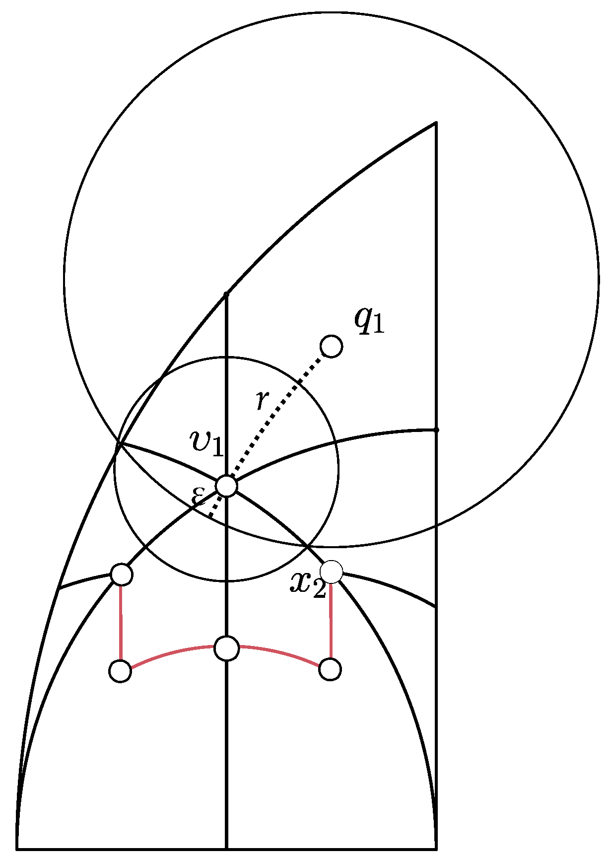
Lemma 3. There is such that for every such that the hyperbolic distance to any of the points , , or is less than or equal to then
Proof. Notice that
may be chosen such that every hyperbolic circle with centre
,
,
or
and radius
intersects only the geodesic lines defining
w that pass through their centres, as
Figure 9 shows.
Let us first suppose that with . In that case, so
On the other hand, if , , so Finally, if or , then , so it is reduced to the previous case. □
Lemma 4. Let and . Then there exists such that for every with , then
Proof. Let us consider that
is small enough so that the hyperbolic circle with a centre at
and radius
does not intersect with region
. This is possible because
, as it is shown in
Figure 10. With such a
, we may assure that the region of
z such that
is contained in
along with a small hyperbolic circle with its centre at
, so it is inside region
S from Lemma 2. It follows that
□
Lemma 5. Let as in the previous lemma, and . Let K be a compact set contained in the normalised region such that for every it holds that . Then, there exists a value A, where such that for every , .
Proof. Function
is continuous in
K. Since
K is compact, there exists
A, the maximum value of
in
K. By not increasing the distance and since
, then
. In addition, if
,
z is not in region
I, and the inequality between the distances is strict. In particular, this happens for the value of
in where the maximum is attained, where
. □
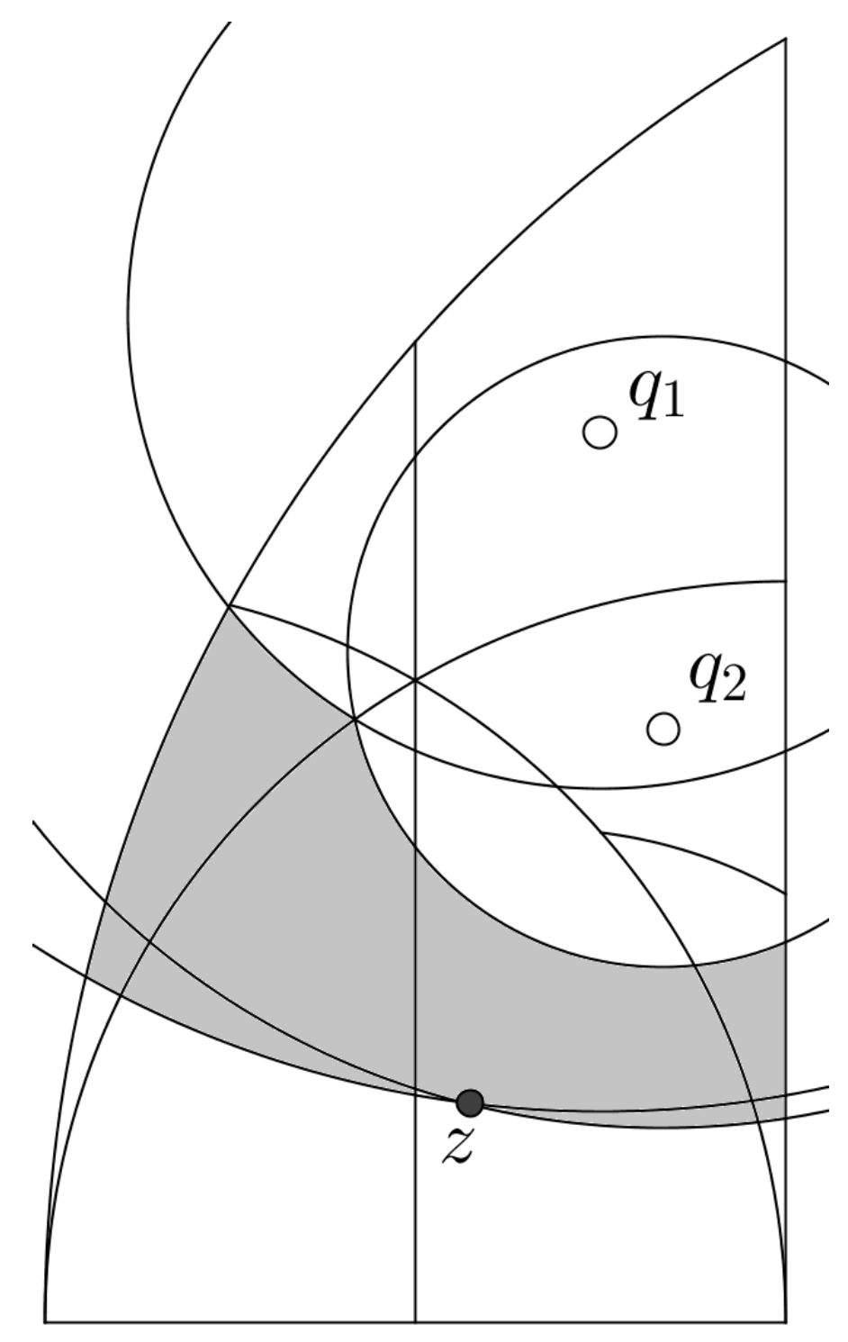
Theorem 2. If , then
Proof. Let
r and
be as in the previous lemmas. If
, then
, by Lemma 5. Let us suppose, therefore, that
. Let
K be the compact set given by the points
such that
with
, and also
with
. In
Figure 11,
K is grey. By Lemma 5, there exists
A such that for every
,
. Therefore,
with
. By the non-increasing property,
. Therefore, either
or the orbit
By iterating this process, the orbit
is described as a finite set and a finite number of finite orbits of points with a distance to
of less than or equal to
. Therefore, by Lemma 4 these orbits are also finite. □
3. Classes of Triangles
Here, we focus on the number of dissimilar triangles that are produced in the SE duplication scheme. Our goal in this section is to study the number of dissimilar triangles so that we can get a classification of the triangles. Let class be the set of triangles for which the SE duplication produces exactly n dissimilar triangles.
We develop a Monte Carlo experiment that can be used to visually represent the classes of triangles according to the number of dissimilar triangles generated.
The process can be described in three phases: (1) Pick a point within the mapping domain defined by the horizontal base and by the two bounding exterior circular arcs. This point
is the apex of a target triangle. (2) Apply SE duplication to the triangle defined by
z and its successors and stop when no new shapes appear. (3) The number of steps until termination defines the number of dissimilar triangles for
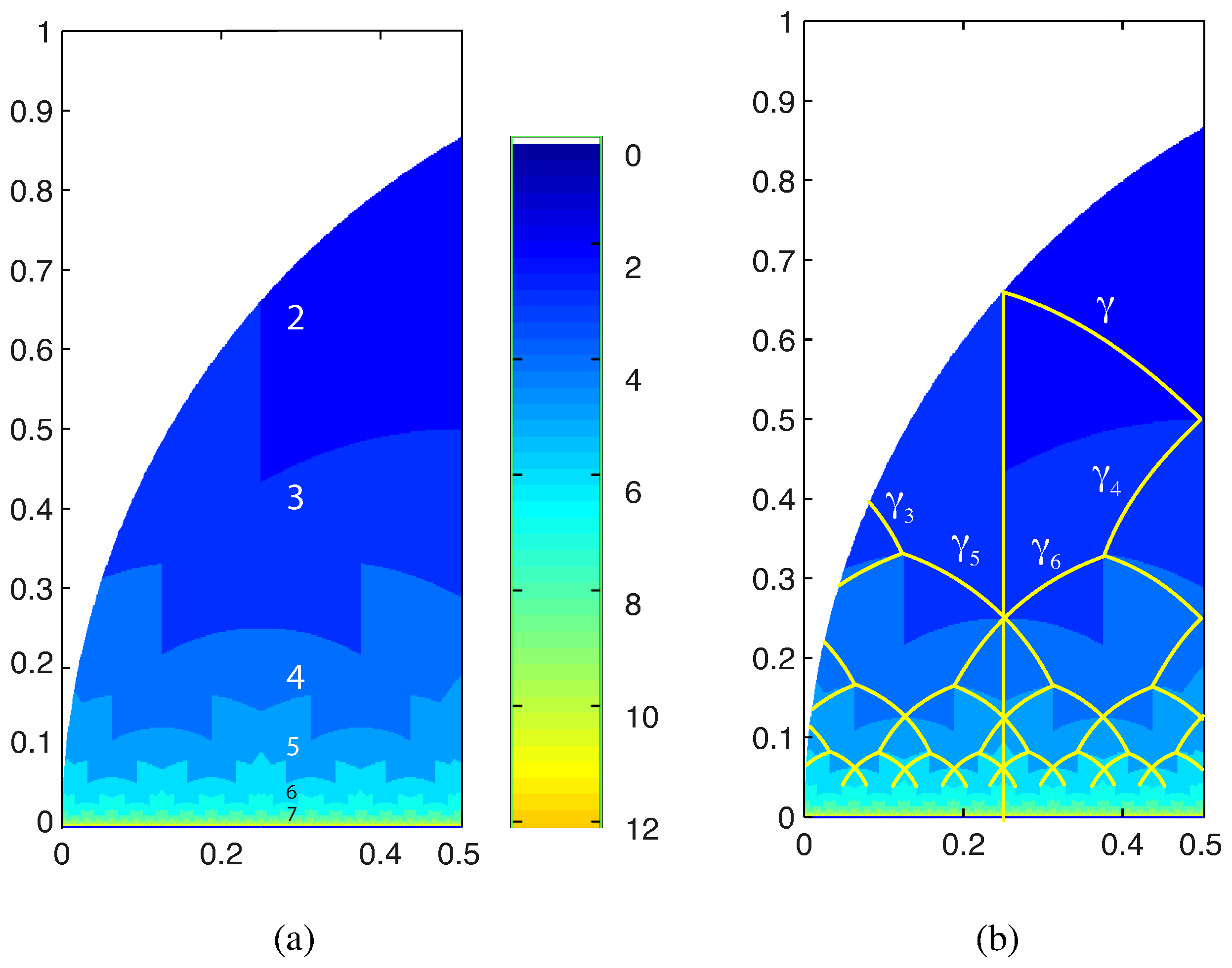
z. This process is recursively applied to a large sample of triangles uniformly over the domain. The output of the experiment is a graph where all of the dissimilar triangles are represented using a colour map to obtain the result in
Figure 12.
Note that the number of dissimilar triangles has been drawn within several coloured regions. For instance, label 2 stands for the two dissimilar triangles and is associated with the targeted triangles within the region above the pair of arcs that intersect on the vertical line of symmetry near the point . Label 3 is in the region below for the 3 dissimilar triangles. A graph is then constructed in this manner that fills a completely coloured diagram. It should be noted that triangles with needle-like shapes located close to the baseline will require a higher number of SE duplications until new dissimilar triangles no longer appear.
Note that the region where all the trajectories end in the diagram is located at the dark blue region. Therefore, we can determine a lower bound of the maximum of the smallest angles for the last generated triangles of
, which are related to the apex with
. It can be seen that the smallest angle in each of the regions generated by duplicating its shortest edge is bounded from below with total independence of the initial point of the respective trajectories. This is a salient property in comparison with the evolution of the angles in other longest-edge schemes, for example, in the 4T-LE partition. In the case of 4T-LE partition, these lower bounds depend on the geometry of the initial triangle. See [
9,
10] for details on the evolution properties of the angles when the 4T-LE partition is recursively applied. In
Table 1, the minimum angles generated in the process are listed.
In addition, we may find curves inside each coloured region that appear from the trajectories of the triangles in the diagram.
Figure 12b shows some of these curves of interest as follows.
It has already been proven that for , . In this sub-region, is an inversion with respect to the circumference of , or . Therefore, for z in the arc of circumference so .
Similarly to the points in region I, where , there exist points in lower regions such that . These points will be those where is precisely in the arc of circumference, say , of equation . That is, by studying the pre-images of w for , the corresponding arcs in lower regions of may be found as follows
If , . If , then , which is the arc of a circumference with centre and radius . Notice that this circumference is out of , and, therefore, there is no point in region where .
If , . If , then . If , we have , which is the arc of a circumference with centre and radius , arc in the figure.
If , . If , then . If , , which is the arc of a circumference with centre and radius , arc in the figure.
If , . If , then , which is a circumference with centre and radius , arc in the figure.
If , . If , then , so , arc of a circumference with centre and radius , arc in the figure.
The analysis of subsequent lines where
, for
is analogous to those already carried out by considering the pre-images of the circular arcs already studied. The first of these arcs is depicted in
Figure 12b.
It is worth noting here that the fractal appearance of these arcs, in the diagram of triangular shapes is similar to that of the fractal appearance of the boundary of the regions depending on the number of dissimilar triangles generated by SE duplication.
4. Improvement Properties
The non-degeneracy property has been very relevant in the approximation properties of finite element spaces and the convergence issues of multigrid and multilevel algorithms [
19]. The non-degeneracy is held when the interior angles of all elements are bounded uniformly away from zero. This property should be assured in refinement and remeshing strategies. It is well-known that the longest-edge bisection algorithms guarantee the construction of high-quality triangulations [
10,
15].
However, the most interesting property of SE duplication is the self-improvement property, as the following theorem establishes.
Theorem 3 (self-improvement property). Let be an initial obtuse triangle in which SE duplication is iteratively applied. Then a (finite) sequence of dissimilar triangles, one per iteration, is obtained: , where triangles are obtuse, triangle is nonobtuse, and the SE duplication of produces a finite number of new, not obtuse triangles and .
The iterative SE duplication transformation applied to an initial obtuse triangle produces a finite sequence of ‘better’ triangles in the sense that the new triangle is ‘less obtuse’ than the previous one, and its minimum angle is greater than the minimum angle of the previous triangle, until triangle becomes nonobtuse.
This process results in one of the situations illustrated in the next diagram:
| (1) | | → | | | | | |
| | obtuse | | nonobtuse | | | | |
| (2) | | → | | ⇌ | | | |
| | obtuse | | nonobtuse | | nonobtuse | | |
| (3) | | → | | | | ⇌ | |
| | obtuse | | nonobtuse | | nonobtuse | | nonobtuse |
| The three endings to an orbit by the SE duplication. |
The first situation corresponds to the orbit ending in a fixed point for the SE duplication. In the other two possibilities, the orbit also ends in region
I but not at a fixed point of
w. Since function
is an inversion in
I. The only difference between the two last scenarios is that in (2), the first nonobutse triangle is in
I, while in (3), it is not in
I. See
Figure 8 and
Figure 12. We will show some examples in the next section.


