Article

An Extended Weibull Regression for Censored Data: Application for COVID-19 in Campinas, Brazil

by
Gabriela M. Rodrigues
1,†,
Edwin M. M. Ortega
1,†,
Gauss M. Cordeiro
2,*,† and
Roberto Vila
3,†
1
Department of Exact Sciences, University of São Paulo, Piracicaba 13418-900, Brazil
2
Department of Statistics, Federal University of Pernambuco, Recife 50670-901, Brazil
3
Department of Statistics, University of Brasilia, Brasilia 70910-900, Brazil
*
Author to whom correspondence should be addressed.
These authors contributed equally to this work.
Mathematics 2022, 10(19), 3644; https://doi.org/10.3390/math10193644
Submission received: 10 September 2022 / Revised: 28 September 2022 / Accepted: 29 September 2022 / Published: 5 October 2022
(This article belongs to the Special Issue Current Developments in Theoretical and Applied Statistics)

Abstract

:
This work aims to study the factors that increase the risk of death of hospitalized patients diagnosed with COVID-19 through the odd log-logistic regression model for censored data with two systematic components, as well as provide new mathematical properties of this distribution. To achieve this, a dataset of individuals residing in the city of Campinas (Brazil) was used and simulations were performed to investigate the accuracy of the maximum likelihood estimators in the proposed regression model. The provided properties, such as stochastic representation, identifiability, and moments, among others, can help future research since they provide important information about the distribution structure. The simulation results revealed the consistency of the estimates for different censoring percentages and show that the empirical distribution of the modified deviance residuals converge to the standard normal distribution. The proposed model proved to be efficient in identifying the determinant variables for the survival of the individuals in this study, which can help to find more opportune treatments and medical interventions. Therefore, the new model can be considered an interesting alternative for future works that evaluate censored lifetimes.
MSC:
62J02; 62N01; 62N03

1. Introduction

In theory of survival models, the distributions are often attributed to time intervals and different structures of regression models have been constructed. Recently, many distributions and regression models have been developed based on extended Weibull distributions, for example, the log-odd log-logistic location-scale regression model [1], the bivariate odd-log-logistic-Weibull regression model [2], the Weibull zero-inflated right-censored regression model [3], the inverted Weibull regression model [4], and the Weibull quantile regression model [5], among many others. The importance of such extensions is remarkable and some important results can be found in the field of medicine. For example, in a study of patients with colorectal cancer, Moamer et al. (2017) [6] assessed the survival and prognostic factors based on the Weibull competing-risks model and showed that the body mass index and some stages of disease influenced survival, and Yoosefi et al. (2018) [7], using exponentiated Weibull distribution, found that the age of patients at diagnosis was the most important influencing factor for increasing survival and reducing the mortality rate. The results of the risks associated with breast cancer using a mixture cure fraction model based on the generalized modified Weibull model can be seen in Naseri et al. (2018) [8] where covariates, such as the number of metastatic lymph nodes and histologic grade, were statistically significant and the estimated cure fraction was 58%. Pavisic et al. (2020) [9] determined the factors that influenced the survival of patients with autosomal dominant familial Alzheimer disease (ADAD) using multilevel mixed-effects Weibull survival models, which proved to be longer for successive generations and in individuals with atypical presentations. In this context, we propose the odd log-logistic Weibull (OLLW) regression model for censored data, which is different from the log-linear regression model addressed by da Cruz et al. (2016) [1].
The new regression model has an extra shape parameter that enables greater flexibility for modeling the risk rate function in the four most common shapes. It is a possible alternative to mixture models since the hazard rate can be bimodal. We define two systematic components for the shape and scale parameters of the Weibull using the logarithmic link function to measure the effects of the covariables. We provide some simulations to evaluate the precision of the maximum likelihood estimators (MLEs) and the empirical distribution of the deviance residuals.
We also present an application for hospitalized patients diagnosed with COVID-19 (SARS-CoV-2 B.1.1.529) in the city of Campinas (Brazil). Although its mortality rate ( 0 , 4 % ) was lower than other variants in earlier periods of the pandemic (about 4 % ), its transmissibility was considered to be extremely high in Brazil, causing a high number of hospitalizations and deaths (Xavier et al., 2022 [10]). In this context, studies are necessary to investigate the variables that increase the risk of death, which can vary according to the pandemic scenario and demographic and epidemiological factors of each region. Knowledge of the progression of the disease can support more timely and effective medical interventions (see Lu et al. (2021) [11], Giacomelli et al. (2020) [12], and Zheng et al. (2020) [13]. In previous survival analyses, some risk factors were frequently mentioned, such as high age [12,14,15], diabetes [12,16,17], and obesity [12,16,17]. In addition to these, some interesting factors were verified, such as neurological diseases [18] and sex [16,19]. Lu et al. (2021) [11] revealed that lower lymphocyte counts in a hemogram, lowplatelet count and serum albumin, high C-reactive protein level, and renal dysfunction may be risk factors. Nijman et al. (2021) [15] found that immunocompromised patients who used anticoagulants or antiplatelet medication had increased risk of death. Zheng et al. (2020) [13] also found cardiovascular disease, hypertension, and smoking as factors that could greatly affect the prognosis of COVID-19.
The present work aims to study the factors that increase the risk of death of hospitalized patients diagnosed with COVID-19 using the odd log-logistic Weibull regression model and to provide new mathematical properties. Motivated by the pandemic scenarios and given the notable contributions of the Weibull distribution and its extensions, the results obtained with the application are considered the main contributions of this work, whereas information and prior knowledge of the impact of such factors on survival can also be decisive in treatment [20]. In addition, the new mathematical properties provided bring more information and can help future research. In addition, the use of this dataset can motivate the future use of this model in lifetime data, thus showing that it can be an interesting and efficient alternative.
The rest of the paper presents the following topics. Section 2 provides a brief summary of the OLLW distribution and some new mathematical properties. Section 3 defines the OLLW regression model for censored data and presents diagnostic measures and residuals. Some simulations for the new regression model are described in Section 4. The usefulness of our results is illustrated through their application to COVID-19 data in Section 5. Finally, some conclusions are cited in Section 6.

2. New OLLW Properties

The Weibull distribution is mostly used in reliability and lifetime modeling, and it encompasses both increasing and decreasing failure rate functions. Its cumulative distribution function (cdf) is
G ( t ; η ) = 1 exp t λ α , t 0 ,
where α > 0 is the shape, λ > 0 is the scale, and η = ( α , λ ) .
The quantile function (qf) of the Weibull by inverting (1) is Q W ( u ; η ) = λ [ log ( 1 u ) ] 1 / α for u ( 0 , 1 ) .
Based on the idea of Gleaton and Lynch (2006) [21], the OLLW cdf F ( t ) = F ( t ; η , τ ) (for t 0 ) comes from (1)
F ( t ) = 1 exp t λ α τ 1 exp t λ α τ + exp t λ α τ ,
where τ > 0 is an extra shape parameter.
By differentiating (2), the OLLW probability density function (pdf) becomes
f ( t ) = τ α t α 1 exp t λ α τ 1 exp t λ α τ 1 λ α 1 exp t λ α τ + exp t λ α τ 2 .
Let the random variable T O L L W ( λ , α , τ ) have pdf (3). Plots of the pdf of T are reported in Figure 1, thus showing flexibility for modeling skewness, kurtosis, and bimodality.
By inverting (2), the qf of the OLLW distrubution is given in terms of the Weibull counterpart
Q OLLW ( u ) = Q W v ( u ; τ ) ; η ,
where v ( u ; τ ) = u 1 / τ / [ u 1 / τ + ( 1 u ) 1 / τ ] .
We provide below new structural properties of the OLLW distribution.

2.1. Modes

Every mode t 0 = t 0 ( λ , α , τ ) of the OLLW satisfies the equation A ( t ) = B ( t ) , where
A ( t ) = ( τ + 1 ) { exp [ ( t λ ) α ] 1 } τ τ + 1 { 1 exp [ ( t λ ) α ] } 1 + { exp [ ( t λ ) α ] 1 } τ , B ( t ) = [ ( t λ ) α + 1 ] α 1 α ( t λ ) α .
By taking y t = exp [ ( t / λ ) α ] 1 , A ( t ) and B ( t ) can be written as
A ( t ) = ( τ + 1 ) 2 τ y t τ + 1 ( y t + 1 ) y t , B ( t ) = 1 + ( α 1 ) α log ( y t + 1 ) .
Hence, every mode t 0 of the OLLW density satisfies
( τ + 1 ) 2 τ y t τ + 1 ( y t + 1 ) y t = 1 + ( α 1 ) α log ( y t + 1 ) .
It is an arduous task to obtain analytically the roots of this equation. Graphically, it has at most three roots from which the bimodality of the OLLW density is guaranteed (Figure 1).

2.2. Stochastic Representation

Proposition 1.
The stochastic representation of T O L L W ( λ , α , τ ) holds:
T = λ log ( 1 + S ) 1 / α ,
where S has the Burr Type XII distribution, say S B U R R ( τ , 1 ) .
Proof. 
Note that the cdf F ( t ) in (2) can be rewritten as
F ( t ) = 0 G ( t ; η ) 1 G ( t ; η ) τ u τ 1 ( 1 + u τ ) 2 d u = P S G ( t ; η ) 1 G ( t ; η ) , S B U R R ( τ , 1 ) ,
where G ( t ; η ) is given by (1). Since d G ( t ; η ) / d t > 0 (for t > 0 ), we obtain d G 1 ( t ; η ) / d t = 1 / d G G 1 ( t ; η ) ; η / d t > 0 (for t > 0 ), i.e., the function t G 1 ( t ; η ) is increasing, hence,
P G 1 S 1 + S ; η t , t > 0 .
In other words, T and G 1 ( S / ( 1 + S ) ; η ) are equal in distribution. The proof follows based on the Weibull qf.    □

2.3. Closure under Changes of Scale and of Power

Proposition 2.
1. 
If T O L L W ( λ , α , τ ) , then c T O L L W ( c λ , α , τ ) , c > 0 .
2. 
If T O L L W ( λ , α , τ ) , then T k O L L W ( λ k , α / k , τ ) , k > 0 .
Proof. 
Let U ( t ; λ , α ) = G ( t ; η ) / [ 1 G ( t ; τ ) ] = exp [ ( t / λ ) α ] 1 . By (5), F ( t ) = P ( S U ( t ; λ , α ) ) , with S B U R R ( τ , 1 ) . Since U ( t / c ; λ , α ) = U ( t ; c λ , α ) and U ( t 1 / k ; λ , α ) = U ( t ; λ k , α / k ) , the proof is complete.    □

2.4. Identifiability

The concept of identifiability of a distribution means that distinct values of the parameters should correspond to distinct probability distributions: if ( λ 1 , α 1 , τ 1 ) ( λ 2 , α 2 , τ 2 ) , then also F 1 ( t ) F 2 ( t ) , t > 0 , where F i ( t ) = F ( t ; λ i , α i , τ i ) , i = 1 , 2 , is defined by (2).
Proposition 3.
The OLLW distribution is identifiable.
Proof. 
Let us suposse that F ( t ; λ 1 , α 1 , τ 1 ) = F ( t ; λ 2 , α 2 , τ 2 ) , t > 0 . By (5), it is equivalent to
P S 1 G ( t ; η 1 ) 1 G ( t ; η 1 ) = P S 2 G ( t ; η 2 ) 1 G ( t ; η 2 ) , S i B U R R ( η i , 1 ) ,
where η i = ( α i , λ i ) and G ( t ; η i ) / [ 1 G ( t ; η i ) ] = exp [ ( t / λ i ) α i ] 1 , i = 1 , 2 . For S B U R R ( η , 1 ) , it is well-known that P ( S s ) = 1 ( 1 + s τ ) 1 . So, this equation reduces to
G ( t ; η 1 ) 1 G ( t ; η 1 ) τ 1 = G ( t ; η 2 ) 1 G ( t ; η 2 ) τ 2 .
Setting t = λ 1 log 1 / α 1 ( 2 ) , we obtain
exp λ 1 λ 2 α 2 log α 2 / α 1 ( 2 ) 1 τ 2 = 1 .
Equivalently, we have
λ 1 λ 2 α 2 log α 2 α 1 α 1 ( 2 ) = 1 .
Since the only real solutions of x log y ( 2 ) = 1 are x = 1 and y = 0 , it follows from Equation (7) that λ 1 = λ 2 and α 1 = α 2 . Using these identities in (6), τ 1 = τ 2 , and the proof is complete.    □

2.5. Existence of Real Moments

Proposition 4.
If T O L L W ( λ , α , τ ) and α τ > max { p , p } , then
E ( T p ) λ p B α τ p α τ , α τ + p α τ .
Proof. 
Since 0 < log ( 1 + s ) s we have [ log ( 1 + s ) ] p / α s p / α . By using this inequality and the stochastic representation of T (see Proposition 1), we obtain
T p = λ p log ( 1 + S ) p / α λ p S p / α .
Taking the expectations on both sides of the above inequality and then using the well-known identity
E ( S r ) = B τ r τ , τ + r τ , S B U R R ( τ , 1 ) , τ > max { r , r } ,
the proof follows.    □

2.6. Tail Behavior

The continuous univariate distribution F (on R ) has an upper light tail if (for s > 0 )
lim x exp ( s x ) 1 F ( x ) = ,
whereas it has an upper heavy tail if (for s > 0 )
lim x exp ( s x ) 1 F ( x ) = 0 .
Proposition 5.
The OLLW distribution has a transition from heavy-tailed to light-tailed. In other words,
(a) 
For 0 < α < 1 , the OLLW distribution has an upper heavy tail.
(b) 
For α > 1 , the OLLW distribution has an upper light tail.
(c) 
For α = 1 , the OLLW distribution does not have a defined tail behavior.
Proof. 
A simple algebraic manipulation leads to (for s > 0 and α > 0 )
lim t exp ( s t ) 1 F ( t ) = lim t exp ( s t ) + exp s t τ + t α λ α exp s t τ τ = 0 , 0 < α < 1 , 0 , α = 1 and s > τ / λ , 1 , α = 1 and s = τ / λ , , α = 1 and s < τ / λ , , α > 1 .
This completes the proof.    □

3. The OLLW Regression Model

The OLLW regression model is defined by two systematic components for α i and λ i (for i = 1 , , n ), as follows
Equation added
g 1 ( λ i ) = η i 1 = x i 1 β 1 and g 2 ( α i ) = η i 2 = x i 2 β 2 ,
where β j = ( β j 0 , , β j p ) ( j = 1 , 2 ) are vectors of length ( p j + 1 ) of unknown coefficients functionally independent, p j is the number of explanatory variables related to the jth parameter, η i j are the linear predictors, and x i j = ( v i j 1 , , v i j p j ) are observations on p 1 and p 2 known regressors. The functions g 1 and g 2 defined from R R + should be strictly monotone and at least twice differentiable. The functions satisfy λ i = g 1 1 ( x i 1 β 1 ) and α i = g 2 1 ( x i 2 β 2 ) , where g j 1 ( · ) is the inverse function of g j ( · ) . So, in the following sections, we consider the logarithmic link function for g j ( · ) :
Equation updated
λ i = exp ( x i 1 β 1 ) and α i = exp ( x i 2 β 2 ) .
The case α i = 1 leads to the exponential regression model.
Let T i and C i be the lifetime and censoring time for the ith individual. The survival function of T i given x i comes from (1) as
S ( t | x i ) = exp t λ i α i τ 1 exp t λ i α i τ + exp t λ i α i τ .
Consider the independent observations ( t 1 , x 1 ) , , ( t n , x n ) , where t i = min { T i , C i } under the independence of T i and C i . The log-likelihood function for θ = ( τ , β 1 , β 2 ) from Equation (9) is
l ( θ ) = r log ( τ ) + i F log α i λ i α i + i F ( α i 1 ) log ( t i ) + τ i F log [ κ α i , λ i ( t i ) ] + ( τ 1 ) i F log [ 1 κ α i , λ i ( t i ) ] 2 i F log [ 1 κ α i , λ i ( t i ) ] τ + κ α i , λ i τ ( t i ) + i C log κ α i , λ i τ ( t i ) [ 1 κ α i , λ i ( t i ) ] τ + κ α i , λ i τ ( t i ) ,
where r is the number of failures, F and C refer to the sets of lifetimes and censoring times, respectively, and κ α i , λ i ( t i ) = exp [ ( t i / λ i ) α i ] .
The maximum likelihood estimate (MLE) θ ^ of θ is found to maximize (10). The gamlss and AdequacyModel packages of the R software and the SAS procedure NLMixed can be used to find θ ^ . These packages have been widely adopted in many applied statistics papers.

3.1. Checking Model

The diagnosis of anomalies of the fitted regression is important after the parameter estimation. An analysis that can be carried out is based on the influence measures from the exclusion of observations.
The influence of the ith observation on the MLE θ ^ ( i ) of θ when it is deleted is measured by the (maximized) likelihood distance (Cook, 1986 [22])
L D i ( θ ) = 2 l ( θ ^ ) l ( θ ^ ( i ) ) .
The generalized distance (Cook et al., 1988 [23]) is another influence measure
G D i ( θ ) = ( θ ^ ( i ) θ ^ ) L ¨ ( θ ^ ) ( θ ^ ( i ) θ ^ ) ,
where L ¨ ( θ ) is the observed information matrix.
The deviance residuals used in survival analysis when there are censored observations (Escobar and Meeker, 1992 [24]) are given by
r D i = sign ( r ^ M i ) × 2 1 + log κ ^ α i , λ i τ ( t i ) [ 1 κ ^ α i , λ i ( t i ) ] τ + κ ^ α i , λ i τ ( t i ) + log log κ ^ α i , λ i τ ( t i ) [ 1 κ ^ α i , λ i ( t i ) ] τ + κ ^ α i , λ i τ ( t i ) 1 / 2 , if δ i = 1 , sign ( r ^ M i ) 2 log κ ^ α i , λ i τ ( t i ) [ 1 κ ^ α i , λ i ( t i ) ] τ + κ ^ α i , λ i τ ( t i ) 1 / 2 , if δ i = 0 ,
where δ i is the censoring indicator and
r ^ M i = δ i + log [ S ^ ( t i | x i ) ] , κ ^ α i , λ i ( t i ) = exp t i λ ^ i α ^ i , λ ^ i = exp ( x i β ^ 1 ) , α ^ i = exp ( x i β ^ 2 ) .

4. Simulation Study

Monte Carlo simulations examined the precision of the MLEs in the new regression model and evaluated the empirical distribution of the deviance residuals using the function optim in R software for some values of n and censoring the percentages. One thousand replicates were carried out for each configuration. The lifetimes t 1 * , , t n * were generated from the OLLW ( λ i , α i , τ ) distribution and the censoring times c 1 , , c n from a uniform distribution ( 0 , ν ) , where ν controls the censoring percentages. Just two covariates x 1 Uniform ( 0 , 1 ) and x 2 Binomial ( 1 , 0.5 ) were included in the systematic componentes:
λ i = exp ( β 10 + β 11 x 1 i + β 12 x 2 i ) , α i = exp ( β 20 + β 21 x 1 i + β 22 x 2 i ) , τ i = exp ( β 30 ) ,
where the true parameter values are taken as β 10 = 3 , β 11 = 2.5 , β 12 = 0.9 , β 20 = 2 , β 21 = 1.5 , β 22 = 0.8 and β 30 = 0.3 .
The simulation process follows the six steps:
(i)
Generate x i 1 uniform ( 0 , 1 ) and x i 2 binomial ( 1 , 0.5 ) ;
(ii)
Calculate λ i , α i and τ i from Equation (12);
(iii)
Generate u i U ( 0 , 1 ) ;
(iv)
Repeat previous steps to obtain t i * = Q OLLW ( u i ) from Equation (4).
(v)
Generate c i uniform ( 0 , ν ) and determine survival times t i = min ( t i * , c i ) . If t i * < c i , then δ i = 1 ; otherwise, δ i = 0 (for i = 1 , , n );
(vi)
Calculate the deviance residuals.
Table 1 reveals that the (Averages) estimates tended to the true parameters and their biases and mean square errors (MSEs) decayed to zero when n became large. So, the consistency of the estimators holds. We also checked the model through the empirical coverage probabilities (CPs) of the 95% confidence intervals of the estimates. Table 2 shows that the CPs were close to the nominal level.
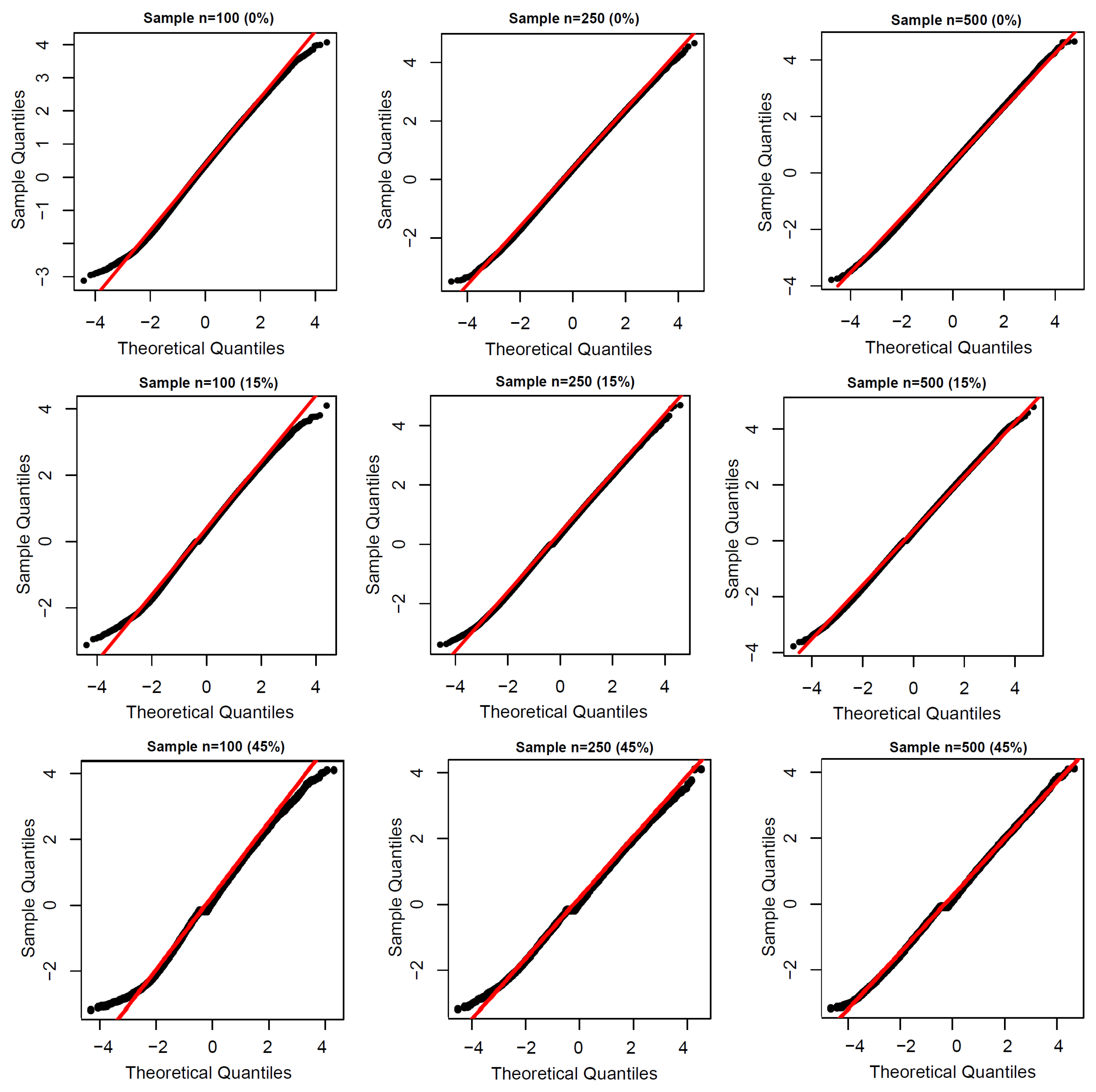
Figure 2 proves that the empirical distribution of the deviance residuals approximated the standard normal. So, the normal probability plot can be used with simulated envelopes.

5. Application to COVID-19 Data

We investigated the risk factors associated with death of diagnosed COVID-19 patients in the city of Campinas, Brazil. The sample was composed of hospitalized patients living in the city of Campinas or the northeastern area of the neighboring city of São Paulo in Brazil’s southeast region (Figure 3). A total of 322 patients infected with the virus (confirmed by RT-PCR screening) and classified as having Severe Acute Respiratory Syndrome 2 (SARS) were included in the study. The model was implemented in the gamlss script in the R software. The dataset and application codes can be accessed at https://github.com/gabrielamrodrigues/OLLW (accessed on 10 September 2022).
From an economic standpoint, Campinas has the eleventh largest municipal gross domestic product (GDP) in the country and was the first Brazilian city other than state capitals to be classified as a metropolis. It thus has significant national influence. In 2011, it was responsible for at least 15% of the nation’s scientific production and is the third-leading Brazilian city in terms of research and development. For these reasons and accuracy of the data, Campinas was selected in this study.
The response time t i (in days) is the period from the first symptoms until death due to COVID-19. In this sample, approximately 66.45% of the observations are censored, corresponding to patients who died for other reasons and patients who survived until the end of the study. The associated explanatory variables (for i = 1 , , 322 ) are: cens i : censoring indicator (0 = censored, 1 = time of life observed); x i 1 : sex (0 = female, 1 = male); x i 2 : age (in years); x i 3 : chronic cardiovascular disease (1 = yes, 0 = no or not informed); x i 4 : asthma (1 = yes, 0 = no or not informed); x i 5 : diabetes mellitus (1 = yes, 0 = no or not informed); x i 6 : chronic neurological disease (1 = yes, 0 = no or not informed); and x i 7 : obesity (1 = yes, 0 = no or not informed).

Descriptive Analysis

As in all statistical studies, we began with exploratory analysis of the data by studying the behavior of the response variable and its respective covariables. The Kaplan–Meier survival curves are presented in 
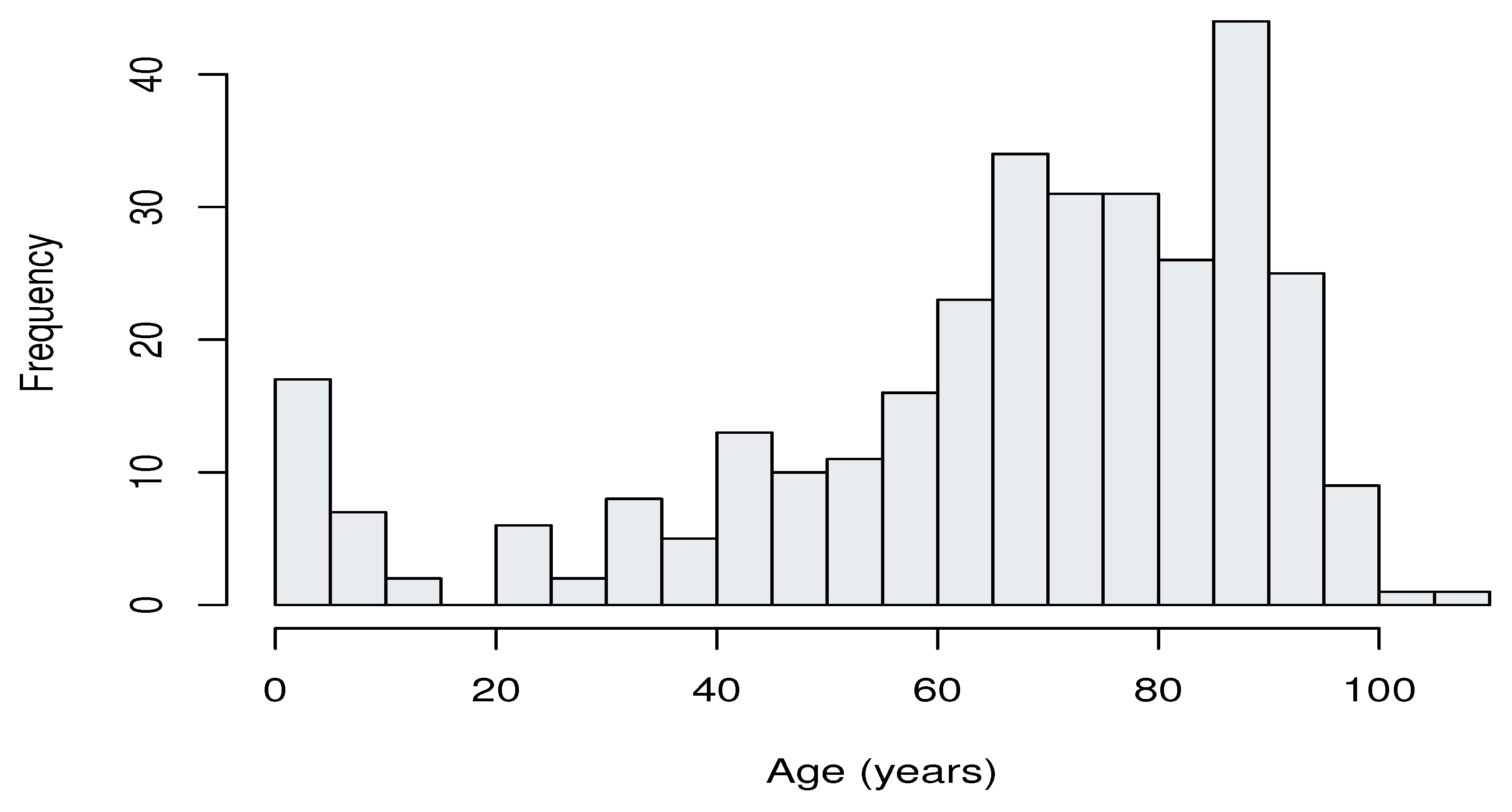
Figure 4, where it is possible to observe the existence of a higher risk of death among individuals suffering from diabetes or chronic neurological disease. In addition, Figure 5 clearly shows that patients aged from 65 to 90 years had the highest hospitalization frequency, as expected.
The MLEs and their standard errors (SEs) (in parentheses), as well as the Global Deviance (GD), Akaike Information Criterion (AIC), and Bayesian Information Criterion (BIC) from two fitted distributions to these data are given in Table 3.
The likelihood ratio (LR) statistic for comparing the OLLW and Weibull distributions ( w = 7.9 , p-value < 0.005 ) supports the first distribution. The estimated survival functions in Figure 6 also reveal this fact.
Further, the results from the fitted complete OLLW regression model
λ i = exp β 10 + j = 1 7 β 1 j x i j and α i = exp β 20 + j = 1 7 β 2 j x i j , i = 1 , , 322 ,
are reported in Table 4.
The variables age, asthma, diabetes mellitus, and chronic neurological disease are significant (at the level of 5%) for λ . For the parameter α , the age, asthma, diabetes, chronic neurological disease, and obesity variables are significant and hence the reduced OLLW regression model is
λ i = exp ( β 10 + β 12 x i 2 + β 15 x i 5 + β 16 x i 6 ) and α i = exp ( β 20 + β 22 x i 2 + β 26 x i 6 + β 27 x i 7 ) ,
whose estimation results are given in Table 5. Some interpretations on the numbers in this table are addressed at the end of this section.
The influence measures in Section 3.1 are calculated in R and displayed in Figure 7. They show that the 26th and 270th observations (referring to the patients below) are possibly influential:
  • 26th: A 64-year-old woman with comorbidities (cardiovascular disease, diabetes, and obesity) died in 6 days.
  • 270th: An 11-month-old baby with a neurological disease died in 5 days, and is the only patient younger than 1 year.
Figure 8a displays the index plot of the residuals ( r D i ) in Equation (11), thus revealing that they have a random behavior. Figure 8b reports the normal probability plot with a simulated envelope (Atkinson, 1987 [25]), thus revealing that the reduced OLLW regression model is appropriate for these data.
The plots of the empirical and estimated survival functions for the two categorical variables in Figure 9 confirm the adequacy of the fitted regression.
Interpretation for λ
  • The survival time declines when the age increases.
  • Diabetes mellitus has a significant effect in reducing the survival time of COVID-19 patients.
  • The patients with chronic neurological disease have a significant reduction in survival time.
Interpretation for α
  • The patient age is also significant in terms of survival time variability.
  • The variability of survival time depends on whether the patient is obese or not.
  • The variability of survival time depends on whether the patient has chronic neurological disease or not.
Finally, we obtain S ( t | x i ) from Equation (9). In Figure 10, the estimated survival and hazard rates are plotted for the four hypothetical patients described earlier. Figure 10a reveals that patients with diabetes mellitus and chronic neurological diseases have a shorter survival time than those who do not have these diseases. Similarly, Figure 10b shows that patients with diabetes and chronic neurological diseases are at higher risk compared to patients who do not have these pathologies.
We can obtain the survival probabilities and median times from Equations (9) and (4), respectively. Then, we consider x 7 fixed at 0 and x 2 and x 6 , as shown in Table 6. Table 7 and Table 8 show the probability of hospitalized patients surviving 20 days after the first symptom and the median time for some ages, respectively.

6. Conclusions

This work studied the factors that increase the risk of death of hospitalized patients diagnosed with COVID-19 using the odd log-logistic Weibull regression model with two systematic components. Some new general structural properties of this model were provided such as its stochastic representation, identifiability, and moments, among others. A simulation study was carried out to evaluate the proposed regression model, which revealed the consistency of the maximum likelihood estimators and showed that the empirical coverage probabilities were close to the nominal level and that the empirical distribution of the deviance modified residuals approached the standard normal.
The application to COVID-19 data revealed some important results. The older age group was a predictor of a higher death rate from COVID-19, corroborating studies by Giacomelli et al. (2020) [12] and Atlam et al. (2021) [14], and diabetes and obesity were also evidenced in this work as determinants for the survival of infected patients, as discussed in Giacomelli et al. (2020) [12], Albitar et al. (2020) [16], and Noor et al. (2020) [17]. Chronic neurological diseases were also identified as risk factors, but we emphasize that few studies have obtained these results (García-Azorín et al. (2020) [18] and Noor et al. (2020) [17]). Therefore, it is recommended to consider the presence of this comorbidity in future studies in the assessment of mortality risk, as well as verify its significance in other datasets. Several studies have also indicated that men are at greater risk of death (see Albitar et al. (2020) [16] and Liu et al. (2020) [19]). However, no significant differences were found between the sexes. Chronic cardiovascular disease and asthma also did not prove to be determinants for the survival of individuals in this study.
It is suggested that future works verify the current datasets and those from other cities, as well as verify whether the same covariates would be significant in a lifetime analysis.
It is possible to conclude that the proposed regression proved to be efficient in identifying the factors that influenced the survival of individuals in this dataset, which can help more timely and efficient medical interventions. Finally, this model can be considered an interesting alternative for future works that evaluate censored lifetimes.

Author Contributions

Conceptualization, G.M.R., E.M.M.O., G.M.C. and R.V.; methodology, G.M.R., E.M.M.O., G.M.C. and R.V.; software, G.M.R., E.M.M.O., G.M.C. and R.V.; validation, G.M.R., E.M.M.O., G.M.C. and R.V.; formal analysis, G.M.R., E.M.M.O., G.M.C. and R.V.; investigation, G.M.R., E.M.M.O., G.M.C. and R.V.; data curation, G.M.R., E.M.M.O., G.M.C. and R.V.; writing—original draft preparation, G.M.R., E.M.M.O., G.M.C. and R.V.; writing—review and editing, G.M.R., E.M.M.O., G.M.C. and R.V.; visualization, G.M.R., E.M.M.O., G.M.C. and R.V.; supervision, G.M.R., E.M.M.O., G.M.C. and R.V. All authors have read and agreed to the current version of the manuscript.

Funding

This study was financed in part by the Coordenação de Aperfeiçoamento de Pessoal de Nível Superior-Brasil (CAPES) (Finance Code 001).

Institutional Review Board Statement

Not applicable.

Informed Consent Statement

Not applicable.

Data Availability Statement

The authors confirm that the data supporting the findings of this study are available within the article.

Conflicts of Interest

The authors declare no conflict of interest.

References

  1. Da Cruz, J.N.; Ortega, E.M.M.; Cordeiro, G.M. The log-odd log-logistic Weibull regression model: Modelling, estimation, influence diagnostics and residual analysis. J. Stat. Comput. Simul. 2016, 86, 1516–1538. [Google Scholar] [CrossRef]
  2. Da Cruz, J.N.; Ortega, E.M.M.; Cordeiro, G.M.; Suzuki, A.K.; Mialhe, F.L. Bivariate odd-log-logistic-Weibull regression model for oral health-related quality of life. Commun. Stat. Appl. Methods 2017, 24, 271–290. [Google Scholar] [CrossRef] [Green Version]
  3. De Freitas Costa, E.; Schneider, S.; Carlotto, G.B.; Cabalheiro, T.; de Oliveira, M.R., Jr. Zero-inflated-censored Weibull and gamma regression models to estimate wild boar population dispersal distance. Jpn. J. Stat. Data Sci. 2021, 4, 1133–1155. [Google Scholar] [CrossRef]
  4. Al-Dawsari, S.R.; Sultan, K.S. Inverted Weibull Regression Models and Their Applications. Stats 2021, 4, 269–290. [Google Scholar] [CrossRef]
  5. Sánchez, L.; Leiva, V.; Saulo, H.; Marchant, C.; Sarabia, J.M. A new quantile regression model and its diagnostic analytics for a Weibull distributed response with applications. Mathematics 2021, 9, 2768. [Google Scholar] [CrossRef]
  6. Moamer, S.; Baghestani, A.; Pourhoseingholi, M.A.; Hajizadeh, N.; Ahmadi, F.; Norouzinia, M. Evaluation of prognostic factors effect on survival time in patients with colorectal cancer, based on Weibull Competing-Risks Model. Gastroenterol. Hepatol. Bed Bench 2017, 10, 54–59. [Google Scholar]
  7. Yoosefi, M.; Baghestani, A.R.; Khadembashi, N.; Pourhoseingholi, M.A.; Baghban, A.A.; Khosrovirad, A. Survival analysis of colorectal cancer patients using exponentiated Weibull distribution. Int. J. Cancer Manag. 2018, 11, e8686. [Google Scholar] [CrossRef]
  8. Naseri, P.; Baghestani, A.R.; Momenyan, N.; Akbari, M.E. Application of a mixture cure fraction model based on the generalized modified weibull distribution for analyzing survival of patients with breast cancer. Int. J. Cancer Manag. 2018, 11, e62863. [Google Scholar] [CrossRef]
  9. Pavisic, I.M.; Nicholas, J.M.; O’Connor, A.; Rice, H.; Lu, K.; Fox, N.C.; Ryan, N.S. Disease duration in autosomal dominant familial Alzheimer disease: A survival analysis. Neurol. Genet. 2020, 6, e507. [Google Scholar] [CrossRef]
  10. Xavier, D.R.; Morais, I.; Magalhães, M.; Saldanha, R.; Dantas, R.; Barcellos, C.; Stenner, C. Nota Técnica 24 de 10 de Fevereiro de 2022. O avanço da Variante Ômicron, a Resposta das Vacinas e o Risco de Desassistência. 2022. Available online: https://www.arca.fiocruz.br/handle/icict/51252 (accessed on 10 September 2022).
  11. Lu, W.; Yu, S.; Liu, H.; Suo, L.; Tang, K.; Hu, J.; Hu, K. Survival analysis and risk factors in COVID-19 patients. In Disaster Medicine and Public Health Preparedness; Cambridge University Press: Cambridge, UK, 2021; pp. 1–6. [Google Scholar] [CrossRef]
  12. Giacomelli, A.; Ridolfo, A.L.; Milazzo, L.; Oreni, L.; Bernacchia, D.; Siano, M.; Bonazzetti, C.; Covizzi, A.; Schiuma, M.; Passerini, M.; et al. 30-day mortality in patients hospitalized with COVID-19 during the first wave of the Italian epidemic: A prospective cohort study. Pharmacol. Res. 2020, 158, 104931. [Google Scholar] [CrossRef] [PubMed]
  13. Zheng, Z.; Peng, F.; Xu, B.; Zhao, J.; Liu, H.; Peng, J.; Li, Q.; Jiang, C.; Zhou, Y.; Liu, S.; et al. Risk factors of critical and mortal COVID-19 cases: A systematic literature review and meta-analysis. J. Infect. 2020, 81, 16–25. [Google Scholar] [CrossRef]
  14. Atlam, M.; Torkey, H.; El-Fishawy, N.; Salem, H. Coronavirus disease 2019 (COVID-19): Survival analysis using deep learning and Cox regression model. Pattern Anal. Appl. 2021, 24, 993–1005. [Google Scholar] [CrossRef]
  15. Nijman, G.; Wientjes, M.; Ramjith, J.; Janssen, N.; Hoogerwerf, J.; Abbink, E.; van de Maat, J.S. Risk factors for in-hospital mortality in laboratory-confirmed COVID-19 patients in The Netherlands: A competing risk survival analysis. PLoS ONE 2021, 16, e0249231. [Google Scholar] [CrossRef]
  16. Albitar, O.; Ballouze, R.; Ooi, J.P.; Ghadzi, S.M.S. Risk factors for mortality among COVID-19 patients. Diabetes Res. Clin. Pract. 2020, 166, 108293. [Google Scholar] [CrossRef] [PubMed]
  17. Noor, F.M.; Islam, M. Prevalence and associated risk factors of mortality among COVID-19 patients: A meta-analysis. J. Commun. Health 2020, 45, 1270–1282. [Google Scholar] [CrossRef] [PubMed]
  18. García-Azorín, D.; Martínez-Pías, E.; Trigo, J.; Hernández-Pérez, I.; Valle-Peñacoba, G.; Talavera, B.; Simón-Campo, P.; de Lera, M.; Chavarría-Mir, A.; López-Sanz, C.; et al. Neurological comorbidity is a predictor of death in Covid-19 disease: A cohort study on 576 patients. Front. Neurol. 2020, 11, 781. [Google Scholar] [CrossRef] [PubMed]
  19. Liu, Y.; Du, X.; Chen, J.; Jin, Y.; Peng, L.; Wang, H.H.; Zhao, Y. Neutrophil-to-lymphocyte ratio as an independent risk factor for mortality in hospitalized patients with COVID-19. J. Infect. 2020, 81, 6–12. [Google Scholar] [CrossRef]
  20. Yang, J.; Zheng, Y.A.; Gou, X.; Pu, K.; Chen, Z.; Guo, Q.; Ji, R.; Wang, H.; Wang, Y.; Zhou, Y. Prevalence of comorbidities and its effects in patients infected with SARS-CoV-2: A systematic review and meta-analysis. Int. J. Infect. Dis. 2020, 94, 91–95. [Google Scholar] [CrossRef]
  21. Gleaton, J.U.; Lynch, J.D. Properties of generalized log-logistic families of lifetime distributions. J. Probab. Stat. Sci. 2006, 4, 51–64. [Google Scholar]
  22. Cook, R.D. Assesment of local influence (with discussion). J. R. Stat. Soc. 1986, 48, 133–169. [Google Scholar]
  23. Cook, R.D.; Peña, D.; Weisberg, S. The likelihood displacement: A unifying principle for influence measures. Commun. Stat. Theor. Methods 1988, 17, 623–640. [Google Scholar] [CrossRef]
  24. Escobar, L.A.; Meeker, W.Q. Assessing influence in regression analysis with censored data. Biometrics 1992, 48, 507–528. [Google Scholar] [CrossRef] [PubMed]
  25. Atkinson, A.C. Plots, Transformations and Regression: An Introduction to Graphical Methods of Diagnostics Regression Analysis, 2nd ed.; Clarendon Press: Oxford, UK, 1987. [Google Scholar]
Figure 1. Plots of the OLLW density. (a) Changing τ , λ = 1.5 and α = 5 . (b) Changing λ , α = 5 and τ = 0.3 .
Mathematics 10 03644 g001
Figure 2. Normal probability plots of r D i ’s for n = 100 , 250, and 500, and censoring percentages 0 % , 10 % , and 30 % .
Mathematics 10 03644 g002
Figure 3. Location of the city of Campinas, São Paulo, Brazil.
Mathematics 10 03644 g003
Figure 4. Kaplan–Meier survival curves: (a) Sex; (b) Chronic cardiovascular disease; (c) Diabetes mellitus; (d) Obesity; (e) Asthma and (f) Chronic neurological disease.
Mathematics 10 03644 g004
Figure 5. Histogram of the covariate “age”.
Mathematics 10 03644 g005
Figure 6. The estimated and empirical survival functions for COVID-19 data.
Mathematics 10 03644 g006
Figure 7. Index plots for (a) G D i ( θ ) and (b) L D i ( θ ) .
Mathematics 10 03644 g007
Figure 8. (a) Index plot of r D i . (b) Normal probability plot for r D i with envelope.
Mathematics 10 03644 g008
Figure 9. Estimated and empirical survival functions: (a) Diabetes mellitus; (b) chronic neurological disease.
Mathematics 10 03644 g009
Figure 10. (a) Estimated survival functions. (b) Estimated hazard functions.
Mathematics 10 03644 g010
Table 1. Findings for the averages, biases, and MSEs from the simulated OLLW regression model.
n = 100 n = 250 n = 500
% θ AveragesBiasesMSEsAveragesBiasesMSEsAveragesBiasesMSEs
0 % β 10 3.00220.00220.00023.00120.00120.00013.00050.00050.0000
β 11 2.4989−0.00110.00012.4999−0.00010.00012.50010.00010.0000
β 12 0.8997−0.00030.00010.8999−0.00010.00000.90020.00020.0000
β 20 2.03590.03590.13922.00650.00650.04852.00380.00380.0205
β 21 1.50780.00780.09001.4925−0.00750.03251.50300.00300.0145
β 22 0.7987−0.00130.02700.7948−0.00520.01140.7996−0.00040.0049
β 30 0.2832−0.01680.12300.30850.00850.04360.2999−0.00010.0182
15 % β 10 3.00130.00130.00023.00160.00160.00013.00090.00090.0000
β 11 2.4992−0.00080.00022.4993−0.00070.00012.4998−0.00020.0000
β 12 0.90030.00030.00010.8999−0.00010.00000.90010.00010.0000
β 20 2.08070.08070.16052.00520.00520.05452.00200.00200.0260
β 21 1.50200.00200.10301.4899−0.01010.03631.50120.00120.0179
β 22 0.7880−0.01200.03440.7899−0.01010.01230.7964−0.00360.0066
β 30 0.2459−0.05410.13690.31290.01290.04870.30510.00510.0240
45 % β 10 3.00120.00120.00033.00190.00190.00013.00140.00140.0001
β 11 2.4990−0.00100.00032.4989−0.00110.00012.4994−0.00060.0000
β 12 0.90020.00020.00010.90010.00010.00000.9000−0.00000.0000
β 20 2.14520.14520.20342.02720.02720.08742.02320.02320.0402
β 21 1.4288−0.07120.15591.4671−0.03290.05371.4798−0.02020.0287
β 22 0.7598−0.04020.05350.7766−0.02340.01780.7863−0.01370.0092
β 30 0.2299−0.07010.15030.31100.01100.07750.2950−0.00500.0391
Table 2. CPs for the 95% confidence intervals from the simulated OLLW regression model.
0 % 10 % 30 %
n 100250500100250500100250500
β 10 0.9570.9620.9700.9590.9570.9660.9650.9620.967
β 11 0.9520.9600.9660.9570.9600.9710.9370.9610.966
β 12 0.9560.9680.9550.9440.9620.9610.9500.9580.962
β 20 0.9230.9490.9640.9030.9620.9580.9250.9470.943
β 21 0.9470.9530.9590.9480.9520.9480.9690.9640.958
β 22 0.9460.9330.9570.9450.9520.9320.9460.9620.949
β 30 0.9380.9600.9680.9240.9670.9690.9580.9680.952
Table 3. Estimation results.
Model λ α τ GDAICBIC
OLLW20.67505.65230.3113916.9922.9934.2
(0.9375)(1.4702)(0.0880)
Weibull22.57111.75101924.8928.8936.3
(1.4116)(0.1326)
Table 4. Findings from the complete OLLW regression.
MLEsSEsp-Values MLEsSEsp-Values
β 10 4.30210.0754<0.0001 β 20 1.70130.0410<0.0001
β 11 −0.09740.06800.1531 β 21 0.08420.05530.1288
β 12 −0.01590.0012<0.0001 β 22 −0.00550.0010<0.0001
β 13 0.07720.08410.3596 β 23 0.13070.09460.1679
β 14 −0.41900.13350.0019 β 24 0.36030.11340.0016
β 15 −0.24430.08810.0059 β 25 −0.28960.11600.0131
β 16 −0.35460.14680.0163 β 26 −0.38800.16770.0213
β 17 −0.02770.11470.8094 β 27 0.50950.19040.0078
log ( τ ) −0.69330.0263
AIC: 895.7497; BIC: 959.9171; GD: 861.7497
Table 5. Findings from the reduced OLLW regression model.
MLEsSEsp-Values
β 10 4.08610.0644<0.0001
β 12 −0.01300.0012<0.0001
β 15 −0.26960.08180.0011
β 16 −0.32110.16250.0490
β 20 1.43040.0364<0.0001
β 22 −0.00630.0009<0.0001
β 26 −0.36220.17080.0347
β 27 0.50110.20230.0138
log ( τ ) −0.33370.0269
AIC: 884.7161; BIC: 918.6871; GD: 866.7161
Table 6. Four selected patients.
PatientAgeDiabetes MellitusChronic Neurological Disease
A50YesYes
B50YesNo
C50NoYes
D50NoNo
Table 7. Probability of hospitalized patients surviving 20 days after the first symptom.
Age306090
Patient A0.470.250.11
Patient B0.730.430.17
Patient C0.620.400.22
Patient D0.850.620.35
Table 8. Median time for some ages.
Age306090
Patient A19.1512.558.17
Patient B27.6518.3012.05
Patient C25.0816.4310.70
Patient D36.2123.9615.78
Publisher’s Note: MDPI stays neutral with regard to jurisdictional claims in published maps and institutional affiliations.

