A Modified Inverse Iteration Method for Computing the Symmetric Tridiagonal Eigenvectors

Abstract

This paper presents a novel method for computing the symmetric tridiagonal eigenvectors, which is the modification of the widely used Inverse Iteration method. We construct the corresponding algorithm by a new one-step iteration method, a new reorthogonalization method with the general Q iteration and a significant modification when calculating severely clustered eigenvectors. The numerical results show that this method is competitive with other existing methods, especially when computing part eigenvectors or severely clustered ones.

1. Introduction

Computing the symmetric tridiagonal (ST) eigenvector is an important task in many research fields, such as the computational quantum physics [1], mathematics [2,3], dynamics [4], computational quantum chemistry [5], etc. The ST eigenvector problem also arises while solving any symmetric eigenproblem because it is a common practice to reduce the generalized symmetric eigenproblems to an ST one.

The Divide and Conquer (DC) algorithm [6] has a considerable advantage when calculating all the eigenpairs of an ST matrix. It is quite remarkable that the DC method, which is efficient for parallel computation, can also be faster than other implementations on a serial computer. However, this method does not support computing part eigenpairs or computing eigenvectors only. In practice, it is rare to compute the full eigenvectors of a large ST matrix. The famous QR method [7] has the same shortage while costing more time and is hard to be parallelized. This paper focuses on modifying the solution of computing part eigenvectors and gives a new method for eigenvectors of good accuracy and orthogonality.

Once an accurate eigenvalue approximation is known, the Inverse Iteration method [8] always computes an accurate eigenvector with an acceptable time cost. However, it does not guarantee the orthogonality when eigenvalues are close. A commonly used remedy is to reorthogonalize each approximate eigenvector, by the modified Gram–Schmidt method, against previously computed eigenvectors in the cluster. This remedy increases up to $2n^3$ operations if all the eigenvalues cluster, while the time cost for the eigenvectors themselves is only $O\left(n^2\right)$.

Dhillion proposed the Multiple Relatively Robust Representations (MRRR) algorithm [9] to avoid reorthogonalization. This is an ambitious attempt as the MRRR algorithm computes all the accurate and numerically orthogonal eigenvectors with a time cost of $O\left(n^2\right)$. Nevertheless, the MRRR algorithm can fail in calculating severely clustered eigenvalues of a large group, such as the glued Wilkinson matrices [10]. Dhillion fixed the problem and modified the MRRR method subtly and cleverly [11], without increasing its time complexity. However, this modified MRRR method, which applies the perturbation to the root representation of the ST matrix, costs even more time than the Inverse Iteration method with the modified Gram–Schmidt process. Even when computing random matrices, the MRRR algorithm has no advantage compared with the Inverse Iteration method. In addition, when computing part eigenvectors, the MRRR algorithm needs considerably accurate eigenvalues to guarantee natural orthogonality and thus calls the time-consuming Bisection method to obtain them. As a consequence, except for those cases with many eigenvalues clusters, the Inverse Iteration method is more efficient. More related details are presented in Section 6.

Mastronardi and Van Dooreen [12] proposed an ingenious method to determine the accurate eigenvector of a symmetric tridiagonal matrix once an approximation of the eigenvalue is known. In addition, they applied this method to calculate the weights of the Gaussian quadrature rules [3].

Our strategy is to improve the Inverse Iteration method with the three main modifications:

• We replace the iteration process with a new one that only costs one step to guarantee convergence, similar to the MRRR method;
• The envelope vector theory [13] is utilized to compute accurate and naturally orthogonal eigenvectors when the eigenvalues severely cluster. By combining the new iteration process, the time cost is even less than the cost of calculating isolated eigenvectors. In other words, the severely clustered eigenvalues accelerate the convergence;
• We give a new orthogonalization method for the generally clustered groups of severely clustered eigenvalues. For k clustered eigenvalues in such a case, the new orthogonalization method decreases the time cost from $O\left(n{k}^2\right)$ to $O\left(nk\right)$.

The numerical results confirm our promise of accuracy and orthogonality. In addition, our new method supports computing part eigenvectors and embarrassingly parallelization, significantly improving the computational efficiency.

This paper focuses on the symmetric tridiagonal eigenvector problem. According to Weyl’s theorem, the real symmetric eigenvalue problem $Ax=x\lambda$ is well posed, in an absolute sense because an eigenvalue can change by no more than the spectral norm of the change in the matrix A [14]. However, for an unsymmetric matrix $\widehat{A}$, some of its eigenvalues may be extremely sensitive to uncertainty in the matrix entries. Consequently, the assessment of error becomes a major concern. Some specific conclusions were introduced in [14]. Readers can also see more unsymmetric examples in [15,16].

The organization of the rest of this paper is as follows: Section 2 gives the modified iteration of the new method and an algorithm to compute an isolated eigenvector. Section 3 studies the computation of clustered eigenvectors. Section 4 introduces the general Q iteration and the new orthogonalization method. Section 5 concerns the overflow and underflow. Several corresponding pseudocodes are provided in the above sections. Section 6 shows some examples and numerical results. Finally, we discuss and assess the Modified Inverse Iteration method in Section 7.

2. Compute Isolated Eigenvectors

2.1. Theoretical Background

Consider a $n\times n$ real unreduced ST matrix A (all the ST matrices discussed in this paper are real and unreduced), which has eigenvalues ${\lambda }_1\sim {\lambda }_n$ in the increasing order and the corresponding eigenvectors $v_1\sim v_n$. Once an accurate eigenvalue approximation $u\to {\lambda }_j$ is known, we have

$$(A-u{I}_{n\times n})\widetilde{v_j}=T\widetilde{v_j}=0,$$

(1)

where $\widetilde{v_j}$ is the eigenvector approximation and $I_{n\times n}$ denotes the $n\times n$ identity matrix.

When u is the exact eigenvalue, T has a rank of $n-1$ and (1) can be solved by ignoring any one of its n rows. However, since $u\ne {\lambda }_j$, T is not singular and thus (1) has no nonzero solution. If one still solves (1) by ignoring one of its n rows, say, the kth row, the actually solved equation is

$$T{z}^k=e_k,$$

(2)

where $e_k$ is the kth column of $I_{n\times n}$, and $z^k$ denotes the solution when ignoring the k row. It is obvious that $z^k$ is the kth column of $T^{-1}$. From [10], we have

$$z^k=r_j{v}_j/\left({\lambda }_j-u\right)+\sum _{i\ne j}{r}_i{v}_i/\left({\lambda }_i-u\right),$$

(3)

where $r_i(i\in [1,n])$ is the kth component of $v_i$, which can also be denoted by $v_i\left(k\right)$.

The main idea of the Inverse Iteration is to solve (2), substitute the result into the right side, and go on. As $u\to {\lambda }_j$, $z^k$ will finally approach $v_j$. If ${\lambda }_j$ is an isolated eigenvalue, (3) shows that the degree of approximation of $z^k$ and $v_j$ depends on the absolute value of $v_j\left(k\right)$. For example, if $|v_j\left(k\right)|$ approximates to zero, $z^k$ has nearly no ingredient of $v_j$. As a consequence, the iterations hardly converge. Therefore, the traditional Inverse Iteration method uses a vector with all components equal to 1 to be the original right side of (1). Within about two or three steps, the traditional Inverse Iteration method calculates an accurate eigenvector approximation $\widetilde{v_j}$.

2.2. One-Step Iteration

To accelerate the iteration process, our task is to find the biggest $|v_j\left(k\right)|(k\in [1,n])$ and to guarantee convergence in one step. From [9], we have

$$\frac{1}{{\gamma }_k}=e_k^T{(A-uI)}^{-1}{e}_k=\frac{{\left|v_j\left(k\right)\right|}^2}{{\lambda }_j-u}+\sum _{i\ne j}\frac{{\left|v_i\left(k\right)\right|}^2}{{\lambda }_i-u}$$

(4)

where $1/{\gamma }_k$ is the kth component on the diagonal of ${(A-uI)}^{-1}$, i.e., the kth component of $z^k$, and its absolute value reflects $|v_j\left(k\right)|$ (recall $u\to {\lambda }_j$). The MRRR method finds the smallest $|{\gamma }_k|$ by the twisted triangular factorization, while we give a new method in this section.

We denote the ith sequential principal minor of a ST matrix A by $A_{1:i}$. The submatrix of A in rows i through j is denoted by $A_{i:j}$ and its determinant by $det\left(A\right)$. We denote the characteristic polynomial $det(A-uI)$ by $C_{1:n}$, $C_{1:n}\left(u\right)$, or $C_{1:n}^A\left(u\right)$ if necessary. $a_i$ and $b_i$ denote the ith component on the diagonal and sub-diagonal of A, respectively. According to [17], we have

$$z^k=\left[\begin{array}{c}{C}_{k+1:n}\left({\displaystyle \prod _{t=1}^{k-1}}-b_t\right)\\ C_1{C}_{k+1:n}\left({\displaystyle \prod _{t=2}^{k-1}}-b_t\right)\\ \dots \\ C_{1:k-2}{C}_{k+1:n}(-b_{k-1})\\ C_{1:k-1}{C}_{k+1:n}\\ C_{1:k-1}{C}_{k+2:n}(-b_k)\\ \dots \\ C_{1:k-1}{C}_n\left({\displaystyle \prod _{t=k}^{n-2}}-b_t\right)\\ C_{1:k-1}\left({\displaystyle \prod _{t=k}^{n-1}}-b_t\right)\end{array}\right]/C_{1:n}$$

(5)

and

$$\begin{array}{cc}\hfill C_{1:n}& =det(A-uI)\hfill \\ \hfill & =-b_{k-1}^2{C}_{1:k-2}{C}_{k+1:n}+(a_k-u)C_{1:k-1}{C}_{k+1:n}-b_k^2{C}_{1:k-1}{C}_{k+2:n}\hfill \\ \hfill & =C_{1:k-1}{C}_{k+1:n}(C_{1:k}/C_{1:k-1}-b_k^2{C}_{k+2:n}/C_{k+1:n}).\hfill \end{array}$$

(6)

Remark 1.

(5) is also introduced in [9], but in an incorrect form as missing the negative sign before each $b_i$. Dhillion worried about the overflow and underflow issues when calculating $z^k$ by (5) and thus did not discuss it further. This paper will give a more practical form of (5), reduce its computational cost and solve the overflow or underflow problem (in Section 5).

By (5) and (6), we have

$${\gamma }_k=q_k-b_k^2/p_{n-k}$$

(7)

where $q_i=C_i/C_{i-1}$ and $p_i=C_{n-i+1}/C_{n-i+2}$. As the sequential principal minors of an ST matrix form a Sturm sequence, we have [18]

$$\begin{array}{c}{q}_0=1,q_1=a_1-u,q_i=a_i-u-b_{i-1}^2/q_{i-1};\\ p_0=1,p_1=a_n-u,p_i=a_{n+1-i}-u-b_{n+1-i}^2/p_{i-1}.\end{array}$$

(8)

(5) and (8) can be expressed as

$$z^k=x_1\alpha +x_2\beta =\left[\begin{array}{c}1\\ q_1/(-b_1)\\ q_1{q}_2/\left((-b_1)(-b_2)\right)\\ \dots \\ {\displaystyle \prod _{i=1}^{k-1}}{q}_i/(-b_i)\\ 0\\ \dots \\ 0\\ 0\end{array}\right]\alpha +\left[\begin{array}{c}0\\ 0\\ \dots \\ 0\\ {\displaystyle \prod _{i=1}^{n-k-1}}{p}_i/(-b_{n-i})\\ \dots \\ p_1{p}_2/\left((-b_{n-1})(-b_{n-2})\right)\\ p_1/(-b_{n-1})\\ 1\end{array}\right]\beta ,$$

(9)

where $x_1$ and $x_2$ are both $n\times 1$ vectors, the $(k+1)\sim n$th components of $x_1$ are zeros while the $1\sim k$th components of $x_2$ are zeros. $\alpha$ and $\beta$ are two coefficients to be determined.

It can be seen that (9) satisfies (2), except for the kth and $(k+1)$th rows. As we only care about the direction of $z^k$, only the $(k+1)$th row needs to be considered when determining $\alpha$ and $\beta$. Then, we have

$$\alpha b_k\prod _{i=1}^{k-1}{q}_i/(-b_i)+\beta \left((a_{k+1}-u)\left(\prod _{i=1}^{n-k-1}{p}_i/(-b_{n-i})\right)+b_{k+1}\left(\prod _{i=1}^{n-k-2}{p}_i/(-b_{n-i})\right)\right)=0.$$

Therefore, our scheme is to calculate $q_i$’s and $p_i$’s by (8) first, then find the smallest $|{\gamma }_k|$ by (7). Note that (7) would not cost extra division operations if we save the $b_i^2/p_{n-i}$’s when calculating $p_i$’s by (8). Finally, we choose the corresponding k of the smallest $|{\gamma }_k|$ and obtain $z^k$ by (9). Our modified iteration method to calculate one isolated eigenvector is shown by Algorithm 1.

If $b_i^2$ and $1/b_i$ are calculated and stored in advance, Algorithm 1 costs $8n\sim 8.5n$ operations (note the cost of calculating $a-u$ is shared in step 3 of Algorithm 1) per eigenvector while the version in [9] costs $11n$.

Note that (8) computes p and q with no time cost savings per se. The two main contributors are: first, (7) reduces the cost of searching $min|{\gamma }_k|$; second, (9) divides the eigenvector computation into two parts, and even under the most adverse condition of $k=n/2$, (9) can still reduce the multiplication operations by half compared to (5).

Algorithm 1: Compute one isolated eigenvector.

2.3. Accuracy Analysis of Algorithm 1

Let R denote the residual norm, i.e., $R_k=∥T{z}^k∥/∥z^k∥$, then we have

$$\begin{array}{cc}\hfill R_k& =\frac{∥T{z}^k∥}{∥z^k∥}=\frac{\left|{\gamma }_k\right|}{∥z^k∥}\hfill \\ \hfill & =\sqrt{\frac{{\gamma }_k^2}{{\gamma }_k^2{e}_k^T{\left(A-uI\right)}^{-1}{\left(A-uI\right)}^{-1}{e}_k}}\hfill \\ \hfill & ={\left(\sum _{}\frac{v_i^2\left(k\right)}{{\left({\lambda }_i-u\right)}^2}\right)}^{-1/2}=\frac{\left|{\lambda }_j-u\right|}{\left|v_j\left(k\right)\right|}{\left(1+\sum _{}\frac{{\left({\lambda }_j-u\right)}^2}{{\left({\lambda }_i-u\right)}^2}\frac{v_i^2\left(k\right)}{v_j^2\left(k\right)}\right)}^{-1/2}\hfill \\ \hfill & \le \frac{\left|{\lambda }_j-u\right|}{\left|v_j\left(k\right)\right|}.\hfill \end{array}$$

(10)

As Algorithm 1 ensures that $|v_j\left(k\right)|$ is the biggest one among all the $|v_j\left(i\right)|(i\in [1,n])$, it is guaranteed that $|v_j\left(k\right)|\ge \sqrt{1/n}$. Then, according to (10), we have $R_k\le \sqrt{n}ϵ$ where $ϵ$ is the machine precision.

3. Computing Severely Clustered Eigenvectors

Now consider the case when eigenvalues clusters severely, for example, p eigenvalues that are equal in finite precision arithmetic. We will define “severely clustering” later in this section.

First, we introduce the two following lemmas from [13] to state our theorems.

Lemma 1

(The Envelope Vector). Define $\mathcal{S}=span\{v_1,v_2,\dots ,v_p\}$, and the envelope vector of $\mathcal{S}$ is $\mathcal{E}$ given by

$${\mathcal{E}}_i=max\{{\mathcal{V}}_i:\mathcal{V}\in \mathcal{S},∥\mathcal{V}∥=1\}.$$

For p clustered eigenvalues, the envelope vector will undulate with p high hills separated by $p-1$ low valleys.

Lemma 2.

For an ST matrix A that has p clustered eigenvalues ${\lambda }_1\sim {\lambda }_p$, divide A into p submatrices: $A_{1:{\eta }_1}$, $A_{{\eta }_2^l:{\eta }_2^r}$,…, $A_{{\eta }_{p-1}^l:{\eta }_{p-1}^r}$ and $A_{{\eta }_p:n}$. Note that these submatrices can have overlaps. Then, for each submatrix, there exists at least one $A_{sub}$, among all the possibilities of divisions that satisfies:

1 

$A_{sub}$ has an isolated sub-eigenvalue $\kappa \in [{\lambda }_1,{\lambda }_p]$;

2 

For the 2nd to $(p-1)$th submatrices, the corresponding sub-eigenvector $s_i(i\in [2,p-1])$ (with respect to κ) has small components at both its ends. For $A_{1:{\eta }_1}$, $s_1\left({\eta }_1\right)\to 0$ and for $A_{{\eta }_p:n}$, $s_p\left(1\right)\to 0$.

Supplement zero components to obtain ${\tilde{v}}_s=[s;0]$, $[0;s;0]$, or $[0;s]$, which has the size of $n\times 1$. Then, the p ${\tilde{v}}_s$’s are approximations to $v_t(t\in [1,p])$. These eigenvector approximations are numerical orthogonal and satisfy $∥T{v}_s∥<\sqrt{n/p}({\lambda }_p-{\lambda }_1)/p$.

See the proofs and more details in [13].

Let us take a typical example of clustered eigenvalues to illustrate. Let ${\alpha }_0$ be a $200\times 1$ vector and ${\alpha }_0\left(i\right)=i(i\in [1,200])$ and then construct $\alpha \leftarrow [flip\left({\alpha }_0\right);0;{\alpha }_0]$. Then, repeat $\alpha \leftarrow [\alpha ;{\alpha }_0]$ by eight times totally. Finally, we obtain a $2001\times 1$ vector $\alpha$. Consider an ST matrix $\Phi$, which has the diagonal equal to $\alpha$ and all the components on its sub-diagonal equal to 1. $\Phi$ is similar to the glued Wilkinson matrices in [11] and its biggest eight eigenvalues (${\lambda }_1\sim {\lambda }_8$) cluster severely. Let $u_1\sim u_8$ denote the approximations of the biggest eight eigenvalues of $\Phi$; it shows $u_8-u_1=0$ in Matlab, i.e., ${\lambda }_1\sim {\lambda }_8$ severely clusters.

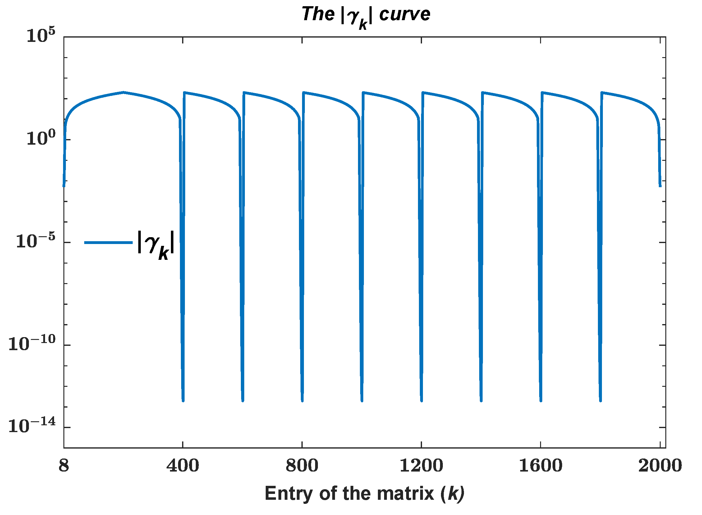
Let $u=u_1$ and calculate $|{\gamma }_k|(k\in [1,2001])$ of $\Phi$. The results are shown in Figure 1. According to Lemma 1, the low valley entries of the envelope vector correspond to small components of $v_i(i\in [1,p])$. Note that this means all the p eigenvectors have small components at this entry, thus the corresponding $|{\gamma }_k|$ must be a big value according to (4). The case of high hills is similar. In other words, the $|{\gamma }_k|$ curve undulates with p low valleys separated by $p-1$ high hills. Note these extreme points may not be exactly the same as the envelope vector. We show $|{\gamma }_k|(k\in [1,2001])$ of $\Phi$ in Figure 1. A logarithmic scale on the y-axis has been used to emphasize the small entries. The results confirm our point.

We give a method to find the applicable submatrices of Lemma 2 by Theorem 1.

Theorem 1.

If a submatrix satisfies Lemma 2, then the corresponding entries contain and only contain one low valley of the $|{\gamma }_k|$ curve.

Proof. 

Take the first submatrix $A_{1:{\eta }_1}$ (which is assumed to satisfy Lemma 2) as an example because the proofs of the others are similar.

Let X denote the eigenvector approximation from Lemma 2, and we have $X={\sum }_{t=1}^p{x}_t{v}_t=[s;0]$. Thus, the corresponding entries of $A_{1:{\eta }_1}$ must contain at least one low valley, if not all the $x_t$’s will be small values and violate the equation ${\sum }_{t=1}^p{x}_t^2=1$.

If the corresponding entries of $A_{1:{\eta }_1}$ contain more than one low valley, say, two, it will also contain one high hill of the $|{\gamma }_k|$ curve. This means X has a small component at the corresponding entry of the hill. In addition, X contains at least two major ingredients of $v_i$ that has big components at the two valleys, respectively, or X contains one major ingredient of $v_i$ that has big components at both entries. According to [10], if an eigenvector has one part that has both small ends, the corresponding eigenvalue must have a close neighbor. Therefore, if the corresponding entries of $A_{1:{\eta }_1}$ contain more than one low valley, $A_{1:{\eta }_1}$ has clustered sub-eigenvalues that $\in [{\lambda }_1,{\lambda }_p]$.

With the above conclusions, the proof is completed.  □

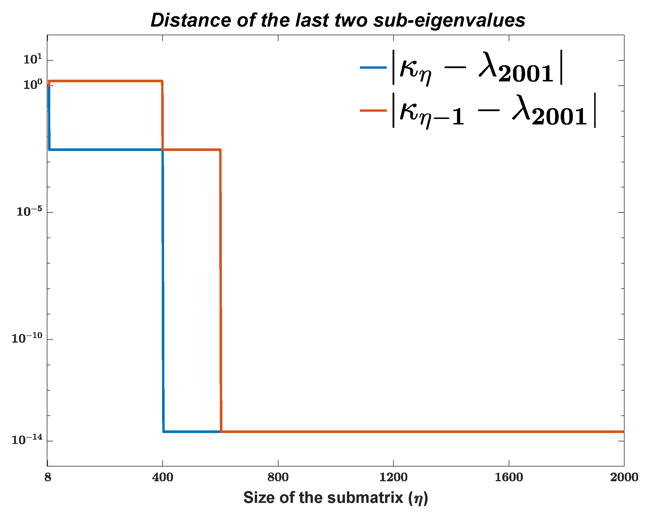
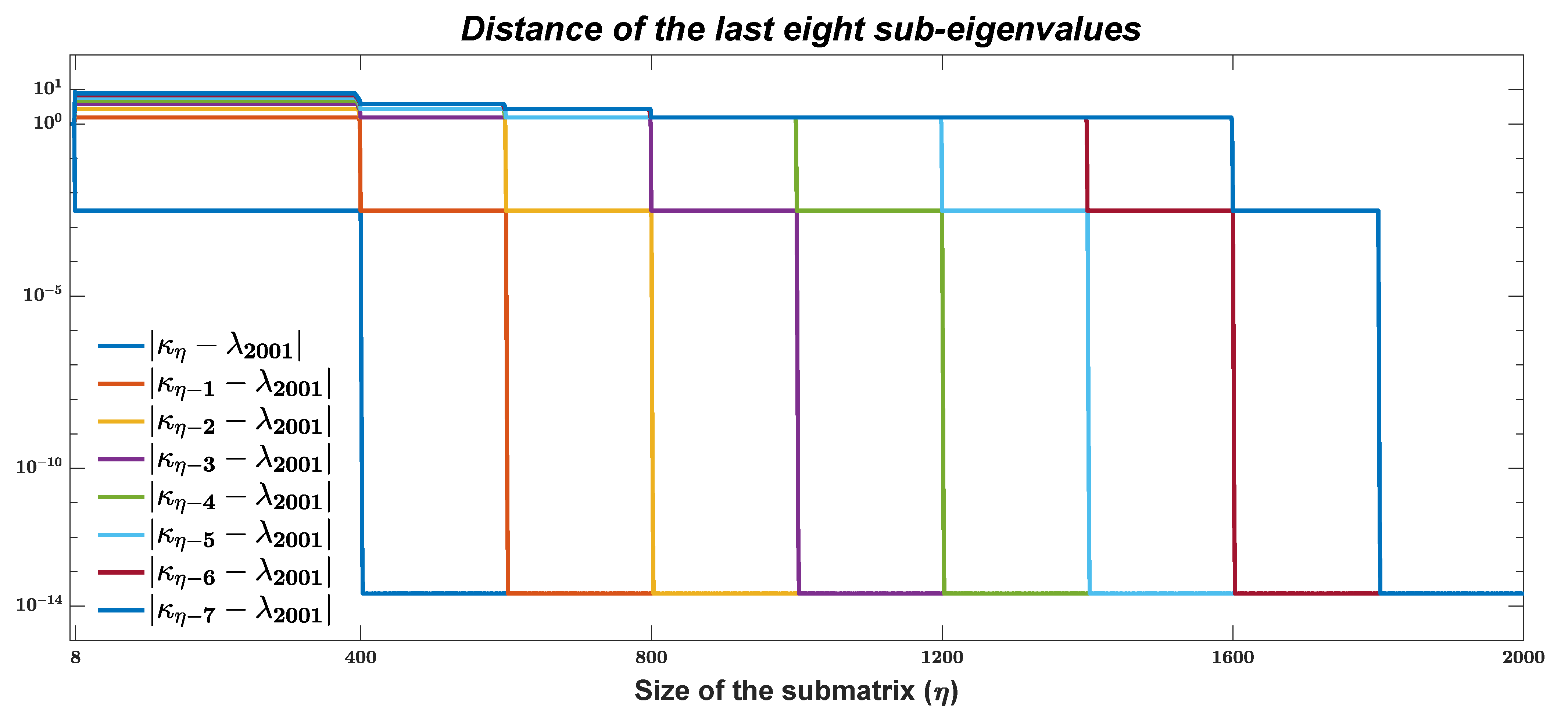
To illustrate Theorem 1 more intuitively, and as a complementary argument to the above proof, we performed the following numerical test. We calculated the distances between ${\lambda }_{2001}$ of $\Phi$ and the last two sub-eigenvalues of ${\Phi }_{1:\eta }(\eta \in [2,2000])$. Because by the Interlacing Property from [17], the close sub-eigenvalues to ${\lambda }_{2001}$ must be the last ones. The result is shown in Figure 2. A logarithmic scale on the y-axis has been used to emphasize the small entries. In Figure 2, ${\Phi }_{1:\eta }$ starts to have one close eigenvalue when $\eta >400$, which is the first low valley of the $|{\gamma }_k|$ curve, and two close eigenvalues when $\eta >600$, which is the second valley. We also present the results of the last eight sub-eigenvalues of ${\Phi }_{1:\eta }(\eta \in [8,2000])$ in Figure 3. It can be seen that, whenever ${\Phi }_{1:\eta }$ “crosses” a low valley of $|{\gamma }_k|$, the clustered sub-eigenvalues are one more. Figure 2 and Figure 3 confirm Theorem 1 well. See more and detailed numerical examples and results for accuracy in Section 6.

According to [13], we have that (recall $\mathcal{E}$ is the envelope vector from Lemma 1)

$$b_j\left|s_1\left(j\right)\right|\mathcal{E}(j+1)\approx V,$$

where V is independent of j. This means that a big $\mathcal{E}(j+1)$ corresponds to a small $|s_1\left(j\right)|$.

Therefore, our computation strategy of clustered eigenvalues is shown as follows:

1.

Every submatrix has one low valley of the $|{\gamma }_k|$ curve.

2.

The ends of the submatrix are the closest entries to the adjacent valleys.

3.

According to Lemma 2, $({\lambda }_p-{\lambda }_1)<p\sqrt{p}∥A∥ϵ$ ensures $∥T{\tilde{v}}_s∥<\sqrt{n}ϵ$, thus it can be used as the “clustering” threshold.

We show the method for computing severely clustered eigenvalues by the following pseudocode Algorithm 2.

Algorithm 2: Compute severely clustered eigenvalues.

Assume that the p valleys are arranged uniformly. The cost calculation of p severely clustered $\lambda$’s by Algorithm 2 is twice as large as the cost of one isolated $\lambda$ by Algorithm 1, while the Inverse Iteration method needs p times cost and a reorthogonalization. This means that Algorithm 2 saves time compared to the Inverse Iteration method even when disregarding its expensive orthogonal cost.

For the matrix $\Phi$, we calculated R’s (recall $R=∥Tz∥/∥z∥$, the residual norm) and the dot products of its last eight eigenvector approximations obtained by Algorithm 2. We show the mean and maximal results in

Table 1. Accuracy and orthogonality.

Method	Mean $\mathit{R}(\times \mathit{\epsilon }∥\mathit{\Phi }∥)$	Max $\mathit{R}(\times \mathit{\epsilon }∥\mathit{\Phi }∥)$	Mean Dot Product ($\times {\mathit{ϵ}}^{-1}$)	Max Dot Product ($\times {\mathit{ϵ}}^{-1}$)	Time Cost ($\times {10}^{-2}$ s)
Algorithm 2	1.5	1.5	0	0	0.1
Inverse Iteration	1.2	1.2	0	0.05	2.9
MRRR	1.2	1.2	0	0	4.2

and compare them to the results of the Inverse Iteration method and the MRRR method. The results were collected on an Intel Core i5-4590 3.3-GHz CPU and a 16-GB RAM machine. All codes were written in Matlab2017a and executed in IEEE double precision. The machine precision is $ϵ\approx 2.2\times {10}^{-16}$. It can be seen that all the eight eigenvector approximations are accurate and numerically orthogonal. See more examples and numerical results in Section 6.

4. Reorthogonalization

4.1. General Q Iteration

For severely clustered eigenvalues, Algorithm 2 saves considerable time and avoids reorthogonalization. However, if the group of clustering p eigenvalues has a close eigenvalue neighbor or another group of clustering eigenvalues with the distance $\in (p\sqrt{p}ϵ,{10}^{-3})∥A∥$ (note $p\sqrt{p}∥A∥ϵ$ is the threshold of severely clustering), Algorithm 2 can not ensure the orthogonality between them. Therefore, a reorthogonalization is needed. This is quite frustrating, not only because of the high cost of orthogonalization but also because using the modified Gram–Schmidt method for orthogonalization destroys the orthogonality of the eigenvectors obtained by Algorithm 2. In other words, the method we proposed in the previous section is meaningless. For example, two groups of severely eigenvalues have approximations $u_1$ and $u_2$, respectively, while $u_1-u_2<{10}^{-3}∥A∥$. Each group’s eigenvectors are orthogonal, but Algorithm 2 can not ensure the orthogonality of two from different groups. If one uses the modified Gram–Schmidt method to reorthogonalize them, it makes no difference whether the original vectors are orthogonal in groups. Therefore, we give a new reorthogonalization method in this section.

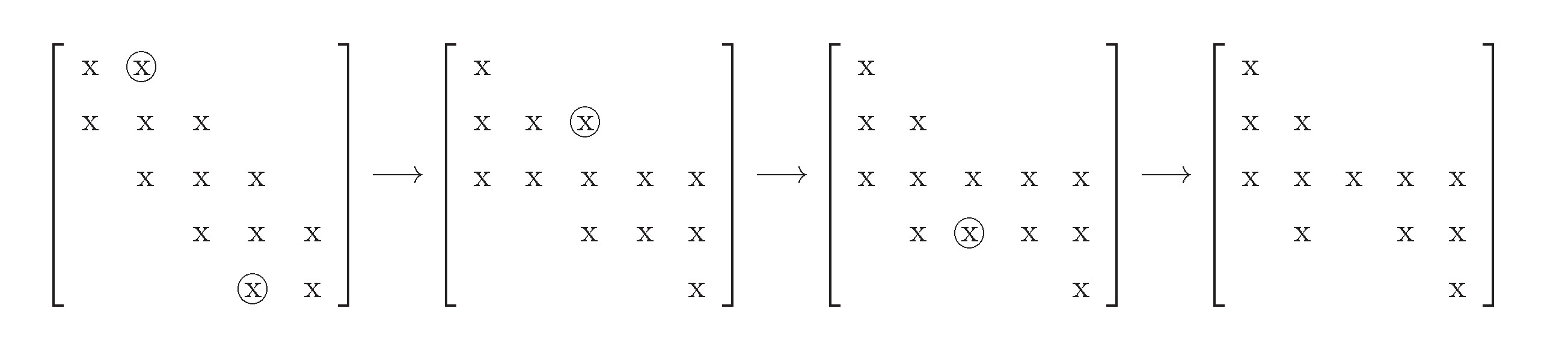
In [9], Dhillon introduced the twisted Q factorization. For an $n\times n$ ST matrix $T=A-{\lambda }_1$(${\lambda }_1$ is one eigenvalue of A) and a certain number $k(k\in [1,n\left]\right)$, implement the Givens rotation to its columns to eliminated $1\sim (k-1)$th components on its super-diagonal and $k\sim (n-1)$th components on the sub-diagonal. Finally, a singleton in the kth column is left. The process is shown in Figure 4 (from [9]), where $n=5$ and $k=3$.

Let W denote the final form of the twisted Q factorization, and we have

$$\begin{array}{cc}\hfill TQ& =W;\hfill \\ \hfill T& =W{Q}^T;\hfill \\ \hfill Q& =G_1{G}_2\dots G_{n-1},\hfill \end{array}$$

where $G_1\sim G_{n-1}$ are Givens rotation matrices. Obviously, $W_{k,k}=R_k$. Therefore, at least one k satisfies $\zeta =W_{k,k}\le \sqrt{n}ϵ$ according to Section 2.3.

Now, we introduce our so-called general Q iteration. For such a k that satisfies $\zeta \le \sqrt{n}ϵ$, we implement the corresponding Givens rotations to the rows of W. Using the example from Figure 4, the process is shown by

$$\begin{array}{c}{G}_1^{T}TQ=\left[\begin{array}{ccccc}\times & \times & & & \\ \times & \times & & & \\ \times & \times & \zeta & \times & \times \\ & \times & & \times & \times \\ & & & & \times \end{array}\right]\Rightarrow G_2^T\dots TQ=\left[\begin{array}{ccccc}\times & \times & & & \\ \times & \times & s_2\zeta & \times & \times \\ & \times & c_2\zeta & \times & \times \\ & \times & & \times & \times \\ & & & & \times \end{array}\right]\hfill \\ \Rightarrow G_3^T\dots TQ=\left[\begin{array}{ccccc}\times & \times & & & \\ \times & \times & s_2\zeta & \times & \times \\ & s_2\zeta & c_3{c}_2\zeta & \times & \times \\ & \times & -s_3{c}_2\zeta & \times & \times \\ & \times & & & \times \end{array}\right]\hfill \\ \Rightarrow G_4^T\dots TQ=\left[\begin{array}{ccccc}\times & \times & & & \\ \times & \times & s_2\zeta & \times & \times \\ & s_2\zeta & c_3{c}_2\zeta & -c_4{s}_3{c}_2\zeta & s_4{s}_3{c}_2\zeta \\ & \times & -c_4{s}_3{c}_2\zeta & \times & \times \\ & \times & s_4{s}_3{c}_2\zeta & \times & \times \end{array}\right]=Q^{T}TQ\hfill \end{array}$$

(11)

where $c_i$ and $s_i$ constitutes $G_i$, i.e.,

$$G_i:=\left[\begin{array}{cc}{c}_i& -s_i\\ s_i& c_i\end{array}\right].$$

Note that, in the last rotation of (11), the components on $(3,4)$ and $(3,5)$ have not changed. We obtain their values according to symmetry.

Finally, we have

$$A_1=Q^{T}TQ+{\lambda }_1$$

and complete one step of the general Q iteration. Obviously, $A_1$ has the same eigenpairs to A. As all $|c_i|$’s and $|c_i|$’s are less than 1, all the rest components of the kth rows and columns of $A_1$ are less than $\zeta$. Therefore, deflation can arise as

$$A_1=\left[\begin{array}{ccc}\times & \times & \\ \times & \times & & \times & \times & \\ & & {\lambda }_1& \\ & \times & & \times & \times & \\ & \times & & \times & \times & \end{array}\right]\Rightarrow \left[\begin{array}{cccc}\times & \times & & \\ \times & \times & \times & \times & \\ & \times & \times & \times & \\ & \times & \times & \times \end{array}\right]=B.$$

Thus, B has the numerical equal eigenvalues to ${\lambda }_2\sim {\lambda }_5$ and the corresponding eigenvectors can be calculated similarly to the QR method. For example, if $s_2={[x_1,x_2,x_3,x_4]}^T$ is the eigenvector of B with respect to ${\lambda }_2$, then $v_2=Q{s}_2$. These $v_i$’s are certainly orthogonal. Note that B can be transferred to an ST matrix by chasing and eliminating its bulge (for example, the $(2,4)$ and (4, 2) components of B) with Givens rotations. Therefore, it costs at most 1.5 times operations compared to the QR (or QL) iteration, which is the exceptional case when $k=n$ or 1.

Therefore, the general Q iteration is to fulfill a deflation of a certain $\lambda$ by QR-like transformation. For a normal ST matrix and one accurate approximation to $\lambda$, $k=1$ or n is enough. Thus, the cost of chasing the bulge can be saved. However, in some special cases, $|{\gamma }_1|$ or $|{\gamma }_n|$ can both be small, which means it costs numerous QR-like iterations to converge. This is similar to the solution of (2) by inverse iterations, considering the strong relationship between the Inverse Iteration method and the QR (or QL) method [7]. Recall that we give the one-step inverse iteration in Section 2, and the general Q iteration can be regarded as a one-step QR-like iteration. In our numerical experience, the case that several QR iterations (which use an accurate eigenvalue approximation as the shift) can not obtain convergence is not rare. For example, for a random $2000\times 2000$ ST matrix, its most ${\lambda }_i$’s can ensure one-step converges by QR iteration, but some ${\lambda }_i$’s may cost more than 50 steps. In addition, this case almost arises in every random matrix.

Mastronardi and Van Dooreen discovered this instability when obtaining an ST eigenvector and solved the problem by a modified implicit QR decomposition method [12]. Their method can ensure an accurate calculation. However, this paper uses a modified inverse iteration method to calculate the eigenvector. The implicit QR decomposition in our paper is used for deflation and guarantee of orthogonality in the case that the eigenvalues cluster generally.

The corresponding pseudocode for computing generally clustered eigenvectors is given in Algorithm 3. The generally clustering denotes that the span of the p clustered eigenvalues is not big enough to guarantee orthogonality of its corresponding eigenvectors (calculated by the Inverse Iteration method or Algorithms 1 and 2), i.e., ${\lambda }_p-{\lambda }_1\le {10}^{-3}∥A∥$.

Algorithm 3: Computing generally clustered eigenvectors.

4.2. Cost of Reorthogonalization

This subsection concerns the cost of reorthogonalization in Algorithm 3. For k clustered eigenvalues, the last obtained v (line 7 in Algorithm 3) is a $(n+1-k)\times 1$ vector. v has to be premultiplied $n-k$ Givens rotation matrices to transfer to $(n+2-k)\times 1$. Repeat this process until the length reaches n. For every Givens rotation, the cost is six operations. Therefore, the total cost is

$$\begin{array}{cc}\hfill & 6\times \left(\right(n-k)\times 1+(n+1-k)\times 2+(n+2-k)\times 3+\dots +(n-2)\times (k-1\left)\right)\hfill \\ \hfill & =6\times n\times (1+2+\dots +k-1)-6\times (k\times 1+(k-1)\times 2+\dots +2\times (k-1\left)\right)\hfill \\ \hfill & =3n{k}^2-\left(k^3+3k^2-4k+3n\right).\hfill \end{array}$$

(12)

At first sight, (12) is hardly satisfactory, as the modified Gram–Schmidt method costs only $4n\times (1+2+3+\dots +k)=2n{k}^2$ operations. Only when k is close to n, our method matches the efficiency of the modified Gram–Schmidt method. Moreover, those cases where we need to use the general Q iteration (the QR-like iterations cannot converge at one step) have not been considered. However, the cost will slump for cases with many severely clustered eigenvalues within groups.

For example, if m eigenvalues are severely clustered among the k eigenvalues, the cost is

$$3n{(k-m)}^2-\left({(k-m)}^3+3{(k-m)}^2-4(k-m)+3n\right)+6(n-m)m,$$

(13)

which decreases from $O\left(n{k}^2\right)$ to $O\left(nk\right)$ if m is close to k. In addition, the cost for the modified Gram–Schmidt method, in this case, is $4n(m+m+1+\dots +k)=2n(m+k)(k-m)$.

If the k eigenvalues can be divided into two severely clustering groups, the cost is

$$6(n-m)m,$$

(14)

which decreases from $O\left(n{k}^2\right)$ to $O\left(nm\right)$. In addition, the cost for the modified Gram–Schmidt method, in this case, is $2n(m+k)(k-m)$.

Therefore, Algorithm 3 calls the deflation method with the general Q iteration or the modified Gram–Schmidt method according to an advanced prediction by (12)–(14). However, both methods are time-consuming in cases where k is very close to n, and the eigenvalues have few severely clustering groups. In this case, the best method is the MRRR method. See more examples and numerical details in Section 6.

4.3. Modification of QR-Like Iteration

The general Q iteration can be seen as starting a QL iteration from the left of the matrix, stopping it at column k, and then doing a QR iteration from the right of the matrix till there is a singleton in the kth column. We give a subtle modification to the QR or QL iteration with the implicit shift to save some operations. Take the QR iteration as an example, and the traditional process is shown in Algorithm 4.

One step of QR iteration implemented into a $4\times 4$ ST matrix is shown as follows:

$$\begin{array}{c}\begin{array}{c}\left[\begin{array}{cc}{c}_1& s_1\\ -s_1& c_1\end{array}\right]\\ \begin{array}{c}\\ \end{array}\end{array}\left[\begin{array}{cccc}{a}_1& b_1& & \\ b_1& a_2& b_2& \\ & b_2& a_3& b_3\\ & & b_3& a_4\end{array}\right]\begin{array}{c}\left[\begin{array}{cc}{c}_1& -s_1\\ s_1& c_1\end{array}\right]\\ \begin{array}{c}\\ \end{array}\end{array}\hfill \\ \Rightarrow \left[\begin{array}{cccc}\times & \times & s_1{b}_2& \\ -s_1\delta & {\pi }_2+c_1\delta & c_1{b}_2& \\ & b_2& a_3& b_3\\ & & b_3& a_4\end{array}\right]\begin{array}{c}\left[\begin{array}{cc}{c}_1& -s_1\\ s_1& c_1\end{array}\right]\\ \begin{array}{c}\\ \end{array}\end{array}\hfill \\ \Rightarrow \left[\begin{array}{cccc}{\overline{a}}_1& s_1{\pi }_2& s_1{b}_2& \\ s_1{\pi }_2& c_1{\pi }_2+\delta & c_1{b}_2& \\ s_1{b}_2& c_1{b}_2& a_3& b_3\\ & & b_3& a_4\end{array}\right]\hfill \end{array}$$

(15)

Algorithm 4: QR iteration with the implicit shift.

In (15), ${\pi }_{i+1}$ is updated by ${\pi }_{i+1}=c_i(a_{i+1}-\delta )-s_i{b}_i$, which corresponds to line 10 in Algorithm 4. This equation can be rewritten as

$$\begin{array}{cc}\hfill {\pi }_{i+1}/c_i& =(a_{i+1}-\delta )-s_i{b}_i/c_i\hfill \\ \hfill & =(a_{i+1}-\delta )-b_i{c}_{i-1}{b}_i/{\pi }_i\hfill \\ \hfill & =(a_{i+1}-\delta )-b_i^2/({\pi }_i/c_{i-1})\hfill \end{array}$$

Without loss of generality, assume that $c_0=1$, then ${\pi }_1/c_0=a_1-\delta =q_1$ (recall $q_i$ is the Sturm sequence from (8)). Finally, we have

$${\pi }_{i+1}/c_i=q_{i+1}(i\in [0,n-1]).$$

(16)

Note all the $q_i$’s have been calculated in advance when searching the smallest $|{\gamma }_k|$ in our methods; thus, we can use (16) to update $\pi$’s instead. We show the modified QR iteration algorithm in Algorithm 5.

Algorithm 5 costs $6n$ multiplications, $2n$ divisions, and $(n-1)$ square roots while Algorithm 4 costs $9n$ multiplications, $2n$ divisions, and $(n-1)$ square roots. Thus, our modification saves $3n$ multiplications.

Algorithm 5: Modified QR iteration with the implicit shift.

5. Avoiding Overflow and Underflow

Our new method obtains an eigenvector essentially by the cumulative products of q’s, as shown in lines 9 and 12 of Algorithm 1. As is well known, the products can grow or decay rapidly; hence, the recurrences to compute them are susceptible to severe overflow and underflow problems. This section gives a relatively cheap algorithm to avoid overflow and underflow.

Let f denotes the overflow threshold, for example, $f=2^{1023}$ in IEEE double precision arithmetic. Whenever one intermediate product during the recurrences exceeds f, multiply it by $f^{-1}$ to normalize and continue the iteration. Similarly, whenever one $\le f^{-1}$, multiply it by f. At the same time, we save the corresponding entry and mark 1 for overflow and $-1$ for underflow.

Assume y positions, which divide the eigenvector approximation $\tilde{v}$ into $y+1$ parts, are marked when the iteration is completed. Then, we have a $y\times 1$ vector Y, with components of 1’s and $-1$’s. For any certain position, the mark 1 means the components of $\tilde{v}$ from it to the end are shrunk by a factor of f compared to v. In addition, the mark $-1$ means amplification by f. The mark before the first component of $\tilde{v}$ is zero. Thus, we have $Y\leftarrow [0;Y]$.

Calculate the cumulative sums of Y from the first component to everyone and save the results at each entry. In this way, each component of Y corresponds to each part of $\tilde{v}$, and its value represents the specific degree to which the corresponding part has been enlarged or reduced. A positive value of m means that this part has been reduced by $f^m$ times, while a negative value means enlarged. The corresponding part is not enlarged or reduced when the value is zero.

Revisiting $\tilde{v}$, all the components have not overflowed but are just to be restored to their true values. In addition, the biggest part after restoration corresponds to the biggest component of Y (recall each component of Y corresponds to each part of $\tilde{v}$) because it is reduced by the most significant times. Since $\tilde{v}$ is ultimately normalized, we take the biggest part as the benchmark. Thus, the second biggest component of Y corresponds to the second biggest part of $\tilde{v}$ after restoration, which should be divided by f. The rest parts, if they exist, need to be divided by $f^2$ or more, thus directly taking zeros as its components.

We give the corresponding pseudocode in Algorithm 6, which corresponds to the details of lines 9 and 12 of Algorithm 1.

Algorithm 6: Compute $\prod q$ without overflow and underflow.

    Finally, we give the complete modified Inverse Iteration method by Algorithm 7.

Algorithm 7: Modified Inverse Iteration method.

6. Numerical Results

In this section, we present a numerical comparison among the modified Inverse Iteration method and four other widely used algorithms for computing eigenvectors:

1.

the Inverse Iteration method, by calling subroutine “dstein” from LAPACK in Matlab;

2.

the MRRR method, by calling subroutine “dstegr” from LAPACK in Matlab;

3.

the QR method, by calling subroutine “dsteqr” from LAPACK in Matlab;

4.

the DC method, by calling subroutine “dstedc” from LAPACK in Matlab.

Since the MRRR, QR, and DC methods compute the eigenpairs instead of only eigenvectors, we compared the total cost for eigenpairs in this section. To obtain eigenvalues for Algorithm 7 and the Inverse Iteration method, we use the PWK version of the QR method (by calling subroutine ‘dsterf’ from LAPACK in Matlab) when calculating more than $5\%$ eigenpairs, otherwise use the Bisection method (by calling subroutine ‘dstebz’ from LAPACK in Matlab). Note the QR and DC methods are only available when computing all the eigenpairs and thus will not be compared in the cases when computing parts of the eigenpairs.

We use the following five types of $n\times n$ matrices for tests:

1.

Matrix ${\Phi }_1$, which is constructed similarly to $\Phi$ in Section 3 with ${\alpha }_0=$ (1:200). We change the repeat times of $\alpha \leftarrow [\alpha ;{\alpha }_0]$ to adjust the size of Matrix ${\Phi }_1$. Note this matrix has many groups of clustered eigenvalues (severely and generally clusterings both exist) and has overflow issues if calculated directly.

2.

Matrix ${\Phi }_2$, which is constructed similarly to ${\Phi }_1$ with ${\alpha }_0=$ (1:80). This matrix also has many groups of clustered eigenvalues (severely and generally clusterings both exist) but has no overflow issue if calculated directly.

3.

Matrix $W_1$, the famous Wilkinson matrix, which has the ith diagonal component equal to $\left|\right(n+1)/2-i|$(n is odd) and all off-diagonal components equal to 1. All its eigenvalues severely cluster in pairs.

4.

Matrix $W_2$, another form of the Wilkinson matrix, which has the ith ($i\in [1,(n+1)/2]$) diagonal component equal to $\left|\right(n+1)/2-i|$(n is odd), the ith ($i\in \left[\right(n+1)/2+1,n]$) diagonal component equal to $-\left|\right(n+1)/2-i|$ and all off-diagonal components equal to 1. Its eigenvalues do not cluster if the size is less than 2000.

5.

Random Matrix with both diagonal and off-diagonal elements being uniformly distributed random numbers in [−1, 1]. Note that all the Random Matrix results in this section are mean data of 20 times tests.

The results were collected on an Intel Core i5-4590 3.3-GHz CPU and 16-GB RAM machine. All codes were written in Matlab2017a and executed in IEEE double precision. The machine precision is $ϵ\approx 2.2\times {10}^{-16}$.

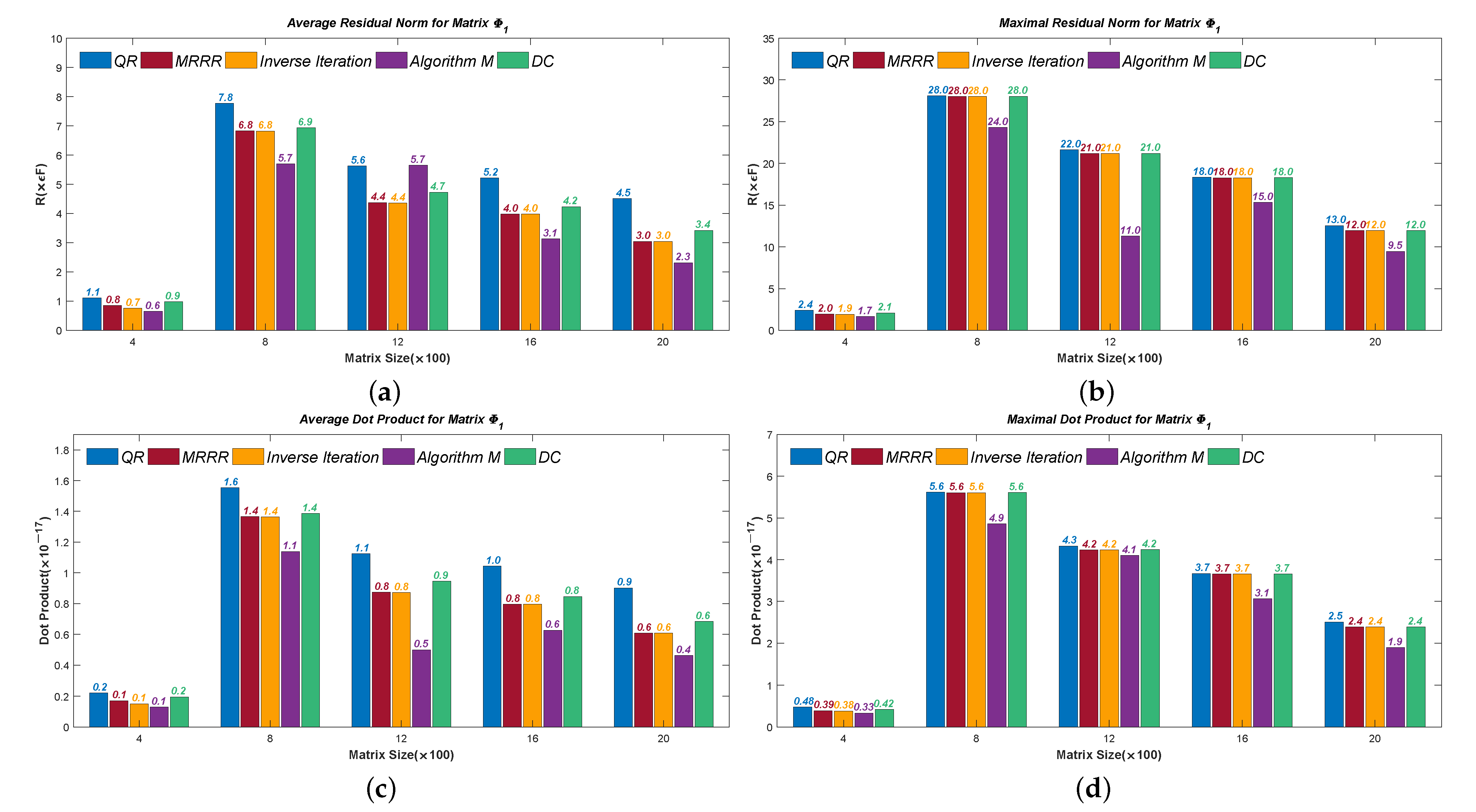
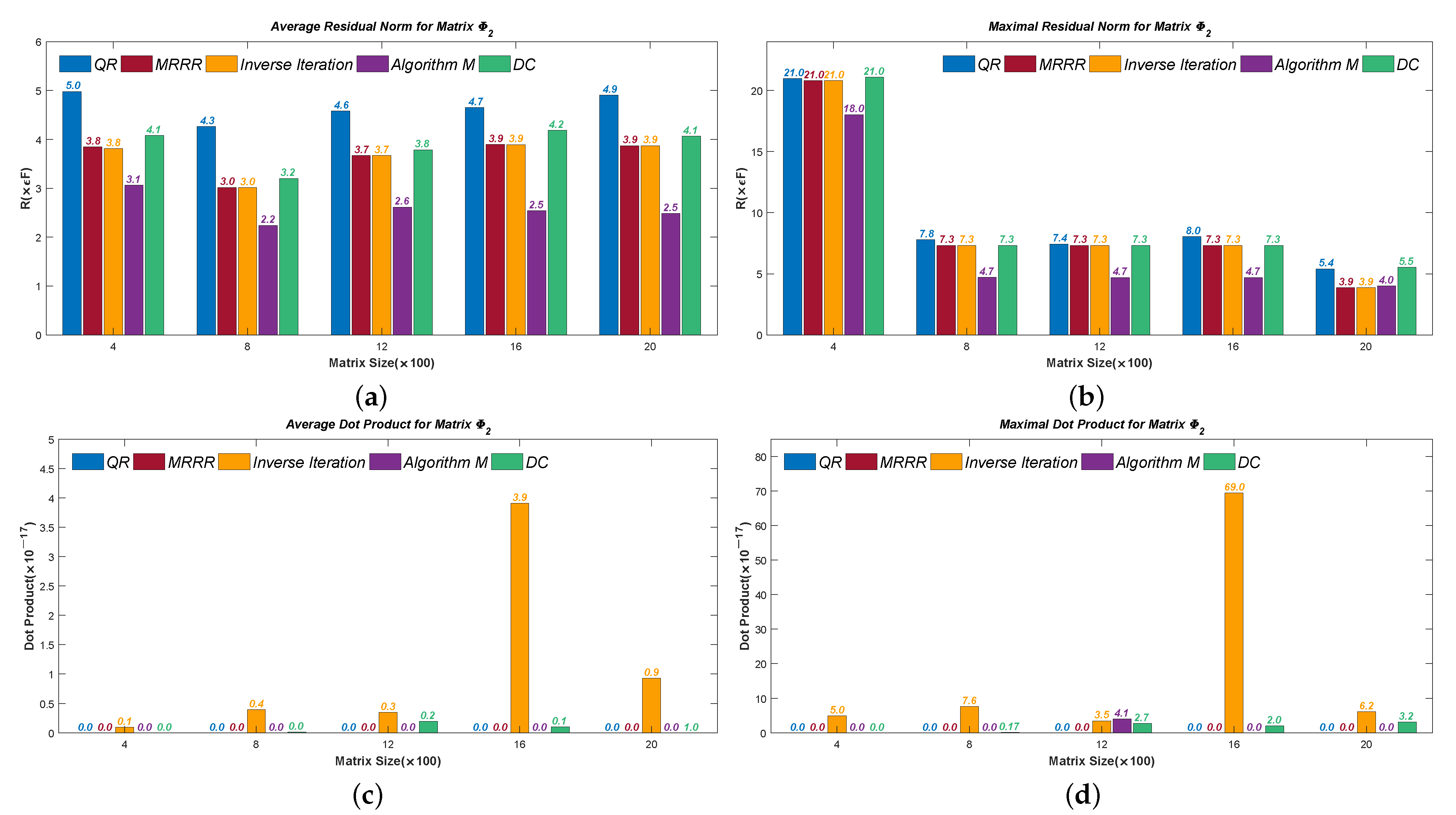
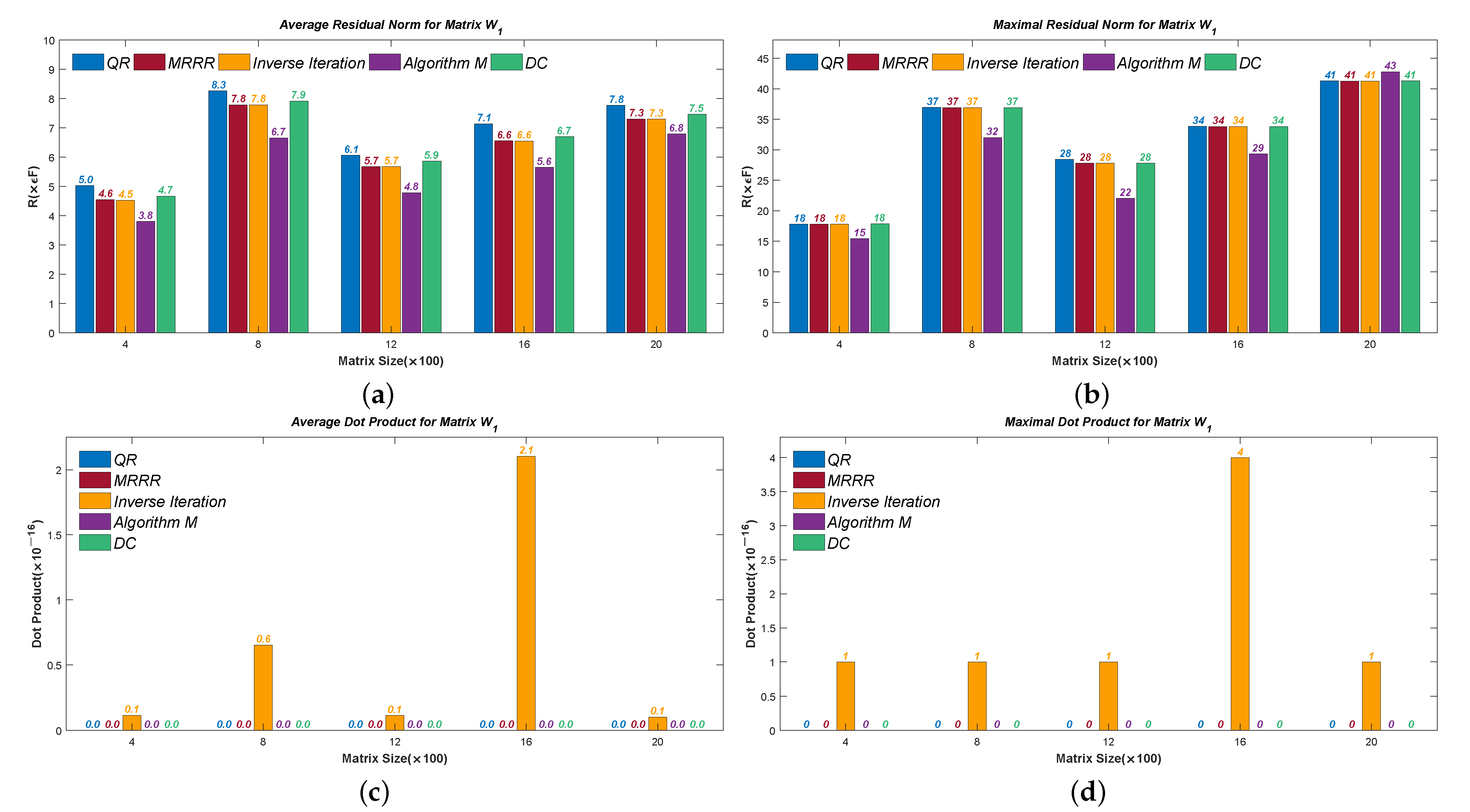
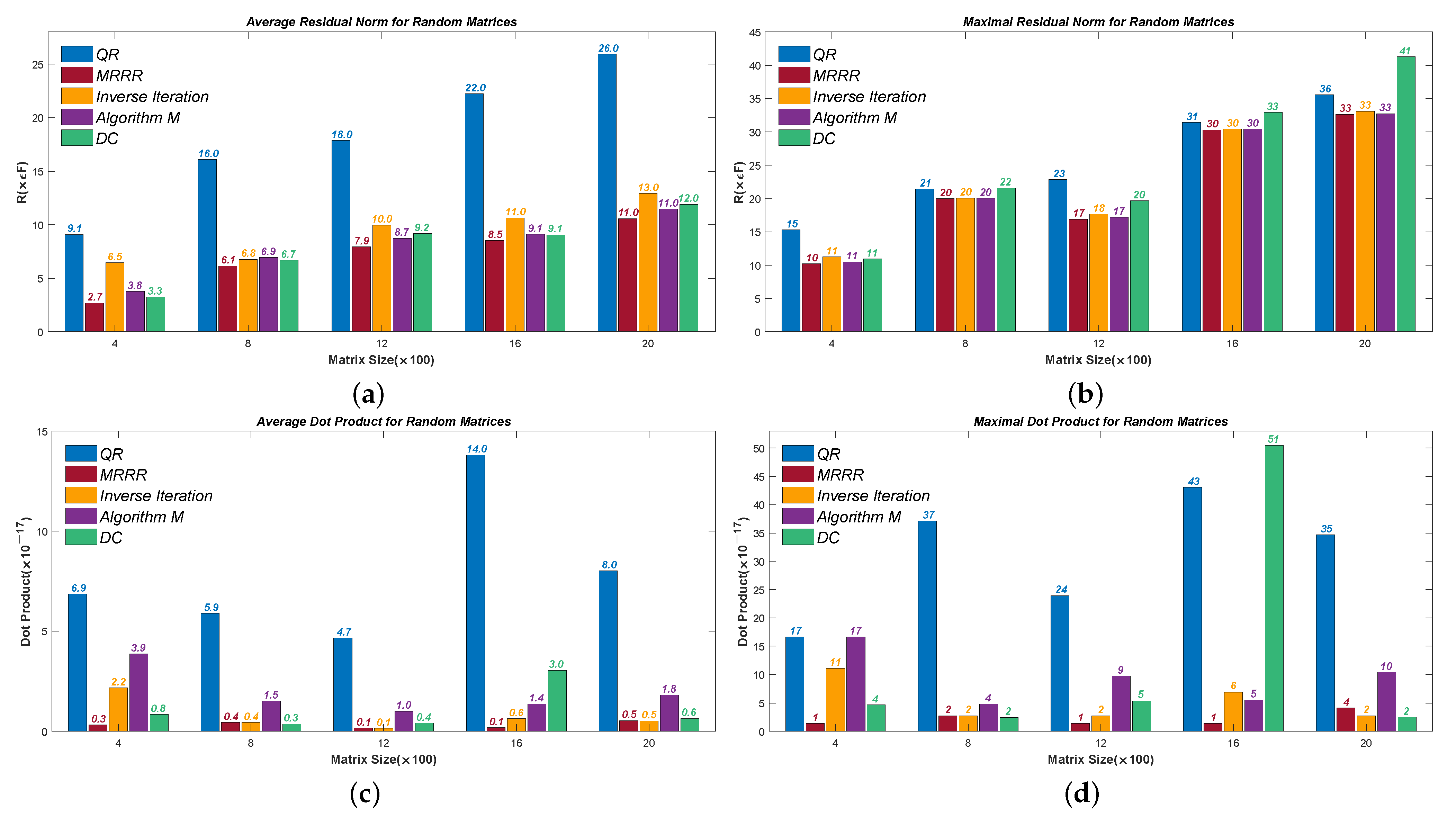
6.1. Accuracy Test

Figure 5, Figure 6, Figure 7, Figure 8 and Figure 9 present the results of the residual norms, i.e., $R=T\tilde{v}/∥v∥$, where the Average Errors denote the means of R’s of all the calculated eigenvectors and the Maximal Errors denote the maximum. The results of dot products of the calculated eigenvectors are also presented to show orthogonality. Different sizes are used in our test, from $400\times 400$ to $2000\times 2000$. We denote the corresponding 2-norm of the tested matrix, for example, $F=∥{\Phi }_1∥$ in Figure 5. The results confirm that Algorithm 7 computes accurate and numerical orthogonal eigenvectors.

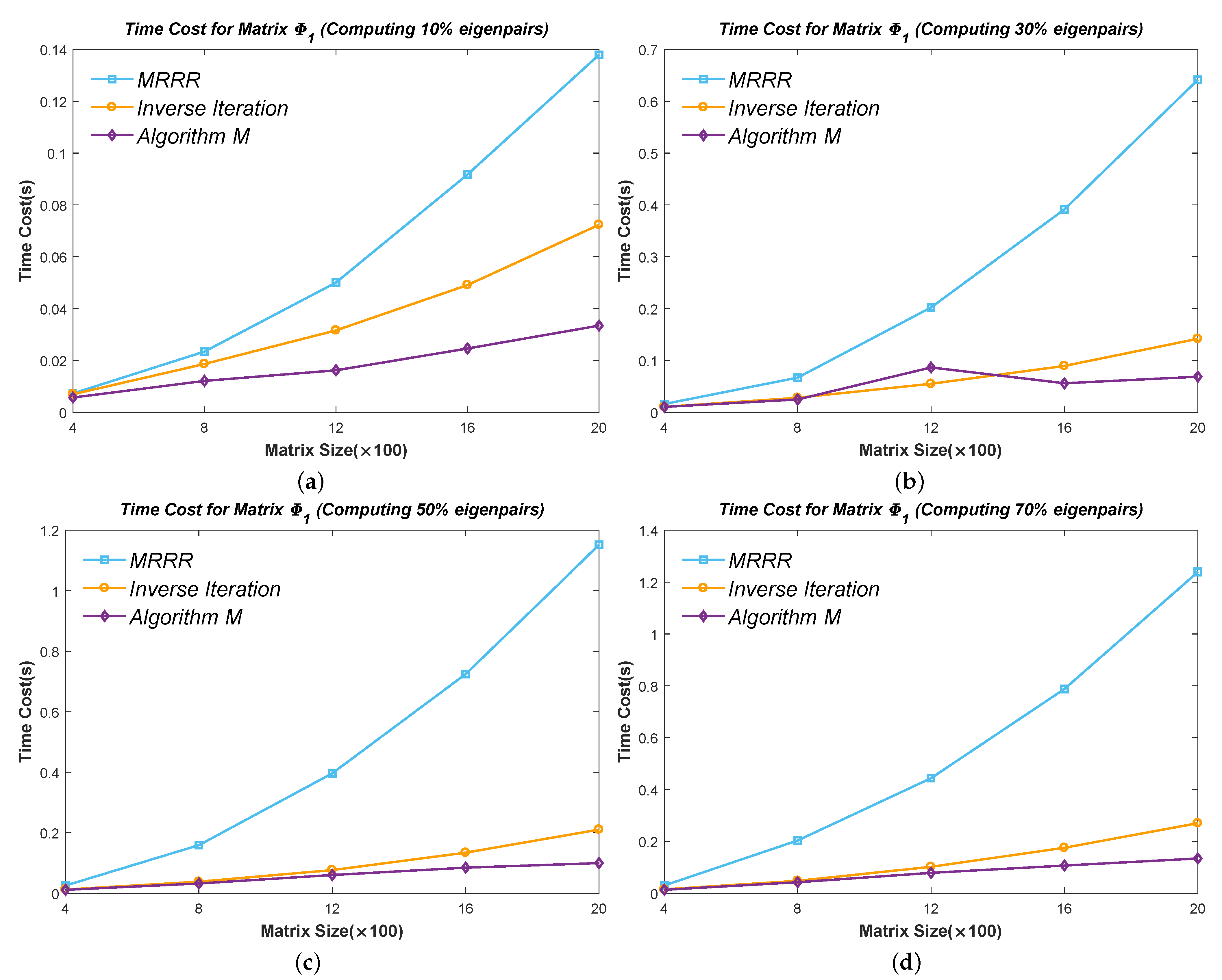
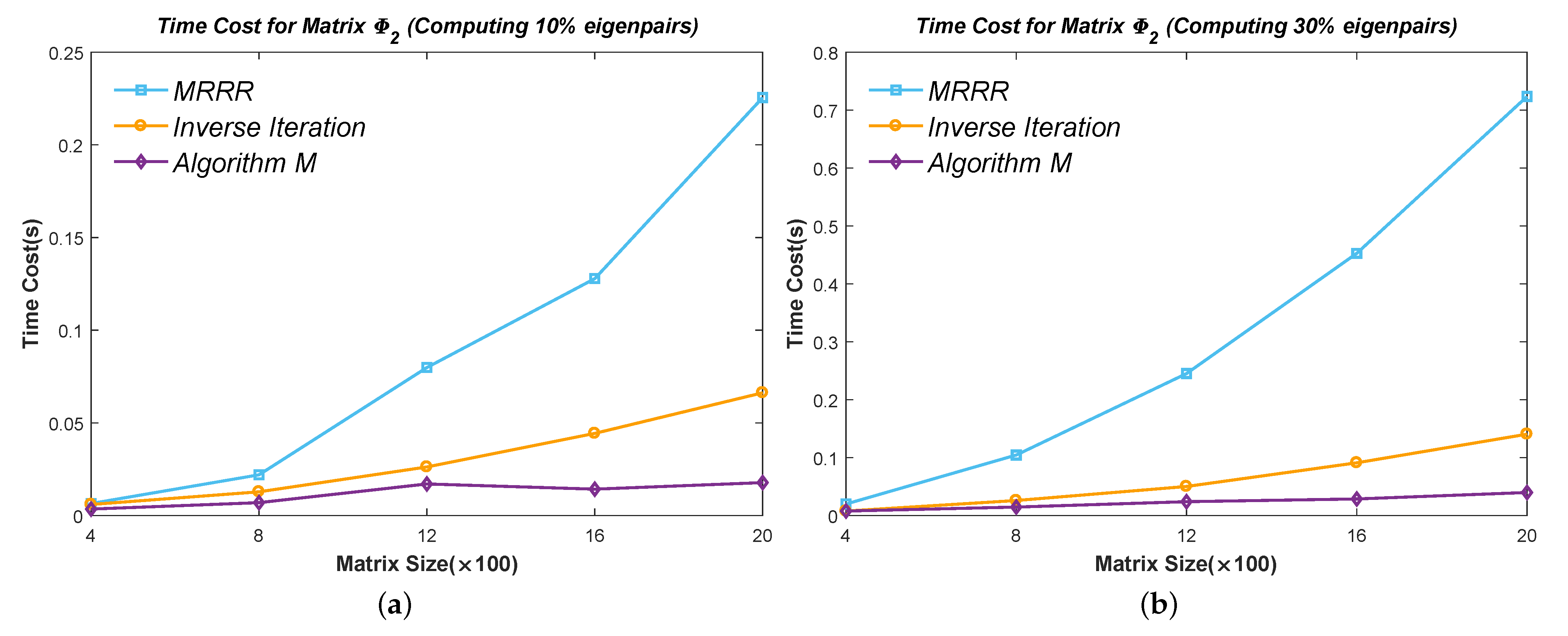
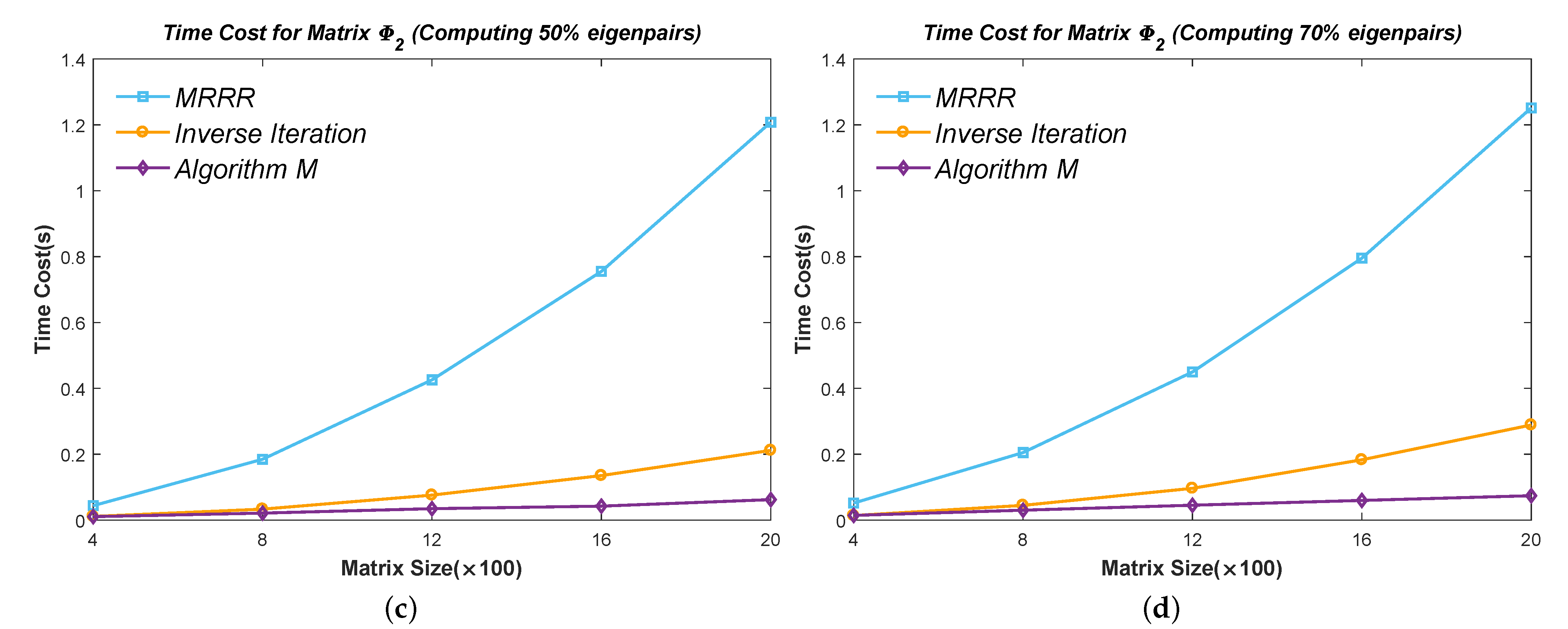
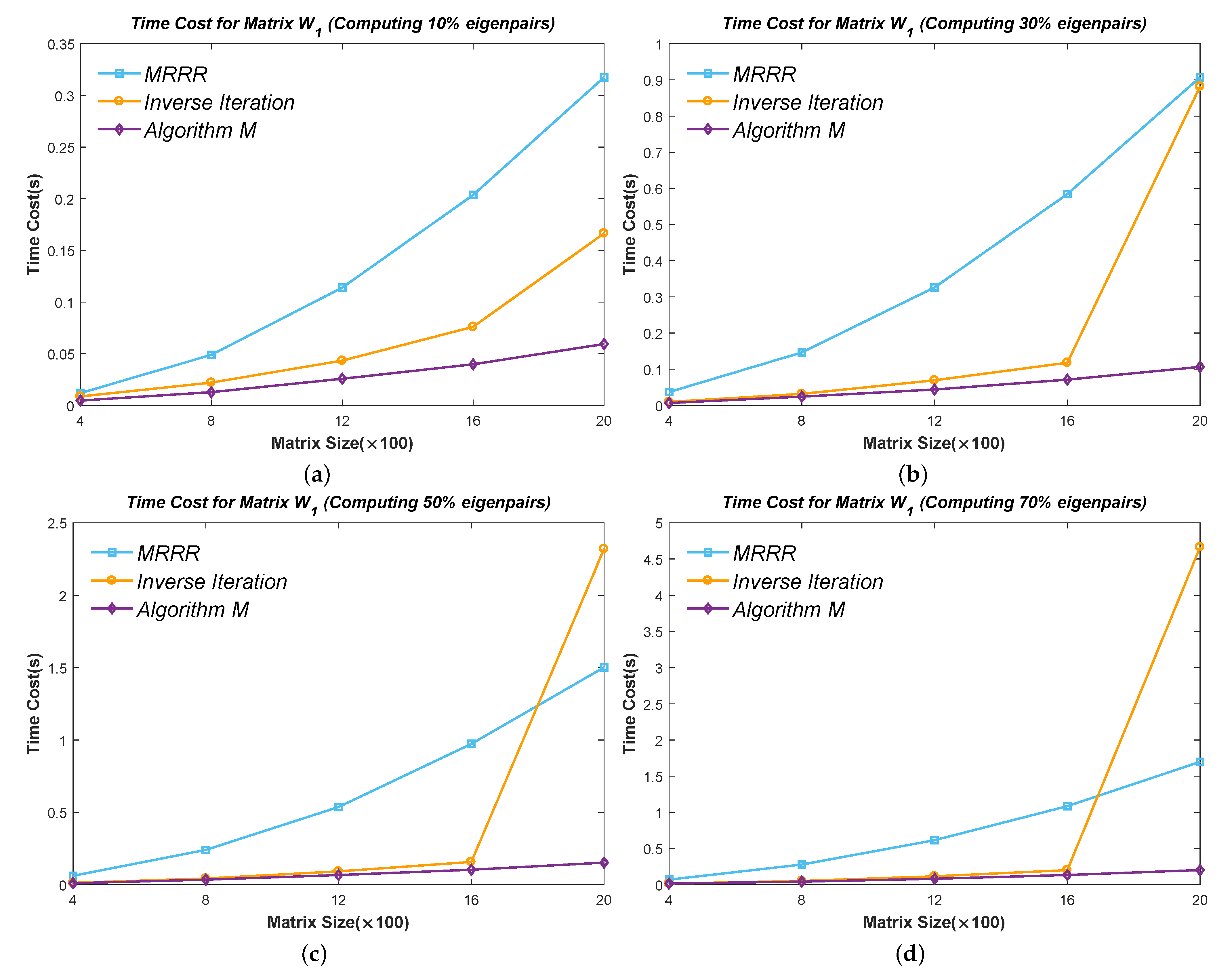
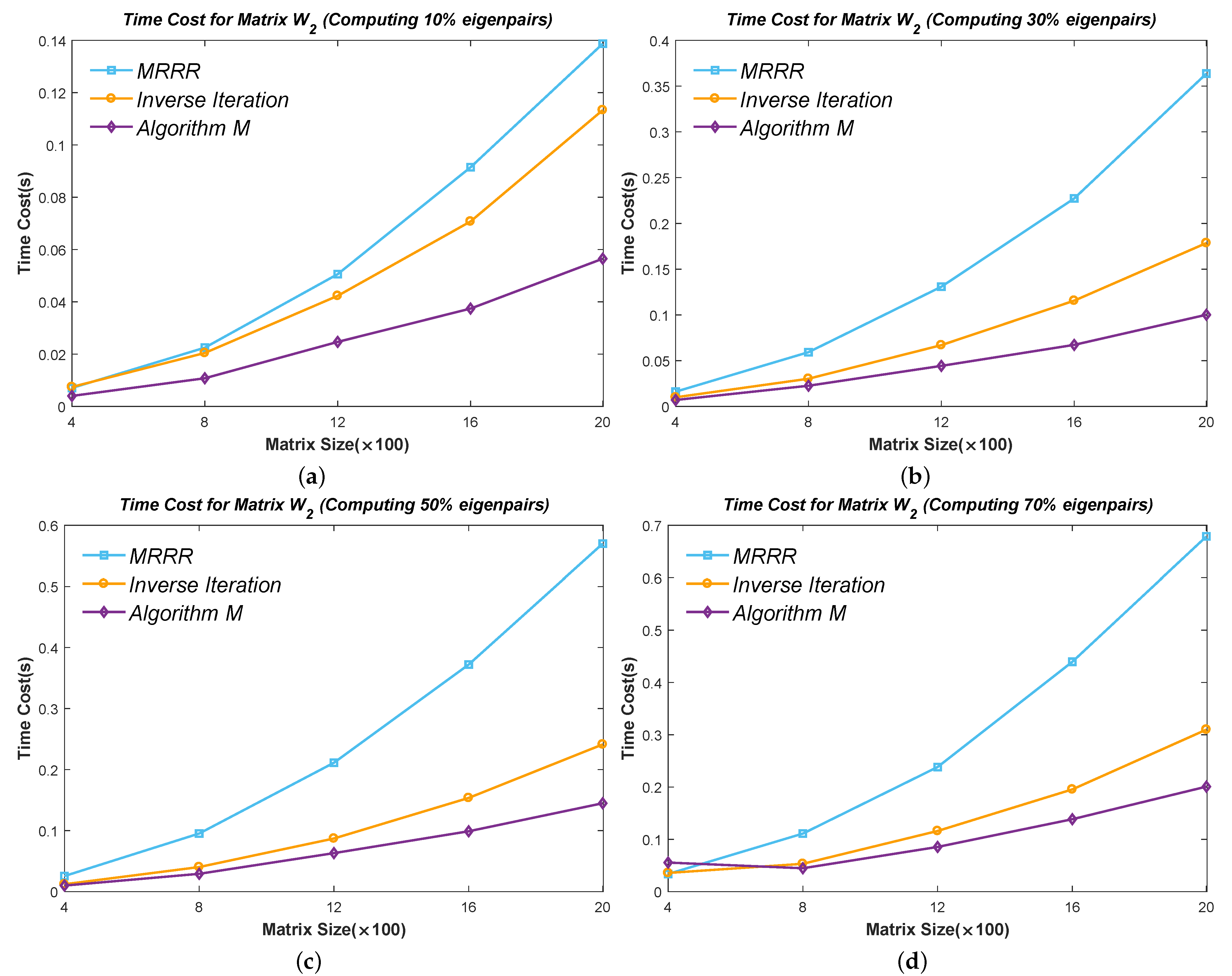
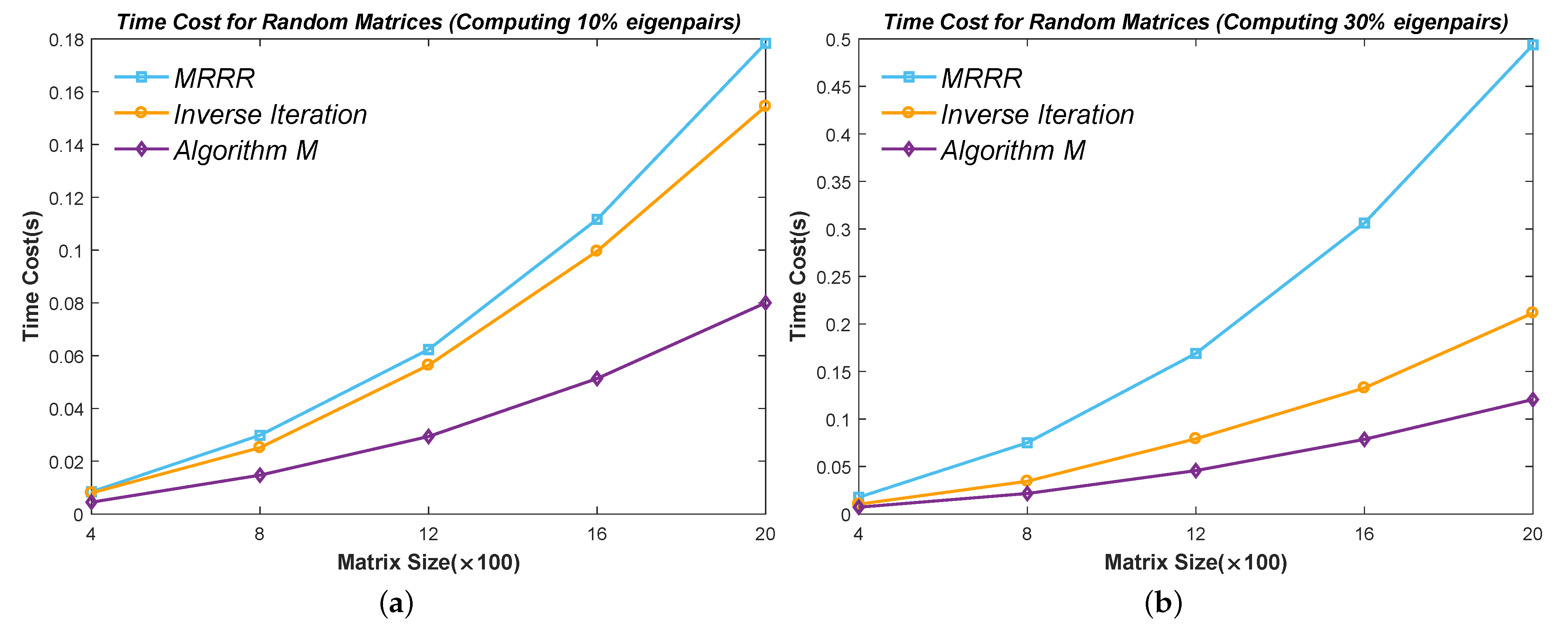
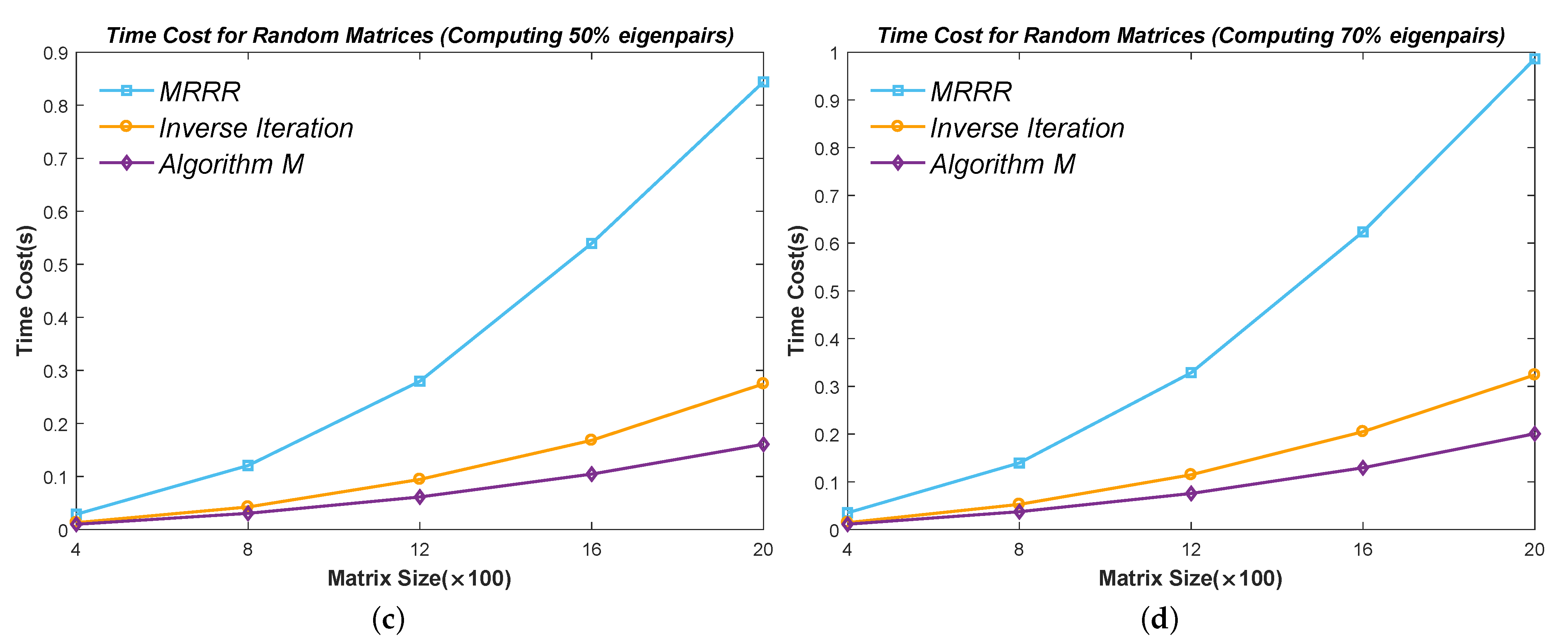
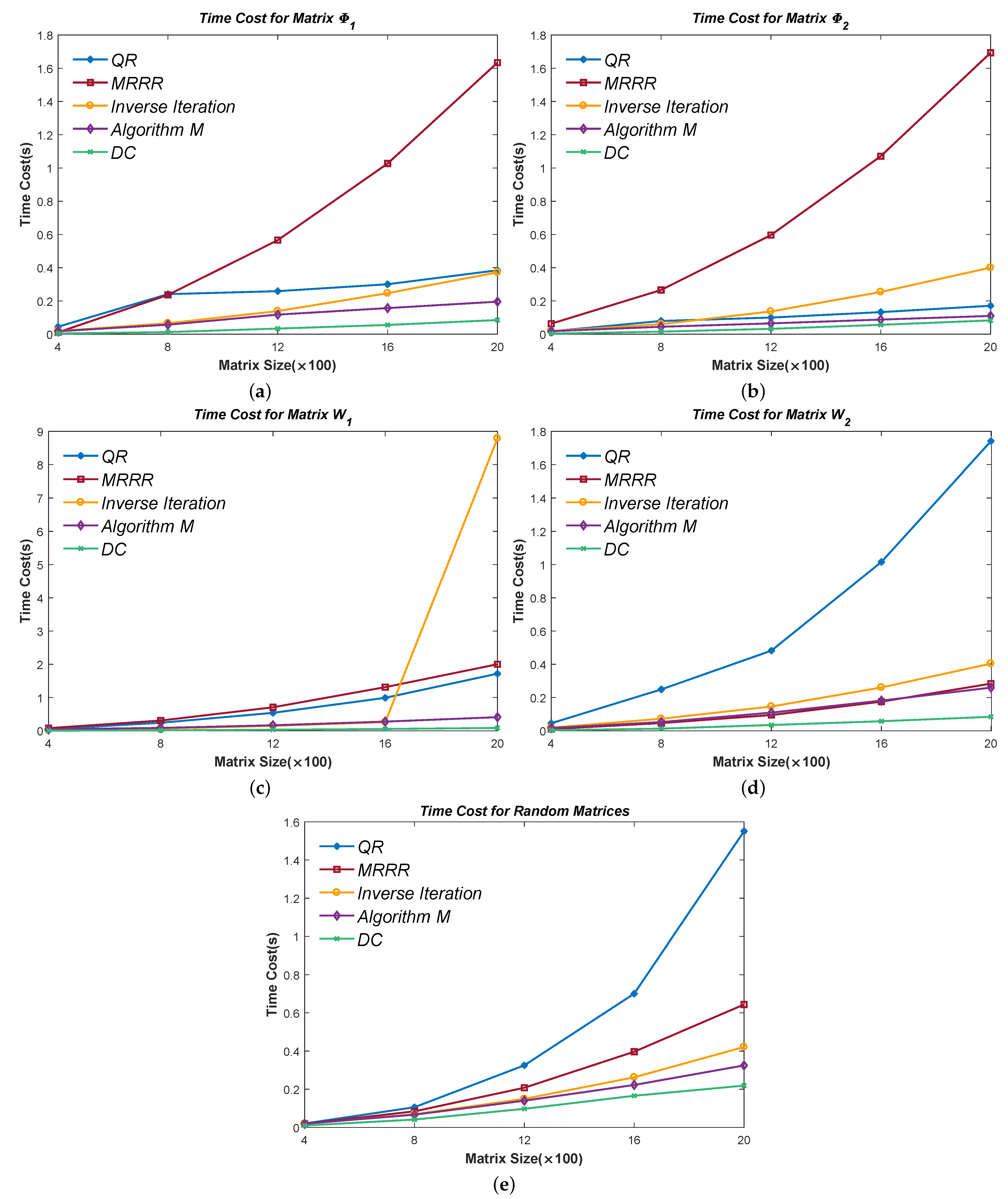
6.2. Efficiency Test of Part Eigenpairs

Figure 10, Figure 11, Figure 12, Figure 13 and Figure 14 show the time cost for computing $10\%$, $30\%$, $50\%$, and $70\%$ eigenpairs of the above five types of matrices in each size. Note the cost of the Inverse Iteration method surges in Figure 12 because the eigenvalues start to cluster and need an expensive reorthogonalization by the modified Gram–Schmidt method as the size of Matrix $W_1$ rises. The MRRR method costs the most in every matrix because it needs more accurate eigenvalues and calls the Bisection method, while the Inverse Iteration and Algorithm 7 call the PWK version of the QR method to obtain all eigenvalues. Finally, the results show that the modified Inverse Iteration method always costs the least time and has a surpassing efficiency when eigenvalues severely cluster, which confirms our points in Section 3.

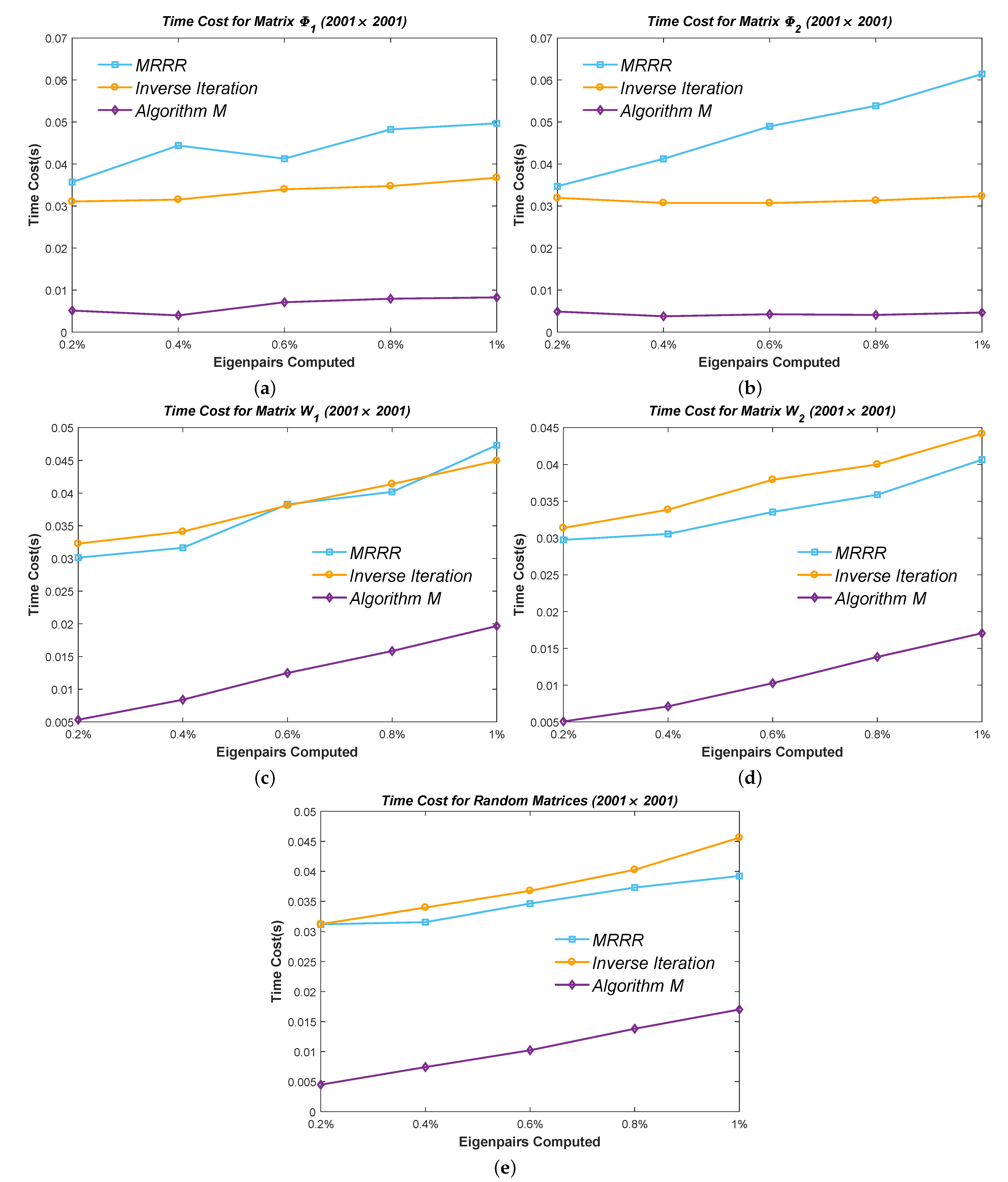
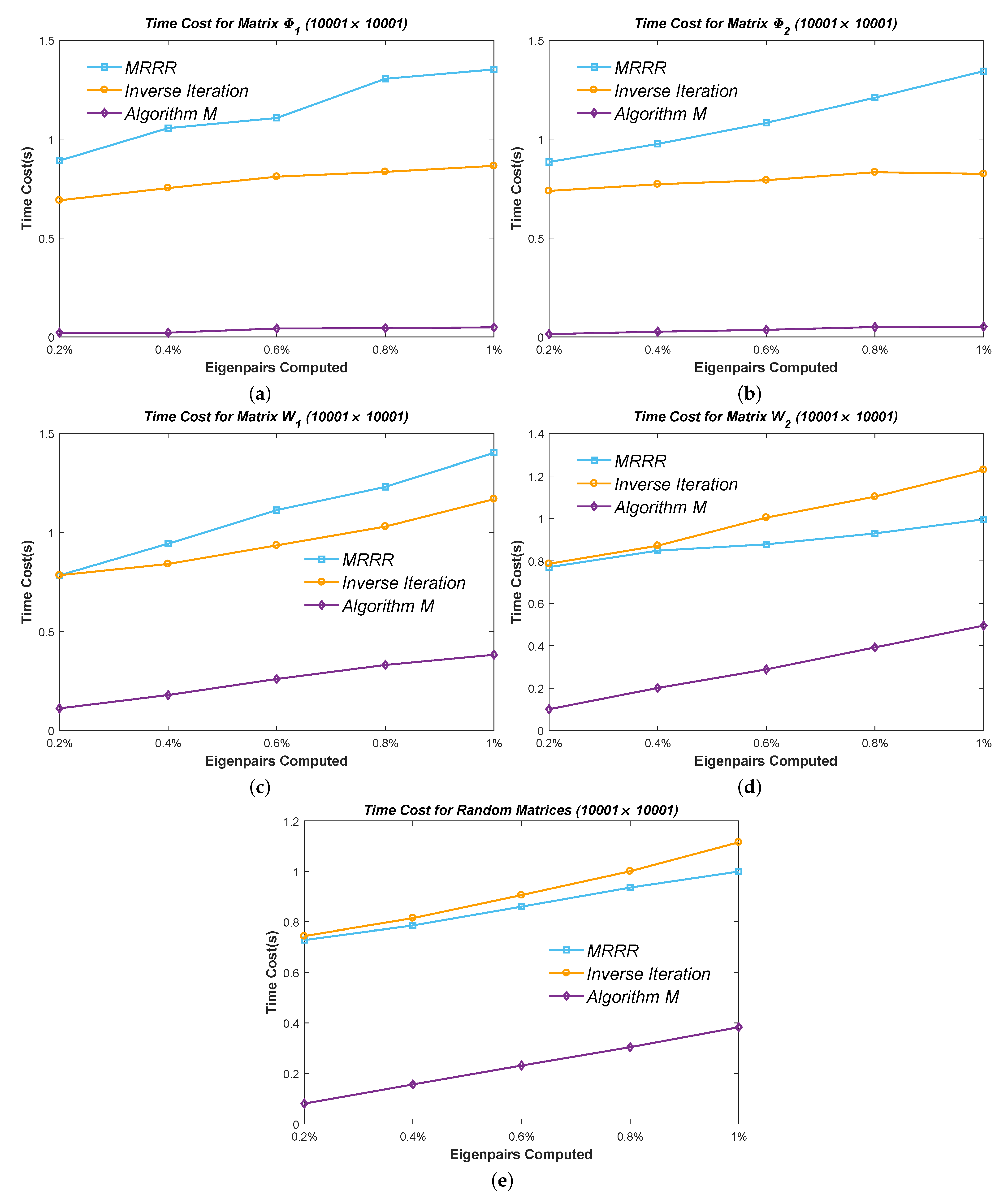
6.3. Efficiency Test of Minor Eigenpairs

When it comes to a minor set of eigenpairs, it is inadvisable to calculate all the eigenvalues by the PWK version of the QR method for the Inverse Iteration and Algorithm 7. We use the Bisection method instead, similar to the MRRR algorithm. Thus, the result is more convictive in this case because all the methods obtain the eigenvalues at an identical cost.

We calculated $0.2\%$, $0.4\%$, $0.6\%$, $0.8\%$, and $1\%$ eigenpairs of the above five types of matrices and used two sizes: $2001\times 2001$ and $10001\times 10001$. The results are presented in Figure 15 and Figure 16. It can be seen that the cost of the MRRR method is close to the Inverse Iteration method when computing clustered eigenpairs but higher in other cases. Once again, the modified Inverse Iteration prevails in all cases.

6.4. Efficiency Test of All Eigenpairs

As discussed in previous sections, Algorithm 7 is not suitable for computing all the eigenvectors because the DC method has a significant advantage in this case. Nevertheless, we also performed the corresponding test and show the results in Figure 17. It can be seen in Figure 17b,c that the modified Inverse Iteration method has a close time cost to the DC method. The efficiency increase comes from the computation process for severely clustered eigenvectors, which is recurrent in Matrix ${\Phi }_2$ and $W_1$. The acceleration is not that distinct in Figure 17a (where many eigenvectors also cluster severely) because it takes extra operations to avoid overflows and underflows in Matrix ${\epsilon }_1$, which will not arise in Matrix ${\epsilon }_2$. However, the DC method is still recommended when computing all the eigenpairs.

6.5. Comparing with Mastronardi’s Method

Mastronardi [3,12] developed a procedure for computing an eigenvector of a symmetric tridiagonal matrix once its associate eigenvalue is known and gave the corresponding Matlab codes in [12].

We tested the Matlab routine, collected the residual norm errors (denoted by R), dot product errors, and time cost on the test matrices, and compared them with our new method. The results are shown in

Table 2. Comparing with Mastronardi’s method when calculating one eigenvector.

Matrix	Method	$\mathit{R}(\times \mathit{\epsilon }∥\mathit{A}∥)$	Max Dot Product ($\times {\mathit{ϵ}}^{-1}$)	Time Cost (s)
${\Phi }_1$	Mastronardi’s	-	-	-
	Algorithm M	3.42	1.2	$5.5\times {10}^{-4}$
${\Phi }_2$	Mastronardi’s	2.86	1.5	0.24
	Algorithm M	3.01	0.7	$4.0\times {10}^{-4}$
$W_1$	Mastronardi’s	-	-	-
	Algorithm M	0.27	1.4	$4.6\times {10}^{-3}$
$W_2$	Mastronardi’s	18.7	0	0.29
	Algorithm M	0.27	1.2	$4.8\times {10}^{-4}$
Random	Mastronardi’s	24.6	2.1	0.30
	Algorithm M	12.2	0	$5.5\times {10}^{-4}$

. Note that Mastronardi’s method is for one ST eigenvector; thus, we calculated the maximal eigenpairs of the test matrices. All the matrices in Table 2 have a size of 2001. The residual norm data have been scaled by the product of the machine precision and the 2-norm of the tested matrix.

Table 2 shows that Mastronardi’s method can provide a better result in Matrix $W_2$ when considering orthogonality. However, Algorithm 7 has a significant advantage in time cost. In addition, Mastronardi seems unstable when computing the eigenvector (corresponding to the maximal eigenvalue) of Matrix ${\Phi }_1$ and $W_1$: the Matlab routine provided in [12] failed to converge. The instability also arises in computing some eigenvectors of the random matrices. As a consequence, we did not present the corresponding results of Matrix ${\Phi }_1$ and $W_1$ in Table 2.

The test for calculating all eigenvectors stuck because of the instability too. However, the time cost of Mastronardi’s method is easy to conclude to be much more expensive than Algorithm 7, as the costs for one eigenvector have such a significant difference as shown in Table 2. In addition, Mastronardi’s method is unsuitable for computing all the eigenvectors, as the deflation process costs $O\left(2n^3\right)$ operations [12] while it could not benefit from the sub-diagonal “zero”s like the traditional QR method.

7. Discussion

Algorithm 7 is a modified version of the MRRR, certainly of the Inverse Iteration method essentially, as the MRRR method implements inverse iterations in bidiagonal forms. The key improvements are:

1.

the one-step iteration method with Algorithm 6 to avoid overflow and underflow. Although the MRRR method uses another version of one-step iteration, the accompanying operations of square and square root slow down the routine.

2.

computing severely eigenvectors by the envelope vector theory. The severely clustering eigenvalues, which make the cost of the MRRR and Inverse Iteration method surge, bring a significant acceleration, on the contrary, for our new method. The scheme of the MRRR method for clustered eigenvalues is ingenious with time complexity of $O\left(n^2\right)$, but costs too many operations when searching the so-called “Relatively Robust Representation”. In terms of results, it is even the slowest when severely clustering eigenvalues arise.

3.

the novel reorthogonalization method. Dhillion also tried the envelope vectors when the MRRR method was stuck by the glued Wilkinson Matrices [11] but gave up because of the general clustering of severely clustered groups. This paper solves the problem by the general Q iteration. Note we also accelerate the QR-like iteration itself by Algorithm 5.

The results in Section 6 show that the modified Inverse Iteration method is suitable for computing part eigenpairs, especially the severely clustered ones. When computing a minor set, our new method is significantly faster. As the computations for every eigenpair are independent, our new method is flexible in calculating in any given order. However, when eigenvalues generally cluster without severely clustering groups, one should use the MRRR method. In addition, the DC method is absolutely the champion for computing all the eigenpairs in almost every type of matrix. Nevertheless, considering it is rare to calculate all the eigenpairs of a large matrix in practice, this paper provides a novel, practical, flexible, and fast method.

Algorithm 7 can be divided into roughly three steps: finding the smallest $|{\gamma }_k|$; computing the isolated or clustered eigenvectors; reorthogonalizing by premultiplying Givens’ rotation matrices. The consumption of the other calculation parts is not comparable to these three steps. Note that all these main steps can be implemented in parallel. Therefore, Algorithm 7 is suitable for parallel computation. We will focus on the parallel version of the modified Inverse Iteration method in our future research work.