Approximation of the Statistical Characteristics of Piecewise Linear Systems with Asymmetric Damping and Stiffness under Stationary Random Excitation

Abstract

In this paper, the dynamic response of piecewise linear systems with asymmetric damping and stiffness for random excitation is studied. In order to approximate the statistical characteristics for each significant output of piecewise linear system, a method based on transmissibility factors is applied. A stochastic linear system with the same transmissibility factor is attached, and the statistical parameters of the studied output corresponding to random excitation having rational spectral densities are determined by solving the associated Lyapunov equation. Using the attached linear systems for root mean square and for standard deviation of displacement, the shift of the sprung mass average position in a dynamic regime, due to damping or stiffness asymmetry, can be predicted with a good accuracy for stationary random input. The obtained results are compared with those determined by the Gaussian equivalent linearization method and by the numerical integration of asymmetric piecewise linear system equations. It is shown that the piecewise linear systems with asymmetrical damping and stiffness characteristics can provide a better vibration isolation (lower force transmissibility) than the linear system.

1. Introduction

The limitations of vibration isolation systems with linear passive damping and stiffness characteristics are well known. A high damping ratio is effective in the resonance frequency range but increases the dynamic response of isolation system for higher frequencies. On the other hand, lower damping ratios could be effective above the resonance range with the cost of an unacceptable increase in the dynamic response within the resonance range. Piecewise linear (PWL) systems with asymmetric damping and stiffness characteristics can provide a lower transmissibility factor over the entire frequency range than linear systems.

Many approximate methods have been proposed for studying the vibration of systems with PWL stiffness and damping characteristics [1,2,3,4,5,6]. The dynamic behavior of PWL systems was studied in [7,8,9]. A piecewise linear aeroelastic system with and without a tuned vibration absorber was investigated [10]. The experimental results show that the introduction of the piecewise linear stiffness and damping significantly decreases the response amplitude at the primary resonance [11]. The beneficial effect for ride comfort of road vehicles, mainly due to the suspension damping asymmetry, which introduces a downward shift in the mean position of the sprung mass in addition to the vibratory response, has been studied [12,13,14,15,16,17,18]. The classical dynamics of the systems with both the statistically uncertain piecewise constant drift and diffusion were extended in [19]. Asymmetric damping forces induce the equilibrium position of the isolated body to shift downward [20]. A nonlinear interval optimization of asymmetric damper parameters for a racing car is proposed to improve road holding [21].

Various linearization methods have been developed for the analysis of nonlinear systems [22,23,24]. A very useful property of piecewise linear systems is the independence of their transmissibility factors with respect to the excitation amplitude [25,26]. These factors could be defined as the ratios of root mean square (rms) or standard deviation (std) of output for the same parameters of the harmonic input within the frequency range of practical interest. Therefore, a first order linear differential system can be attached to the considered piecewise linear system so that the first vector component of the attached system has the same transmissibility factor as the chosen output of the nonlinear system. This approach was employed to obtain approximate solutions of PWL systems with piecewise-linear damping with variable friction for application to semi-active control of vibration [23] and for the comparison of the on–off control strategies of vehicle suspensions [24].

In the present work, the Lyapunov equation for attached linear systems is used to approximate the first and second order statistical moments of any significant output of PWL systems with passive asymmetric damping and stiffness. In classical linearization methods, the nonlinear system is replaced by a single equivalent linear system. In the framework of the method used in the present paper, a set of attached linear systems is employed to approximate the statistical characteristics of the PWL system output. Using the attached linear systems for rms and std displacement, the shift of sprung mass average position in dynamic regime, due to damping or stiffness asymmetry, can be predicted with a good accuracy for stationary random input, as confirmed by the numerical results.

In Section 2, the asymmetrical piecewise characteristics are described. In Section 3, the mathematical model of single degree of freedom (SDOF) vibration isolation system with PWL characteristics is presented. In Section 4, the effect of asymmetry of damping and restoring characteristics on the dynamic behavior of piecewise linear systems under stationary random excitation is illustrated. In Section 5, the Gaussian equivalent linearization method for PWL systems is applied. In Section 6, the results obtained by the proposed approach are compared with those given by the Gaussian equivalent linearization method. In order to estimate the statistical characteristics for the output of asymmetric PWL systems, the corresponding attached linear systems are determined in Section 7. In the last section, the statistical characteristics of the simulated output with those calculated by solving Lyapunov equation for corresponding attached linear system are compared. The relative errors show the efficiency and applicability of this method for PWL systems.

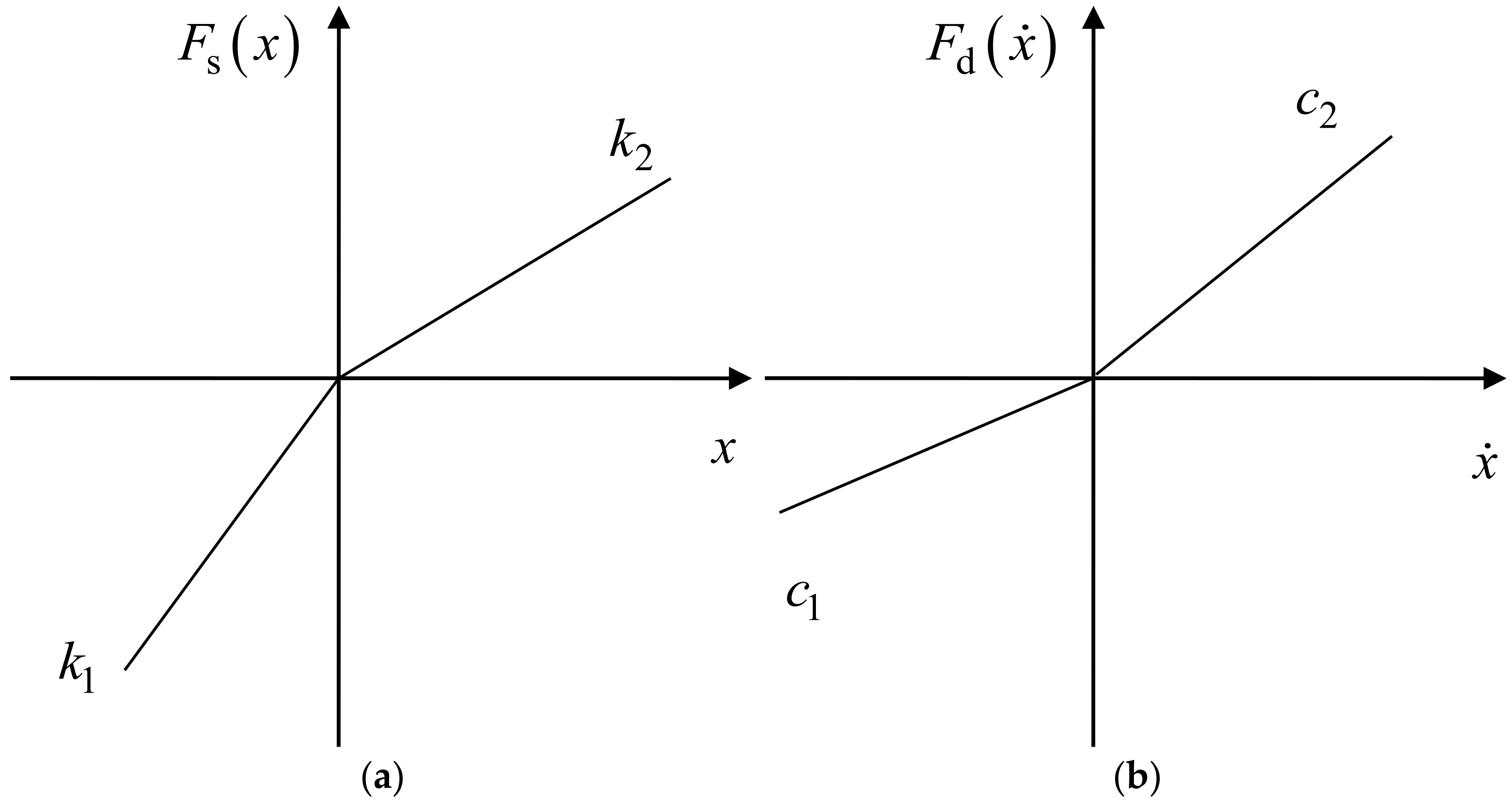
2. Modeling the Asymmetrical Piecewise Characteristics

Figure 1 shows the plots of asymmetrical PWL stiffness in Figure 1a and damping characteristics in Figure 1b, given by

$$F_{\mathrm{s}}\left(x\right)=\left\{\begin{array}{l}{k}_{1}x,\hspace{0.17em}\hspace{0.17em}\hspace{0.17em}\hspace{0.17em}\hspace{0.17em}x\le 0\\ k_{2}x,\hspace{0.17em}\hspace{0.17em}\hspace{0.17em}\hspace{0.17em}\hspace{0.17em}x>0\end{array}\right.\hspace{0.17em}, F_{\mathrm{d}}\left(\dot{x}\right)=\left\{\begin{array}{l}{c}_1\dot{x},\hspace{0.17em}\hspace{0.17em}\hspace{0.17em}\hspace{0.17em}\hspace{0.17em}\dot{x}\le 0\\ c_2\dot{x},\hspace{0.17em}\hspace{0.17em}\hspace{0.17em}\hspace{0.17em}\hspace{0.17em}\dot{x}>0\end{array}\right.\hspace{0.17em}$$

(1)

where $k_1$, $k_2\ge 0$ are the stiffness coefficients and $c_1$, $c_2\ge 0$ are the damping coefficients and $x$ is the travel of vibration isolation system.

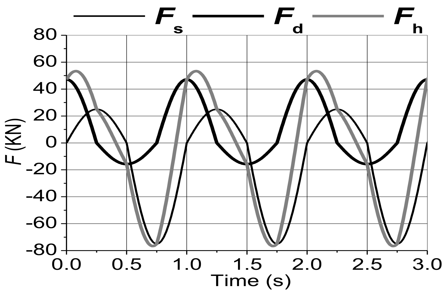
Total hysteretic force developed by vibration isolation system for imposed harmonic motion $x\left(t\right)=X\sin \omega t$, where $\mathrm{\omega }=2\mathrm{\pi }f$, $f$ is the frequency and $X$ is the amplitude, is $F_{\mathrm{h}}\left(x,\dot{x}\right)=F_{\mathrm{s}}\left(x\right)+F_{\mathrm{d}}\left(\dot{x}\right)$. The time histories of hysteretic force $F_{\mathrm{h}}\left(x,\dot{x}\right)$, stiffness force $F_{\mathrm{s}}\left(x\right)$ and damping force $F_{\mathrm{d}}\left(\dot{x}\right)$ are illustrated in Figure 2, for parameters values shown in

Table 1. Values of parameters for hysteretic force.

${\mathit{k}}_{\mathbf{1}}$ [KN/m]	$\hspace{0.17em}{\mathit{k}}_{\mathbf{2}}$ [KN/m]	$\hspace{0.17em}{\mathit{c}}_{\mathbf{1}}$ [KNs/m]	$\hspace{0.17em}{\mathit{c}}_{\mathbf{2}}$ [KNs/m]	$\mathit{X}$ [m]	$\mathit{f}$ [Hz]
1500	500	50	150	0.05	1

.

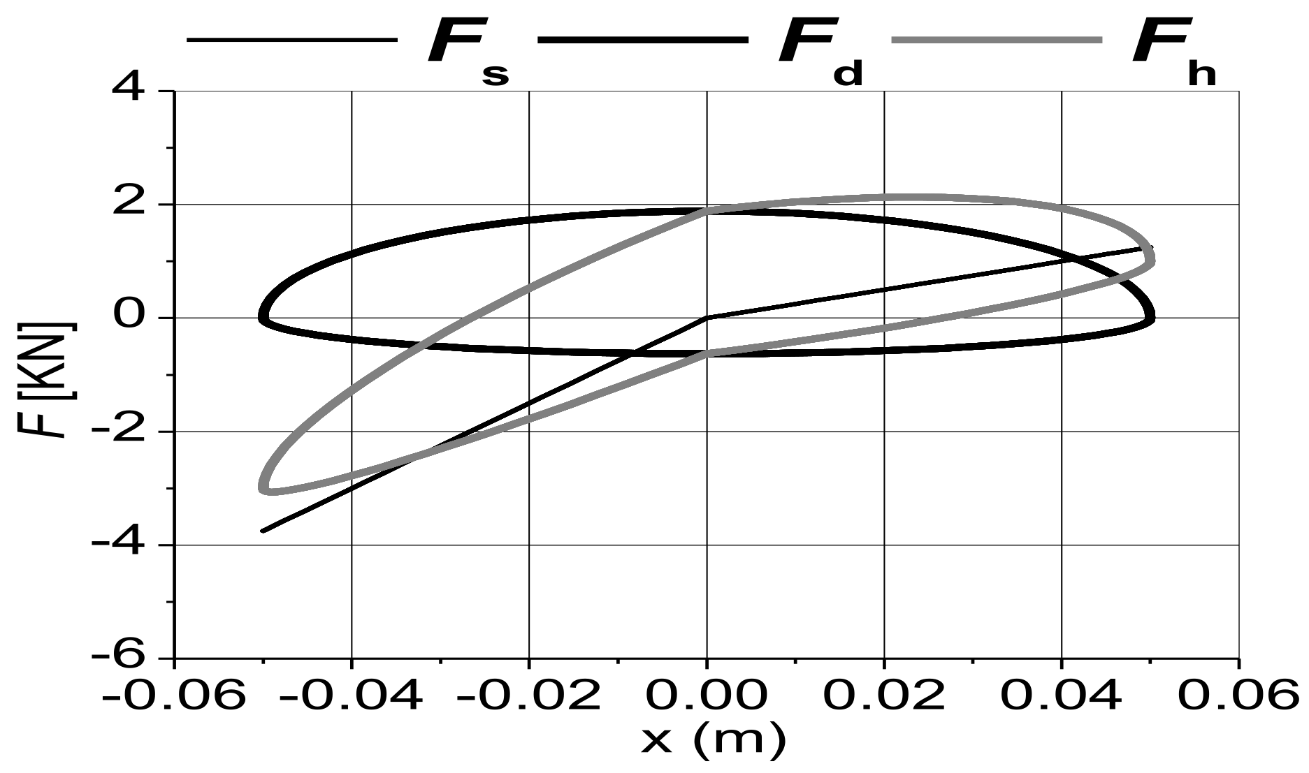
The loops portraying the variation of damping force $F_{\mathrm{d}}$ and total hysteretic force $F_{\mathrm{h}}$ versus the imposed displacement $x$ are shown in Figure 3.

The enclosed area by these loops represents $E_{\mathrm{d}}$, the energy dissipated per cycle:

$$E_{\mathrm{d}}={\displaystyle \underset{0}{\overset{\frac{2\mathrm{\pi }}{\mathrm{\omega }}}{\int }}{F}_{\mathrm{d}}}(\dot{x})\dot{x}\mathrm{d}t=0.5\mathrm{\pi }\mathrm{\omega }{X}^2\left(c_1+c_2\right)$$

(2)

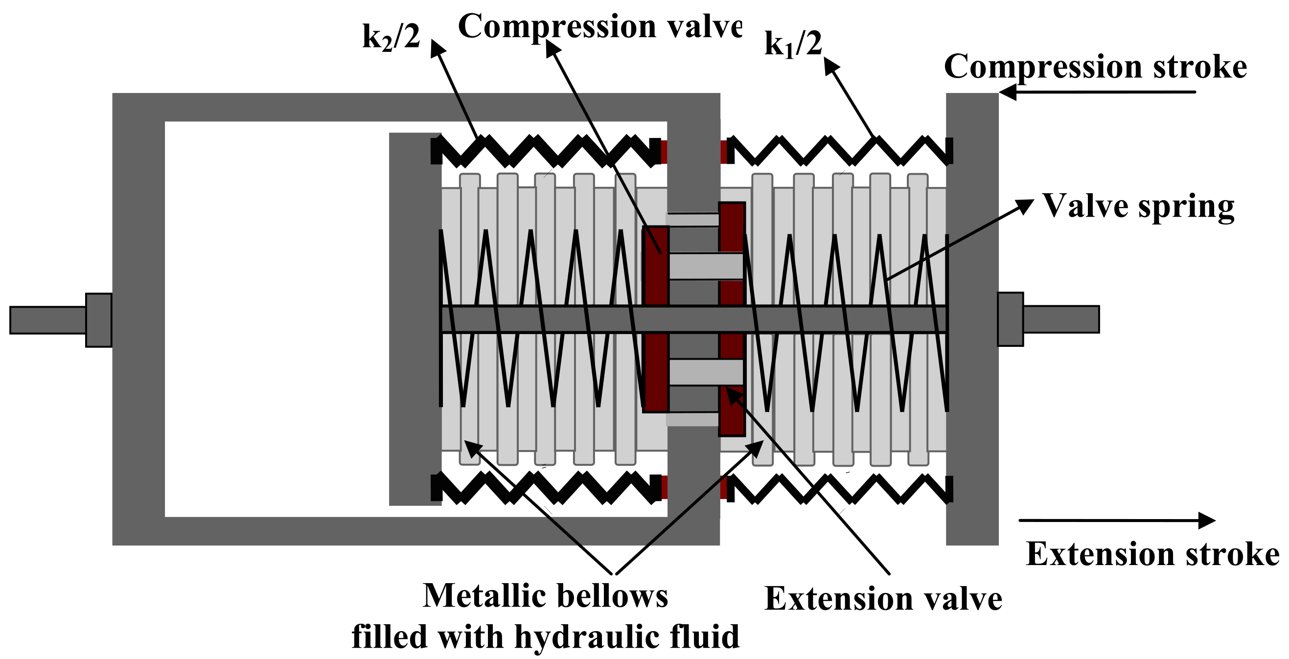
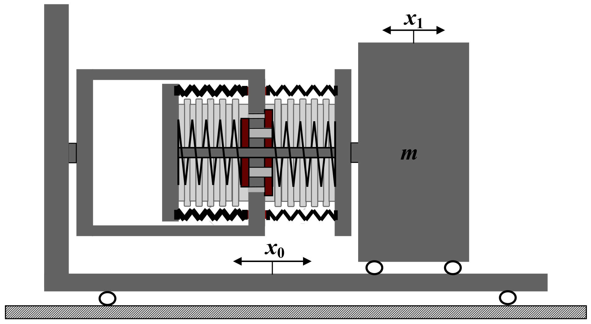
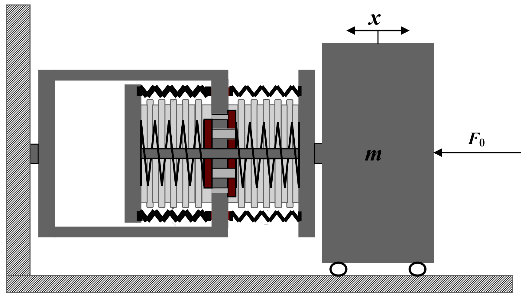
Figure 4 depicts the schematic model of a device with asymmetrical damping and stiffness characteristics.

The metallic bellows, filled with hydraulic fluid, are welded at both ends, and, therefore, the fluid damper is leak proof. The asymmetry of damping force is controlled by the openings of extension and compression valves. The dimensions of valve openings and fluid viscosity must be assessed such that to have laminar flow within the range of damper operating conditions. Since the bellows geometry is identical, there is no need for any volume compensation system. The suspension springs with different stiffness are in the unloaded condition (free length) when the isolation system is in the equilibrium position. Each of them has only one end fixed on the device structure. Therefore, they work only as compression springs for both extension and compression strokes. The bellows longitudinal stiffness, being much smaller than the stiffness of springs, is neglected.

3. Mathematical Model of SDOF Vibration Isolation System with PWL Characteristics

Vibration isolation systems are widely used to reduce the dynamic forces transmitted from the base input to sprung mass (Figure 5) or from the sprung mass to the system base (Figure 6).

The equation of motion for both vibration isolation systems, shown in Figure 5 and Figure 6, can be written as:

$$m\ddot{x}+F_{\mathrm{d}}\left(\dot{x}\right)+F_{\mathrm{s}}\left(x\right)=P_0(t)$$

(3)

where $x=x_1-x_0$ is the relative displacement of sprung mass, $P_0(t)=-m{\ddot{x}}_0$ is the input of system shown in Figure 5, $x_1$ is the absolute displacement and $x_0$ is the base displacement. For the system depicted in Figure 6, $x$ is the absolute displacement of sprung mass, relative to its static equilibrium position, and $P_0(t)=F_0(t)$ is the force applied to the sprung mass. In both cases, $x$ is the stroke (travel) of sprung mass suspension and will be called displacement (disp). The main output of interest for vibration isolation systems are the absolute accelerations of sprung mass ${\ddot{x}}_1$, for system shown in Figure 5, and $\ddot{x}$, for system shown in Figure 6. The absolute acceleration is a measure for mitigation of dynamic forces transmitted through the sprung mass suspension. In the rest of the paper it will be called acceleration and abbreviated as acc. The analytic expressions of asymmetric damping and elastic characteristics $F_{\mathrm{d}}\left(\dot{x}\right)$ and $F_{\mathrm{s}}\left(x\right)$ can be written as

$$\begin{array}{l}{F}_{\mathrm{d}}\left(\dot{x}\right)=0.5\hspace{0.17em}\left[c_1\left(1-\mathrm{sgn}\dot{x}\right)+c_2\left(1+\mathrm{sgn}\dot{x}\right)\right]\dot{x},\hspace{0.17em}\hspace{0.17em}\\ F_{\mathrm{s}}\left(x\right)=0.5\hspace{0.17em}\left[k_1\left(1-\mathrm{sgn}x\right)+k_2\left(1+\mathrm{sgn}x\right)\right]x.\end{array}$$

(4)

Introducing the notations

$$\begin{array}{l}\hspace{0.17em}{\mathrm{\omega }}_1=2\mathrm{\pi }{f}_1=\sqrt{\frac{k_1}{m}},\hspace{0.17em}\hspace{0.17em}{\mathrm{\omega }}_2=2\mathrm{\pi }{f}_2=\sqrt{\frac{k_2}{m}},\hspace{0.17em}{\zeta }_1=\frac{c_1}{2{\mathrm{\omega }}_{1}m},\hspace{0.17em}\hspace{0.17em}{\zeta }_2=\frac{c_2}{2{\mathrm{\omega }}_{2}m}\\ \hspace{0.17em}\mathrm{\beta }=\frac{c_2}{c_1}=\frac{{\zeta }_2{f}_2}{{\zeta }_1{f}_1},\hspace{0.17em}\gamma =\sqrt{\frac{k_2}{k_1}}=\frac{f_2}{f_1}\\ \hspace{0.17em}\hspace{0.17em}\hspace{0.17em}{f}_{\mathrm{d}}\left(\dot{x}\right)=\hspace{0.17em}\frac{F_{\mathrm{d}}\left(\dot{x}\right)}{m}\hspace{0.17em},\hspace{0.17em}\hspace{0.17em}\hspace{0.17em}{f}_{\mathrm{s}}\left(x\right)=\hspace{0.17em}\frac{F_{\mathrm{s}}\left(x\right)}{m}\hspace{0.17em}\hspace{0.17em}\hspace{0.17em}\mathrm{and}\hspace{0.17em}\hspace{0.17em}{p}_0\left(t\right)\hspace{0.17em}=\hspace{0.17em}\frac{P_0\left(t\right)}{m},\end{array}$$

(5)

the equation of motion (3) becomes

$$\ddot{x}+f_{\mathrm{d}}\left(\dot{x}\right)+f_{\mathrm{s}}\left(x\right)=p_0\left(t\right)$$

(6)

where

$$\begin{array}{l}{f}_{\mathrm{d}}\left(\dot{x}\right)={\zeta }_1{\mathrm{\omega }}_1\hspace{0.17em}\left[\left(\mathrm{\beta }+1\right)\dot{x}+\left(\mathrm{\beta }-1\right)\left|\dot{x}\right|\hspace{0.17em}\right],\hspace{0.17em}\hspace{0.17em}\\ f_{\mathrm{s}}\left(x\right)=0.5{\mathrm{\omega }}_1^2\left[\left({\gamma }^2+1\right)x+\left({\gamma }^2-1\right)\left|x\right|\hspace{0.17em}\right].\end{array}$$

(7)

From (2) and (5), one can see that asymmetry parameter $\mathrm{\beta }$ is the ratio of dissipated energy per rebound $\left(E_{\mathrm{d}2}=0.5\mathrm{\pi }\mathrm{\omega }{X}^2{c}_2\right)$ and bound $\left(E_{\mathrm{d}1}=0.5\mathrm{\pi }\mathrm{\omega }{X}^2{c}_1\right)$ strokes for an imposed harmonic motion.

4. The Effect of Asymmetry of Damping and Restoring Characteristics on the Dynamic Behavior of Piecewise Linear Systems under Stationary Random Excitation

In general, the asymmetry of damping or stiffness characteristics leads to a drift of sprung mass average position in dynamic regime, different from its static equilibrium position. Nevertheless, by a suitable combination of the asymmetry parameters $\mathrm{\beta }$ and $\gamma$, one can obtain outputs of PWL systems with almost no drift.

Suppose that $p_0\left(t\right)$ is a stationary Gaussian random process with zero mean and standard deviation ${\mathrm{\sigma }}_0$. If $x\left(t\right)$ is the steady state stationary solution of Equation (6), with constant mean value $\hspace{0.17em}{m}_{\mathrm{x}}=\mathrm{E}\left[x\right]$ then $\hspace{0.17em}\mathrm{E}\left[\dot{x}\right]\hspace{0.17em}=\mathrm{E}\left[\ddot{x}\right]\hspace{0.17em}=0$. Therefore, by applying the average operator corresponding to joint distribution of the output of Equation (6), $m_{\mathrm{x}}$ is obtained as follows:

$$m_{\mathrm{x}}=-\frac{m_{\left|\mathrm{x}\right|}}{{\gamma }^2+1}\left[\left({\gamma }^2-1\right)+2\left(\mathrm{\beta }-1\right){\zeta }_1\frac{m_{\left| \dot{\mathrm{x}}\right|}}{{\mathrm{\omega }}_1{m}_{\left|\mathrm{x}\right|}}\right]$$

(8)

where

$$\hspace{0.17em}{m}_{\left|\mathrm{x}\right|}=\hspace{0.17em}\mathrm{E}\left[\left|x\right|\right]\hspace{0.17em} \mathrm{and} m_{\left| \dot{\mathrm{x}}\right|}=\mathrm{E}\left[\left|\dot{x}\right|\right]$$

(9)

The relation (8) shows that $m_{\mathrm{x}}=0$ if $\gamma =1,\hspace{0.17em}\mathrm{\beta }=1$; $m_{\mathrm{x}}<0$ if $\gamma >1,\hspace{0.17em}\mathrm{\beta }>1$ and $m_{\mathrm{x}}>0$ if $\gamma <1,\hspace{0.17em}\mathrm{\beta }<1$. It is worth noting that by assuming $m_{\left| \dot{\mathrm{x}}\right|}/{\mathrm{\omega }}_1{m}_{\left|\mathrm{x}\right|}\approx 1$, for all case studies considered in this work (including $\gamma >1,\hspace{0.17em}\hspace{0.17em}\mathrm{\beta }<1$ or $\gamma <1,\hspace{0.17em}\mathrm{\beta }>1$), the sign of $m_{\mathrm{x}}$ could be predicted by determining the sign of expression $\hspace{0.17em}S\left(\gamma ,\mathrm{\beta },{\zeta }_1\right)=-\left[\left({\gamma }^2-1\right)+2\left(\mathrm{\beta }-1\right){\zeta }_1\right]$, without being necessary the numerical simulation values from (9).

5. Gaussian Equivalent Linearization Method of PWL Systems

The Gaussian equivalent linear system (LinEq) of system (6), where $p_0\left(t\right)$ is a stationary Gaussian process,$\hspace{0.17em}\mathrm{E}\left[p_0\left(t\right)\right]=0$ and $\mathrm{E}\left[p_0^2\left(t\right)\right]={\mathrm{\sigma }}_0^2$ is written as

$$\ddot{x}+2{\zeta }_{\mathrm{e}}{\mathrm{\omega }}_{\mathrm{e}}\dot{x}+{\mathrm{\omega }}_{\mathrm{e}}^{2}x=p_0\left(t\right)$$

(10)

The joint probability density function of the Gaussian stationary solution of equivalent linear system is

$$\begin{array}{c}g\left(x,\dot{x}\right)=g_1\left(x\right)g_2\left(\dot{x}\right)\\ g_1\left(x\right)=\frac{1}{\sqrt{2\mathrm{\pi }}{\mathrm{\sigma }}_{\mathrm{x}}}\exp \left[-\frac{x^2}{2{\mathrm{\sigma }}_{\mathrm{x}}^2}\right]\hspace{0.17em}\hspace{0.17em},\hspace{0.17em}{g}_2\left(\dot{x}\right)=\frac{1}{\sqrt{2\mathrm{\pi }}{\mathrm{\sigma }}_{ \dot{\mathrm{x}}}}\exp \left[-\frac{{\dot{x}}^2}{2{\mathrm{\sigma }}_{ \dot{\mathrm{x}}}^2}\right]\hspace{0.17em},\end{array}$$

(11)

where ${\mathrm{\sigma }}_{\mathrm{x}}={\mathrm{\sigma }}_{\mathrm{x}}\left({\mathrm{\omega }}_{\mathrm{e}},\hspace{0.17em}{\zeta }_{\mathrm{e}}\right)$ and ${\mathrm{\sigma }}_{ \dot{\mathrm{x}}}={\mathrm{\sigma }}_{ \dot{\mathrm{x}}}\left({\mathrm{\omega }}_{\mathrm{e}},\hspace{0.17em}{\zeta }_{\mathrm{e}}\right)$ are the standard deviations for the solution of Equation (10).

The variance of the acceleration ${\ddot{x}}_1=2{\zeta }_{\mathrm{e}}{\mathrm{\omega }}_{\mathrm{e}}\dot{x}+{\mathrm{\omega }}_{\mathrm{e}}^{2}x$ of the equivalent linear system is

$${\mathrm{\sigma }}_{{ \ddot{\mathrm{x}}}_1}^2=E\left[{\ddot{x}}_1^2\right]=4{\zeta }_{\mathrm{e}}^2{\mathrm{\omega }}_{\mathrm{e}}^{2}E\left[{\dot{x}}^2\right]+{\mathrm{\omega }}_{\mathrm{e}}^{4}E\left[x^2\right]={\mathrm{\omega }}_{\mathrm{e}}^2\left[4{\zeta }_{\mathrm{e}}^2{\mathrm{\sigma }}_{ \dot{\mathrm{x}}}^2+{\mathrm{\omega }}_{\mathrm{e}}^2{\mathrm{\sigma }}_{\mathrm{x}}^2\right]$$

(12)

Applying the linearization criteria,

$$\begin{array}{l}{\epsilon }_{\mathrm{e}}\left({\mathrm{\omega }}_{\mathrm{e}}\right)=E\left[{\left(f_{\mathrm{s}}\left(x\right)-{\mathrm{\omega }}_{\mathrm{e}}^{2}x\right)}^2\right]=\min ,\hspace{0.17em}\hspace{0.17em}\hspace{0.17em}\hspace{0.17em}\hspace{0.17em}\hspace{0.17em}\hspace{0.17em}\hspace{0.17em}\hspace{0.17em}\hspace{0.17em}\hspace{0.17em}\hspace{0.17em}\frac{\partial {\epsilon }_{\mathrm{e}}\left({\mathrm{\omega }}_{\mathrm{e}}\right)}{\partial {\mathrm{\omega }}_{\mathrm{e}}}=0\\ {\epsilon }_{\mathrm{d}}\left({\zeta }_{\mathrm{e}},{\mathrm{\omega }}_{\mathrm{e}}\right)=E\left[{\left(f_{\mathrm{d}}\left(\dot{x}\right)-2{\zeta }_{\mathrm{e}}{\mathrm{\omega }}_{\mathrm{e}}\dot{x}\right)}^2\right]=\min \hspace{0.17em},\hspace{0.17em}\hspace{0.17em}\frac{\partial {\epsilon }_{\mathrm{d}}\left({\zeta }_{\mathrm{e}},{\mathrm{\omega }}_{\mathrm{e}}\right)}{\partial {\zeta }_{\mathrm{e}}}=0\end{array}$$

(13)

the linear equivalent stiffness and damping coefficients are obtained using (6), (11) and (13):

$$\begin{array}{l}{\mathrm{\omega }}_{\mathrm{e}}^2=\frac{E\left[x{f}_{\mathrm{s}}\left(x\right)\right]}{E\left[x^2\right]}=\hspace{0.17em}\frac{{\mathrm{\omega }}_1^2+{\mathrm{\omega }}_2^2}{2}=\frac{{\mathrm{\omega }}_1^2\left(1+{\gamma }^2\right)}{2},\\ {\zeta }_{\mathrm{e}}=\frac{E\left[\dot{x}{f}_{\mathrm{d}}\left(\dot{x}\right)\right]}{2{\mathrm{\omega }}_{\mathrm{e}}E\left[{\dot{x}}^2\right]}=\frac{{\zeta }_1{\mathrm{\omega }}_1+{\zeta }_2{\mathrm{\omega }}_2}{2{\mathrm{\omega }}_{\mathrm{e}}}=\frac{{\zeta }_1{\mathrm{\omega }}_1\left(1+\mathrm{\beta }\right)}{2{\mathrm{\omega }}_{\mathrm{e}}}\hspace{0.17em}.\end{array}$$

(14)

Using (14) one can write

$$f_{\mathrm{e}}=f_1\sqrt{\frac{1+{\gamma }^2}{2}},\hspace{0.17em}\hspace{0.17em}\hspace{0.17em}{\zeta }_{\mathrm{e}}=\frac{{\zeta }_1\left(1+\mathrm{\beta }\right)}{\sqrt{2\left(1+{\gamma }^2\right)}},\hspace{0.17em}\hspace{0.17em}{f}_{\mathrm{e}}={\mathrm{\omega }}_{\mathrm{e}}/2\mathrm{\pi },\hspace{0.17em}\hspace{0.17em}{f}_1={\mathrm{\omega }}_1/2\mathrm{\pi }$$

(15)

In order to highlight the advantage of using the vibration isolation systems with asymmetric PWL characteristics, the obtained results are compared with those of optimal linear equivalent system.

For given values of linear equivalent system ${\zeta }_{\mathrm{e}},\hspace{0.17em}{f}_{\mathrm{e}}$ and chosen values of asymmetry parameters $\gamma ,\hspace{0.17em}\mathrm{\beta }$, relations (15) yield:

$$f_1=f_{\mathrm{e}}\sqrt{\frac{2}{1+{\gamma }^2}}\hspace{0.17em},\hspace{0.17em}\hspace{0.17em}{f}_2=\gamma f_1,\hspace{0.17em}\hspace{0.17em}{\zeta }_1=\frac{{\zeta }_{\mathrm{e}}\sqrt{2\left(1+{\gamma }^2\right)}}{1+\mathrm{\beta }} \mathrm{and} {\zeta }_2=\frac{\mathrm{\beta }}{\gamma }{\zeta }_1$$

(16)

From (16) one can obtain the balance equation between the energy dissipated by PWL asymmetric system and its linear equivalent system per cycle for same imposed harmonic motion:

$$\hspace{0.17em}{\zeta }_1{f}_1+{\zeta }_2{f}_2=2f_{\mathrm{e}}{\zeta }_{\mathrm{e}}$$

(17)

As one can see from previous relations, there are an infinite number of PWL asymmetric systems having same linear equivalent system.

Following [27], the standard deviation of the stationary steady state acceleration of sprung mass for stochastic linear system (10) with Gaussian white noise excitation $p_0\left(t\right)$ and constant spectral density $S_0$ is

$${\mathrm{\sigma }}_{{ \ddot{\mathrm{x}}}_1\mathrm{e}}=\sqrt{2S_0{\displaystyle \underset{0}{\overset{\infty }{\int }}{A}_{{ \ddot{\mathrm{x}}}_1\mathrm{e}}^2\left(\mathrm{\omega }\right)} \mathrm{d}\mathrm{\omega }}=\sqrt{\frac{\mathrm{\pi }{\mathrm{\omega }}_{\mathrm{e}}{S}_0\left(1+4{\zeta }_{\mathrm{e}}^2\right)}{2{\zeta }_{\mathrm{e}}}},$$

(18)

where $A_{{ \ddot{\mathrm{x}}}_1\mathrm{e}}\left(\mathrm{\omega }\right)$ is the acceleration transmissibility factor of linear equivalent system:

$$\hspace{0.17em}\hspace{0.17em}\hspace{0.17em}\hspace{0.17em}\hspace{0.17em}\hspace{0.17em}\hspace{0.17em}\hspace{0.17em}\hspace{0.17em}\hspace{0.17em}\hspace{0.17em}\hspace{0.17em}\hspace{0.17em}\hspace{0.17em}\hspace{0.17em}{A}_{{ \ddot{\mathrm{x}}}_1\mathrm{e}}\left(\mathrm{\omega }\right)\hspace{0.17em}\hspace{0.17em}=\sqrt{\frac{4{\zeta }_{\mathrm{e}}^2{\mathrm{\omega }}_{\mathrm{e}}^2{\mathrm{\omega }}^2+{\mathrm{\omega }}_{\mathrm{e}}^4}{{\mathrm{\omega }}^4+2(2{\zeta }_{\mathrm{e}}^2-1){\mathrm{\omega }}_{\mathrm{e}}^2{\mathrm{\omega }}^2+{\mathrm{\omega }}_{\mathrm{e}}^4}}$$

(19)

The optimum value of damping ratio ${\zeta }_{\mathrm{e}}$, which minimizes the std value of sprung mass acceleration is ${\zeta }_{\mathrm{e}}=0.5$, and its minimum value is ${\mathrm{\sigma }}_{{ \ddot{\mathrm{x}}}_1\min }=\sqrt{2\mathrm{\pi }{\mathrm{\omega }}_{\mathrm{e}}{S}_0}$. Taking $S_0=1\hspace{0.17em}{\mathrm{m}}^2{\mathrm{s}}^{-3}$ and ${\mathrm{\omega }}_{\mathrm{e}}=2\mathrm{\pi }\hspace{0.17em}\mathrm{rad}/\mathrm{s}$, the optimum std value of acceleration is ${\mathrm{\sigma }}_{{\ddot{\mathrm{x}}}_1\min }\cong 6.28\hspace{0.17em}{\mathrm{ms}}^{-2}$. For numerical integration, the input is a limited bandwidth white noise, and std value of acceleration is calculated as

$${\mathrm{\sigma }}_{{ \ddot{\mathrm{x}}}_1\mathrm{e}}\cong \sqrt{2{\displaystyle \underset{{\mathrm{\omega }}_{\min }}{\overset{{\mathrm{\omega }}_{\max }}{\int }}{A}_{{ \ddot{\mathrm{x}}}_1\mathrm{e}}^2\left(\mathrm{\omega }\hspace{0.17em};{\zeta }_{\mathrm{e}},\hspace{0.17em}{\mathrm{\omega }}_{\mathrm{e}}\right)\hspace{0.17em}}\mathrm{d}\mathrm{\omega }}\cong 6.21\hspace{0.17em}{\mathrm{ms}}^{-2},$$

(20)

where $\hspace{0.17em}\hspace{0.17em}0.2\le \mathrm{\omega }\le 128\hspace{0.17em}$ and $\mathrm{\omega }$ is measured in rad/s, which is a good approximation of optimum value ${\mathrm{\sigma }}_{{ \ddot{\mathrm{x}}}_1\min }$, calculated over the whole range of angular frequency $\left[0,\hspace{0.17em}\infty \right)$. The results obtained by the proposed approach will be compared with those obtained by the Gaussian equivalent linearization method.

6. The Response of PWL Systems to Stationary Gaussian Random Input with Rational Spectral Density (Shape Filtered White Noise)

According to [28], the covariance function and spectral density of stationary Gaussian random input $p_0(t)$ are

$$\begin{array}{l}{C}_0\left(\mathrm{\tau }\right)={\mathrm{\sigma }}_0^2{\mathrm{e}}^{-a\left|\mathrm{\tau }\right|}\cos b\mathrm{\tau },\hspace{0.17em}\hspace{0.17em}a>0,\hspace{0.17em}\hspace{0.17em}b\ge 0,\hspace{0.17em}\hspace{0.17em}\hspace{0.17em}\hspace{0.17em}\\ S_0\left(\mathrm{\omega }\right)=\frac{{\mathrm{\sigma }}_0^2}{\mathrm{\pi }}\hspace{0.17em}\frac{a\left({\mathrm{\omega }}^2+a^2+b^2\right)}{{\mathrm{\omega }}^4+2\left(a^2-b^2\right){\mathrm{\omega }}^2+{\left(a^2+b^2\right)}^2}\hspace{0.17em},\end{array}$$

(21)

where ${\mathrm{\sigma }}_0^2=\hspace{0.17em}{\displaystyle \underset{-\infty }{\overset{\infty }{\int }}{S}_0\left(\mathrm{\omega }\right)\mathrm{d}\mathrm{\omega }}=\hspace{0.17em}2{\displaystyle \underset{0}{\overset{\infty }{\int }}{S}_0\left(\mathrm{\omega }\right)\mathrm{d}\mathrm{\omega }}\hspace{0.17em}.$ The above expression of $S_0\left(\mathrm{\omega }\right)$ can be viewed as the spectral density of the Gaussian stationary random process $p_0(t)$, obtained as the output of a second order shape filter to a stationary Gaussian white noise process $z\left(t\right)$ with $\hspace{0.17em}\mathrm{E}\left[z\left(t\right)\right]=0,\hspace{0.17em}\hspace{0.17em}\mathrm{E}\left[z\left(t\right)z\left(t+\mathrm{\tau }\right)\right]=2\pi S_0\delta \left(\mathrm{\tau }\right)$, where $\delta \left(\mathrm{\tau }\right)$ is the Dirac delta function. In order to determine the equations of the second order shape filter, the spectral density (21) is written under the form

$$S_0\left(\omega \right)=\frac{{\left|P\left(\mathrm{i}\omega \right)\right|}^2}{{\left|Q\left(\mathrm{i}\omega \right)\right|}^2}=\frac{{\left|b_0(\mathrm{i}\mathrm{\omega })+b_1\right|}^2}{{\left|a_0{(\mathrm{i}\mathrm{\omega })}^2+a_1(\mathrm{i}\mathrm{\omega })+a_2\right|}^2}\hspace{0.17em},$$

(22)

where $\hspace{0.17em}{b}_0={\mathrm{\sigma }}_0\sqrt{\frac{a}{\mathrm{\pi }}},\hspace{0.17em}\hspace{0.17em}\hspace{0.17em}{b}_1={\mathrm{\sigma }}_0\sqrt{\frac{a(a^2+b^2)}{\mathrm{\pi }}},\hspace{0.17em}\hspace{0.17em}{a}_0=1,\hspace{0.17em}\hspace{0.17em}{a}_1=2a,\hspace{0.17em}\hspace{0.17em}{a}_2=a^2+b^2$.

The output $u_1\left(t\right)$ of the following first order differential system with the white noise excitation $z\left(t\right)$ is a Gaussian stationary random process with spectral density $S_0\left(\mathrm{\omega }\right)$:

$$\dot{u}=Au+gz,\hspace{0.17em}\hspace{0.17em}$$

(23)

where

$$\begin{array}{c}\hspace{0.17em}A=\left[\begin{array}{cc}0& 1\\ -a_2& -a_1\end{array}\right],\hspace{0.17em}\hspace{0.17em}u=\left[\begin{array}{c}{u}_1\\ u_2\end{array}\right],\hspace{0.17em}\hspace{0.17em}g=\left[\begin{array}{c}{g}_1\\ g_2\end{array}\right]\\ g_1={\mathrm{\sigma }}_0\sqrt{\frac{a}{\mathrm{\pi }}},\hspace{0.17em}\hspace{0.17em}{g}_2={\mathrm{\sigma }}_0\sqrt{\frac{a}{\mathrm{\pi }}}\left(\sqrt{a^2+b^2}-2a\hspace{0.17em}\right) \mathrm{and} p_0\left(t\right)=u_1\left(t\right).\end{array}$$

(24)

In order to study the behavior of asymmetric PWL systems excited by stationary random input with rational spectral density, a linear system of first order stochastic equations is assessed such as the first component of its solution vector has the same transmissibility factor as the chosen output of the considered piecewise linear system [23]. The statistical parameters of obtained stochastic differential equations are determined by solving the associated Lyapunov equation.

Since the mean value of PWL acceleration response system has zero mean, the transmissibility factors corresponding to standard deviation and root mean square values are identical.

The discrete values of transmissibility factor corresponding to standard deviation of acceleration ${\ddot{x}}_1\left(t\right)$ is defined as:

$$\hspace{0.17em}\hspace{0.17em}\hspace{0.17em}\hspace{0.17em}\hspace{0.17em}{\tilde{A}}_{{ \ddot{\mathrm{x}}}_1}\left({\mathrm{\omega }}_i\right)=\hspace{0.17em}\frac{{\mathrm{\sigma }}_{{\ddot{x}}_1}\left({\mathrm{\omega }}_i\right)}{{\mathrm{\sigma }}_{p_{0i}}}=\frac{\sqrt{2}\hspace{0.17em}{\mathrm{\sigma }}_{{\ddot{x}}_1}\left({\mathrm{\omega }}_i\right)}{P_0},\hspace{0.17em}\hspace{0.17em}i=\overline{1,N}$$

(25)

These values are obtained by numerical integration of Equation (6), using Matlab Simulink, for harmonic inputs with constant amplitude and different frequencies in the twelfth octave band:

$$p_0{}_i\left(t\right)=P_0\sin {\mathrm{\omega }}_{i}t,\hspace{0.17em}\hspace{0.17em}\hspace{0.17em}{\mathrm{\omega }}_i=2\mathrm{\pi }\hspace{0.17em}{f}_i,\hspace{0.17em}\hspace{0.17em}{f}_1=0.3\mathrm{Hz},\hspace{0.17em}{f}_N=20.05\mathrm{Hz}, \hspace{0.17em}\hspace{0.17em}{f}_i=2^{\frac{i-1}{12}}{f}_1,\hspace{0.17em}\hspace{0.17em}\hspace{0.17em}i=\overline{1,N}$$

(26)

where $P_0=1 \mathrm{m}/{\mathrm{s}}^2$, $N=\left[\frac{\log \left(f_N/f_1\right)}{\log \left(f_2/f_1\right)}\right]+2=114$.

It should be mentioned that the transmissibility factors of PWL systems, with asymmetry type (affine) [29], considered in this paper, do not depend on the amplitude $P_0$ of the applied harmonic input with variable frequency, as long as they are computed for the stationary regime. The numerical values ${\tilde{A}}_{{ \ddot{\mathrm{x}}}_1}\left({\mathrm{\omega }}_i\right),\hspace{0.17em}i=\overline{1,N}$, can be fitted using the Least Squares Method, by analytical expressions having the form

$$A_{{ \ddot{\mathrm{x}}}_1}\left(\mathrm{\omega }\right)\hspace{0.17em}\hspace{0.17em}=\sqrt{\frac{P_1{\mathrm{\omega }}^2+P_2}{{\mathrm{\omega }}^4+Q_1{\mathrm{\omega }}^2+Q_2}}.$$

(27)

The transmissibility factor $A_{{ \ddot{\mathrm{x}}}_1}\left(\mathrm{\omega }\right)$ is written as:

$$A_{{ \ddot{\mathrm{x}}}_1}\left(\mathrm{\omega }\right)\hspace{0.17em}\hspace{0.17em}=\left|\frac{b_0\left(\mathrm{i}\mathrm{\omega }\right)+b_1}{{\left(\mathrm{i}\mathrm{\omega }\right)}^2+a_1\left(\mathrm{i}\mathrm{\omega }\right)+a_2}\right|=\sqrt{\frac{b_0^2{\mathrm{\omega }}^2+b_1^2}{{\mathrm{\omega }}^4+\left(a_1^2-2a_2\right){\mathrm{\omega }}^2+a_2^2}}$$

(28)

From relations (27) and (28), the following nonlinear algebraic systems of equations for unknown coefficients $b_0,b_1,a_1,\hspace{0.17em}{a}_2$, are obtained

$$\left\{\begin{array}{l}{b}_0^2=P_1\\ b_1^2=P_2\end{array}\right.,\hspace{0.17em}\hspace{0.17em}\hspace{0.17em}\left\{\begin{array}{l}{a}_1^2-2a_2=Q_1\\ a_2^2=\hspace{0.17em}{Q}_2\end{array}\right.$$

(29)

The attached linear system corresponding to transmissibility factor (28) can be written as

$$\hspace{0.17em}\hspace{0.17em}\hspace{0.17em}\dot{u}=Au+c{p}_0\hspace{0.17em},$$

(30)

where

$$A=\hspace{0.17em}\hspace{0.17em}\hspace{0.17em}\left[\hspace{0.17em}\begin{array}{cc}0& 1\\ -a_2& -a_1\end{array}\right]\hspace{0.17em},\hspace{0.17em}\hspace{0.17em}u=\left[\begin{array}{c}{u}_1\\ u_2\end{array}\right]\hspace{0.17em}\hspace{0.17em},\hspace{0.17em}\hspace{0.17em}c=\left[\begin{array}{c}{c}_1\\ c_2\end{array}\right],\hspace{0.17em}\hspace{0.17em}\hspace{0.17em}\left\{\begin{array}{l}{c}_1=b_0\\ c_2=b_1-a_1{c}_1\end{array}\right.$$

(31)

The transmissibility factor $A_{{ \ddot{\mathrm{x}}}_1}\left(\mathrm{\omega }\right)\hspace{0.17em}\cong A_{{\mathrm{\sigma }}_{u_1}}\left(\mathrm{\omega }\right)=\sqrt{2}{\mathrm{\sigma }}_{u_1}/P_0$, where $u_1$ is the first component of the solution vector $u$. The system (30) is asymptotically stable if $a_1, a_2>0$. Therefore, from the sets of real solutions of (29), one must select only the solutions that fulfill these conditions.

In what follows, the study is carried out for several asymmetric PWL systems for which the stochastic equivalent linear system is the optimal one. The parameters of PWL systems, given in

Table 2. The parameters of PWL systems.

Case	$\mathit{\zeta }{\hspace{0.17em}}_1$	${\mathit{f}}_1\hspace{0.17em}[\mathbf{Hz}]$	$\mathit{\gamma }$	$\mathit{\beta }$	$\mathit{\zeta }{\hspace{0.17em}}_2$	${\mathit{f}}_2\hspace{0.17em}[\mathbf{Hz}]$
1	0.05	0.25	5.57	79	0.71	1.39
2	0.1	0.5	2.65	19	0.72	1.33
3	0.1	0.7	1.76	13.31	0.76	1.23
4	0.2	0.4	3.39	11.5	0.68	1.36
5	0.3	0.6	2.13	4.55	0.64	1.28
6	0.7	1.1	0.81	0.3	0.26	0.89

, were obtained by using relations (16).

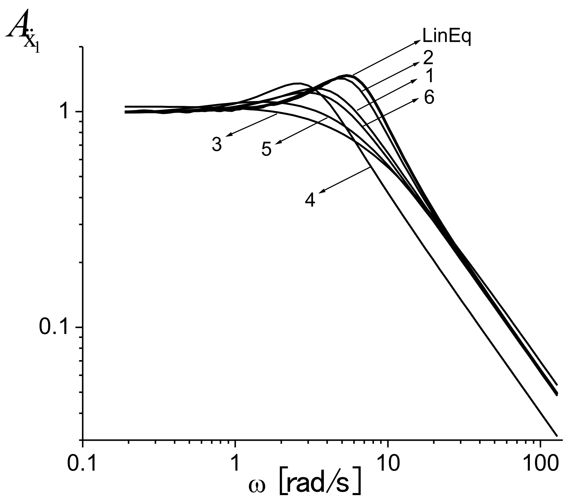
In Figure 7, the transmissibility factor ${\tilde{A}}_{{ \ddot{\mathrm{x}}}_1}\left({\mathrm{\omega }}_i\right)$ obtained by numerical integration for the asymmetric PWL systems from Table 2 is compared with transmissibility factor of their stochastic equivalent linear system ($\zeta {\hspace{0.17em}}_1={\zeta }_2=0.5$, $\gamma =\mathrm{\beta }=1$, $f_1\hspace{0.17em}=f_2=1$ Hz).

Table 3. The transmissibility factors of asymmetric PWL systems.

Case	${\mathit{\zeta }}_1$	${\mathit{f}}_1 \left[\mathbf{Hz}\right]$	${\mathit{\zeta }}_2$	${\mathit{f}}_2 \left[\mathbf{Hz}\right]$	${\mathit{\sigma }}_{{\ddot{\mathbf{x}}}_1} [\mathbf{m}/{\mathbf{s}}^2]$
1	0.05	0.25	0.71	1.39	4.52
2	0.1	0.5	0.72	1.33	4.98
3	0.1	0.7	0.76	1.23	5.35
4	0.2	0.4	0.68	1.36	4.71
5	0.3	0.6	0.64	1.28	5.12
6	0.7	1.1	0.26	0.89	5.97

presents the standard deviation values of the acceleration obtained by using a similar relation to (20), for the transmissibility factors of asymmetric PWL systems shown in Figure 7.

The above results show that the piecewise linear systems with asymmetrical damping and stiffness characteristics can provide a better vibration isolation (lower force transmissibility) than the optimum equivalent linear system (${\mathrm{\sigma }}_{{ \ddot{\mathrm{x}}}_1}=6.21$ [m/s²]).

7. Attached Linear System for Different Outputs of PWL Systems Excited by a Second Order Shape Filtered White Noise

In order to estimate the statistical characteristics for the output of asymmetric PWL systems, the corresponding attached linear systems will be determined in the next sections. The stochastic equations of attached linear system for the piecewise linear system (6), with shape filtered white noise excitation, is obtained by combining Equations (23) and (30):

$$\dot{u}=Au+gz,$$

(32)

where

$$\begin{array}{c}A=\hspace{0.17em}\hspace{0.17em}\hspace{0.17em}\left[\hspace{0.17em}\begin{array}{cccc}0& 1& c_1& 0\\ -a_2& -a_1& c_2& 0\\ 0& 0& 0& 1\\ 0& 0& -a_4& -a_3\end{array}\right]\hspace{0.17em},\hspace{0.17em}\hspace{0.17em}u=\left[\begin{array}{c}{u}_1\\ u_2\\ u_3\\ u_4\end{array}\right]\hspace{0.17em}\hspace{0.17em},\hspace{0.17em}\hspace{0.17em}g=\left[\begin{array}{c}0\\ 0\\ g_1\\ g_2\end{array}\right]\\ u_1\left(t\right)={\ddot{x}}_1\left(t\right),\hspace{0.17em}\hspace{0.17em}{u}_3\left(t\right)=p_0\left(t\right)\\ \hspace{0.17em}{a}_3=2a,\hspace{0.17em}\hspace{0.17em}{a}_4=a^2+b^2,g_1={\mathrm{\sigma }}_0\sqrt{\frac{a}{\mathrm{\pi }}},\hspace{0.17em}\hspace{0.17em}{g}_2={\mathrm{\sigma }}_0\sqrt{\frac{a}{\mathrm{\pi }}}\left(\sqrt{a^2+b^2}-2a\hspace{0.17em}\right)\end{array}$$

(33)

The covariance matrix $C=\left(c_{ij}\right),\hspace{0.17em}\hspace{0.17em}{c}_{ij}=c_{ji}=\underset{t\to \infty }{\lim }\mathrm{E}\left[u_i\left(t\right)u_j\left(t\right)\right],\hspace{0.17em}\hspace{0.17em}i,j=\overline{1,4}$ of the steady state stationary solution of stochastic linear system (32) satisfies [30] the Lyapunov Equation:

$$AC+C{A}^{\mathrm{T}}+2\mathrm{\pi }{S}_{0}g{g}^{\mathrm{T}}=0$$

(34)

The standard deviation of the acceleration is estimated by ${\mathrm{\sigma }}_{{ \ddot{\mathrm{x}}}_1}\cong {\mathrm{\sigma }}_{\mathrm{u}{\hspace{0.17em}}_1}$ where ${\mathrm{\sigma }}_{\mathrm{u}{\hspace{0.17em}}_1}=\sqrt{c_{11}}$. The values of ${\mathrm{\sigma }}_{{ \ddot{\mathrm{x}}}_1}$ obtained by using Lyapunov equation will be compared with those determined for linear equivalent system (10) where ${\zeta }_{\mathrm{e}}=0.5$ and ${\mathrm{\omega }}_{\mathrm{e}}=2\mathrm{\pi }\hspace{0.17em}\mathrm{rad}/\mathrm{s}$.

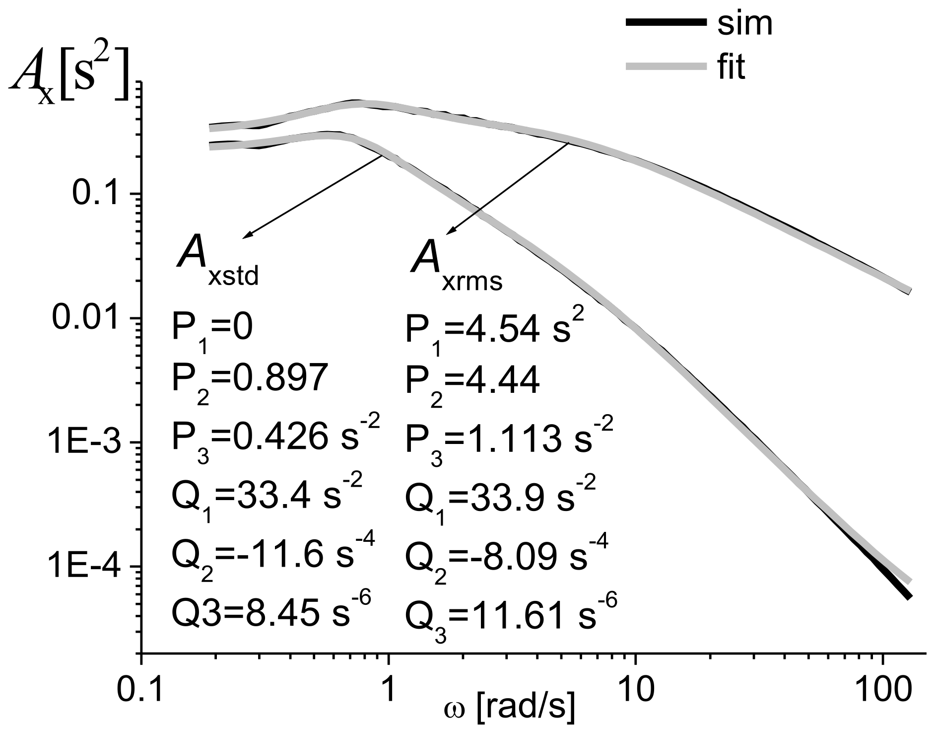
The values of transmissibility factors ${\tilde{A}}_{\mathrm{xrms}}\left({\mathrm{\omega }}_i\right)=\frac{{\mathrm{\Psi }}_{\mathrm{x}}\left({\mathrm{\omega }}_i\right)}{{\mathrm{\sigma }}_{{\mathrm{p}}_{0i}}}=\frac{\sqrt{2}\hspace{0.17em}{\mathrm{\Psi }}_{\mathrm{x}}\left({\mathrm{\omega }}_i\right)}{{\mathrm{P}}_0},\hspace{0.17em}\hspace{0.17em}\hspace{0.17em}\hspace{0.17em}i=\overline{1,N\hspace{0.17em}},$ and ${\tilde{A}}_{\mathrm{xstd}}\left({\mathrm{\omega }}_i\right)=\frac{{\mathrm{\sigma }}_{\mathrm{x}}\left({\mathrm{\omega }}_i\right)}{{\mathrm{\sigma }}_{{\mathrm{p}}_{0i}}}=\frac{\sqrt{2}{\mathrm{\sigma }}_{\mathrm{x}}\left({\mathrm{\omega }}_i\right)}{{\mathrm{P}}_0},\hspace{0.17em}\hspace{0.17em}\hspace{0.17em}i=\overline{1,N}$ corresponding to rms ${\mathrm{\Psi }}_{\mathrm{x}}$ and std ${\mathrm{\sigma }}_{\mathrm{x}}$ of relative displacement $x\left(t\right)$ are obtained by numerical integrations. These values can be approximated by rational expressions having the form

$$A_{\mathrm{x}}\left(\mathrm{\omega }\right)\hspace{0.17em}\hspace{0.17em}=\sqrt{\frac{P_1{\mathrm{\omega }}^4+P_2{\mathrm{\omega }}^2+P_3}{{\mathrm{\omega }}^6+Q_1{\mathrm{\omega }}^4+Q_2{\mathrm{\omega }}^2+Q_3}}$$

(35)

The transmissibility factor is written as

$$A_{\mathrm{x}}\left(\mathrm{\omega }\right)\hspace{0.17em}\hspace{0.17em}=\left|\frac{b_0{\left(\mathrm{i}\mathrm{\omega }\right)}^2+b_1\left(\mathrm{i}\mathrm{\omega }\right)+b_2}{{\left(\mathrm{i}\mathrm{\omega }\right)}^3+a_1{\left(\mathrm{i}\mathrm{\omega }\right)}^2+a_2\left(\mathrm{i}\mathrm{\omega }\right)+a_3}\right|=\sqrt{\frac{b_0^2{\mathrm{\omega }}^4+\left(b_1^2-2b_0{b}_2\right){\mathrm{\omega }}^2+b_2^2}{{\mathrm{\omega }}^6+\left(a_1^2-2a_2\right){\mathrm{\omega }}^4+\left(a_2-2a_1{a}_3\right){\mathrm{\omega }}^2+a_3^2}}$$

(36)

From relations (35) and (36) one can obtain the following algebraic systems of equations for unknown coefficients $b_0,b_1,b_2,a_1,\hspace{0.17em}{a}_2,a_3$:

$$\left\{\begin{array}{l}{b}_0^2=P_1\\ b_1^2-2b_0{b}_2=P_2\\ b_2^2=P_3\end{array}\right.,\hspace{0.17em}\hspace{0.17em}\hspace{0.17em}\left\{\begin{array}{l}\hspace{0.17em}{a}_1^2-2a_2=Q_1\\ a_2^2-2a_1{a}_3=\hspace{0.17em}{Q}_2\\ a_3^2\hspace{0.17em}=Q_3\end{array}\right.$$

(37)

The equations of the attached linear system having the same transmissibility factor (35) can be written as

$$\dot{u}=Au+c{p}_0$$

(38)

where

$$\begin{array}{c}\hspace{0.17em}{u}_1\left(t\right)=x\left(t\right),\\ A=\hspace{0.17em}\hspace{0.17em}\hspace{0.17em}\left[\hspace{0.17em}\begin{array}{ccc}0& 1& 0\\ 0& 0& 1\\ -a_3& -a_2& -a_1\end{array}\right]\hspace{0.17em},\hspace{0.17em}\hspace{0.17em}u=\left[\begin{array}{c}{u}_1\\ u_2\\ u_3\end{array}\right]\hspace{0.17em}\hspace{0.17em},\hspace{0.17em}\hspace{0.17em}c=\left[\begin{array}{c}{c}_1\\ c_2\\ c_3\end{array}\right],\hspace{0.17em}\hspace{0.17em}\hspace{0.17em}\left\{\begin{array}{l}{c}_1=b_0\\ c_2=b_1-a_1{c}_1\\ c_3=b_2-a_2{c}_1-a_1{c}_2\end{array}\right.\end{array}$$

(39)

The system (38) is asymptotically stable if $a_i>0,$ for $i=1,2,3.$ The covariance function and spectral density of system input $p_0\left(t\right)$ are given by (21). The attached system of stochastic differential equations with white noise excitation is given by

$$\dot{u}=Au+gz$$

(40)

where

$$\begin{array}{c}\begin{array}{l}\hspace{0.17em}{u}_1\left(t\right)=x,\hspace{0.17em}\hspace{0.17em}{u}_2\left(t\right)=\dot{x}\left(t\right),\hspace{0.17em}\hspace{0.17em}{u}_4=p_0\left(t\right),\hspace{0.17em}\hspace{0.17em}A=\hspace{0.17em}\hspace{0.17em}\hspace{0.17em}\left[\hspace{0.17em}\begin{array}{ccccc}0& 1& 0& c_1& 0\\ 0& 0& 1& c_2& 0\\ -a_3& -a_2& -a_1& c_3& 0\\ 0& 0& 0& 0& 1\\ 0& 0& 0& -a_5& -a_4\end{array}\right]\hspace{0.17em},\hspace{0.17em}\hspace{0.17em}u=\left[\begin{array}{c}{u}_1\\ u_2\\ u_3\\ u_4\\ u_5\end{array}\right]\hspace{0.17em}\hspace{0.17em},\hspace{0.17em}\hspace{0.17em}g=\left[\begin{array}{c}0\\ 0\\ 0\\ g_1\\ g_2\end{array}\right]\\ \hspace{0.17em}\hspace{0.17em}\hspace{0.17em}\hspace{0.17em}\hspace{0.17em}\hspace{0.17em}\hspace{0.17em}\hspace{0.17em}\hspace{0.17em}\hspace{0.17em}\hspace{0.17em}\hspace{0.17em}\hspace{0.17em}\hspace{0.17em}\hspace{0.17em}\hspace{0.17em}\hspace{0.17em}\hspace{0.17em}\hspace{0.17em}\hspace{0.17em}\hspace{0.17em}\hspace{0.17em}\hspace{0.17em}\hspace{0.17em}\hspace{0.17em}\hspace{0.17em}\hspace{0.17em}\hspace{0.17em}\hspace{0.17em}\hspace{0.17em}\hspace{0.17em}\hspace{0.17em}\hspace{0.17em}\hspace{0.17em}\end{array}\\ \hspace{0.17em}\hspace{0.17em}{a}_4=2a,\hspace{0.17em}\hspace{0.17em}{a}_5=a^2+b^2\hspace{0.17em},\hspace{0.17em}\hspace{0.17em}{g}_1={\mathrm{\sigma }}_0\sqrt{\frac{a}{\mathrm{\pi }}},\hspace{0.17em}\hspace{0.17em}{g}_2={\mathrm{\sigma }}_0\sqrt{\frac{a}{\mathrm{\pi }}}\left(\sqrt{a^2+b^2}-2a\hspace{0.17em}\right)\end{array}$$

(41)

The rms and std values of relative displacements of PWL system, ${\mathrm{\Psi }}_{\mathrm{x}}$ and ${\mathrm{\sigma }}_{\mathrm{x}}$, can be approximated as ${\mathrm{\Psi }}_{\mathrm{x}}\cong \sqrt{c_{11\hspace{0.17em}\mathrm{rms}}}$ and ${\mathrm{\sigma }}_{\mathrm{x}\hspace{0.17em}}\cong \sqrt{c_{11\hspace{0.17em}\mathrm{std}}}$. The values of $c_{11\hspace{0.17em}\mathrm{rms}}$ and $c_{11\hspace{0.17em}\mathrm{std}}$ are the first elements of covariance matrices $C_{\mathrm{rms}}\left(c_{ij\mathrm{rms}}\right),\hspace{0.17em}{C}_{\mathrm{std}}\left(c_{ij\mathrm{std}}\right),i,j=\overline{1,4}$, obtained by solving the Lyapunov Equation (34), corresponding to attached linear systems for the transmissibility factors $A_{\mathrm{xrms}}\left(\mathrm{\omega }\right)$ and $A_{\mathrm{xstd}}\left(\mathrm{\omega }\right)$, respectively. The mean displacement of asymmetric PWL system is approximated by

$$m_{\mathrm{xLyap}}\cong \sqrt{c_{11\hspace{0.17em}\mathrm{rms}}-c_{11\hspace{0.17em}\mathrm{std}}}\mathrm{sgn}\left(S\left(\gamma ,\mathrm{\beta },{\zeta }_1\right)\right)$$

(42)

8. Numerical Results

In this section, the statistical characteristics of simulated output are compared with those calculated by solving the Lyapunov Equation (34) for corresponding attached linear systems. The length and sampling interval of simulated filtered white noise input $p_0(t)$ were $T=100 \mathrm{s}$ and $\Delta t=0.001 \mathrm{s}$. The results obtained for the study cases, given in Table 2 for PWL asymmetric systems and for their linear equivalent system (${\zeta }_{\mathrm{e}}=0.5,\hspace{0.17em}{\mathrm{\omega }}_{\mathrm{e}}=2\mathrm{\pi }\hspace{0.17em}\mathrm{rad}/\mathrm{s}$), are presented in

Table 4. The std values and relative errors for absolute accelerations.

Case	$\begin{array}{c}{\mathit{\sigma }}_{{\ddot{\mathbf{x}}}_1\mathbf{sim}\hspace{0.17em}}\\ [{\mathbf{m}/\mathbf{s}}^2]\end{array}$	$\begin{array}{c}{\mathit{\sigma }}_{{\ddot{\mathbf{x}}}_1\mathbf{Lyap}\hspace{0.17em}}\\ [{\mathbf{m}/\mathbf{s}}^2]\end{array}$	Relative Error (%)	$\begin{array}{c}{\mathit{\sigma }}_{{\ddot{\mathbf{x}}}_1\mathbf{LinEq}\hspace{0.17em}}\\ [{\mathbf{m}/\mathbf{s}}^2]\end{array}$	Relative Error (%)
1	0.537	0.516	3.9	0.742	38
2	0.597	0.559	6.4	0.742	24
3	0.665	0.618	7.1	0.742	11
4	0.564	0.536	5	0.742	31
5	0.634	0.587	7.4	0.742	17
6	0.720	0.709	1.5	0.742	3

,

Table 5. The rms values and relative errors for relative displacements.

Case	$\begin{array}{c}{\mathbf{rms}}_{\mathbf{xsim}\hspace{0.17em}}\\ [\mathbf{m}]\end{array}$	$\begin{array}{c}{\mathbf{rms}}_{\mathbf{xLyap}\hspace{0.17em}}\\ [\mathbf{m}]\end{array}$	Relative Error (%)	$\begin{array}{c}{\mathbf{rms}}_{\mathbf{LinEq}\hspace{0.17em}}\\ [\mathbf{m}]\end{array}$	Relative Error (%)
1	0.181	0.185	0.022	0.013	0.928
2	0.0488	0.048	0.016	0.013	0.737
3	0.0277	0.026	0.061	0.013	0.535
4	0.0658	0.067	0.018	0.013	0.804
5	0.0285	0.028	0.018	0.013	0.546
6	0.0174	0.017	0.023	0.013	0.257

and

Table 6. The mean values and relative errors for relative displacements.

Case	$\begin{array}{c}{\mathit{m}}_{\mathbf{xsim}}\\ [\mathbf{m}]\end{array}$	$\begin{array}{c}{\mathit{c}}_{11}{}_{\mathbf{rms}\hspace{0.17em}}\\ [{\mathbf{m}}^2]\end{array}$	$\begin{array}{c}{\mathit{c}}_{11}{}_{\mathbf{std}}\\ [{\mathbf{m}}^2]\end{array}$	$\begin{array}{c}{\mathit{m}}_{\mathbf{xLyap}\hspace{0.17em}}\\ [\mathbf{m}]\end{array}$	Relative Error (%)	$\begin{array}{c}{\mathit{m}}_{\mathbf{x}}\\ [\mathbf{m}]\end{array}$
1	−0.167	0.0343	0.0019	−0.18	7.8	−0.168
2	−0.039	0.0023	0.0005	−0.042	7.7	−0.04
3	−0.02	0.0007	0.0002	−0.022	10	−0.02
4	−0.055	0.0045	0.0007	−0.062	12.7	−0.056
5	−0.02	0.0008	0.0003	−0.022	10	−0.021
6	0.009	0.0003	0.0002	0.01	11.1	0.009

.

The last column of Table 6 shows the mean values of displacement, evaluated by using in (8) the values $\hspace{0.17em}{\mathrm{m}}_{\left|\mathrm{x}\right|},m_{\left| \dot{\mathrm{x}}\right|}$ obtained by numerical integration of PWL equation of motion (6). It worth noting that the optimum value of damping ratio for a linear system with undamped eigenfrequency ${\mathrm{\omega }}_1=2\mathrm{\pi }\hspace{0.17em}\mathrm{rad}/\mathrm{s}$ and considered random input $p_0(t)$, is ${\zeta }_{\mathrm{opt}}=0.55$. The value of standard deviation of simulated acceleration output obtained in this case is ${\mathrm{\sigma }}_{{ \ddot{\mathrm{x}}}_1\hspace{0.17em}\mathrm{opt}}=0.741\hspace{0.17em}{\mathrm{m}/\mathrm{s}}^2.$

Table 4 shows that the simulated values ${\mathrm{\sigma }}_{{ \ddot{\mathrm{x}}}_1\mathrm{sim}\hspace{0.17em}}$ are better approximated by using the proposed method than the Gaussian equivalent linearization method. Therefore, in all case studies the asymmetric PWL systems provide better vibration isolation than the optimum linear system, for both considered random inputs (band limited and shape filtered white noise).

The results presented in Table 4 and Table 6 show that the relative errors of approximation between the results obtained by numerical integration of asymmetric PWL systems and those calculated by using the Lyapunov equation for linear attached systems are less than 7.5% for standard deviation of acceleration and less than 13% for mean value of displacement. As one can see, from Table 2 and Table 6, as nonlinearity increases, the mean value displacement is better approximated. It should be mentioned that the Gaussian equivalent linearization method cannot provide any information about the drift of sprung mass average position in dynamic regime, as it is shown in Table 5.

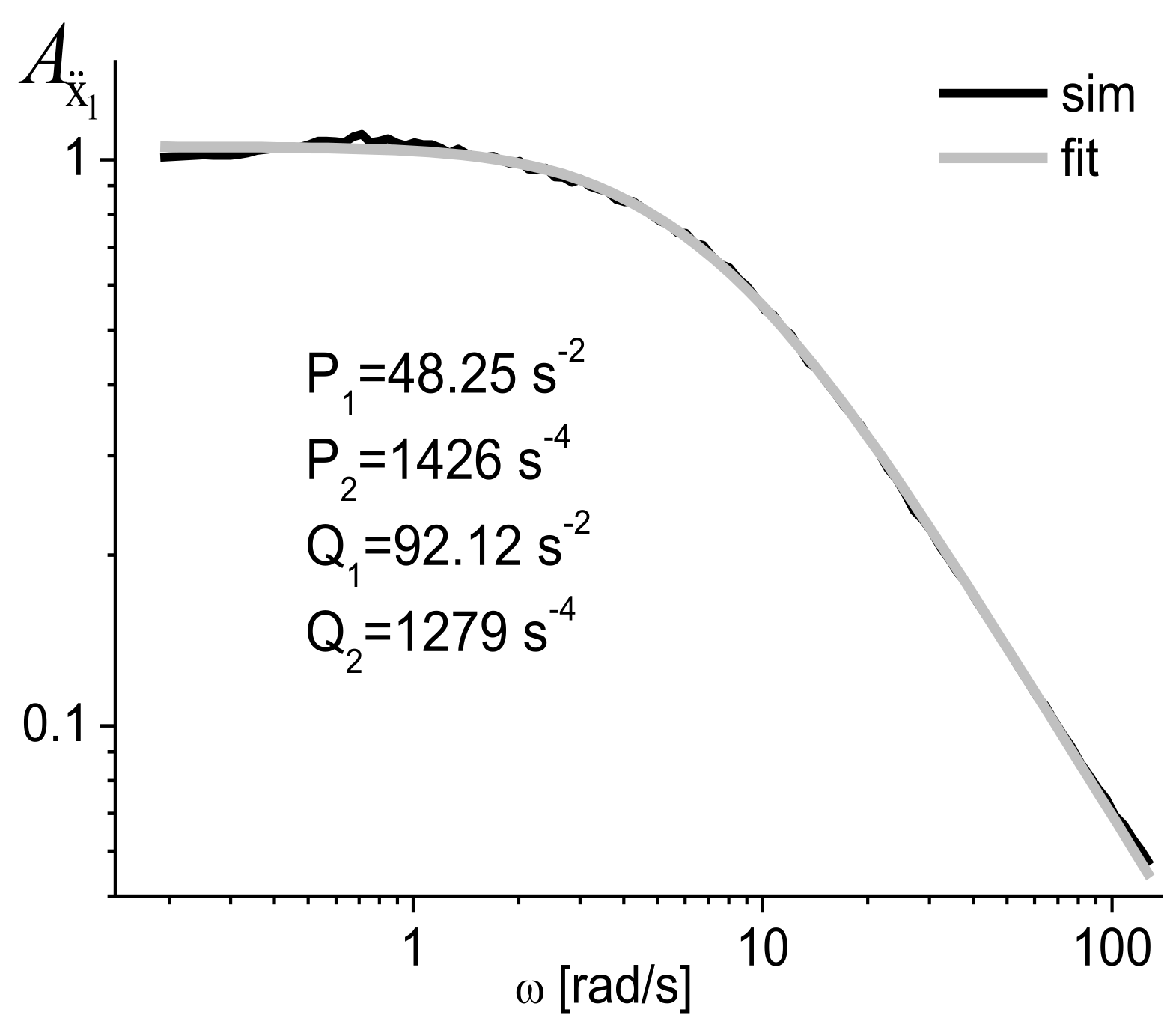
In order to illustrate the application of presented method, the case 1 from Table 2, which display the strongest nonlinearity, has been chosen. In Figure 8 and Figure 9 are plotted the transmissibility factors, simulated and fitted for this case, as well as the values of parameters from fitting the curves given by the expressions (27) and (35).

In

Table 7. Coefficients of attached linear system for std acceleration.

$\begin{array}{c}{\mathit{a}}_1\\ {[\mathbf{s}}^{-1}]\end{array}$	$\begin{array}{c}{\mathit{a}}_2\\ {[\mathbf{s}}^{-2}]\end{array}$	${\mathit{c}}_1$	$\begin{array}{c}{\mathit{c}}_2\\ {[\mathbf{s}}^{-1}]\end{array}$	$\begin{array}{c}{\mathit{c}}_{11}\\ {[\mathbf{m}}^2{\mathbf{s}}^{-4}]\end{array}$
13.07	37.35	6.96	−130.4	0.265

and

Table 8. Coefficients of attached linear system for std and rms displacement.

	$\begin{array}{c}{\mathit{a}}_1\\ {[\mathbf{s}}^{-1}]\end{array}$	$\begin{array}{c}{\mathit{a}}_2\\ {[\mathbf{s}}^{-2}]\end{array}$	$\begin{array}{c}{\mathit{a}}_3\\ {[\mathbf{s}}^{-3}]\end{array}$	${\mathit{c}}_1$	$\begin{array}{c}{\mathit{c}}_2\\ {[\mathbf{s}}^{-1}]\end{array}$	$\begin{array}{c}{\mathit{c}}_2\\ {[\mathbf{s}}^{-2}]\end{array}$	$\begin{array}{c}{\mathit{c}}_{11}\\ {[\mathbf{m}}^2]\end{array}$	$\begin{array}{c}{\left|{\mathit{m}}_{\mathbf{x}}\right|}_{\mathbf{Lyap}}\\ [\mathbf{m}]\end{array}$
Coefficients for std disp	6.45	5.05	2.82	0.0158	−1.036	7.236	0.0019	0.18
Coefficients for rms disp	6.8	6.19	3.41	2.13	−17.5	106.8	0.0343

are given the coefficients of attached linear systems corresponding to acceleration and displacement, obtained by solving the algebraic Equations (29), (31), (37) and (39) for parameters shown in Figure 8 and Figure 9.

In the last column of these tables are given the values of elements $c_{11}$ from covariance matrices obtained by solving the Lyapunov Equation (34), for the corresponding attached linear systems. Using these coefficients, are obtained the values of std acceleration ${\mathrm{\sigma }}_{{ \ddot{\mathrm{x}}}_1\mathrm{Lyap}\hspace{0.17em}}=\sqrt{c_{11}}=0.515$ ms⁻² and the mean value of displacement $m_{\mathrm{x}}{}_{\mathrm{Lyap}}\cong -\sqrt{c_{11\hspace{0.17em}\mathrm{rms}}-c_{11\hspace{0.17em}\mathrm{std}}}=-0.18$ m, according to (8). 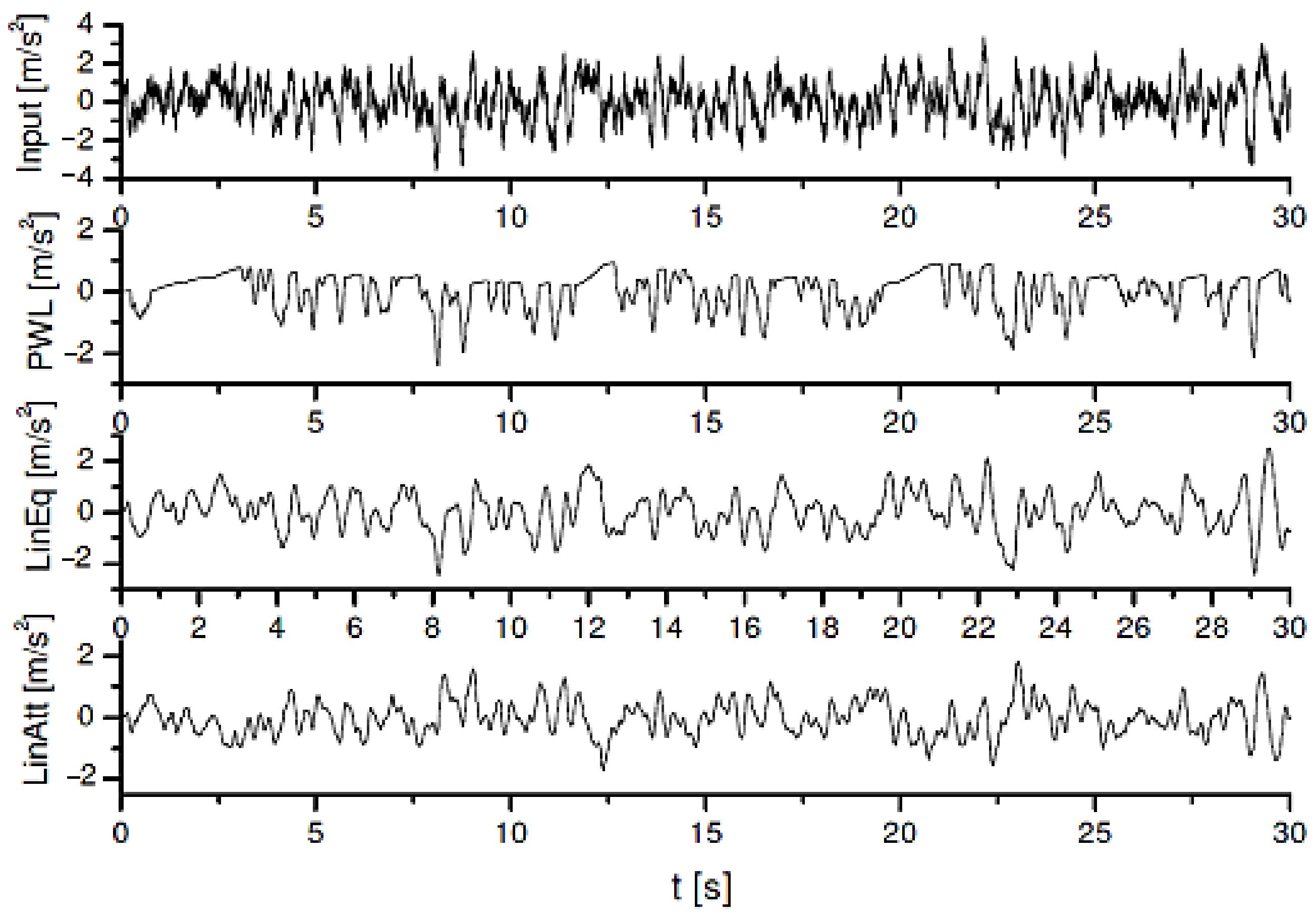Figure 10 shows the first 30 s from the simulated time histories of input, acceleration and displacements outputs for PWL, attached linear (rms for displacement) and linear equivalent systems, obtained for case study 1.

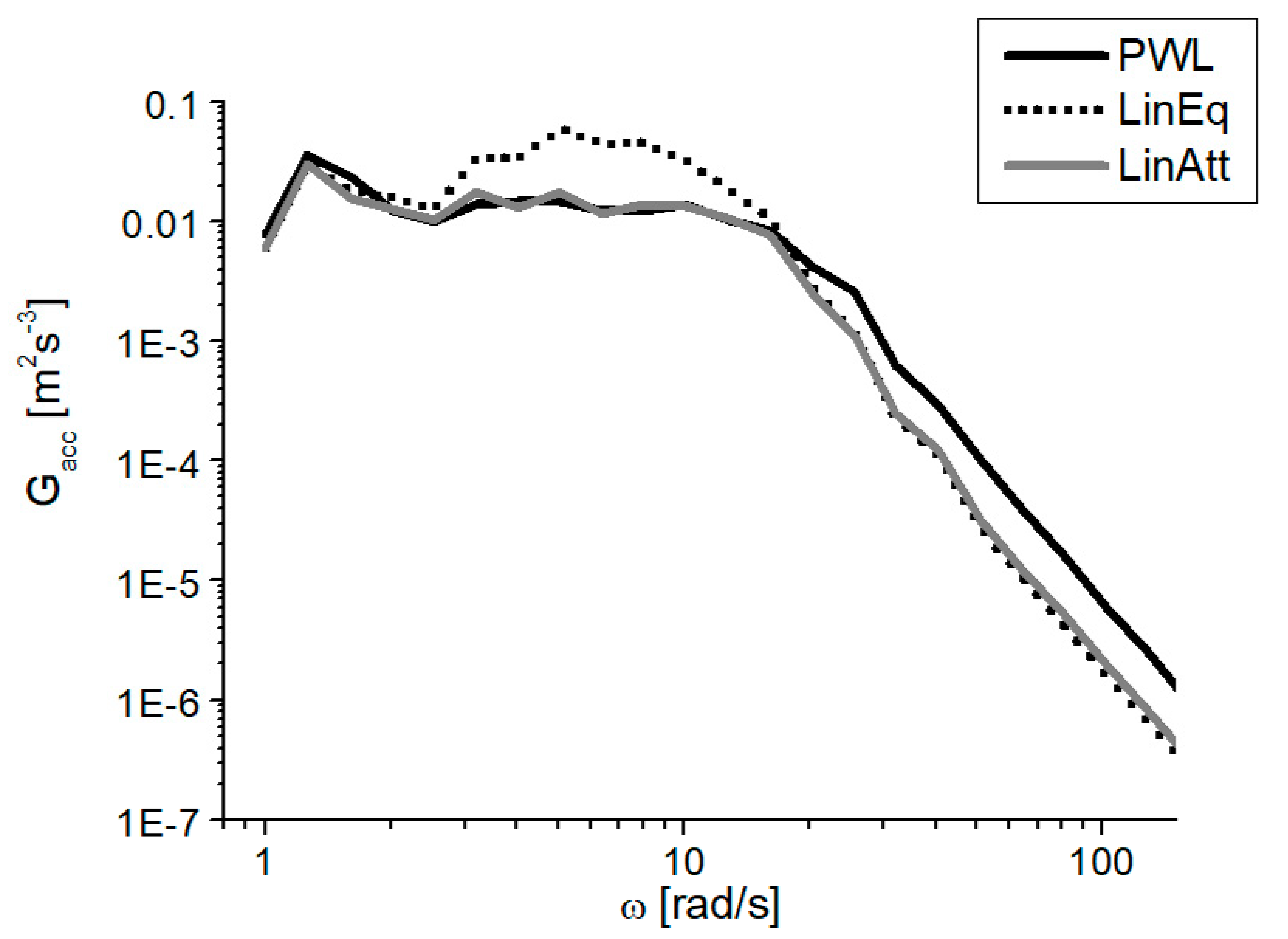
In Figure 11 are plotted the spectral densities of acceleration output, determined by 1/3 octave band-pass filtering for PWL, linear equivalent and the attached linear systems.

The relative errors between the areas under spectral densities that represent the variances of acceleration, given in

Table 9. Variances of acceleration for PWL, LinEq and LinAtt systems.

System	Area Gacc [m2/s4]	Relative Error %
PWL	0.254	-
LinEq	0.503	98
LinAtt	0.23	9.4

, advocate the efficiency of the proposed method.

9. Conclusions

The dynamic response of piecewise linear systems with asymmetric damping and stiffness for random inputs is approximated by a method based on transmissibility factors. The application of this method does not require the numerical simulation of input and output time histories, except for obtaining the transmissibility factors by using harmonic inputs. Using these frequency characteristics, a stochastic linear system is attached for each variable of interest. The statistical parameters of the studied output corresponding to random excitations having rational spectral densities are determined by solving the associated Lyapunov equation.

The obtained results are compared with those determined by the numerical integration of asymmetric PWL response. The relative errors show the efficiency and applicability of this method for PWL systems. In addition, this approach allows the realization of vibration isolation systems with better performance than those with linear characteristics. Using the attached linear systems for rms and std displacement, the shift of sprung mass average position in dynamic regime, due to damping or stiffness asymmetry, can be predicted with a good accuracy for stationary random input.