Author Contributions
Data curation, J.R.; formal analysis, J.R., M.A.R., P.L.C. and J.A.; investigation, J.R., M.A.R., P.L.C.; methodology, J.R., M.A.R., P.L.C. and J.A.; writing—original draft, J.R., M.A.R., P.L.C. and J.A.; writing—review and editing, M.A.R., P.L.C. and J.A.; funding acquisition, J.R., M.A.R. and J.A. All authors have read and agreed to the published version of the manuscript.
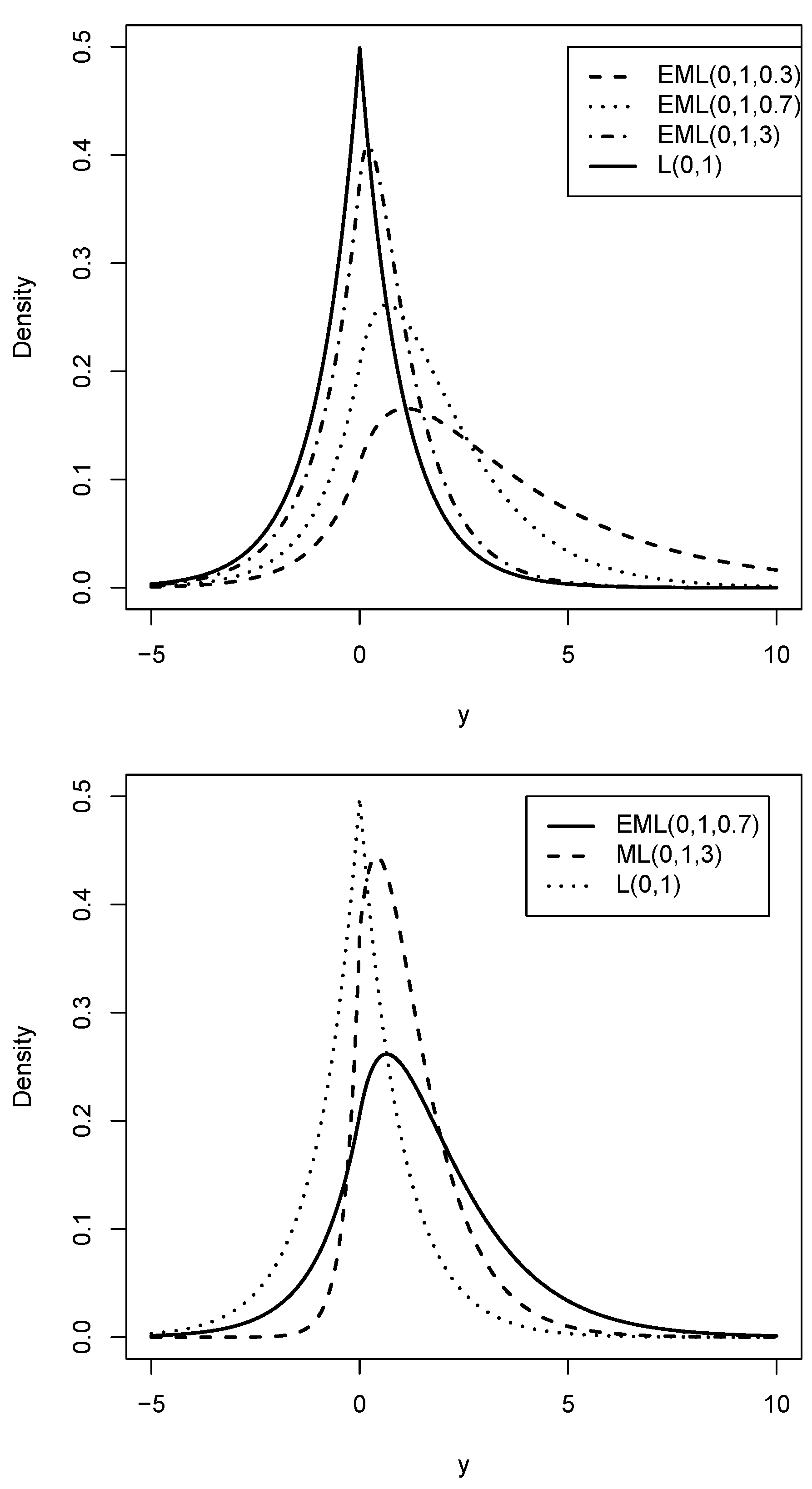
Figure 1.
Graphical comparison of EML distributions with L for different values of (upper) and with ML and L (lower).
Figure 1.
Graphical comparison of EML distributions with L for different values of (upper) and with ML and L (lower).
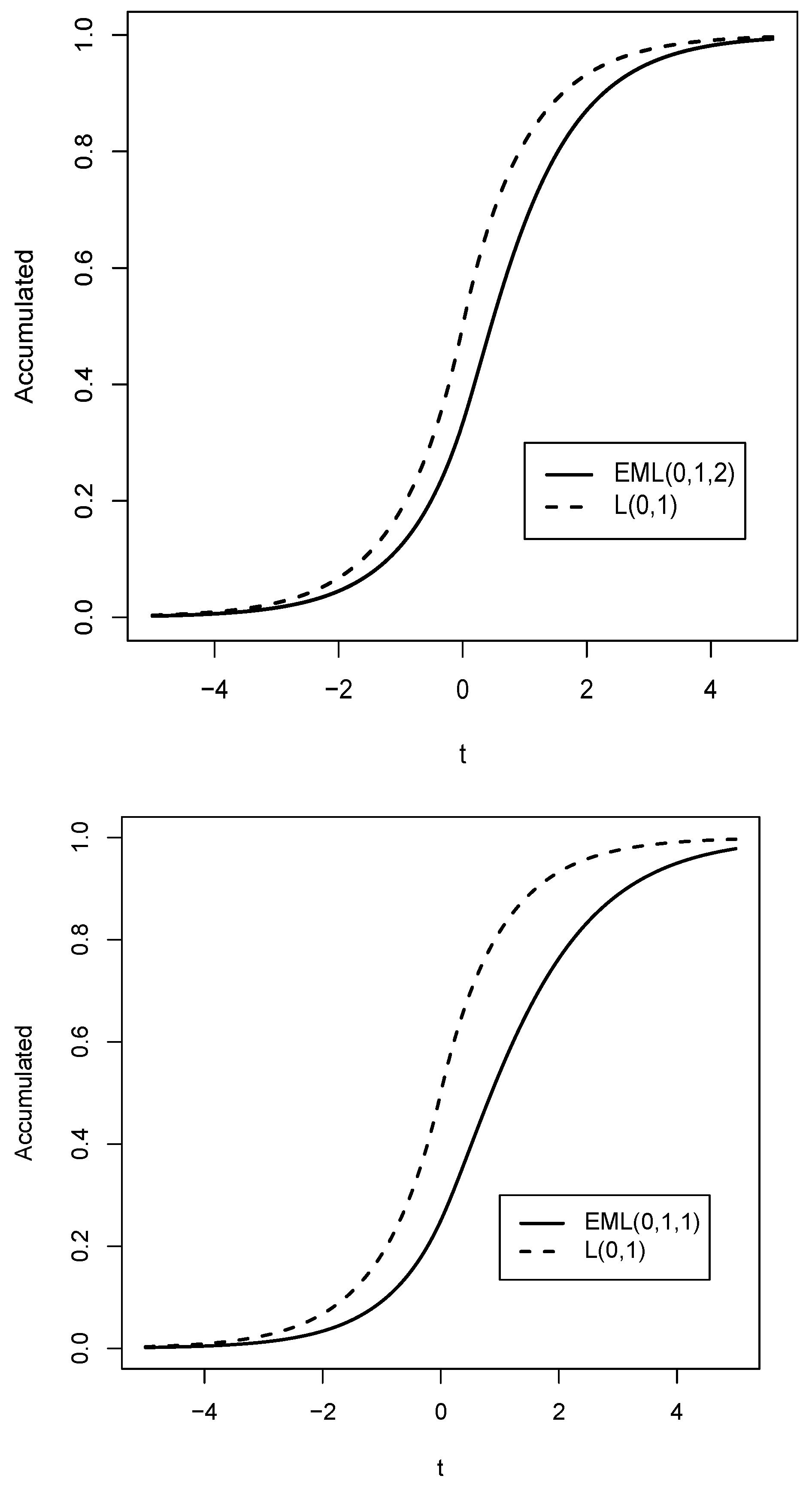
Figure 2.
Comparison of the cdf of the distribution (solid line) for (upper) and (lower) with the cdf of the distribution L (dashed line).
Figure 2.
Comparison of the cdf of the distribution (solid line) for (upper) and (lower) with the cdf of the distribution L (dashed line).
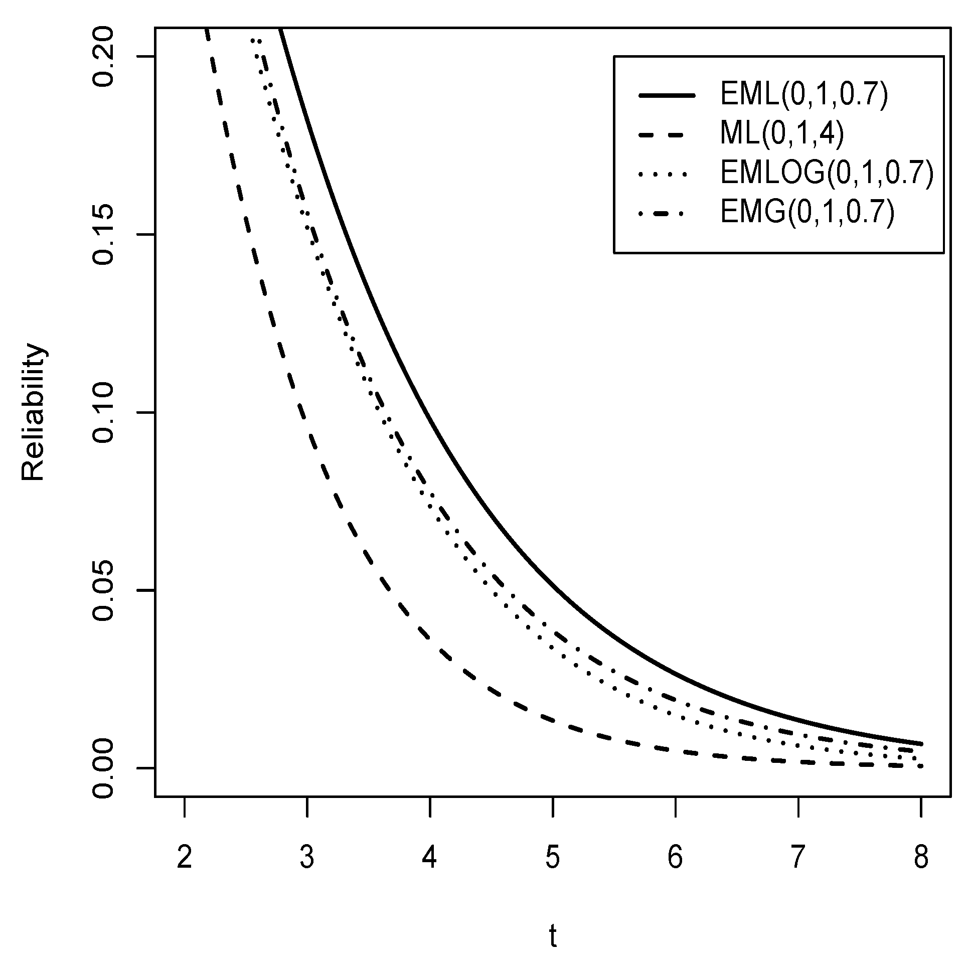
Figure 3.
Comparison of the reliability function of the distribution (solid line) for with the reliability function of the , , and distributions (dashed line, dotted line, dash-dotted line).
Figure 3.
Comparison of the reliability function of the distribution (solid line) for with the reliability function of the , , and distributions (dashed line, dotted line, dash-dotted line).
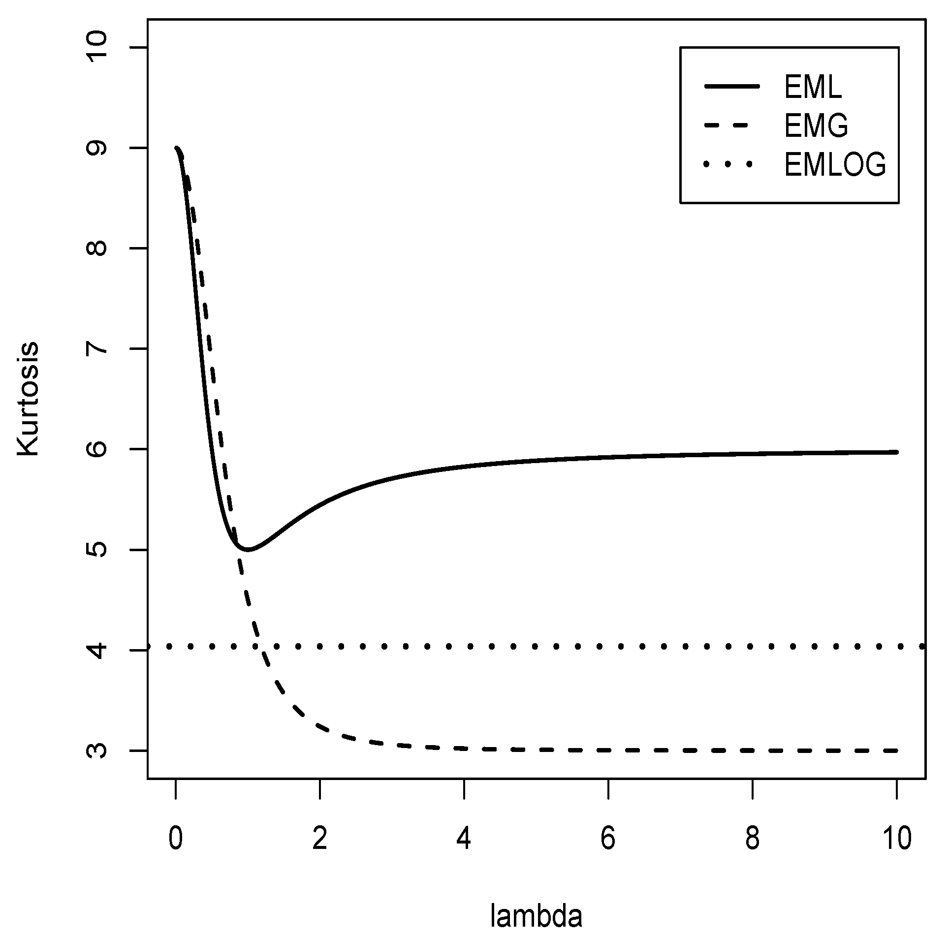
Figure 4.
Graphical comparison of the kurtosis coefficient between the exponentially modified Laplace distribution (solid line), the exponentially modified Gaussian distribution (dashed line), and the exponentially modified logistic distribution (dotted line).
Figure 4.
Graphical comparison of the kurtosis coefficient between the exponentially modified Laplace distribution (solid line), the exponentially modified Gaussian distribution (dashed line), and the exponentially modified logistic distribution (dotted line).
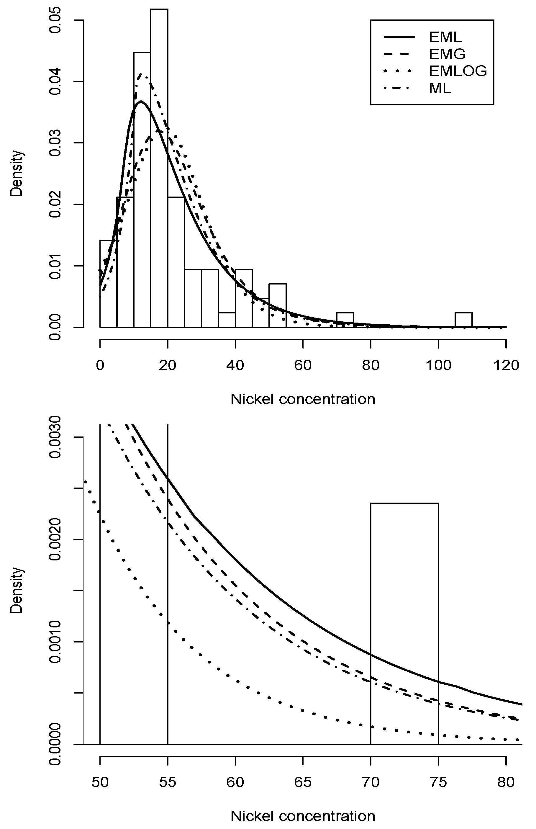
Figure 5.
Histogram (upper) and tail (lower) for nickel concentration data set. Overlaid on top is the density with parameters estimated via MLE (solid line), exponentially modified Gaussian density with parameters estimated via MLE (dotted line), exponentially modified logistic (dashed line), and modified Laplace (dash-dotted line).
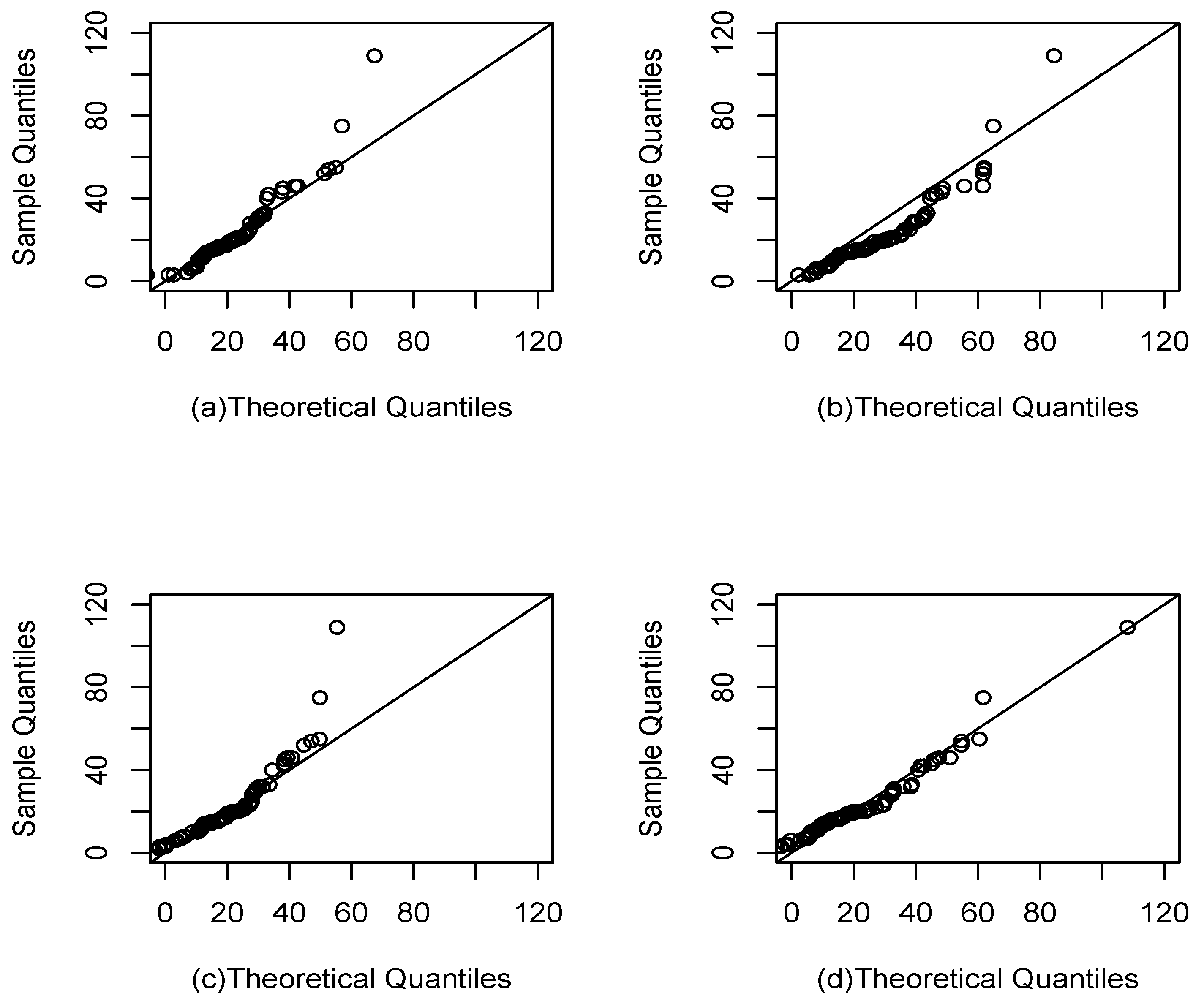
Figure 6.
QQ plot for nickel concentration data set. The modified Laplace density (a), exponentially modified logistic density (b), exponentially modified Gaussian density (c), and exponentially modified Laplace density (d).
Figure 6.
QQ plot for nickel concentration data set. The modified Laplace density (a), exponentially modified logistic density (b), exponentially modified Gaussian density (c), and exponentially modified Laplace density (d).
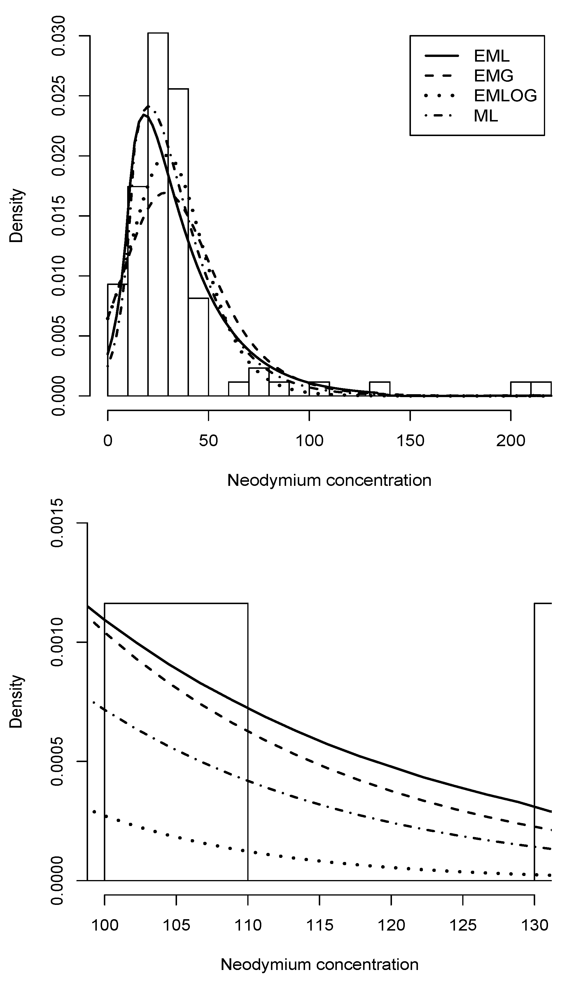
Figure 7.
Histogram (upper) and tail (lower) for the neodymium concentration data set. The first graph shows the densities of the exponentially modified Laplace (solid line), Gaussian modified exponentially (dashed line), exponentially modified logistic (dotted line), and modified Laplace (dash-dotted line) distributions, with their parameters estimated by MLE.
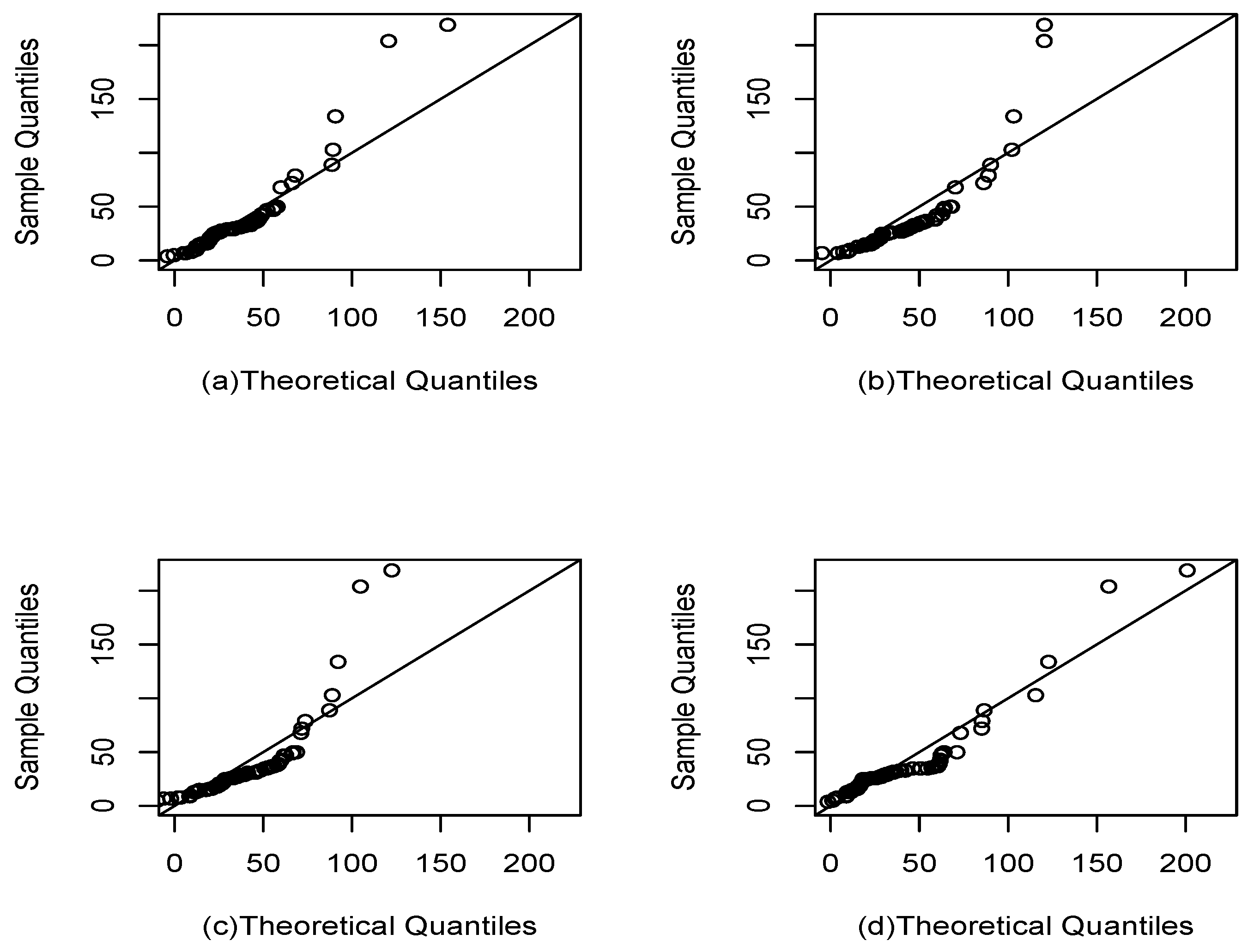
Figure 8.
QQ plot for the neodymium concentration data set. The modified Laplace density (a), exponentially modified logistic density (b), exponentially modified Gaussian density (c), and exponentially modified Laplace density (d).
Figure 8.
QQ plot for the neodymium concentration data set. The modified Laplace density (a), exponentially modified logistic density (b), exponentially modified Gaussian density (c), and exponentially modified Laplace density (d).
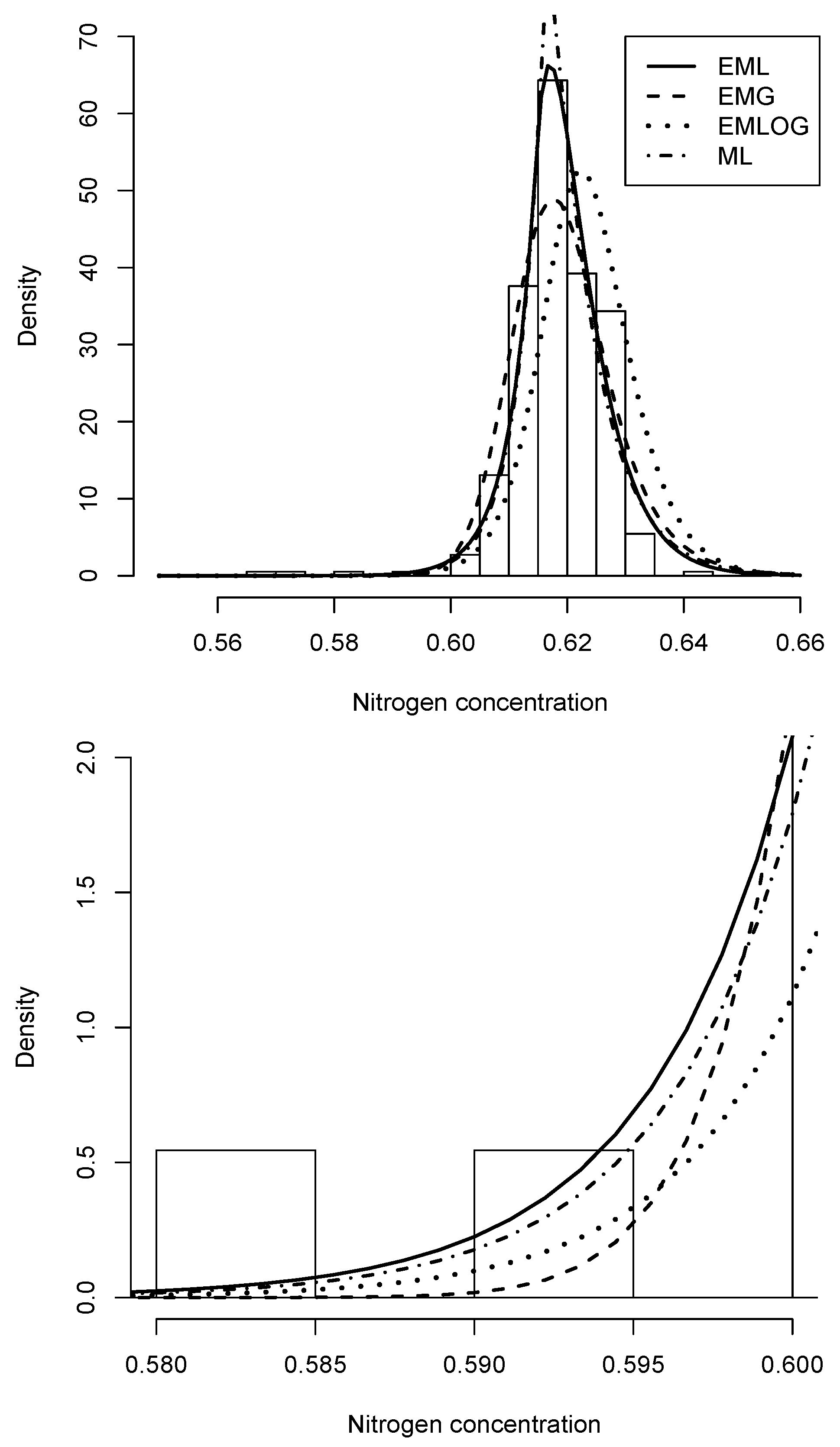
Figure 9.
Histogram (upper) and tail (lower) for nitrogen concentration data set. The first graph shows the densities of exponentially modified Laplace (solid line), Gaussian modified exponentially (dashed line), exponentially modified logistic (dotted line) and modified Laplace (dash-dotted line) distributions, with their parameters estimated by MLE.
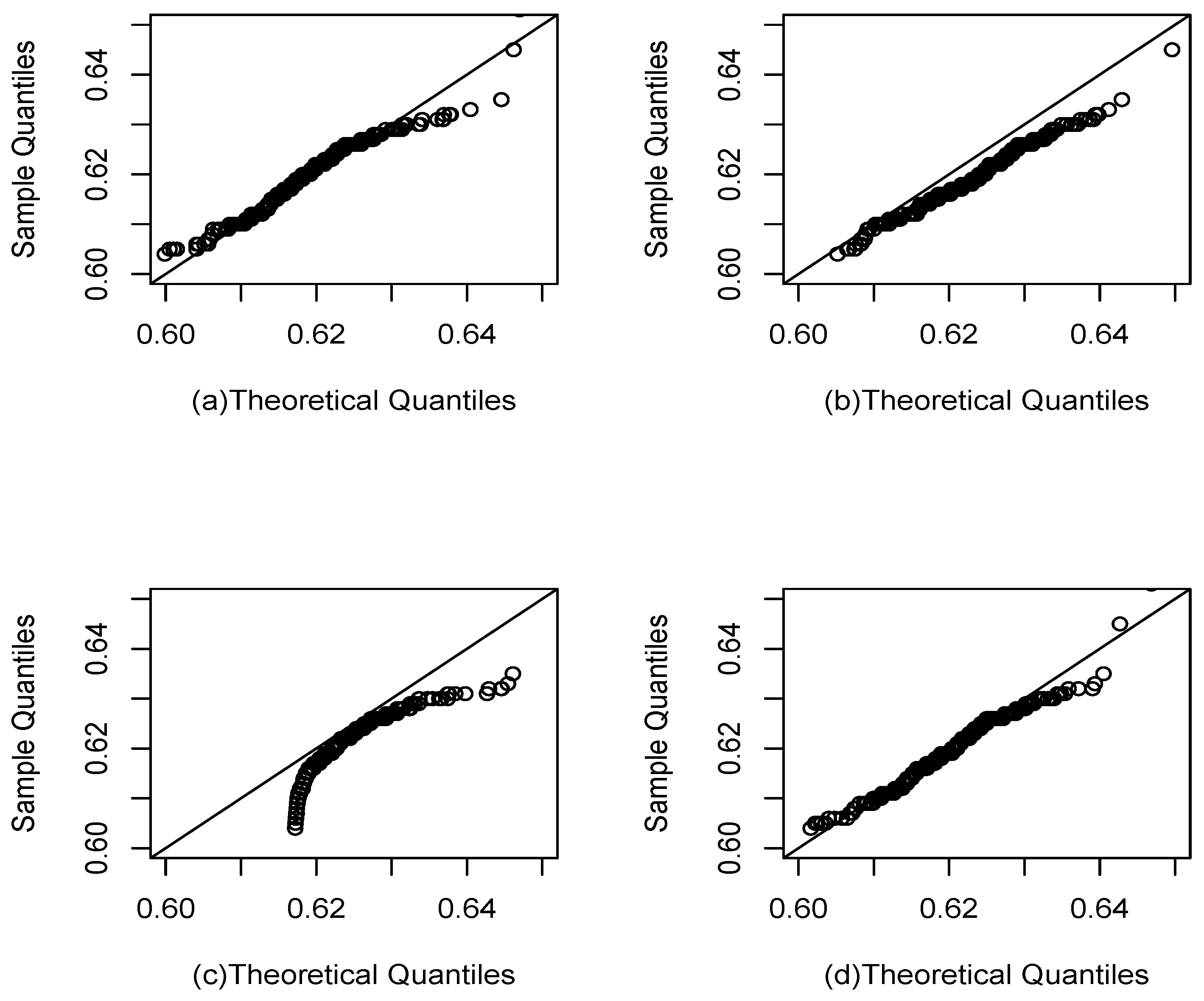
Figure 10.
QQ plot for Nitrogen concentration data set. The density (a), (b), density (c), and (d).
Figure 10.
QQ plot for Nitrogen concentration data set. The density (a), (b), density (c), and (d).
Table 1.
Reliability function comparison for distributions , , , and .
Table 1.
Reliability function comparison for distributions , , , and .
| Distribution | | | | | | | |
|---|
| 0.2444 | 0.1543 | 0.0958 | 0.0530 | 0.0361 | 0.0220 | 0.0134 |
| 0.2878 | 0.2116 | 0.1517 | 0.1065 | 0.0735 | 0.0501 | 0.0377 |
| 0.3073 | 0.2202 | 0.1561 | 0.1102 | 0.0775 | 0.0547 | 0.0385 |
| 0.3256 | 0.2449 | 0.1820 | 0.1339 | 0.0978 | 0.0711 | 0.0515 |
Table 2.
ME simulation of 1000 iterations of the model .
Table 2.
ME simulation of 1000 iterations of the model .
| n | | | | | | | | | | | | | | | |
|---|
| 50 | 0 | 1 | 0.3 | 0.0341 | 0.1189 | 0.4661 | 93.9 | 1.0341 | 0.1189 | 0.4661 | 93.9 | 0.3341 | 0.1189 | 0.4661 | 93.9 |
| 100 | 0 | 1 | 0.3 | 0.0123 | 0.0650 | 0.2548 | 95.2 | 1.0123 | 0.0650 | 0.2548 | 95.2 | 0.3123 | 0.0650 | 0.2548 | 95.2 |
| 200 | 0 | 1 | 0.3 | 0.0066 | 0.0411 | 0.1612 | 94.7 | 1.0066 | 0.0411 | 0.1612 | 94.7 | 0.3066 | 0.0411 | 0.1612 | 94.7 |
| 500 | 0 | 1 | 0.3 | 0.0036 | 0.0245 | 0.0959 | 94.6 | 1.0036 | 0.0245 | 0.0959 | 94.6 | 0.3036 | 0.0245 | 0.0959 | 94.6 |
| 50 | 0 | 1 | 0.7 | −0.1249 | 0.2589 | 1.0150 | 97.4 | 0.8751 | 0.2589 | 1.0150 | 97.4 | 0.5751 | 0.2589 | 1.0150 | 97.4 |
| 100 | 0 | 1 | 0.7 | −0.1162 | 0.2293 | 0.8989 | 96.1 | 0.8838 | 0.2293 | 0.8989 | 96.1 | 0.5838 | 0.2293 | 0.8989 | 96.1 |
| 200 | 0 | 1 | 0.7 | −0.0785 | 0.1901 | 0.7451 | 91.0 | 0.9215 | 0.1901 | 0.7451 | 91.0 | 0.6215 | 0.1901 | 0.7451 | 91.0 |
| 500 | 0 | 1 | 0.7 | −0.0434 | 0.1540 | 0.6038 | 93.8 | 0.9566 | 0.1540 | 0.6038 | 93.8 | 0.6566 | 0.1540 | 0.6038 | 93.8 |
| 50 | 0 | 1 | 1 | −0.1006 | 0.3208 | 1.2576 | 92.7 | 0.8994 | 0.3208 | 1.2576 | 92.7 | 0.8994 | 0.3208 | 1.2576 | 92.7 |
| 100 | 0 | 1 | 1 | −0.0399 | 0.2174 | 0.8522 | 96.7 | 0.9601 | 0.2174 | 0.8522 | 96.7 | 0.9601 | 0.2174 | 0.8522 | 96.7 |
| 200 | 0 | 1 | 1 | −0.0149 | 0.1373 | 0.5381 | 97.3 | 0.9851 | 0.1373 | 0.5381 | 97.3 | 0.9851 | 0.1373 | 0.5381 | 97.3 |
| 500 | 0 | 1 | 1 | −0.0038 | 0.0760 | 0.2978 | 93.7 | 0.9962 | 0.0760 | 0.2978 | 93.7 | 0.9962 | 0.0760 | 0.2978 | 93.7 |
| 50 | 0 | 1 | 1.2 | −0.0525 | 0.2984 | 1.1698 | 96.6 | 0.9475 | 0.2984 | 1.1698 | 96.6 | 1.1475 | 0.2984 | 1.1698 | 96.6 |
| 100 | 0 | 1 | 1.2 | −0.0114 | 0.1827 | 0.7161 | 98.1 | 0.9886 | 0.1827 | 0.7161 | 98.1 | 1.1886 | 0.1827 | 0.7161 | 98.1 |
| 200 | 0 | 1 | 1.2 | 0.0004 | 0.1118 | 0.4383 | 96.0 | 1.0004 | 0.1118 | 0.4383 | 96.0 | 1.2004 | 0.1118 | 0.4383 | 96.0 |
| 500 | 0 | 1 | 1.2 | −0.0024 | 0.0637 | 0.2499 | 94.3 | 0.9976 | 0.0637 | 0.2499 | 94.3 | 1.1976 | 0.0637 | 0.2499 | 94.3 |
| 50 | −1 | 2 | 0.3 | −0.9902 | 0.0641 | 0.2512 | 94.7 | 2.0098 | 0.0641 | 0.2512 | 94.7 | 0.3098 | 0.0641 | 0.2512 | 94.7 |
| 100 | −1 | 2 | 0.3 | −0.9923 | 0.0462 | 0.1810 | 94.9 | 2.0077 | 0.0462 | 0.1810 | 94.9 | 0.3077 | 0.0462 | 0.1810 | 94.9 |
| 200 | −1 | 2 | 0.3 | −0.9958 | 0.0301 | 0.1181 | 94.7 | 2.0042 | 0.0301 | 0.1181 | 94.7 | 0.3042 | 0.0301 | 0.1181 | 94.7 |
| 500 | −1 | 2 | 0.3 | −0.9987 | 0.0185 | 0.0723 | 94.8 | 2.0013 | 0.0185 | 0.0723 | 94.8 | 0.3013 | 0.0185 | 0.0723 | 94.8 |
Table 3.
MLE simulation of 1000 iterations of the model .
Table 3.
MLE simulation of 1000 iterations of the model .
| n | | | | | | | | | | | | | | | |
|---|
| 50 | 0 | 1 | 0.3 | 0.0470 | 0.5226 | 2.0486 | 93.6 | 0.9327 | 0.3885 | 1.5229 | 94.2 | 0.3175 | 0.2096 | 0.8216 | 96.2 |
| 100 | 0 | 1 | 0.3 | 0.0326 | 0.3439 | 1.3480 | 94.2 | 0.9822 | 0.2534 | 0.9933 | 94.8 | 0.3081 | 0.1139 | 0.4463 | 94.9 |
| 200 | 0 | 1 | 0.3 | 0.0093 | 0.2300 | 0.9015 | 94.5 | 0.9937 | 0.1746 | 0.6843 | 95.4 | 0.3035 | 0.0706 | 0.2769 | 95.1 |
| 500 | 0 | 1 | 0.3 | −0.0061 | 0.1408 | 0.5521 | 95.0 | 0.9956 | 0.1087 | 0.4260 | 95.3 | 0.2999 | 0.0444 | 0.1740 | 94.6 |
| 50 | 0 | 1 | 0.7 | −0.0023 | 0.3834 | 1.5031 | 94.5 | 0.9491 | 0.2611 | 1.0237 | 95.6 | 0.7974 | 0.5617 | 2.2017 | 94.8 |
| 100 | 0 | 1 | 0.7 | 0.0255 | 0.2872 | 1.1257 | 94.1 | 0.9692 | 0.1913 | 0.7498 | 94.6 | 0.7607 | 0.3987 | 1.5630 | 95.7 |
| 200 | 0 | 1 | 0.7 | 0.0261 | 0.2011 | 0.7882 | 94.9 | 1.0004 | 0.1396 | 0.5471 | 95.9 | 0.7527 | 0.2750 | 1.0779 | 96.1 |
| 500 | 0 | 1 | 0.7 | 0.0084 | 0.1211 | 0.4747 | 95.2 | 0.9968 | 0.0829 | 0.3249 | 94.9 | 0.7130 | 0.1229 | 0.4816 | 94.8 |
| 50 | 0 | 1 | 1.0 | −0.0149 | 0.3755 | 1.4718 | 95.4 | 0.9182 | 0.2369 | 0.9286 | 93.7 | 1.2052 | 1.0383 | 4.0701 | 93.8 |
| 100 | 0 | 1 | 1.0 | 0.0176 | 0.2805 | 1.0997 | 94.7 | 0.9654 | 0.1697 | 0.6653 | 95.0 | 1.1874 | 0.8215 | 3.2204 | 93.7 |
| 200 | 0 | 1 | 1.0 | 0.0248 | 0.2150 | 0.8428 | 94.6 | 0.9898 | 0.1266 | 0.4962 | 94.3 | 1.1528 | 0.6274 | 2.4595 | 94.8 |
| 500 | 0 | 1 | 1.0 | 0.0106 | 0.1361 | 0.5337 | 94.7 | 0.9924 | 0.0842 | 0.3300 | 94.7 | 1.0473 | 0.3208 | 1.2574 | 96.5 |
| 50 | 0 | 1 | 1.2 | −0.0644 | 0.3430 | 1.3444 | 94.8 | 0.8979 | 0.2139 | 0.8385 | 92.1 | 1.2577 | 0.9488 | 3.7195 | 95.5 |
| 100 | 0 | 1 | 1.2 | −0.0013 | 0.2758 | 1.0812 | 94.6 | 0.9568 | 0.1629 | 0.6384 | 93.5 | 1.3821 | 0.9002 | 3.5287 | 93.1 |
| 200 | 0 | 1 | 1.2 | 0.0090 | 0.2123 | 0.8322 | 94.9 | 0.9849 | 0.1200 | 0.4704 | 95.1 | 1.3675 | 0.7209 | 2.8259 | 94.2 |
| 500 | 0 | 1 | 1.2 | 0.0123 | 0.1373 | 0.5383 | 94.5 | 0.9969 | 0.0792 | 0.3104 | 94.6 | 1.2831 | 0.4290 | 1.6819 | 95.5 |
| 50 | −1 | 2 | 0.3 | −0.8821 | 0.9899 | 3.8805 | 95.0 | 1.8777 | 0.7352 | 2.8819 | 93.8 | 0.3135 | 0.2027 | 0.7946 | 97.3 |
| 100 | −1 | 2 | 0.3 | −0.9601 | 0.6781 | 2.6582 | 96.1 | 1.9483 | 0.5054 | 1.9813 | 94.6 | 0.3071 | 0.1150 | 0.4507 | 95.5 |
| 200 | −1 | 2 | 0.3 | −0.9681 | 0.4653 | 1.8239 | 95.0 | 1.9917 | 0.3324 | 1.3030 | 94.9 | 0.3061 | 0.0702 | 0.2754 | 94.5 |
| 500 | −1 | 2 | 0.3 | −0.9883 | 0.2807 | 1.1004 | 94.6 | 1.9960 | 0.2197 | 0.8612 | 94.7 | 0.3021 | 0.0448 | 0.1755 | 94.9 |
Table 4.
Summary Statistics for the Nickel Concentration Data Set.
Table 4.
Summary Statistics for the Nickel Concentration Data Set.
| n | | | | |
|---|
| 85 | 21.3372 | 16.6391 | 2.3559 | 11.1917 |
Table 5.
Maximum likelihood estimators for , , , and models for the soil nickel concentration data set, with their corresponding standard deviations in parentheses and comparison criteria AIC, BIC, CAIC, and HQIC.
Table 5.
Maximum likelihood estimators for , , , and models for the soil nickel concentration data set, with their corresponding standard deviations in parentheses and comparison criteria AIC, BIC, CAIC, and HQIC.
| Parameter Estimates | | | | |
|---|
| 11.0020 (0.0657) | 18.9149 (1.4048) | 10.0433 (0.0771) | 7.020 (0.0462) |
| 11.6843 (1.21645) | 7.6833 (0.7231) | 9.0165 (0.0766) | 5.1452 (0.0258) |
| 2.2279 (0.2418) | | 0.7810 (0.0610) | 0.3733 (0.0443) |
| AIC | 687.022 | 699.207 | 685.0531 | 682.053 |
| BIC | 694.385 | 704.092 | 692.381 | 689.381 |
| CAIC | 695.548 | 705.092 | 693.381 | 690.381 |
| HQIC | 690.168 | 701.172 | 688.001 | 685.001 |
Table 6.
Summary statistics for neodymium concentration data.
Table 6.
Summary statistics for neodymium concentration data.
| n | | | | |
|---|
| 86 | 35.1032 | 34.3307 | 3.8847 | 17.3951 |
Table 7.
Maximum likelihood estimators for models , , , and for the neodymium concentration data set in the soil, with their corresponding standard deviations in parentheses and comparison criteria AIC, BIC, CAIC, and HQIC.
Table 7.
Maximum likelihood estimators for models , , , and for the neodymium concentration data set in the soil, with their corresponding standard deviations in parentheses and comparison criteria AIC, BIC, CAIC, and HQIC.
| Parameter Estimates | | | | |
|---|
| 13.0001 (0.2804) | 29.0578 (2.1736) | 15.3836 (2.8609) | 10.44577 (0.0388) |
| 18.9313 (1.8033) | 12.4762 (1.1937) | 17.9653 (1.0407) | 6.8136 (0.0091) |
| 2.9883 (0.3412) | | 0.9147 (0.1363) | 0.2831 (0.0339) |
| AIC | 768.088 | 802.523 | 792.496 | 763.294 |
| BIC | 775.451 | 807.432 | 799.859 | 770.567 |
| CAIC | 776.451 | 808.432 | 800.859 | 771.657 |
| HQIC | 771.051 | 804.499 | 795.459 | 766.257 |
Table 8.
Summary statistics for nitrogen concentration data.
Table 8.
Summary statistics for nitrogen concentration data.
| n | | | | |
|---|
| 367 | 0.6189 | 0.0078 | −1.3205 | 12.4692 |
Table 9.
Comparison of the maximum likelihood estimators for nitrogen concentration data between the , , , and distributions with their corresponding standard deviations in parentheses and comparison criteria AIC, BIC, CAIC and HQIC.
Table 9.
Comparison of the maximum likelihood estimators for nitrogen concentration data between the , , , and distributions with their corresponding standard deviations in parentheses and comparison criteria AIC, BIC, CAIC and HQIC.
| Parameter Estimates | | | | |
|---|
| 0.6165 (0.0007) | 0.6192 (0.0003) | 0.6132 (0.0005) | 0.6147 (0.0005) |
| 0.0065 (0.0003) | 0.0041 (0.0001) | 0.0064 (0.0002) | 0.0045 (0.0002) |
| 1.5045 (0.1761) | | 1.0049 (0.0969) | 0.9616 (0.1368) |
| AIC | −2549.257 | −2062.155 | −2465.067 | −2560.045 |
| BIC | −2530.541 | −2054.345 | −2453.351 | −2548.329 |
| CAIC | −2536.541 | −2053.344 | −2452.351 | −2547.329 |
| HQIC | −2544.602 | −2059.052 | −2460.412 | −2555.390 |


