Influence of Binomial Crossover on Approximation Error of Evolutionary Algorithms

Abstract

Although differential evolution (DE) algorithms perform well on a large variety of complicated optimization problems, only a few theoretical studies are focused on the working principle of DE algorithms. To make the first attempt to reveal the function of binomial crossover, this paper aims to answer whether it can reduce the approximation error of evolutionary algorithms. By investigating the expected approximation error and the probability of not finding the optimum, we conduct a case study comparing two evolutionary algorithms with and without binomial crossover on two classical benchmark problems: OneMax and Deceptive. It is proven that using binomial crossover leads to the dominance of transition matrices. As a result, the algorithm with binomial crossover asymptotically outperforms that without crossover on both OneMax and Deceptive, and outperforms on OneMax, however, not on Deceptive. Furthermore, an adaptive parameter strategy is proposed which can strengthen the superiority of binomial crossover on Deceptive.

1. Introduction

Evolutionary algorithms (EAs) are a family of randomized search heuristics inspired from biological evolution, and many empirical studies demonstrate that crossovers that combine genes of two parents to generate new offspring could be helpful to the convergence of EAs [1,2,3]. Meanwhile, theoretical results on runtime analysis validate the promising function of crossover in EAs [4,5,6,7,8,9,10,11,12,13,14,15], whereas there are also some cases that crossover cannot be helpful [16,17].

By exchanging components of target vectors with donor vectors, differential evolution (DE) algorithms implement crossover operations in a different way. Numerical results show that continuous DE algorithms can achieve competitive performance on a large variety of complicated problems [18,19,20,21], and its competitiveness is to great extent attributed to the employed crossover operations [22]. However, the binary differential evolution (BDE) algorithm [23], which simulates the working mechanism of continuous DE, is not as competitive as its continuous counterpart. Analysis of the working principle indicates that the mutation and update strategies result in poor convergence of BDE [24], but there were no theoretical results reported on how crossover influences the performance of discrete-coded DE algorithms.

This paper is dedicated to investigating the influence of binomial crossover by introducing it to the ($1+1$)EA, excluding the impacts of population and mutation strategies of DE. Although the expected hitting time/runtime is popularly investigated in the theoretical study of randomized search heuristics (RSHs), there is a gap between runtime analysis and practice because their optimization time to reach an optimum is uncertain and could be even infinite in continuous optimization [25]. Due to this reason, optimization time is seldom used in computer simulation for evaluating the performance of EAs, and their performance is evaluated after running finite generations by solution quality such as the mean and median of the fitness value or approximation error [26]. In theory, solution quality can be measured for a given iteration budget by the expected fitness value [27] or approximation error [28,29], which contributes to the analysis framework named fixed-budget analysis (FBA). An FBA on immune-inspired hypermutations led to theoretical results that are very different from those of runtime analysis but consistent with the empirical results, which demonstrates that the perspective of fixed-budget computations provides valuable information and additional insights for the performance of randomized search heuristics [30].

Accordingly, we evaluate the solution quality of an EA after running finite generations by the expected approximation error and the error tail probability. The former measures the fitness gap between a solution and optimum, and the latter is the probability distribution of the error over error levels, which measures the probability of finding the optimum. An EA is said to outperform another if, for the former EA, its error and tail probability are smaller. Furthermore, an EA is said to asymptotically outperform another if, for the former EA, its error and tail probability are smaller after a sufficiently large number of generations.

The research question of this paper is whether the binomial crossover operator can help reduce the approximation error of EA. As a pioneering work on this topic, we investigate a $(1+1)E{A}_C$ that performs the binomial crossover on an individual and an offspring generated by mutation, and compare a $(1+1)EA$ without crossover and its variant $(1+1)E{A}_C$ on two classical problems, OneMax and Deceptive. By splitting the objective space into error levels, the analysis is performed based on the Markov chain models [31,32]. Given the two EAs, the comparison of their performance is drawn from the comparison of their transition probabilities, which are estimated by investigating the bits preferred by evolutionary operations. Under some conditions, $(1+1)E{A}_C$ with binomial crossover outperforms $(1+1)EA$ on OneMax, but not on Deceptive; however, by adding an adaptive parameter mechanism arising from theoretical results, $(1+1)E{A}_C$ with binomial crossover outperforms $(1+1)EA$ on Deceptive too.

This work presents the first study on how binomial crossover influences the expected runtime and tail probability of randomized search heuristics. Meanwhile, we also propose a feasible routine to get adaptive parameter settings of EAs from theoretical results. The rest of this paper is organized as follows. Section 2 reviews related theoretical work. Preliminary contents for our theoretical analysis are presented in Section 3. Then, the influence of the binomial crossover on transition probabilities is investigated in Section 4. Section 5 conducts an analysis of the asymptotic performance of EAs. To reveal how binomial crossover works on the performance of EAs for consecutive iterations, the OneMax problem and the Deceptive problem are investigated in Section 6 and Section 7, respectively. Finally, Section 8 presents the conclusions and discussions.

2. Related Work

2.1. Theoretical Analysis of Crossover in Evolutionary Algorithms

To understand how crossover influences the performance of EAs, Jansen et al. [4] proved that an EA using crossover can reduce the expected optimization time from super-polynomial to a polynomial of small degree on the function Jump. Kötzing et al. [5] investigated crossover-based EAs on the functions OneMax and Jump and showed the potential speedup by crossover when combined with a fitness-invariant bit shuffling operator in terms of optimization time. For a simple GA without shuffling, they found that the crossover probability has a drastic impact on the performance on Jump. Corus and Oliveto [6] obtained an upper bound on the runtime of standard steady-state GAs to hillclimb the OneMax function and proved that the steady-state EAs are 25% faster than their mutation-only counterparts. Their analysis also suggests that larger populations may be faster than populations of size 2. Dang et al. [7] revealed that the interplay between crossover and mutation may result in a sudden burst of diversity on the Jump test function and reduce the expected optimization time compared to mutation-only algorithms such as (1 + 1) EA. For royal road functions and OneMax, Sudholt [8] analyzed uniform crossover and k-point crossover and proved that crossover makes every $(\mu +\lambda )$ EA at least twice as fast as the fastest EA using only standard bit mutation. Pinto and Doerr  [9] provided a simple proof of a crossover-based genetic algorithm (GA) outperforming any mutation-based black-box heuristic on the classic benchmark OneMax. Oliveto et al. [10] obtained a tight lower bound on the expected runtime of the (2 + 1) GA on OneMax. Lengler and Meier [11] studied the positive effect of using larger population sizes and crossover on Dynamic BinVal.

For non-artificial problems, Lehre and Yao [12] proved that the use of crossover in the $(\mu +1)$ steady-state genetic algorithm may reduce the runtime from exponential to polynomial for some instance classes of the problem of computing unique input–output (UIO) sequences. Doerr et al. [13,14] analyzed EAs on the all-pairs shortest path problem. Their results confirmed that the EA with a crossover operator is significantly faster in terms of the expected optimization time. Sutton  [15] investigated the closest string problem and proved that a multi-start $(\mu +1)$ GA required less randomized fixed-parameter tractable (FPT) time than that with disabled crossover.

However, there is some evidence that crossover is not always helpful. Richter et al. [16] constructed Ignoble Trail functions and proved that mutation-based EAs optimize them more efficiently than GAs with crossover. The later need exponential optimization time. Antipov and Naumov [17] compared crossover-based algorithms on RealJump functions with a slightly shifted optimum, which increases the runtime of all considered algorithms on RealJump. The hybrid GA fails to find the shifted optimum with high probability.

2.2. Theoretical Analysis of Differential Evolution Algorithms

Most existing theoretical studies on DE are focused on continuous variants [33]. By estimating the probability density function of generated individuals, Zhou et al. [34] demonstrated that the selection mechanism of DE, which chooses mutually different parents for the generation of donor vectors, sometimes does not work positively on the performance of DE. Zaharie and Micota [35,36,37] investigated the influence of the crossover rate on both the distribution of the number of mutated components and the probability for a component to be taken from the mutant vector, as well as the influence of mutation and crossover on the diversity of the intermediate population. Wang and Huang [38] attributed the DE to a one-dimensional stochastic model, and investigated how the probability distribution of population is connected to the mutation, selection, and crossover operations of DE. Opara and Arabas [39] compared several variants of the differential mutation using characteristics of their expected mutants’ distribution, which demonstrated that the classic mutation operators yield similar search directions and differ primarily by the mutation range. Furthermore, they formalized the contour fitting notion and derived an analytical model that links the differential mutation operator with the adaptation of the range and direction of search [40].

By investigating the expected runtime of BDE, Doerr and Zhang [24] performed a first fundamental analysis on the working principles of discrete-coded DE. It was shown that BDE optimizes the important decision variables, but is hard to find the optima for decision variables with a small influence on the objective function. Since BDE generates trial vectors by implementing a binary variant of binomial crossover accompanied by the mutation operation, it has characteristics significantly different from classic EAs or estimation-of-distribution algorithms.

2.3. Fixed-Budget Analysis and Approximation Error

To bridge the wide gap between theory and application, Jasen and Zarges [27] proposed an FBA framework of RSHs, by which the fitness of random local search and (1 + 1) EA were investigated for given iteration budgets. Under the framework of FBA, Jasen and Zarges [41] analyzed the any-time performance of EAs and artificial immune systems on a proposed dynamic benchmark problem. Nallaperuma et al. [42] considered the well-known traveling salesperson problem (TSP) and derived the lower bounds of the expected fitness gain for a specified number of generations. Based on the Markov chain model of RSHs, Wang et al. [29] constructed a general framework of FBA, by which they found the analytic expression of approximation error instead of asymptotic results of expected fitness values. Doerr et al. [43] built a bridge between runtime analysis and FBA, by which a huge body of work and a large collection of tools for the analysis of the expected optimization time could meet the new challenges introduced by the new fixed-budget perspective.

Noting that hypermutations tend to be inferior to typical example functions in terms of runtime, Jansen and Zarges [30] conducted an FBA to explain why artificial immune systems are popular in spite of these proven drawbacks. It was shown that the inversely fitness-proportional mutation (IFPM) and the somatic contiguous hypermutation (CHM) could perform better than the single point mutation on OneMax while FBA is performed by considering different starting points and varied iteration budgets. It indicates that the traditional perspective of expected optimization time may be unable to explain the observed good performance, which is due to the limited length of runs. Therefore, the perspective of fixed-budget computations provides valuable information and additional insights.

3. Preliminaries

3.1. Problems

Considering a maximization problem

$$maxf\left(\mathbf{x}\right),\mathbf{x}=(x_1,\cdots ,x_n)\in {\{0,1\}}^n,$$

denote its optimal solution by ${\mathbf{x}}^{*}$ and optimal objective value by $f^{*}$. The quality of a solution $\mathbf{x}$ is evaluated by its approximation error $e\left(\mathbf{x}\right):=\mid f\left(\mathbf{x}\right)-f^{*}\mid$. The error $e\left(\mathbf{x}\right)$ takes finite values, called error levels:

$$e\left(\mathbf{x}\right)\in \{e_0,e_1,\cdots ,e_L\},0=e_0\le e_1\le \cdots \le e_L,$$

where L is a non-negative integer. $\mathbf{x}$ is called at the level i if $e\left(\mathbf{x}\right)=e_i$, $i\in \{0,1,\cdots ,L\}$. The collection of solutions at level i is denoted by ${\mathcal{X}}_i$.

We investigate the optimization problem in the form

$$maxf(\mid \mathbf{x}\mid ),$$

(1)

where $\mid \mathbf{x}\mid :={\sum }_{i=1}^n{x}_i$. Error levels of (1) take only $n+1$ values. Two instances, the uni-modal OneMax problem and the multi-modal Deceptive problem, are considered in this paper.

Problem 1

(OneMax).

$$maxf\left(\mathbf{x}\right)=\sum _{i=1}^n{x}_i,\mathbf{x}=(x_1,\cdots ,x_n)\in {\{0,1\}}^n.$$

Problem 2

(Deceptive).

$$maxf\left(\mathbf{x}\right)=\left\{\begin{array}{cccc}& \sum _{i=1}^n{x}_i,\hfill & \hfill & if\sum _{i=1}^n{x}_i>n-1,\hfill \\ & n-1-\sum _{i=1}^n{x}_i,\hfill & \hfill & otherwise,\hfill \end{array}\right.\mathbf{x}=(x_1,\cdots ,x_n)\in {\{0,1\}}^n.$$

For the OneMax problem, both exploration and exploitation are helpful to the convergence of EAs to the optimum, because exploration accelerates the convergence process and exploitation refines the precision of approximation solutions. However, for the Deceptive problem, local exploitation leads to convergence to the local optimum, but it in turn increases the difficulty to jump to the global optimum. That is, exploitation hinders convergence to the global optimum of the Deceptive problem, thus, the performance of EAs is dominantly influenced by their exploration ability.

3.2. Evolutionary Algorithms

For the sake of analysis on binomial crossover excluding the influence of population and mutation, the $(1+1)EA$ presented in Algorithm 1 is taken as the baseline algorithm in our study. Its candidate solutions are generated by the bitwise mutation with probability $p_m$. The binomial crossover is appended to $(1+1)EA$, getting $(1+1)E{A}_C$ which is illustrated in Algorithm 2. The $(1+1)E{A}_C$ first performs bitwise mutation with probability $q_m$, and then applies binomial crossover with rate $C_R$ to generate a candidate solution for selection.

The EAs investigated in this paper can be modeled as homogeneous Markov chains [31,32]. Given the error vector

$$\tilde{\mathbf{e}}={(e_0,e_1,\cdots ,e_L)}^{\prime },$$

(2)

and the initial distribution

$${\tilde{\mathbf{q}}}^{\left[0\right]}={(q_0^{\left[0\right]},q_1^{\left[0\right]},\cdots ,q_L^{\left[0\right]})}^{\prime }$$

(3)

the transition matrix of $(1+1)EA$ and $(1+1)E{A}_C$ for the optimization problem (1) can be written in the form

$$\tilde{\mathbf{R}}={\left(r_{i,j}\right)}_{(L+1)\times (L+1)},$$

(4)

where

$$r_{i,j}=Pr\{{\mathbf{x}}_{t+1}\in {\mathcal{X}}_i\mid {\mathbf{x}}_t\in {\mathcal{X}}_j\},i,j=0,\cdots ,L.$$

Algorithm 1$(1+1)EA$

1: counter $t=0$; 2: randomly generate a solution ${\mathbf{x}}_0=(x_1,\cdots ,x_n)$; 3: while the stopping criterion is not satisfied do 4:    generate the mutant ${\mathbf{y}}_t=(y_1,\cdots ,y_n)$ by bitwise mutation: $$\mathrm{for} i=1,\cdots ,n,y_i=\left\{\begin{array}{cc}1-x_i,\hfill & \mathrm{if} {rnd}_i<p_m,\hfill \\ x_i,\hfill & \mathrm{otherwise},\hfill \end{array}\right.{rnd}_i\sim U[0,1];$$ (5) 5:    if $f\left(\mathbf{y}\right)\ge f\left({\mathbf{x}}_t\right)$ then 6:      ${\mathbf{x}}_{t+1}={\mathbf{y}}_t$; 7:    else 8:      ${\mathbf{x}}_{t+1}={\mathbf{x}}_t$; 9:    end if 10:    $t=t+1$; 11: end while

Algorithm 2$(1+1)E{A}_C$

1: counter $t=0$; 2: randomly generate a solution ${\mathbf{x}}_0=(x_1,\cdots ,x_n)$; 3: while the stopping criterion is not satisfied do 4:    Generate the mutant $\mathbf{v}=(v_1,\cdots ,v_n)$ by bitwise mutation: $$\mathrm{for} i=1,\cdots ,n,v_i=\left\{\begin{array}{cc}1-x_i,\hfill & \mathrm{if} rnd{1}_i<q_m,\hfill \\ x_i,\hfill & \mathrm{otherwise},\hfill \end{array}\right.rnd{1}_i\sim U[0,1];$$ (6) 5:    set $rndi\sim U\{1,2,\cdots ,n\}$; 6:    generate the offspring $\mathbf{y}=(y_1,\cdots ,y_n)$ by performing binomial crossover on $\mathbf{v}$: $$\mathrm{for} i=1,\cdots ,n,y_i=\left\{\begin{array}{cc}{v}_i,\hfill & \mathrm{if} i=rndi \mathrm{or} rnd{2}_i<C_R,\hfill \\ x_i,\hfill & \mathrm{otherwise},\hfill \end{array}\right.rnd{2}_i\sim U[0,1];$$ (7) 7:    if $f\left(\mathbf{y}\right)\ge f\left({\mathbf{x}}_t\right)$ then 8:      ${\mathbf{x}}_{t+1}={\mathbf{y}}_t$; 9:    else 10:      ${\mathbf{x}}_{t+1}={\mathbf{x}}_t$; 11:    end if 12:    $t=t+1$; 13: end while

Recalling that the solutions are updated by the elitist selection, we know $\tilde{\mathbf{R}}$ is an upper triangular matrix that can be partitioned as

$$\tilde{\mathbf{R}}=\left(\begin{array}{cc}1& {\mathbf{r}}_0\\ \mathbf{0}& \mathbf{R}\end{array}\right),$$

where ${\mathbf{r}}_0$ represents the probabilities to transfer from non-optimal statuses to the optimal status, and $\mathbf{R}$ is the transition submatrix depicting the transitions between non-optimal statuses.

3.3. Transition Probabilities

Transition probabilities can be confirmed by considering generation of a candidate $\mathbf{y}$ with $f\left(\mathbf{y}\right)\ge f\left(\mathbf{x}\right)$, which is achieved if “l preferred bits” of $\mathbf{x}$ are changed. If there are multiple solutions that are better than $\mathbf{x}$, there could be multiple choices for both the number l and the location of “l preferred bits”.

Example 1.

For the OneMax problem, $e\left(\mathbf{x}\right)$ equals to the amount of ‘0’-bits in $\mathbf{x}$. Denoting $e\left(\mathbf{x}\right)=j$ and $e\left(\mathbf{y}\right)=i$, we know $\mathbf{y}$ replaces $\mathbf{x}$ if and only if $j\ge i$. Then, to generate a candidate $\mathbf{y}$ replacing $\mathbf{x}$, “l preferred bits” can be confirmed as follows.

• If $i=j$, “l preferred bits” consist of $l/2$ ‘1’-bits and $l/2$ ‘0’-bits, where l is an even number that is not greater than $min\{2j,2(n-j\left)\right\}$.
• While $i<j$, “l preferred bits” could be combinations of $j-i+k$ ‘0’-bits and k ‘1’-bits ($l=j-i+2k$), where $0\le k\le min\{i,n-j\}$. Here, k is not greater than i, because $j-i+k$ could not be greater than j, the number of ‘0’-bits in $\mathbf{x}$. Meanwhile, k does not exceed $n-j$, the number of ‘1’-bits in $\mathbf{x}$.

If an EA flips each bit with an identical probability, the probability of flipping l bits are related to l and independent of their locations. Denoting the probability of flipping l bits by $P\left(l\right)$, we can confirm the connection between the transition probability $r_{i,j}$ and $P\left(l\right)$.

As presented in Example 1, transition from level j to level i ($i<j$) results from flips of $j-i+k$ ‘0’-bits and k ‘1’-bits. Then, transition probabilities for OneMax are confirmed as

$$r_{i,j}=\sum _{k=0}^M{C}_{n-j}^k{C}_j^{k+\left(j-i\right)}P(2k+j-i),$$

(8)

where $M=min\left\{n-j,i\right\}$, $0\le i<j\le n$.

According to definition of the Deceptive problem, we get the following map from $\mid \mathbf{x}\mid$ to $e\left(\mathbf{x}\right)$.

$$\begin{array}{ccccccc}& \mid \mathbf{x}\mid :& 0& 1& \cdots & n-1& n\\ & e\left(\mathbf{x}\right):& 1& 2& \cdots & n& 0\end{array}$$

(9)

Transition from level j to level i ($0\le i<j\le n$) is attributed to one of the following cases.

• If $i\ge 1$, the amount of ‘1’-bits decreases from $j-1$ to $i-1$. This transition results from a change of $j-i+k$ ‘1’-bits and k ‘0’-bits, where $0\le k\le min\{n-j+1,i-1\}$;
• if $i=0$, all of $n-j+1$ ‘0’-bits are flipped, and all of its ‘1’-bits keep unchanged.

Accordingly, transition probabilities for Deceptive are confirmed as

$$\begin{array}{cc}\hfill & r_{i,j}=\left\{\begin{array}{cccc}& \sum _{k=0}^M{C}_{n-j+1}^k{C}_{j-1}^{k+\left(j-i\right)}P(2k+j-i),\hfill & \hfill & i\ge 1,\hfill \\ \hfill & P(n-j+1),\hfill & \hfill & i=0,\hfill \end{array}\right.\hfill \end{array}$$

(10)

where $M=min\left\{n-j+1,i-1\right\}$.

3.4. Performance Metrics

To evaluate the performance of EAs, we propose two metrics for a given iteration budget, the expected approximation error (EAE) and the tail probability (TP) of EAs for t consecutive iterations.

Definition 1.

Let $\{{\mathbf{x}}_t,t=1,2\cdots \}$ be the individual sequence of an individual-based EA.

(1)

The expected approximation error (EAE) after t consecutive iterations is

$$e^{\left[t\right]}=\mathbb{E}\left[e\left({\mathbf{x}}_t\right)\right]=\sum _{i=0}^L{e}_{i}Pr\{e\left({\mathbf{x}}_t\right)=e_i\}.$$

(11)

(2)

Given $i>0$, the tail probability (TP) of the approximation error that $e\left({\mathbf{x}}_t\right)$ is greater than or equal to $e_i$ is defined as

$$p^{\left[t\right]}\left(e_i\right)=Pr\{e\left({\mathbf{x}}_t\right)\ge e_i\}.$$

(12)

EAE is the fitness gap between a solution and the optimum. It measures solution quality after running t generations. TP is the probability distribution of a found solution over non-optimal levels where $i>0$. The sum of TP is the probability of not finding the optimum.

Given two EAs $\mathcal{A}$ and $\mathcal{B}$, if both EAE and TP of Algorithm $\mathcal{A}$ are smaller than those of Algorithm $\mathcal{B}$ for any iteration budget, we say Algorithm $\mathcal{A}$ outperforms Algorithm $\mathcal{B}$ on problem (1).

Definition 2.

Let $\mathcal{A}$ and $\mathcal{B}$ be two EAs applied to problem (1).

1.

Algorithm $\mathcal{A}$ outperforms $\mathcal{B}$, denoted by $\mathcal{A}\succsim \mathcal{B}$, if it holds that

• $e_{\mathcal{A}}^{\left[t\right]}-e_{\mathcal{B}}^{\left[t\right]}\le 0$, $\forall t>0$;
• $p_{\mathcal{A}}^{\left[t\right]}\left(e_i\right)-p_{\mathcal{B}}^{\left[t\right]}\left(e_i\right)\le 0$, $\forall t>0$, $0<i<L$.

2.

Algorithm $\mathcal{A}$ asymptotically outperforms $\mathcal{B}$ on problem (1), denoted by $\mathcal{A}{\succsim }^a\mathcal{B}$, if it holds that

• ${lim}_{t\to \infty }{e}_{\mathcal{A}}^{\left[t\right]}-e_{\mathcal{B}}^{\left[t\right]}\le 0$;
• ${lim}_{t\to +\infty }{p}_{\mathcal{A}}^{\left[t\right]}\left(e_i\right)-p_{\mathcal{B}}^{\left[t\right]}\left(e_i\right)\le 0$.

The asymptotic outperformance is weaker than the outperformance.

4. Comparison of Transition Probabilities of Two EAs

In this section, we compare transition probabilities of $(1+1)EA$ and $(1+1)E{A}_C$. According to the connection between $r_{i,j}$ and $P\left(l\right)$, a comparison of transition probabilities can be conducted by considering the probabilities of flipping “l preferred bits”.

4.1. Probabilities of Flipping Preferred Bits

Denote probabilities of $(1+1)EA$ and $(1+1)E{A}_C$ to flip “l preferred bits” by $P_1(l,p_m)$ and $P_2(l,C_R,q_m)$, respectively. By (5), we know

$$\begin{array}{c}\hfill P_1(l,p_m)={\left(p_m\right)}^l{(1-p_m)}^{n-l}.\end{array}$$

(13)

Since the mutation and the binomial crossover in Algorithm 2 are mutually independent, we can get the probability by considering the crossover first. When flipping “l preferred bits” by $(1+1)E{A}_C$, there are $l+k$ ($0\le k\le n-l$) bits of $\mathbf{y}$ set as $v_i$ by (7), the probability of which is

$$P_C(l+k,C_R)=\frac{l+k}{n}{\left(C_R\right)}^{l+k-1}{(1-C_R)}^{n-l-k}.$$

If only “l preferred bits” are flipped, we know,

$$\begin{array}{cc}\hfill P_2(l,C_R,q_m)& =\sum _{k=0}^{n-l}{C}_{n-l}^k{P}_C(l+k,C_R){\left(q_m\right)}^l{\left(1-q_m\right)}^k\hfill \\ \hfill & =\frac{1}{n}\left[l+(n-l)C_R-n{q}_m{C}_R\right]{\left(C_R\right)}^{l-1}{\left(q_m\right)}^l{\left(1-q_m{C}_R\right)}^{n-l-1}.\hfill \end{array}$$

(14)

Note that $(1+1)E{A}_C$ degrades to $(1+1)EA$ when $C_R=1$, and $(1+1)EA$ becomes the random search while $p_m=1$. Thus, we assume that $p_m$, $C_R$, and $q_m$ are located in $(0,1)$. A fair comparison of transition probabilities is investigated by considering the identical parameter setting

$$p_m=C_R{q}_m=p,0<p<1.$$

(15)

Then, we know $q_m=p/C_R$, and Equation (14) implies

$$P_2(l,C_R,p/C_R)=\frac{1}{n}\left[(n-l)+\frac{l-np}{C_R}\right]p^l{(1-p)}^{n-l-1}.$$

(16)

Subtracting (13) from (16), we have

$$\begin{array}{cc}\hfill & P_2(l,C_R,p/C_R)-P_1(l,p)=\left\{\frac{1}{n}\left[(n-l)+\frac{l-np}{C_R}\right]-(1-p)\right\}{p}^l{(1-p)}^{n-l-1}\hfill \\ \hfill =& \left(\frac{1}{C_R}-1\right)\left(\frac{l}{n}-p\right)p^l{(1-p)}^{n-l-1}.\hfill \end{array}$$

(17)

From the fact that $0<C_R<1$, we conclude that $P_2(l,C_R,p/C_R)$ is greater than $P_1(l,p)$ if and only if $l>np$. That is, the introduction of the binomial crossover in $(1+1)EA$ leads to the enhancement of the exploration ability of $(1+1)E{A}_C$. We get the following theorem for the case that $p\le \frac{1}{n}$.

Theorem 1.

While $0<p\le \frac{1}{n}$, it holds for all $1\le l\le n$ that $P_1(l,p)\le P_2(l,C_R,p/C_R).$

Proof. 

The result can be obtained directly from Equation (17) by setting $p\le \frac{1}{n}$. □

For the popular setting where the mutation probability of (1+1)EA is set as $1/n$, the introduction of binomial crossover does increase the ability to generate new candidate solutions. Then, we investigate how this improvement contributes to change of transition probabilities.

4.2. Comparison of Transition Probabilities

To validate that algorithm $\mathcal{A}$ is more efficient than algorithm $\mathcal{B}$, it is assumed that the probability of $\mathcal{A}$ to transfer to promising statuses could be not smaller than that of $\mathcal{B}$.

Definition 3.

Let $\mathcal{A}$ and $\mathcal{B}$ be two EAs with an identical initialization mechanism. $\tilde{\mathbf{A}}=\left(a_{i,j}\right)$ and $\tilde{\mathbf{B}}=\left(b_{i,j}\right)$ are the transition matrices of $\mathcal{A}$ and $\mathcal{B}$, respectively. It is said that $\tilde{\mathbf{A}}$dominates$\tilde{\mathbf{B}}$, denoted by $\tilde{\mathbf{A}}⪰\tilde{\mathbf{B}}$, if it holds that

1.

$a_{i,j}\ge b_{i,j},\forall 0\le i<j\le L$;

2.

$a_{i,j}>b_{i,j},\exists 0\le i<j\le L$.

Denote the transition probabilities of $(1+1)EA$ and $(1+1)E{A}_C$ by $p_{i,j}$ and $s_{i,j}$, respectively. For the OneMax problem and Deceptive problem, we get the relation of transition dominance on the premise that $p_m=C_R{q}_m=p\le \frac{1}{n}$.

Theorem 2.

For $(1+1)EA$ and $(1+1)E{A}_C$, denote their transition matrices by $\tilde{\mathbf{P}}$ and $\tilde{\mathbf{S}}$, respectively. On the condition that $p_m=C_R{q}_m=p\le \frac{1}{n}$, it holds for problem (1) that $\tilde{\mathbf{S}}⪰\tilde{\mathbf{P}}$.

Proof. 

Denote the collection of all solutions at level k by $\mathcal{S}\left(k\right)$, $k=0,1,\cdots ,n$. We prove the result by considering the transition probability

$$r_{i,j}=Pr\{\mathbf{y}\in \mathcal{S}\left(i\right)\mid \mathbf{x}\in \mathcal{S}\left(j\right)\},(i<j).$$

Since the function values of solutions are merely related to the number of ‘1’-bits, the probability to generate a solution $\mathbf{y}\in \mathcal{S}\left(i\right)$ by performing mutation on $\mathbf{x}\in \mathcal{S}\left(j\right)$ depends on the Hamming distance $l=H(\mathbf{x},\mathbf{y})$. Given $\mathbf{x}\in {\mathcal{S}}_j$, $\mathcal{S}\left(i\right)$ is partitioned as $\mathcal{S}\left(i\right)={\bigcup }_{l=1}^L{\mathcal{S}}_l\left(i\right),$ where ${\mathcal{S}}_l\left(i\right)=\{\mathbf{y}\in \mathcal{S}\left(i\right)\mid H(\mathbf{x},\mathbf{y})=l\}$, and L is a positive integer that is smaller than or equal to n.

Accordingly, the probability to transfer from level j to i is confirmed as

$$\begin{array}{c}\hfill r_{i,j}=\sum _{l=1}^{L}Pr\{\mathbf{y}\in {\mathcal{S}}_l\left(i\right)\mid \mathbf{x}\in \mathcal{S}\left(j\right)\}=\sum _{l=1}^L\mid {\mathcal{S}}_l\left(i\right)\mid P\left(l\right),\end{array}$$

where $\mid {\mathcal{S}}_l\left(i\right)\mid$ is the size of ${\mathcal{S}}_l\left(i\right)$, $P\left(l\right)$ the probability to flip “l preferred bits”. Then,

$$\begin{array}{cc}\hfill & p_{i,j}=\sum _{l=1}^{L}Pr\{\mathbf{y}\in {\mathcal{S}}_l\left(j\right)\mid \mathbf{x}\}=\sum _{l=1}^L\mid {\mathcal{S}}_l\left(j\right)\mid P_1(l,p),\hfill \end{array}$$

(18)

$$\begin{array}{cc}\hfill & s_{i,j}=\sum _{l=1}^{L}Pr\{\mathbf{y}\in {\mathcal{S}}_l\left(j\right)\mid \mathbf{x}\}=\sum _{l=1}^L\mid {\mathcal{S}}_l\left(j\right)\mid P_2(l,C_R,p/C_R).\hfill \end{array}$$

(19)

Since $p\le 1/n$, Theorem 1 implies that

$$P_1(l,p)\le P_2(l,C_R,p/C_R),\forall 1\le l\le n.$$

Combining it with (18) and () we know

$$p_{i,j}\le s_{i,j},\forall 0\le i<j\le n.$$

(20)

Then, we get the result by Definition 2. □

Example 2

(Comparison of transition probabilities for the OneMax problem). Let $p_m=C_R{q}_m=p\le \frac{1}{n}$. By (8), we have

$$\begin{array}{cc}\hfill & p_{i,j}=\sum _{k=0}^M{C}_{n-j}^k{C}_j^{k+\left(j-i\right)}{P}_1(2k+j-i,p),\hfill \end{array}$$

(21)

$$\begin{array}{cc}\hfill & s_{i,j}=\sum _{k=0}^M{C}_{n-j}^k{C}_j^{k+\left(j-i\right)}{P}_2(2k+j-i,C_R,p/C_R).\hfill \end{array}$$

(22)

where $M=min\left\{n-j,i\right\}$. Since $p\le 1/n$, Theorem 1 implies that

$$P_1(2k+j-i,p)\le P_2(2k+j-i,C_R,p/C_R),$$

and by (21) and () we have $p_{i,j}\le s_{i,j},\forall 0\le i<j\le n.$

Example 3

(Comparison of transition probabilities for the Deceptive problem). Let $p_m=C_R{q}_m=p\le \frac{1}{n}$. Equation (10) implies that

$$p_{i,j}=\left\{\begin{array}{cccc}& \sum _{k=0}^M{C}_{n-j+1}^k{C}_{j-1}^{k+\left(j-i\right)}{P}_1(2k+j-i,p),\hfill & \hfill & i>0,\hfill \\ \hfill & P_1(n-j+1,p),\hfill & \hfill & i=0,\hfill \end{array}\right.$$

(23)

$$s_{i,j}=\left\{\begin{array}{cccc}& \sum _{k=0}^M{C}_{n-j+1}^k{C}_{j-1}^{k+\left(j-i\right)}{P}_2(2k+j-i,C_R,\frac{p}{C_R}),\hfill & \hfill & i>0,\hfill \\ \hfill & P_2(n-j+1,C_R,p/C_R),\hfill & \hfill & i=0,\hfill \end{array}\right.$$

(24)

where $M=min\left\{n-j+1,i-1\right\}$. Similar to the analysis of Example 2, we get the conclusion that $p_{i,j}\le s_{i,j},\forall 0\le i<j\le n$.

The results demonstrate that when $p\le 1/n$, the introduction of binomial crossover leads to transition dominance of $(1+1)E{A}_C$ over $(1+1)EA$. In the following section, we would like to answer if transition dominance leads to outperformance of $(1+1)E{A}_C$ over $(1+1)EA$.

5. Analysis of Asymptotic Performance

In this section, we will prove that $(1+1)E{A}_C$ asymptotically outperforms $(1+1)EA$ using the average convergence rate [25,32].

Definition 4.

The average convergence rate (ACR) of an EA for t generation is

$$R_{EA}\left(t\right)=1-{\left(e^{\left[t\right]}/e^{\left[0\right]}\right)}^{1/t}.$$

(25)

Lemma 1

([32], Theorem 1). Let $\mathbf{R}$ be the transition submatrix associated with a convergent EA. Under random initialization (i.e., the EA may start at any initial state with a positive probability), it holds

$$\underset{t\to +\infty }{lim}{R}_{EA}\left(t\right)=1-\rho \left(\mathbf{R}\right),$$

(26)

where $\rho \left(\mathbf{R}\right)$ is the spectral radius of $\mathbf{R}$.

Lemma 1 presents the asymptotic characteristics of the ACR, by which we get the result on the asymptotic performance of EAs.

Proposition 1.

If $\tilde{\mathbf{A}}⪰\tilde{\mathbf{B}}$, there exists $T>0$ such that

1.

$e_{\mathcal{A}}^{\left[t\right]}\le e_{\mathcal{B}}^{\left[t\right]}$, $\forall t>T$;

2.

$p_{\mathcal{A}}^{\left[t\right]}\left(e_i\right)\le p_{\mathcal{B}}^{\left[t\right]}\left(e_i\right)$, $\forall t>T,1\le i\le L$.

Proof. 

By Lemma 1, we know $\forall ϵ>0$, there exists $T>0$ such that

$$e^{\left[0\right]}{\left(\rho \left(\mathbf{R}\right)-ϵ\right)}^t<e^{\left[t\right]}<e^{\left[0\right]}{\left(\rho \left(\mathbf{R}\right)+ϵ\right)}^t,t>T.$$

(27)

From the fact that the transition submatrix $\mathbf{R}$ of an RSH is upper triangular, we conclude

$$\rho \left(\mathbf{R}\right)=max\{r_{1,1},\cdots ,r_{L,L}\}.$$

(28)

Denote

$$\tilde{\mathbf{A}}=\left(a_{i,j}\right)=\left(\begin{array}{cc}1& {\mathbf{a}}_0\\ \mathbf{0}& \mathbf{A}\end{array}\right),\tilde{\mathbf{B}}=\left(b_{i,j}\right)=\left(\begin{array}{cc}1& {\mathbf{b}}_0\\ \mathbf{0}& \mathbf{B}\end{array}\right).$$

While $\tilde{\mathbf{A}}⪰\tilde{\mathbf{B}}$, it holds

$$a_{j,j}=1-\sum _{i=0}^{j-1}{a}_{i,j}<1-\sum _{i=0}^{j-1}{b}_{i,j}=b_{j,j},1\le j\le L.$$

Then, Equation (28) implies that

$$\rho \left(\mathbf{A}\right)<\rho \left(\mathbf{B}\right).$$

Applying it to (27) for $ϵ<\frac{1}{2}(\rho \left(\mathbf{B}\right)-\rho \left(\mathbf{A}\right))$, we have

$$e_{\mathcal{A}}^{\left[t\right]}<e^{\left[0\right]}{\left(\rho \left(\mathbf{A}\right)+ϵ\right)}^t<e^{\left[0\right]}{\left(\rho \left(\mathbf{B}\right)-ϵ\right)}^t<e_{\mathcal{B}}^{\left[t\right]},$$

(29)

which proves the first conclusion.

Noting that the tail probability $p^{\left[t\right]}\left(e_i\right)$ can be taken as the expected approximation error of an optimization problem with an error vector

$$\mathbf{e}={(\underset{i}{\underbrace{0,\cdots ,0}},1,\cdots ,1)}^{\prime },$$

by (29) we have

$$p_{\mathcal{A}}^{\left[t\right]}\left(e_i\right)\le p_{\mathcal{B}}^{\left[t\right]}\left(e_i\right),\forall t>T,1\le i\le L.$$

The second conclusion is proven. □

By Definition 2 and Proposition 1, we get the following theorem for comparing the asymptotic performance of $(1+1)EA$ and $(1+1)E{A}_C$.

Theorem 3.

If $C_R=C_R{q}_m=p\le \frac{1}{n}$, the $(1+1)E{A}_C$ asymptotically outperforms $(1+1)EA$ on problem (1).

Proof. 

The proof can be completed by applying Theorem 2 and Proposition 1. □

On condition that $C_R=C_R{q}_m=p\le \frac{1}{n}$, Theorem 3 indicates that after sufficiently many number of iterations, $(1+1)E{A}_C$ can performs better on problem (1) than $(1+1)EA$. A further question is whether $(1+1)E{A}_C$ outperforms $(1+1)EA$ for $t<+\infty$. We answer the question in next sections.

6. Comparison of the Two EAs on OneMax

In this section, we show that the outperformance introduced by binomial crossover can be obtained for the uni-modal OneMax problem based on the following lemma [29].

Lemma 2

([29], Theorem 3). Let

$$\begin{array}{cc}\hfill & \tilde{\mathbf{e}}={(e_0,e_1,\cdots ,e_L)}^{\prime },\tilde{\mathbf{v}}={(v_0,v_1,\cdots ,v_L)}^{\prime },\hfill \end{array}$$

where $0\le e_{i-1}\le e_i,i=1,\cdots ,L$, $v_i>0,i=0,1,\cdots ,L$. If transition matrices $\tilde{\mathbf{R}}$ and $\tilde{\mathbf{S}}$ satisfy

$$\begin{array}{cccc}\hfill & s_{j,j}\ge r_{j,j},\hfill & \hfill & \forall 1\le j\le L,\hfill \end{array}$$

(30)

$$\begin{array}{cccc}\hfill & \sum _{l=0}^{i-1}(r_{l,j}-s_{l,j})\ge 0,\hfill & \hfill & \forall 0\le i<j\le L,\hfill \end{array}$$

(31)

$$\begin{array}{cccc}\hfill & \sum _{l=0}^i(s_{l,j-1}-s_{l,j})\ge 0,\hfill & \hfill & \forall 0\le i<j-1<L,\hfill \end{array}$$

(32)

it holds

$${\tilde{\mathbf{e}}}^{\prime }{\tilde{\mathbf{R}}}^t\tilde{\mathbf{v}}\le {\tilde{\mathbf{e}}}^{\prime }{\tilde{\mathbf{S}}}^t\tilde{\mathbf{v}}.$$

For the EAs investigated in this study, conditions (30)–() are satisfied thanks to the monotonicity of transition probabilities.

Lemma 3.

When $p\le 1/n$ ($n\ge 3$), $P_1(l,p)$ and $P_2(l,C_R,p/C_R)$ are monotonously decreasing in l.

Proof. 

When $p\le 1/n$, Equations (13) and (14) imply that

$$\frac{P_1(l+1,p)}{P_1(l,p)}=\frac{p}{1-p}\le \frac{1}{n-1},$$

(33)

$$\frac{P_2(l+1,C_R,p/C_R)}{P_2(l,C_R,p/C_R)}=\frac{(l+1)(1-C_R)+n{C}_R(1-p/C_R)}{l(1-C_R)+n{C}_R(1-p/C_R)}\frac{p}{1-p}\le \frac{l+1}{l}\frac{p}{1-p}\le \frac{l+1}{l}\frac{1}{n-1},$$

(34)

all of which are not greater than 1 when $n\ge 3$. Thus, $P_1(l,p)$ and $P_2(l,C_R,p/C_R)$ are monotonously decreasing in l. □

Lemma 4.

For the OneMax problem, $p_{i,j}$ and $s_{i,j}$ are decreasing in j.

Proof. 

We validate the monotonicity of $p_{i,j}$ for $(1+1)EA$, and that of $s_{i,j}$ can be confirmed in a similar way.

Let $0\le i<j<n$. By (21) we know

$$\begin{array}{cc}\hfill & p_{i,j+1}=\sum _{k=0}^M{C}_{n-j-1}^k{C}_{j+1}^{i-k}{P}_1(2k+j+1-i,p),\hfill \end{array}$$

(35)

$$\begin{array}{cc}\hfill & p_{i,j}=\sum _{k=0}^M{C}_{n-j}^k{C}_j^{i-k}{P}_1(2k+j-i,p),\hfill \end{array}$$

(36)

where $M=min\left\{n-j-1,i\right\}$. Moreover, (33) implies that

$$\begin{array}{cc}\hfill & \frac{C_{j+1}^{i-k}{P}_1(2k+j+1-i,p)}{C_j^{i-k}{P}_1(2k+j-i,p)}=\frac{j+1}{(j+1)-(i-k)}\frac{p}{1-p}\le \frac{j+1}{2}\frac{1}{n-1}<1,\hfill \end{array}$$

and we know

$$C_{j+1}^{i-k}{P}_1(2k+j+1-i,p)<C_j^{i-k}{P}_1(2k+j-i,p).$$

(37)

Note that

$$\begin{array}{cc}\hfill & min\left\{n-j-1,i\right\}\ge min\left\{n-j,i\right\},C_{n-j-1}^k<C_{n-j}^k.\hfill \end{array}$$

(38)

From (35)–(38) we conclude that

$$p_{i,j+1}<p_{i,j},0\le i<j<n.$$

Similarly, we can validate that

$$s_{i,j+1}<s_{i,j},0\le i<j<n.$$

In conclusion, $p_{i,j}$ and $s_{i,j}$ are monotonously decreasing in j. □

Theorem 4.

On condition that $p_m=C_R{q}_m=p\le \frac{1}{n}$, it holds for the OneMax problem that

$$(1+1)E{A}_C\succsim (1+1)EA.$$

Proof. 

Given the initial distribution ${\tilde{\mathbf{q}}}^{\left[0\right]}$ and transition matrix $\tilde{\mathbf{R}}$, the level distribution at iteration t is confirmed by

$${\tilde{\mathbf{q}}}^{\left[t\right]}={\tilde{\mathbf{R}}}^t{\tilde{\mathbf{q}}}^{\left[0\right]}.$$

(39)

Denote

$$\begin{array}{cc}\hfill & \tilde{\mathbf{e}}={(e_0,e_1,\cdots ,e_L)}^{\prime },{\tilde{\mathbf{o}}}_i={(\underset{i}{\underbrace{0,\cdots ,0}},1,\cdots ,1)}^{\prime }.\hfill \end{array}$$

By premultiplying (39) with $\tilde{\mathbf{e}}$ and ${\tilde{\mathbf{o}}}_i$, respectively, we get

$$\begin{array}{cc}\hfill & e^{\left[t\right]}={\tilde{\mathbf{e}}}^{\prime }{\tilde{\mathbf{R}}}^t{\tilde{\mathbf{q}}}^{\left[\mathbf{0}\right]},\hfill \end{array}$$

(40)

$$\begin{array}{cc}\hfill & p^{\left[t\right]}\left(e_i\right)=Pr\left\{e\left({\mathbf{x}}_t\right)\right\}\ge e_i\}={\tilde{\mathbf{o}}}_i^{\prime }{\tilde{\mathbf{R}}}^t{\tilde{\mathbf{q}}}^{\left[\mathbf{0}\right]}.\hfill \end{array}$$

(41)

Meanwhile, by Theorem 2 we have

$$\begin{array}{cc}\hfill & q_{j,j}\le s_{j,j}\le p_{j,j},\hfill \end{array}$$

(42)

$$\begin{array}{cc}\hfill & \sum _{l=0}^{i-1}(q_{l,j}-s_{l,j})\ge 0,\sum _{l=0}^{i-1}(s_{l,j}-p_{l,j})\ge 0,\forall i<j,\hfill \end{array}$$

(43)

and Lemma 4 implies

$$\begin{array}{ccc}\hfill \sum _{l=0}^i(s_{l,j-1}-s_{l,j})\ge 0,\sum _{l=0}^i(p_{l,j-1}-p_{l,j})\ge 0& \hfill & \hfill \forall i<j-1.\end{array}$$

(44)

Then, (42)–(44) validate satisfaction of conditions (30)–(), and by Lemma 2 we know

$$\begin{array}{cccc}\hfill & {\tilde{\mathbf{e}}}^{\prime }{\tilde{\mathbf{S}}}^t{\tilde{\mathbf{q}}}^{\left[\mathbf{0}\right]}\le {\tilde{\mathbf{e}}}^{\prime }{\tilde{\mathbf{P}}}^t{\tilde{\mathbf{q}}}^{\left[\mathbf{0}\right]},\hfill & \hfill & \forall t>0;\hfill \\ \hfill & {\tilde{\mathbf{o}}}_i^{\prime }{\tilde{\mathbf{S}}}^t{\tilde{\mathbf{q}}}^{\left[\mathbf{0}\right]}\le {\tilde{\mathbf{o}}}_i^{\prime }{\tilde{\mathbf{P}}}^t{\tilde{\mathbf{q}}}^{\left[\mathbf{0}\right]},\hfill & \hfill & \forall t>0,1\le i<n.\hfill \end{array}$$

Then, we get the conclusion by Definition 2. □

The above theorem demonstrates that the dominance of transition matrices introduced by the binomial crossover operator leads to the outperformance of $(1+1)E{A}_C$ on the uni-modal problem OneMax.

7. Comparison of the Two EAs on Deceptive

In this section, we show that the outperformance of $(1+1)E{A}_C$ over $(1+1)EA$ may not always hold on Deceptive. Then, we propose an adaptive strategy of parameter setting arising from the theoretical analysis, with which $(1+1)E{A}_C$ performs better in terms of tail probability.

7.1. Numerical Demonstration for Inconsistency between the Transition Dominance and the Algorithm Outperformance

For the Deceptive problem, we first present a counterexample to show even if the transition matrix of an EA dominates another EA, we cannot conclude that the former EA outperforms the latter.

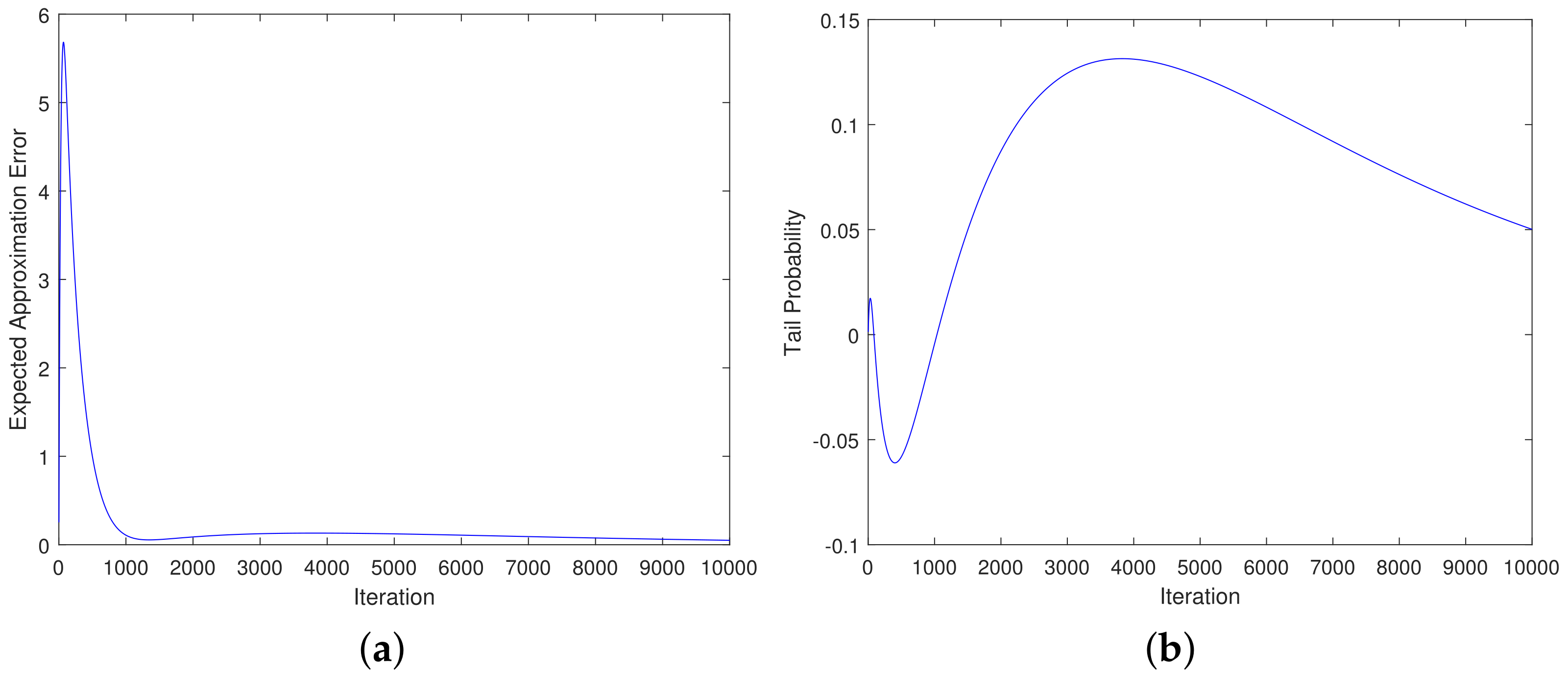
Example 4.

We construct two artificial Markov chains as the models of two EAs. Let $E{A}_{\mathcal{R}}$ and $E{A}_{\mathcal{S}}$ be two EAs starting with an identical initial distribution

$${\mathbf{p}}^{\left[0\right]}={\left(\frac{1}{n},\frac{1}{n},\cdots ,\frac{1}{n}\right)}^t,$$

and the respective transition matrices are

$$\begin{array}{c}\hfill \tilde{\mathbf{R}}=\left(\begin{array}{ccccc}1& \frac{1}{n^3}& \frac{2}{n^3}& \cdots & \frac{n}{n^3}\\ & 1-\frac{1}{n^3}& \frac{1}{n^2}& & \\ & & 1-\frac{1}{n^2}-\frac{2}{n^3}& \ddots & \\ & & & \ddots & \frac{n-1}{n^2}\\ & & & & 1-\frac{1}{n}\end{array}\right)\end{array}$$

and

$$\begin{array}{c}\hfill \tilde{\mathbf{S}}=\left(\begin{array}{ccccc}1& \frac{2}{n^3}& \frac{4}{n^3}& \cdots & \frac{2n}{n^3}\\ & 1-\frac{2}{n^3}& \frac{1}{n^2}+\frac{1}{2n}& & \\ & & 1-\frac{n^2+2n+8}{2n^3}& \ddots & \\ & & & \ddots & \frac{n-1}{n^2}+\frac{n-1}{2n}\\ & & & & 1-\frac{n^2+n+2}{2n^2}\end{array}\right).\end{array}$$

Obviously, it holds $\tilde{\mathbf{S}}⪰\tilde{\mathbf{R}}$. Through computer simulation, we get the curve of EAE difference of the two EAs in Figure 1a and the curve of TPs difference between the two EAs in Figure 1b. From Figure 1b, it is clear that $E{A}_{\mathcal{R}}$ does not always outperform $E{A}_{\mathcal{S}}$ because the difference of TPs is negative at the early stage of the iteration process but later positive.

Now we turn to discuss $(1+1)EA$ and $(1+1)E{A}_C$ on Deceptive. We demonstrate $(1+1)E{A}_C$ may not outperform $(1+1)EA$ over all generations although the transition matrix of $(1+1)E{A}_C$ dominates that of $(1+1)EA$.

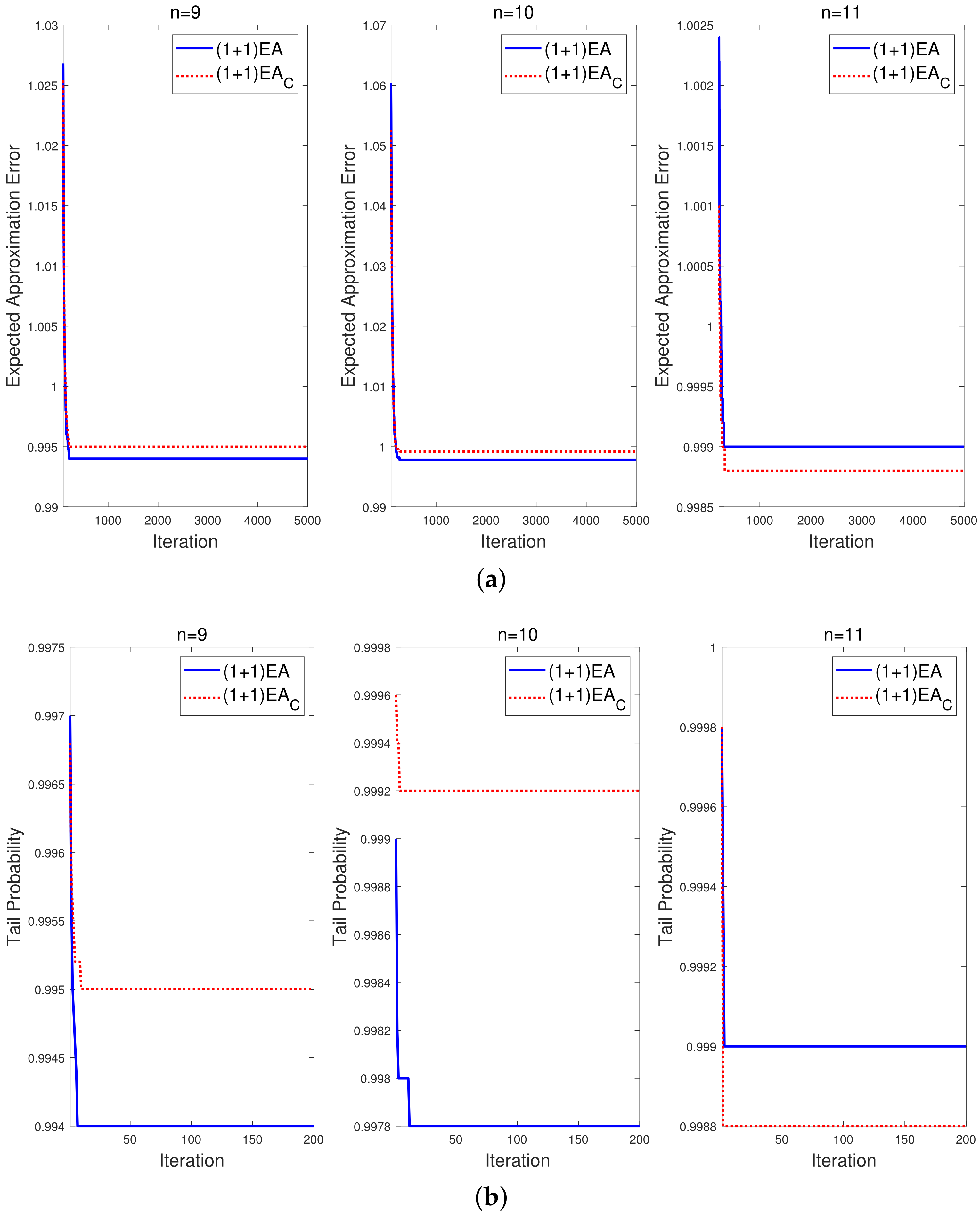
Example 5.

In $(1+1)EA$ and $(1+1)E{A}_C$, set $p_m=C_R{q}_m=1/n$. For $(1+1)E{A}_C$, let $q_m=\frac{1}{2}$, $C_R=\frac{2}{n}$. The numerical simulation results of EAEs and TPs for 5000 independent runs are depicted in Figure 2. It is shown that when $n\ge 9$, both EAEs and TPs of $(1+1)EA$ could be smaller than those of $(1+1)E{A}_C$. This indicates that the dominance of the transition matrix does not always guarantee the outperformance of the corresponding algorithm.

With $p_m=C_R{q}_m=p\le 1/n$, although the binomial crossover leads to transition dominance of $(1+1)E{A}_C$ over $(1+1)EA$, the enhancement of exploitation plays a governing role in the iteration process. Thus, the imbalance of exploration and exploitation leads to poor performance of $(1+1)E{A}_C$ at some stage of the iteration process. As shown in the previous two examples, the outperformance of $(1+1)E{A}_C$ cannot be drawn from the dominance of transition matrices.

The fitness landscape of Deceptive confirms that global convergence of EAs on Deceptive is principally attributed to the direct transition from level j to level 0, quantified by the transition probability $r_{0,j}$. By investigating the impact of binomial crossover on the transition probability $r_{0,j}$, we arrive at an adaptive strategy for the regulation of the mutation rate and the crossover rate, by which performance of both $(1+1)EA$ and $(1+1)E{A}_C$ are enhanced.

7.2. Comparisons on the Probabilities to Transfer from Non-Optimal Statuses to the Optimal Status

A comparison between $p_{0,j}$ and $s_{0,j}$ is performed by investigating their monotonicity. Substituting (13) and (14) into (23) and (24), respectively, we have

$$\begin{array}{cc}\hfill & p_{0,j}=P_1(n-j+1,p_m)={\left(p_m\right)}^{n-j+1}{(1-p_m)}^{j-1},\hfill \\ \hfill & s_{0,j}=P_3(n-j+1,C_R,q_m)\hfill \end{array}$$

(45)

$$\begin{array}{cc}\hfill & =\frac{1}{n}\left[(j-1)(1-C_R)+n{C}_R(1-q_m)\right]C_R^{n-j}{\left(q_m\right)}^{n-j+1}{\left(1-q_m{C}_R\right)}^{j-2}.\hfill \end{array}$$

(46)

We first investigate the maximum values of $p_{0,j}$ to get the ideal performance of $(1+1)EA$ on the Deceptive problem.

Theorem 5.

While

$$\begin{array}{cc}\hfill & p_m^{☆}=\frac{n-j+1}{n},\hfill \end{array}$$

(47)

$p_{0,j}$ gets its maximum values $p_{0,j}^{max}={\left(\frac{n-j+1}{n}\right)}^{n-j+1}{\left(\frac{j-1}{n}\right)}^{j-1}$.

Proof. 

By (45), we know

$$\begin{array}{c}\hfill \frac{\partial }{\partial p_m}{p}_{0,j}=(n-j+1-n{p}_m)p_m^{n-j}{\left(1-p_m\right)}^{j-2}.\end{array}$$

While $p_m=\frac{n-j+1}{n}$, $p_{0,j}$ gets its maximum value

$$p_{0,j}^{max}=P_1(n-j+1,\frac{n-j+1}{n})={\left(\frac{n-j+1}{n}\right)}^{n-j+1}{\left(\frac{j-1}{n}\right)}^{j-1}.$$

□

Influence of the binomial crossover on $s_{0,j}$ is investigated on condition that $p_m=q_m$. By regulating $C_R$, we compare $p_{0,j}$ with the maximum value $s_{0,j}^{max}$ of $s_{0,j}$.

Theorem 6.

On condition that $p_m=q_m$, the following results hold.

1.

$p_{0,1}=s_{0,1}^{max}$.

2.

If $q_m>\frac{n-1}{n}$, $p_{0,2}<s_{0,2}^{max}$; otherwise, $p_{0,2}=s_{0,2}^{max}$.

3.

$\forall j\in \{3,\cdots ,n-1\}$, $p_{0,j}\le s_{0,j}^{max}$ if $q_m>\frac{n-j}{n-1}$; otherwise, $s_{0,j}^{max}=p_{0,j}$.

4.

if $q_m>\frac{1}{n}$, $p_{0,n}<s_{0,n}^{max}$; otherwise, $s_{0,n}^{max}=p_{0,n}$.

Proof. 

Note that $(1+1)E{A}_C$ degrades to $(1+1)EA$ when $C_R=1$. Then, if the maximum value $s_{0,j}^{max}$ of $s_{0,j}$ is obtained by setting $C_R=1$, we have $s_{0,j}^{max}=p_{0,j}$; otherwise, it holds $s_{0,j}^{max}>p_{0,j}$.

(1)

For the case that $\mathbf{j}=\mathbf{1}$, Equation () implies

$$s_{0,1}=q_m^n{\left(C_R\right)}^{n-1}.$$

Obviously, $s_{0,1}$ is monotonously increasing in $C_R$. It gets the maximum value while $C_R^{☆}=1$. Then, by (45) we get $s_{0,1}^{max}=p_{0,1}$.

(2)

While $\mathbf{j}=\mathbf{2}$, by () we have

$$\frac{\partial s_{0,2}}{\partial C_R}=\frac{n-1}{n}{q}_m^{n-1}{\left(C_R\right)}^{n-3}\left(n-2+\left(1-n{q}_m\right)C_R\right).$$

• If $0<q_m\le \frac{n-1}{n}$, $s_{0,2}$ is monotonously increasing in $C_R$, and gets its maximum value while $C_R^{☆}=1$. For this case, we know $s_{0,2}^{max}=p_{0,2}$.
• While $\frac{n-1}{n}<q_m<1$, $s_{0,2}$ gets its maximum value $s_{0,2}^{max}$ by setting

  $$C_R^{☆}=\frac{n-2}{n{q}_m-1}.$$

  (48)
  Then, we have $s_{0,2}^{max}>p_{0,2}$.

(3)

For the case that $\mathbf{3}\le \mathbf{j}\le \mathbf{n}-\mathbf{1}$, we denote

$$s_{0,j}=\frac{n-j+1}{n}{q}_m^{n-j+1}{I}_1+\frac{\left(j-1\right)\left(1-q_m\right)}{n}{q}_m^{n-j+1}{I}_2,$$

where

$$\begin{array}{cc}\hfill & I_1={\left(C_R\right)}^{n-j}{\left(1-q_m{C}_R\right)}^{j-1},\hfill \\ \hfill & I_2={\left(C_R\right)}^{n-j+1}{\left(1-q_m{C}_R\right)}^{j-2}.\hfill \end{array}$$

Then,

$$\begin{array}{cc}\hfill & \frac{\partial I_1}{\partial C_R}={\left(C_R\right)}^{n-j-1}{\left(1-q_m{C}_R\right)}^{j-2}\left(n-j-\left(n-1\right)q_m{C}_R\right),\hfill \\ \hfill & \frac{\partial I_2}{\partial C_R}={\left(C_R\right)}^{n-j}{\left(1-\frac{C_R}{n}\right)}^{j-3}\left(n-j+1-\left(n-1\right)q_m{C}_R\right).\hfill \end{array}$$

• While $0<q_m\le \frac{n-j}{n-1}$, both $I_1$ and $I_2$ are increasing in $C_R$. For this case, $s_{0,j}$ gets its maximum value when $C_R^{☆}=1$, and we have $s_{0,j}^{max}=p_{0,j}$.
• If $\frac{n-j+1}{n-1}\le q_m\le 1$, $I_1$ gets its maximum value when $C_R=\frac{n-j}{(n-1)q_m}$, and $I_2$ gets its maximum value when $C_R=\frac{n-j+1}{(n-1)q_m}$. Then, $s_{0,j}$ get its maximum value $s_{0,j}^{max}$ at some

  $$C_R^{☆}\in \left(\frac{n-j}{(n-1)q_m},\frac{n-j+1}{(n-1)q_m}\right).$$

  (49)
  Accordingly, we know $s_{0,j}^{max}>p_{0,j}$.
• If $\frac{n-j}{n-1}<q_m<\frac{n-j+1}{n-1}$, $I_1$ gets its maximum value when $C_R=\frac{n-j}{(n-1)q_m}$, and $I_2$ is monotonously increasing in $C_R$. Then, $s_{0,j}$ get its maximum value $s_{0,j}^{max}$ at some

  $$C_R^{☆}\in \left(\frac{n-j}{(n-1)q_m},1\right],$$

  (50)

  and we know $s_{0,j}^{max}>p_{0,j}$.

(4)

While $\mathbf{j}=\mathbf{n}$, Equation () implies that

$$\begin{array}{c}\hfill \frac{\partial s_{0,n}}{\partial C_R}=\left(n-1\right){\left(1-q_m{C}_R\right)}^{n-3}\left(1-2q_m-\left(n-1-n{q}_m\right)q_m{C}_R\right).\end{array}$$

Denoting

$$g\left(q_m,C_R\right)=1-2q_m-\left(n-1-n{q}_m\right)q_m{C}_R,$$

we can confirm the sign of $\partial s_{0,n}/\partial C_R$ by considering

$$\frac{\partial }{\partial C_R}g\left(q_m,C_R\right)=-\left(n-1-n{q}_m\right)q_m.$$

• While $0<q_m\le \frac{n-1}{n}$, $g\left(q_m,C_R\right)$ is monotonously decreasing in $C_R$, and its minimum value is

  $$g\left(q_m,1\right)=\left(n{q}_m-1\right)\left(q_m-1\right).$$
  The maximum value of $g\left(q_m,C_R\right)$ is

  $$g\left(q_m,0\right)=1-2q_m.$$

  (a)

  If $0<q_m\le \frac{1}{n}$, we have

  $$g\left(q_m,C_R\right)\ge g\left(q_m,1\right)>0.$$

  Thus, $\frac{\partial s_{0,n}}{\partial C_R}\ge 0$, and $s_{0,n}$ is increasing in $C_R$. For this case, $s_{0,n}$ get its maximum value when $C_R^{☆}=1$, and we have $s_{0,n}^{max}=p_{0,n}$.

  (b)

  If $\frac{1}{n}<q_m\le \frac{1}{2}$, $s_{0,n}$ gets the maximum value $s_{0,n}^{max}$ when

  $$C_R^{☆}=\frac{1-2q_m}{q_m(n-1-n{q}_m)}.$$

  Thus, $s_{0,n}^{max}>p_{0,n}$.

  (c)

  If $\frac{1}{2}<q_m\le \frac{n-1}{n}$, $g\left(q_m,0\right)<0$, and then, $s_{0,n}$ is decreasing in $C_R$. Then, its maximum value is obtained by setting $C_R^{☆}=0$, and we know $s_{0,n}^{max}>p_{0,n}$.

• While $\frac{n-1}{n}<q_m\le 1$, $g\left(q_m,C_R\right)$ is increasing in $C_R$, and its maximum value is

  $$g\left(q_m,1\right)=\left(n{q}_m-1\right)\left(q_m-1\right)<0.$$
  Then, $s_{0,n}$ is monotonously decreasing in $C_R$, and its maximum value is obtained by setting $C_R^{☆}=0$. Accordingly, we know $s_{0,n}^{max}>p_{0,n}$.

In summary, $s_{0,n}^{max}>p_{0,n}$ while $q_m>\frac{1}{n}$; otherwise, $s_{0,n}^{max}=p_{0,n}$.

□

Theorems 5 and 6 present the “best” settings to maximize the transition probabilities from non-optimal statuses to the optimal level, by which we get a parameter adaptive strategy that greatly enhances the exploration of compared EAs.

7.3. Parameter Adaptive Strategy to Enhance Exploration of EAs

Since the level index j is equal to the Hamming distance between $\mathbf{x}$ and ${\mathbf{x}}^{*}$, improvement of level index j is bounded by reduction of the Hamming distance obtained by replacing $\mathbf{x}$ with $\mathbf{y}$. Then, while the local exploitation leads to a transition from level j to a non-optimal level i, the practically adaptive strategy of parameters can be obtained according to the Hamming distance between $\mathbf{x}$ and $\mathbf{y}$.

When $(1+1)EA$ is located at the solution $\mathbf{x}$ at status j, Equation (47) implies that the “best” setting of mutation rate is $p_m^{☆}\left(j\right)=\frac{n-j+1}{n}$. Once it transfers to solution $\mathbf{y}$ at status $i(i<j)$, the “best” setting changes to $p_m^{☆}\left(i\right)=\frac{n-i+1}{n}$. Then, the difference of “best” settings is $\frac{j-i}{n}$, bounded from above by $\frac{H(\mathbf{x},\mathbf{y})}{n}$. Accordingly, the mutation rate of $(1+1)EA$ can be updated to

$$p_m^{\prime }=p_m+\frac{H(\mathbf{x},\mathbf{y})}{n}.$$

(51)

For $(1+1)E{A}_C$, the parameter $q_m$ is adapted using the strategy consistent to that of $p_m$ to focus on influence of $C_R$. That is,

$$q_m^{\prime }=q_m+\frac{H(\mathbf{x},\mathbf{y})}{n}.$$

(52)

Since $s_{0,j}$ demonstrates different monotonicity for varied levels, one cannot get an identical strategy for the adaptive setting of $C_R$. As a compromise, we would like to consider the case that $3\le j\le n-1$, which is obtained by random initialization with overwhelming probability.

According to the proof of Theorem 6, we know $C_R$ should be set as great as possible for the case $q_m\in (0,\frac{n-j}{n-1}]$; while $q_m\in (\frac{n-j}{n-1},1]$, $C_R^{☆}$ is located in intervals whose boundary values are $\frac{n-j}{(n-1)q_m}$ and $\frac{n-j+1}{(n-1)q_m}$, given by (49) and (50), respectively. Then, while $q_m$ is updated by (52), the update strategy of $C_R$ can be confirmed to satisfy that

$$C_R^{\prime }{q}_m^{\prime }=C_R{q}_m+\frac{H(\mathbf{x},\mathbf{y})}{n-1}.$$

Accordingly, the adaptive setting of $C_R$ could be

$$C_R^{\prime }=\left(C_R{q}_m+\frac{H(\mathbf{x},\mathbf{y})}{n-1}\right)/q_m^{\prime },$$

(53)

where $q_m^{\prime }$ is updated by (52).

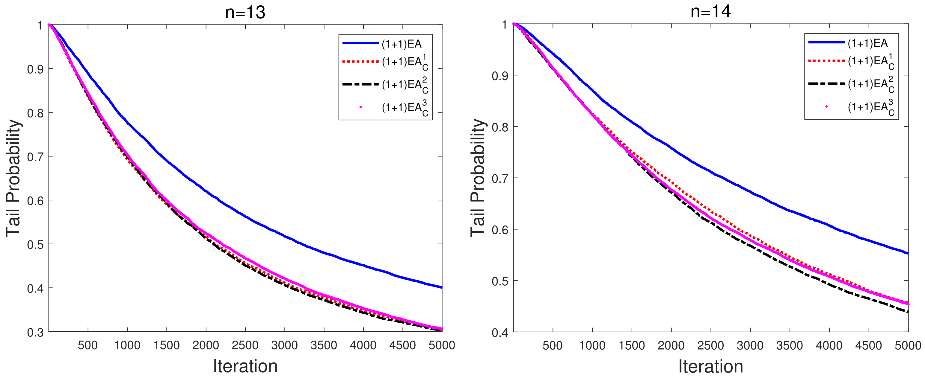
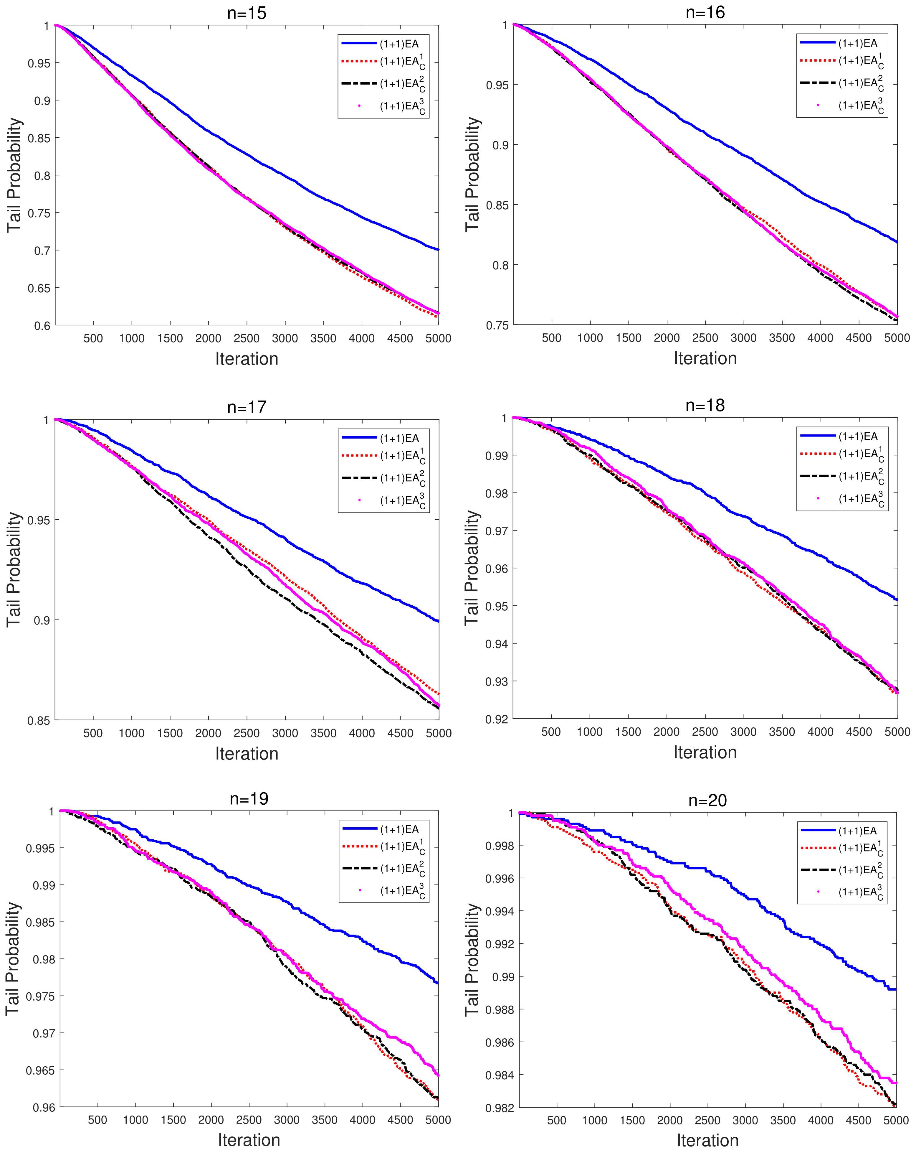
By incorporating the adaptive strategy (51) to $(1+1)EA$, we compare the performance of its adaptive variant with the adaptive $(1+1)E{A}_C$ that regulates its mutation rate and crossover rate by (52) and (53), respectively. For 13–20 dimensional Deceptive problems, numerical simulation of the tail probability is implemented by 10,000 independent runs. The initial value of $p_m$ is set as $\frac{1}{n}$. To investigate the sensitivity of the adaptive strategy on initial values of $q_m$, the mutation rate $q_m$ in $(1+1)E{A}_C$ is initialized with values $\frac{1}{\sqrt{n}}$, $\frac{3}{2\sqrt{n}}$ and $\frac{2}{\sqrt{n}}$, and the corresponding variants are denoted by $(1+1)E{A}_C^1$, $(1+1)E{A}_C^2$ and $(1+1)E{A}_C^3$, respectively.

The converging curves of averaged TPs are illustrated in Figure 3. Compared to the EAs with fixed parameters during the evolution process, the performance of the adaptive EAs on Deceptive has been significantly improved. Furthermore, we also note that the converging curves of adaptive $(1+1)E{A}_C$ are not sensitive to the initial mutation rate. Although transition dominance does not necessarily lead to outperformance of $(1+1)E{A}_C$ over $(1+1)EA$, the proposed adaptive strategy can greatly enhance global exploration of $(1+1)E{A}_C$ to a large extent, and consequently, we get the improved adaptive $(1+1)E{A}_C$ that is not sensitive to initial mutation rates.

8. Conclusions and Discussions

Under the framework of fixed-budget analysis, we conduct a pioneering analysis of the influence of binomial crossover on the approximation error of EAs. The performance of EAs after running finite generations is measured by two metrics: the expected value of the approximation error and the error tail probability, by which we make a case study by comparing the performance of $(1+1)EA$ and $(1+1)E{A}_C$ with binomial crossover.

Starting from the comparison of the probability of flipping “l preferred bits”, it is proven that under proper conditions, incorporation of binomial crossover leads to the dominance of transition probabilities, that is, the probability of transferring to any promising status is improved. Accordingly, the asymptotic performance of $(1+1)E{A}_C$ is superior to that of $(1+1)EA$.

It is found that the dominance of transition probability guarantees that $(1+1)E{A}_C$ outperforms $(1+1)EA$ on OneMax in terms of both expected approximation error and tail probability. However, this dominance does lead to the outperformance on Deceptive. This means that using binomial crossover may improve the performance on some problems but not on other problems.

For Deceptive, an adaptive strategy of parameter setting is proposed based on the monotonicity analysis of transition probabilities. Numerical simulations demonstrate that it can significantly improve the exploration ability of both $(1+1)E{A}_C$ and $(1+1)EA$, and superiority of binomial crossover is further strengthened by the adaptive strategy. Thus, a problem-specific adaptive strategy is helpful for improving the performance of EAs.

Our future work will focus on a further study for the adaptive setting of crossover rate in population-based EAs on more complex problems, as well as the development of adaptive EAs improved by the introduction of binomial crossover.