Article

Nonlinear Mixed Convection in a Reactive Third-Grade Fluid Flow with Convective Wall Cooling and Variable Properties

by
Samuel Olumide Adesanya
1,*,
Tunde Abdulkadir Yusuf
2 and
Ramoshweu Solomon Lebelo
3
1
Department of Mathematics and Statistics, Faculty of Natural Sciences, Redeemer’s University, Ede 232101, Nigeria
2
Department of Mathematics, Faculty of Science, Adeleke University, Ede 232104, Nigeria
3
Education Department, Vaal University of Technology, Private Bag X021, Vanderbijlpark 1911, South Africa
*
Author to whom correspondence should be addressed.
Mathematics 2022, 10(22), 4276; https://doi.org/10.3390/math10224276
Submission received: 6 October 2022 / Revised: 2 November 2022 / Accepted: 9 November 2022 / Published: 15 November 2022
(This article belongs to the Special Issue Analysis and Applications of Mathematical Fluid Dynamics)

Abstract

:
Energy management and heat control whenever a reactive viscous fluid is the working medium has been one of the greatest challenges encountered by many in the field of chemical and industrial engineering. A mathematical approach to thedetermination of critical points beyond which the working environment becomes hazardous is presented in the present investigation together with the entropy generation analysis that guarantees the efficient management of expensive energy resources. In this regard, the nonlinear mixed convective flow behavior of a combustible third-grade fluid through a vertical channel with wall cooling by convection is investigated. The mathematical formulation captures the nonlinearities arising from second-order Boussinesq approximation and exponential dependence of internal heat generation, viscosity, and thermal conductivity on temperature. The resulting nonlinear boundary value problems were solved based on the spectral Chebyshev collocation method (SCCM) and validated with the shooting-Runge–Kutta method (RK4). The nonlinear effects on the flow velocity, temperature distribution, entropy generation, and Bejan heat irreversibility ratio are significant. Further analyses include the thermal stability of the fluid. Findings from the study revealed that flow, temperature, and entropy generation are enhanced byincreasing values of the Grashof number, the quadratic component of buoyancy, and the Frank-Kameneskii parameter, but are reducedbyincreasing the third-grade material parameter. Moreover, it was shown that increasing values of the third-grade parameter encourages the thermal stability of the flow, while increasing values of the linear and nonlinear buoyancy parameter destabilizes the flow. The present result is applicable to thick combustible polymers with increased molecular weight.

1. Introduction

A renewed interest in energy utilization and management has led to a significant increase in studies centered on a broad range of reactive non-Newtonian fluids in the last few decades. A good number of researchers gave mathematical explanations from a fluid dynamics viewpoint on how best to maximize exergy when working with reactive fluids. For instance, Salawu et al. [1] reported the transient flow of a reactive fourth-order fluid through a horizontal channel
Permeated by a magnetic field, Cuiet al.in [2] investigated the two-dimensional reacting flow of hydromagnetic nano-Oldroyd-B fluid driven by mixed convection. In [3], Salawu and his cohorts considered the slip flow of combustible MHD couple stress fluids with variable properties. Sadiq and Hayat [4] presented a model for optimizing entropy generation in Reiner–Rivlin flow over a stretched rotating disc. Okoya [5] reported a numerical investigation of a time-independent variable viscous third-grade fluid flow through a cylinder. Adesanya et al. [6] analyzed the flow of third-grade fluid between two solid boundaries under Arrhenius kinetics. The study in [7] focused on the reactive flow under the Erying–Powell constitutive model. More studies on reactive flows of third-grade fluid can be found in [8,9,10,11,12,13,14] and the literature cited therein.
The quantity of energy absorbed by the flow is defined by the degree of friction caused by viscosity, which plays a crucial role in the creation of fluid measures for flow measurements. The changing viscosity in Couette and Poiseuille flows of a tangential hyperbolic fluid via an inclined channel with porous media was explored by Zehra et al. [15]. The fluid’s viscosity has been assumed in this research to be inversely proportional to a linear function of pressure. It should go without saying that the viscosity and thermal conductivity of any fluid may be alteredas the temperature rises. This phenomenon therefore plays a crucial role in the rate of heat transport near the surface, much as other thermophysical features. It is acknowledged that certain characteristics, particularly fluid viscosity, may vary with temperature. This change in viscosity and thermal conductivity must be taken into consideration in order to correctly forecast the flow and heat transfer rates. Jeffrey fluid flow, heat transfer, and mass transfer via a permeable wave-like channel with variable viscosity and thermal conductivity were studied by Manjunatha et al. in their study [16]. Qasim et al.’s [17] investigation on the impact of dissipation of a fluid flow through a tiny needle takes these fluid parameters into account. Recently, Saraswathy et al. [18] investigated these phenomena in order to use a numerical approach to investigate the solution for an asymmetric flow and heat transfer of a rotating fluid with the influence of Arrhenius energy.
Additionally, while the first law of thermodynamics has been used by certain writers, its efficacy has been shown to be inferior to that of the second law. Thermal efficiency decreases and system entropy increases as a result of energy losses in engineering and thermal equipment. It is well known that the development of entropy during any thermal process determines the degree of irreversibility. The optimization procedures have recently paid a lot of attention to this examination. Many thermal systems may include irreversible processes. The second law of thermodynamics has been extensively employed in the literature to enhance these types of irreversibility. In this light, Khan et al. [19] analyzed the formation of entropy on an Erying–Powell liquid flowing via a permeable channel using a homotopy analysis technique. Singh et al. [20] investigated the entropy generation impact in a micropolar fluid flowing through an aligned tube. Here, it is claimed that the fluid’s viscosity and thermal conductivity both change with temperature. The conclusion of their analysis shows that temperature-dependent thermal and viscous conductivity factors enhance the entropy production profile. Similar studies on entropy production rates and irreversibility in convection-based heat transport may be found in references [21,22,23].
In modeling the flow driving mechanism, the nonlinear temperature-density relationship has been established over the years to give a better approximation than the linearized form of heat transfer in a wide range of buoyancy-driven flows due to the considerable difference in the fluid temperature and the ambient. Given these numerous applications, Adesanyaet al. [24] focused on the entropy generation, flow, and nonlinear heat transfer to a couple stress fluid flow through aporous medium. In the Xiaet al. [25] report, a mathematical explanation for the nonlinear bio-convective flow of hydromagnetic fluid containing microorganisms with Hall effect is discussed. Ibrahim and Gadisa [26] presented a finite element residual approximation for Oldroyd-B flow with internal heat generation. Patilet al. [27] constructed the numerical approximation to nonlinear convective flow problems with Brownian and thermophoresis. Waqaset al. [28] reported the steady developing flow of Williamson fluid with variable diffusion and thermal conductivity. A semi-analytical approach is employed by Yusuf et al. [29] to examine the magnetohydrodynamic (MHD) nonlinear convective flow of a reactive non-Newtonian fluid model with convective heating. Other vital studies on nonlinear convective flows include refs. [30,31,32] and the cited references.
Despite the huge body of literature surrounding heat irreversibility in a combustible non-Newtonian fluid flow, the nonlineardependence of some fluid parameters on temperatureremains poorly understood with respect to thermal stability for the determination of safe working conditions and energy management or efficiency. The proposed nonlinear coupled model will ensure that the thermal system is not underdetermined when used to predict buoyancy-induced flow and thermal behavior. The nonlinearity of the model suggests the non-existence of a close-form solution; therefore, the present work focuses on a fast-converging numerical approach totackling the coupled nonlinear convective flow and heat transfer problem. To the best of our knowledge, the problem presented here has not been undertaken byany researcher, and that explains the novelty of the work.
Including the nonlinear buoyancy approximation, nonlinear internal heat, and exponential dependence of fluid viscosity and thermal conductivity is expected to produce a better approximation of reactive flow and heat transfer problems, especially during a number of engineering processes, such as advanced powder synthesis by self-propagating high-temperature, heat exchangers, loop/fluidized bed reactors, treatment of reactive hydrocarbons, combustion chambers and many more engineering applications. In the next section, the mathematical analysis of the problem is presented.

2. Mathematical Formulation

In the model formulation, we consider a fully-developed flow of a reactive third-grade fluid flow through a vertical channel with Newtonian cooling at the walls. The buoyancy effect is felt upstream in the vertical x-axis while the y-axis is perpendicular to it, as shown in Figure 1. All the fluid properties like viscosity, thermal conductivity, and internal heat generation are assumed to vary with temperature in an exponential manner, except density which has quadratic dependence.
Under the flow assumptions, the vector form for the momentum equation becomes:
ρ D V D t = ρ g + d i v τ
where the operator, D ( . ) D t = ( t + V . ) ( . ) is the material derivate acting on the velocity vector V , and ρ , g -density and gravitational force, respectively. The last term τ is the Cauchy stress tensor defined as [14,33]
τ = P I + μ S 1 + α 1 S 2 + α 2 S 1 2 + β 1 S 3 + β 2 ( S 1 S 2 + S 2 S 1 ) + β 3 ( t r S 1 2 ) S 1
In (2), α n ,   ( n = 1 , 2 , 3 ) , β n ,   ( n = 1 , 2 , 3 ) are material effects, ( P , I , μ ) are the pressure, tensor identity and fluid viscosity, respectively while S n ,   ( n = 1 , 2 , 3 ) represents the Rilvin–Ericksen tensors and are defined as
S 1 = V + ( V ) T S n = D S n 1 D t + S n 1 V + ( V ) T S n 1 ,       n > 1
The Clausius–Duhem inequality condition μ 0 ,   α 1 0   , | α 1 + α 2 | 24 μ β 3 ensures the thermodynamic process is consistent when β 1 = β 2 = 0 implies that β 3 0 .
Therefore, (2) reduces to
τ = P I + ( μ + β 3 ( t r S 1 2 ) ) S 1 + α 1 S 2 + α 2 S 1 2
From (4), it is easy to note that the effective viscosity, which is assumed to be a nonlinear function of temperature, becomes
μ e f f = μ ( T ) + β 3 ( t r S 1 2 )
As a consequence of (5), the momentum equation with the nonlinear temperature-dependent fluid density becomes
0 = d P d x + d d y ( μ ( T ) d u d y + 2 β 3 ( d u d y ) 3 )   + ρ g ϕ 0 ( T T 0 ) + ρ g ϕ 1 ( T T 0 ) 2
While the balanced energy equation with variability in thermal conductivity becomes
0 = d d y ( k ( T ) d T d y ) + Q C 0 A ( h T υ l ) m e E R T   + ( μ ( T ) + 2 β 3 ( d u d y ) 2 ) ( d u d y ) 2
The fact that the heat transfer to the viscous non-Newtonian fluid is irreversible suggests that the entropy generation profile is a nonlinear combination of heat transfer and fluid friction, that is,
E G = k ( T ) T 0 2 ( d T d y ) 2 + 1 T 0 ( d u d y ) 2 ( μ ( T ) + 2 β 3 ( d u d y ) 2 )
Togetherwith the essential and temperature dependent natural boundary conditions
u = 0 ,     k ( T ) d T d y = h 1 ( T 0 T )                               y = 0 u = 0 ,     k ( T ) d T d y = h 2 ( T T 0 )                               y = a
Of engineering interest is the wall skin friction and Nusselt number for heat transfer at the wall
C f = μ 0 e α ¯ ( T T 0 ) d u d y + 2 β 3   ( d u d y ) 3 | y = 0 ,       q w =   k 0 e η ¯ ( T T 0 ) d T d y | y = 0
The Reynold’s exponential dependence of viscosity and thermal conductivity on temperature is assumed to take the form
μ ( T ) = μ 0 e α ¯ ( T T 0 ) ,   k ( T ) = k 0 e η ¯ ( T T 0 )
With the introduction of the following variables and parameters
y = y a ,           u = u U G ,             θ = E ( T T 0 ) R T 0 2 , α = α ¯ R T 0 2 E , γ = β 3 U 2 G 2 μ 0 a 2 , δ = ( υ ι T 0 ) m μ 0 U 2 G 2 Q A C 0 a 2 e E R T 0 G = a 2 μ 0 U G d P d x = 1 , G r = ρ g ϕ 0 a 2 R T 0 2 μ 0 E U G , σ = ϕ 1 R T 0 2 ϕ 0 E , λ = ( T 0 υ ι ) m Q E A a 2 C 0 k 0 R T 0 2 e E R T 0 , B i 1 , 2 = h 1 , 2 a k 0 }
We obtainthe following dimensionless, nonlinear, coupled, system of boundary value problems
0 = 1 + d d y ( e α θ d u d y ) + 6 γ ( d u d y ) 2 d 2 u d y 2 + G r ( θ + σ θ 2 ) ,     u ( 0 ) = 0 = u ( 1 ) ; 0 = d d y ( e η θ d θ d y ) + λ ( ( 1 + ε θ ) m e θ 1 + ε θ + δ ( d u d y ) 2 ( e α θ + 2 γ ( d u d y ) 2 ) ) ,                                           ( e η θ d θ d y B i 1 θ ) | y = 0   = 0   = ( e η θ d θ d y + B i 2 θ ) | y = 1 .   }
Please note that the special case of the coupled Equation (13) is the non-reactive Newtonian flow when α = γ = G r = η = 0 , that was reported numerically in [33] by using shooting-Runge–Kutta scheme within Maple environment. In its dimensionless form, the expression for the positive definite entropy generation becomes
N S =   e η θ ( d θ d y ) 2 N h + λ δ ε ( ( d u d y ) 2 ( e α θ + 2 γ ( d u d y ) 2 ) ) N f
Component-wise, the Bejan irreversibility ratio becomes
B e = N h N s = N h N h + N f
While the expressions for the dimensionless skin friction and Nusselt number becomes
S f = ρ a 2 C f μ 0 2 = e α θ d u d y + 2 γ   ( d u d y ) 3 | y = 0 ,     N u = a E q w k 0 R T 0 2 =   e η θ d θ d y | y = 0

3. Solution by Weighted Residual Method

A collocation method based on Chebyshev polynomials is considered here to obtain numerical solutions of a differential equationin [0, L]. This technique approximatesa solution to a differential equation
f ( ϕ ( x ) ) + g ( x ) = 0 ,   in   domain ,   D = [ 0 , L ]
The approximate solution needs to satisfy the boundary conditions and it is given as
ψ ( x ) = i = 0 N k i T i ( 2 x L 1 )
where ϕ ( x ) is the unknown dependent function, f(x) is the source term, k i are undetermined coefficients, T i ( 2 x L 1 ) are shifted Chebyshev base functions from [−1,1] to [0, L]. To acquire the values of k i , Equation (18) is inserted into Equation (17) to yield residual error R ψ ( x , k i ) . R ψ ( x , k i ) is forced to be closer to zero using the collocation method as follows;
for   δ ( x x j ) = { 1 , x = x j 0 , otherwise ,
0 1 R ψ ( x , k i ) δ ( x x j ) d x = R ψ ( x , k i ) = 0 ,       for   j = 1 ,   2 , N 1
where x j = 1 2 ( 1 cos ( j π N ) ) are shifted Gauss–Lobatto points. Therefore, Equation (14) as well as the equations generated from the boundary conditions constitute a system of algebraic equations that must be solved in order to obtainthe constant coeficient values, k i . In order to obtain the solutions of Equation (13), solutions are assumed for u ( y ) and θ ( y ) , respectively, in the form:
u ( y ) = i = 0 N a i T i ( 2 y 1 ) ,             θ ( y ) = i = 0 N b i T i ( 2 y 1 )
where a i and b i are constants to be determined, and T i ( 2 y 1 ) are the shifted Chebyshev base functions. To obtain the values of a i and b i , to satisfy the boundary conditions, Equation (20) is substituted into the boundary conditions in Equation (13) and thus have
i = 0 N T a i ( 2 y 1 ) | y = 0 = 0 = i = 0 N T a i ( 2 y 1 ) | y = 1 ,
e η ( i = 0 N T b i ( 2 y 1 ) ) i = 0 N d T i d y b i ( 2 y 1 ) B i 1 i = 0 N T b i ( 2 y 1 ) | y = 0 = 0 = e η ( i = 0 N T b i ( 2 y 1 ) ) i = 0 N d T i d y b i ( 2 y 1 ) B i 2 i = 0 N T b i ( 2 y 1 ) | y = 1
Equation (15) is also substituted into Equations (9) and (10), resulting in r e s u ( y , a i ) and r e s θ ( y , a i , b i ) , respectively, as residues. At this juncture, the residues are forced to be zero by applying collocation method as follows
0 1 r e s u δ ( y y j ) d y = r e s u ( y j , a i ) = 0 ,   for   j = 1 , 2 , N 1 0 1 r e s θ δ ( y y j ) d y = r e s θ ( y j , a i , b i ) = 0 ,       for   j = 1 , 2 , N 1
where y j = 1 2 ( 1 cos ( j π N ) ) . Thus, Equations (16)–(18) form 2N + 2 system of algebraic equations containing 2N + 2 undetermined coefficients ( a i , b i ) . This procdeure is coded in a mathematicalsymbolic software to solve the generated equations using the Newton technique.

4. Solution by Shooting-Runge–Kutta Method

To achieve a numerical solution by the Runge–Kutta scheme, we first apply the shooting technique to the coupled problem by converting the second-order differential equations to a set of first-order ordinary Lipshitz continuous differential equations.
z 1 = u ,   z 2 = u ,   z 3 = θ ,   z 4 = θ
With (8), the coupled BVP becomes a coupled system of first order differential equations
( z 1 z 2 z 3 z 4 ) = ( z 2 α e α z 3 G r ( z 3 + σ z 3 2 ) 1 e α z 3 + 6 γ z 2 2 z 4 e η z 3 ( η e η z 3 z 4 2 λ { ( 1 + ε z 3 ) m e z 3 1 + ε z 3 + δ z 2 2 ( e α z 3 + 2 γ e α z 3 ) } ) )    
with the set of initial conditions
( z 1 ( 0 ) z 2 ( 0 ) z 3 ( 0 ) z 4 ( 0 ) ) = ( 0 D 1 z 4 ( 0 ) e η z 3 B i 1 D 2 )
Since the derivatives are not specified at the initial point, D 1 , 2 are therefore given initial guess values that ensure the boundary conditions are okay at the wall y = 1. It is easy to see that the sufficient condition that confirms the existence of a unique solution to the system of Equations (24) and (25)is satisfied as long as the Lipchitz constant f i x j K is bounded. The first-order equations are then carefully coded and solved by Runge–Kutta using the Mathematica package.

5. Results and Discussion

In this section, a physical interpretation of the numerical results is presented and discussed as regards the flow and thermal behavior. Table 1 and Table 2 represent the validation of the point collocation weighted residual method with the shooting-Runge–Kutta procedure for the dimensionless momentum and energy equations. A good agreement is observed between the two computations. This confirmed the uniqueness of the numerical solutions. Table 3 shows the convergence of the of the spectral collocation solution. The convergence of the solution to the highly nonlinear boundary value problem is seen to improve with an increasing number of terms N used in the approximation. Table 4 represents the computational result of the thermal stability analysis of the fluid. As observed from the plot, an increase in the nonlinear component of the Grashof number is seen to destabilize the flow thermal structure due increasing buoyancy force over viscous forces in the flow field. Additionally, an increase in the viscosity variation parameter is also observed to have a destabilizing effect on the fluid flow. This is true, since viscosity is expected to drop and fluid experiences shear thinning, which aids heat generation by kinetic theory of matter. Moreover, a rise in the third-grade parameter is seen to enhance thermal stability due to the thickening effect of the fluid. The thermal conductivity variation parameter increase is seen to discourage the thermal stability of the fluid flow. A similar behavior is seen with increasing values of the Grashof number due to increasing buoyancy forces. Table 5 and Table 6 revealed the accuracy of the solution when compared with already-published results in the special case when the fluid is Newtonian, non-reactive, with constant physical properties.
Figure 2 represents the variation of third-grade material effect with velocity, temperature, entropy generation, and Bejan number, as shown in Figure 2a–d, respectively. The thickening effect is manifested in Figure 2a as the third-grade material parameter grows. Likewise in Figure 2b, thickening of the fluid is seen to make the non-Newtonian fluid colder. This is physically correct because the kinetic energy of the flow decreases as a result, the intermolecular bond is expected to increase. Therefore, the activation energy requirement will be much higher to induce chemical reaction. The result from Figure 2c reveals that as the third-grade material parameter rises, there is drop in the entropy generation at the cooled walls. This is reasonable, because a rise in the third-grade material parameter has been shown to reduce the flow velocity and temperature maximum in Figure 2a,b. Therefore, available energy for work is maximum with the thickened fluid. Finally, in Figure 2d the result of the heat irreversibility ratio credited Bejan is presented. If we suppose that the fluid velocity and density are both constant, then we have a case of slab with Be = 1. However, for a variable viscous third-grade flow, we have seen that velocity is a decreasing function of the third-grade parameter. As a result, the kinetic energy of the flow drops with increasing value of the parameter. Therefore, heat transfer irreversibility is expected to gain dominance over frictional irreversibility as shown in the plot.
Figure 3a–d represent the impact of buoyancy forces on the flow field on the velocity, temperature, entropy generation rate, and the Bejan number respectively. From Figure 3a, the velocity profile shows that when Gr = 1 implies a simple case when viscous force and buoyancy force are equal. Further increase in the Grashof number implies that the contribution of viscous force is weaker when compared with buoyancy, therefore, the flow velocity increases significantly in response to the nonlinear buoyancy forces. A similar behavior is seen in the profile for fluid temperature (see Figure 3b) resulting from increase in the kinetic energy of the fluid. Consequently in Figure 3c, the entropy profile is expected to increase due to increase in both flow and temperature maximum. In Figure 3d, rise in Grashof number implies increasing temperature as seen in Figure 3b. Therefore, increasing temperature translates to a decreased rate of heat transfer, this shows that irreversibility due to frictional interactions is more when compared with heat transfer irreversibility as revealed in Figure 3d. The graphical representations of the effect of the nonlinear convection component of the Grashof number on the flow velocity, temperature, entropy generation, and Bejan number respectively depicted in Figure 4a–d. The point when σ = 0 corresponds to the linearized buoyancy parameter when the nonlinear effect is neglected. As shown in the Figure 4a, this parameter has a significant effect on the fluid flow and cannot be neglected. Also, in Figure 4b, an increased value of the parameter is also seen to elevate the fluid temperature maximum. Similar effect is noticed in Figure 4c, the rate of entropy generation improves at both convective walls while in Figure 4d, the frictional irreversibility decreases within the flow channel, due to a decrease in heat transfer.
The influence of the reaction kinetics coefficient ( λ ) on the flow and thermal structure is presented in Figure 5a. It is evidently shown that the velocity distribution enhanced for larger λ . This is due to the thinning effect on the fluid viscosity and the heat transfer from the strongly exothermic reaction to the fluid. In Figure 5b, similar behavior is experienced with the fluid temperature, except at the cooled walls with increasing flow and temperature. As expected the entropy generation rate is to rise for increased values of λ as shown in Figure 5c, while larger λ significantly increase the Bejan profile. This in turn encourages heat transfer irreversibility over fluid friction irreversibility as seen in Figure 5d.
Finally, Figure 6a–c shows the bifurcation plots for different reaction kinetics (m = −2, 0, 0.5). As observed from these plots, the blow-up point increases with increasing values of the exponent, thus thermal stability is enhanced.

6. Concluding Remarks

In this study, a time-independent flow and heat transfer of reactive third-order fluid has been investigated numerically, taking dependence of some physical properties on temperature into consideration. The nonlinear equations were solved numerically by using a spectral Chebyshev weighted residual method and validated by shooting-Runge–Kutta approach. The main contributions to knowledge from the study are listed as follows:
-
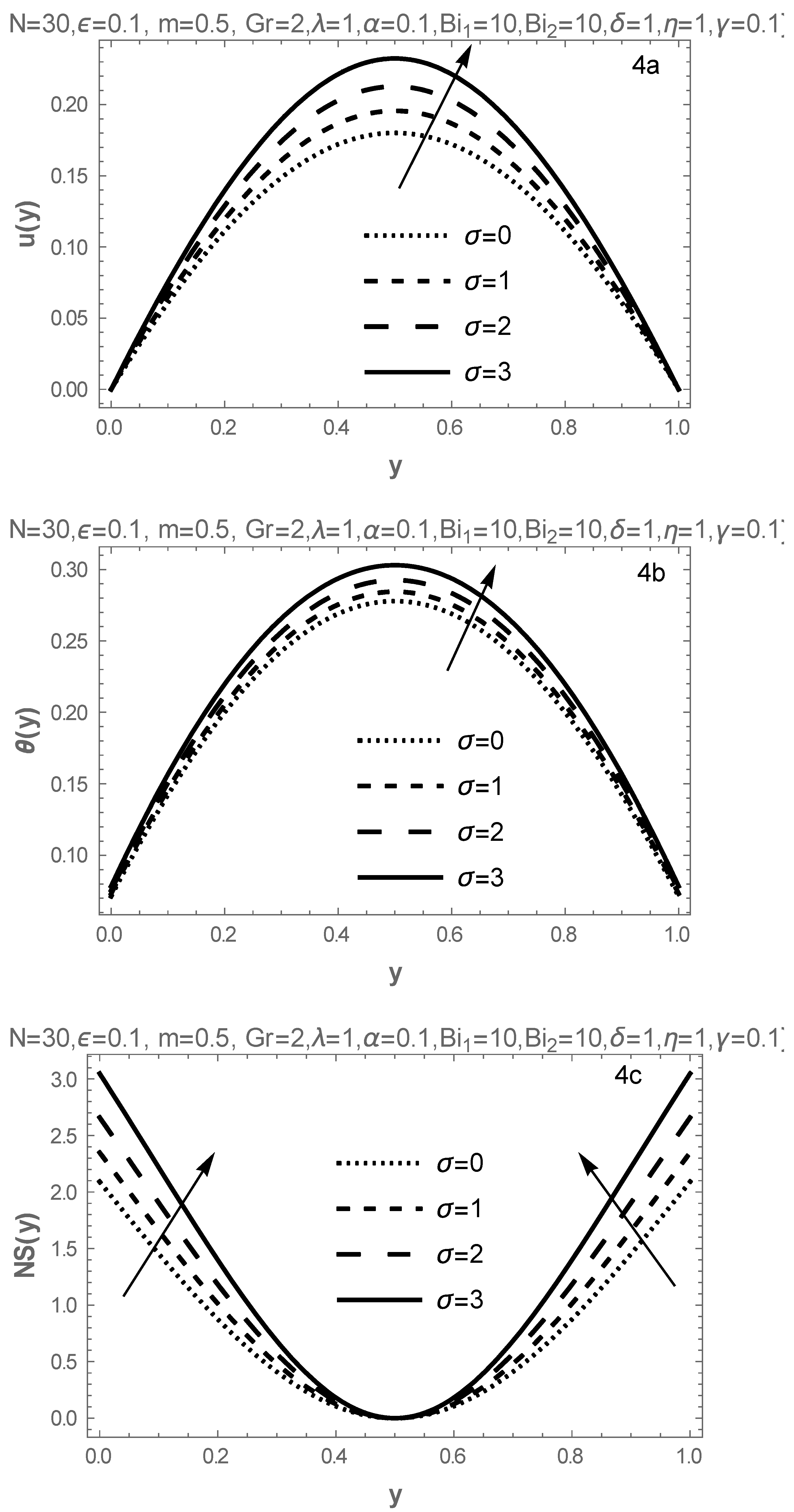
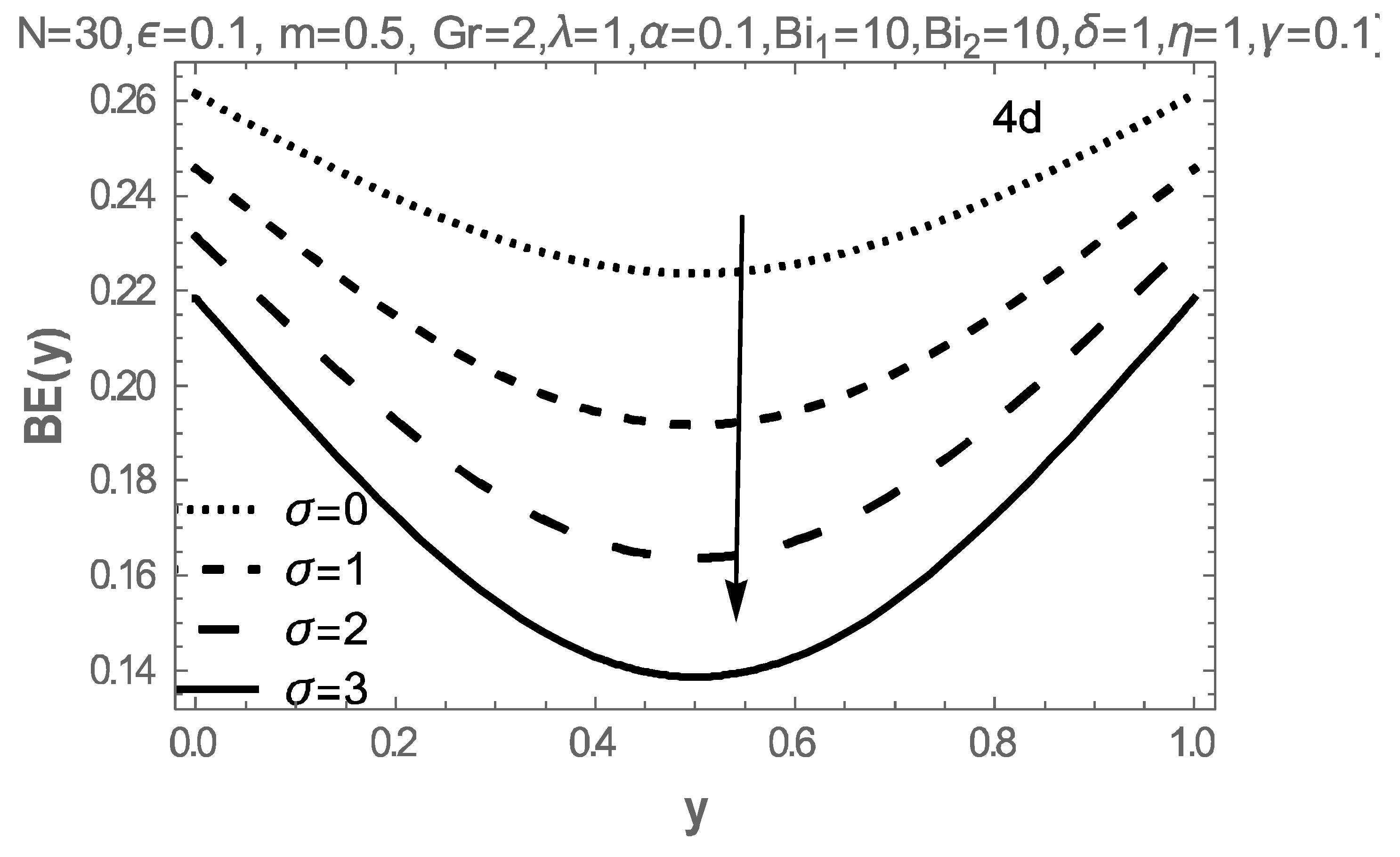
Flow, temperature, and entropy generation are enhanced with increasing values of the Grashof number, the quadratic component of buoyancy and Frank-Kameneskii parameter but reduces with increasing third-grade material parameter.
-
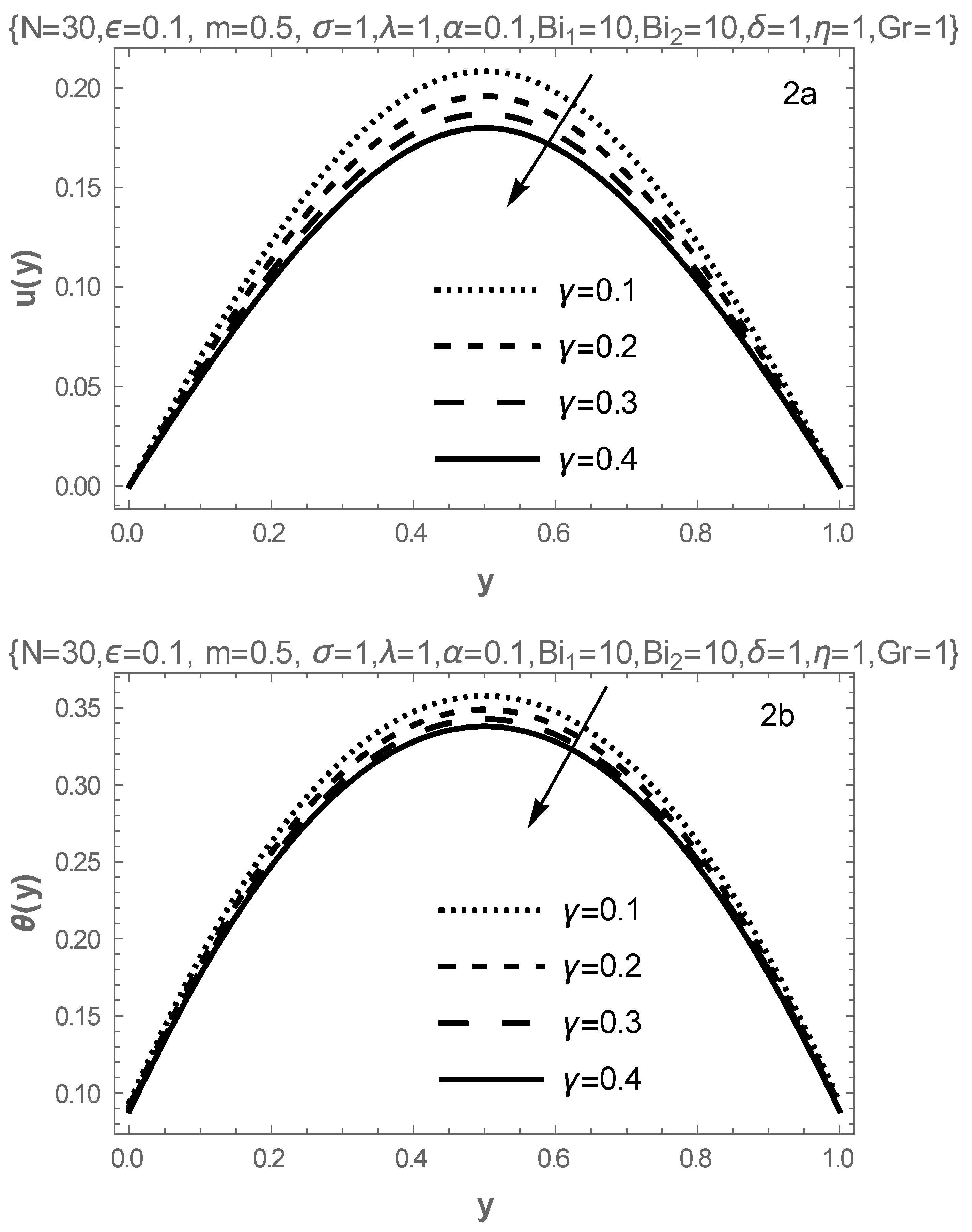
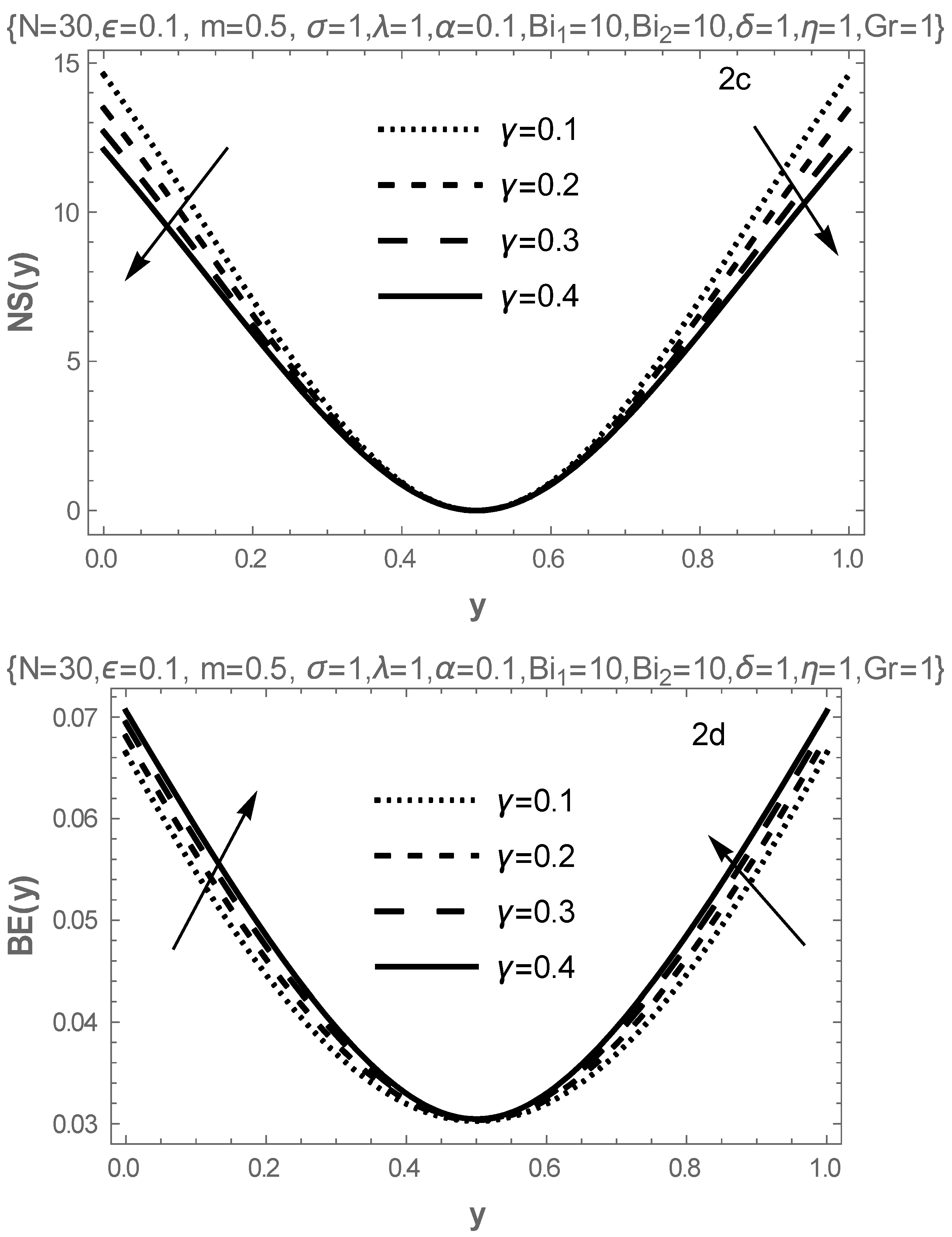
Increasing values of third-grade parameter encourages the thermal stability of the flow, while increasing values of the linear and nonlinear buoyancy parameter destabilizes the flow.
-
The Grashof number increase encourages the early occurrence of thermal runaway and exergy loss in the flow domain.
Future directions on this study are not limited to the developing flow, mass transfer, and elasto-hydrodynamics aspects of the work.

Author Contributions

Conceptualization, S.O.A.; Data curation, T.A.Y.; Formal analysis, S.O.A. and R.S.L.; Funding acquisition, R.S.L.; Investigation, T.A.Y.; Methodology, S.O.A.; Project administration, R.S.L.; Resources, T.A.Y.; Software, S.O.A.; Writing—original draft, S.O.A. All authors have read and agreed to the published version of the manuscript.

Funding

This research received no external funding.

Conflicts of Interest

The authors declare no conflict of interest.

Nomenclature

( x , y ) dimensional Cartesian coordinates, (m)
y dimensional Cartesian coordinates
T 0 referenced temperature, (K)
Tdimensional fluid temperature (K)
θ dimensionless fluid temperature
u the dimensional flow velocity (m/s)
u the dimensionless flow velocity
E activation energy (E/mols)
Q reaction heat (J)
C 0 initial specie concentration (mol)
A reaction rate constant
m reaction exponent
ε dimensionless activation energy
R universal rate constant J/(K.mol)
μ 0 constant dynamic viscosity (Poise)
ρ fluid density (Kg/m3)
g gravitational acceleration m/s2
Planck’s constant (Js)
υ frequency of vibration N.s/m2
P fluid pressure (N/m2)
k 0 referenced thermal conductivity J/(mK),
( α ¯ , η ¯ ) viscosity and thermal conductivity, respectively(1/K).
( α , η ) dimensionless variation parameters for viscosity and thermal conductivity, respectively.
G r modified Grashof number
σ coefficient of the quadratic thermal expansion,
λ Frank-Kameneskii parameter
δ Viscous dissipation parameter
B i Biot number
γ non-Newtonian material parameter
h 1 , 2 coefficient of heat transfer 1/K

References

  1. Salawu, S.O.; Fatunmbi, E.O.; Ayanshola, A.M. On the diffusion reaction of fourth-grade hydromagnetic fluid flow and thermal criticality in a plane couette medium. Results Eng. 2020, 8, 100169. [Google Scholar] [CrossRef]
  2. Cui, J.; Munir, S.; Raies, S.F.; Farooq, U.; Razzaq, R. Non-similar aspects of heat generation in bioconvection from flat surface subjected to chemically reactive stagnation point flow of Oldroyd-B fluid. Alex. Eng. J. 2022, 61, 5397–5411. [Google Scholar] [CrossRef]
  3. Salawu, S.O.; Oderinu, R.A.; Ohaegbue, A.D. Thermal runaway and thermodynamic second law of a reactive couple stress hydromagnetic fluid with variable properties and Navier slips. Sci. Afr. 2020, 7, e00261. [Google Scholar] [CrossRef]
  4. Sadiq, M.A.; Hayat, T. Entropy optimized flow of Reiner-Rivlin nanofluid with chemical reaction subject to stretchable rotating disk. Alex. Eng. J. 2022, 61, 3501–3510. [Google Scholar] [CrossRef]
  5. Okoya, S.S. Computational study of thermal influence in axial annular flow of a reactive third grade fluid with non-linear viscosity. Alex. Eng. J. 2019, 58, 401–411. [Google Scholar] [CrossRef]
  6. Adesanya, S.O.; Falade, J.; Jangili, S.; Bég, O.A. Irreversibility analysis for reactive third-grade fluid flow and heat transfer with convective wall cooling. Alex. Eng. J. 2017, 56, 153–160. [Google Scholar] [CrossRef] [Green Version]
  7. Salawu, S.O.; Kareem, R.A.; Shonola, S.A. Radiative thermal criticality and entropy generation of hydromagnetic reactive Powell–Eyring fluid in saturated porous media with variable conductivity. Energy Rep. 2019, 5, 480–488. [Google Scholar] [CrossRef]
  8. Makinde, O.D. Hermite-Padé approximation approach to thermal criticality for a reactive third-grade liquid in a channel with isothermal walls. Int. Commun. Heat Mass Transf. 2007, 34, 870–877. [Google Scholar] [CrossRef]
  9. Okoya, S.S. Disappearance of criticality for reactive third-grade fluid with Reynold’s model viscosity in a flat channel. Int. J. Non-Linear Mech. 2011, 46, 1110–1115. [Google Scholar] [CrossRef]
  10. Khan, S.A.; Khan, M.I.; Alzahrani, F. Melting heat transportation in chemical reactive flow of third grade nanofluid with irreversibility analysis. Int. Commun. Heat Mass Transf. 2021, 129, 105696. [Google Scholar] [CrossRef]
  11. Makinde, O.D.; Chinyoka, T. Numerical study of unsteady hydromagnetic generalized Couette flow of a reactive third-grade fluid with asymmetric convective cooling. Comput. Math. Appl. 2011, 61, 1167–1179. [Google Scholar] [CrossRef] [Green Version]
  12. Baranovskii, E.S.; Artemov, M.A. Steady flows of second-grade fluids in a channel. Appl. Math. 2017, 13, 342–353. [Google Scholar] [CrossRef]
  13. Okoya, S.S. On the transition for a generalized Couette flow of a reactive third-grade fluid with viscous dissipation. Int. Commun. Heat Mass Transf. 2008, 35, 188–196. [Google Scholar] [CrossRef]
  14. Hron, J.; LeRoux, C.; Malek, J.; Rajagopal, K.R. Flows of incompressible fluids subject to Navier’s slip on the boundary. Comput. Math. Appl. 2008, 56, 2128–2143. [Google Scholar] [CrossRef] [Green Version]
  15. Zehra, I.; Kousar, N.; UrRehman, K. Pressure dependent viscosity subject to Poiseuille and Couette flows via Tangent hyperbolic model. Phys. A Stat. Mech. Its Appl. 2019, 527, 121332. [Google Scholar] [CrossRef]
  16. Manjunatha, G.; Rajashekhar, C.; Vaidya, H.; Prasad, K.V.; Vajravelu, K. Impact of heat and mass transfer on the peristaltic mechanism of Jeffery fluid in a non-uniform porous channel with variable viscosity and thermal conductivity. J. Therm. Anal. Calorim. 2020, 139, 1213–1228. [Google Scholar] [CrossRef]
  17. Qasim, M.; Riaz, N.; Lu, D.; Afridi, M.I. Flow over a Needle Moving in a Stream of Dissipative Fluid Having Variable Viscosity and Thermal Conductivity. Arab. J. Sci. Eng. 2021, 46, 7295–7302. [Google Scholar] [CrossRef]
  18. Saraswathy, M.; Prakash, D.; Muthtamilselvan, M.; Al Mdallal, Q.M. Arrhenius energy on asymmetric flow and heat transfer of micropolar fluids with variable properties: A sensitivity approach. Alex. Eng. J. 2022, 61, 12329–12352. [Google Scholar] [CrossRef]
  19. Khan, A.A.; Zaib, F.; Zaman, A. Effects of entropy generation on Powell Eyring fluid in a porous channel. J. Braz. Soc. Mech. Sci. Eng. 2017, 39, 5027–5036. [Google Scholar] [CrossRef]
  20. Singh, K.; Pandey, A.K.; Kumar, M. Entropy generation impact on flow of micropolar fluid via an inclined channel with non-uniform heat source and variable fluid properties. Int. J. Appl. Comput. Math. 2020, 6, 85. [Google Scholar] [CrossRef]
  21. Shah, Z.; Kumam, P.; Deebani, W. Radiative MHD Casson Nanofluid Flow with Activation energy and chemical reaction over past nonlinearly stretching surface through Entropy generation. Sci. Rep. 2020, 10, 4402. [Google Scholar] [CrossRef] [PubMed] [Green Version]
  22. Yusuf, T.A.; Kumar, R.N.; Prasannakumara, B.C.; Adesanya, S.O. Irreversibility analysis in micropolar fluid film along an incline porous substrate with slip effects. Int. Commun. Heat Mass Transf. 2021, 126, 105357. [Google Scholar] [CrossRef]
  23. Agrawal, R.; Kaswan, P. Minimization of the entropy generation in MHD flow and heat transfer of nanofluid over a vertical cylinder under the influence of thermal radiation and slip condition. Heat Transf. 2022, 51, 1790–1808. [Google Scholar] [CrossRef]
  24. Adesanya, S.O.; Ogunseye, H.A.; Lebelo, R.S.; Moloi, K.C.; Adeyemi, O.G. Second law analysis for nonlinear convective flow of a reactive couple stress fluid through a vertical channel. Heliyon 2018, 4, e00907. [Google Scholar] [CrossRef] [Green Version]
  25. Xia, W.F.; Ahmad, S.; Khan, M.N.; Ahmad, H.; Rehman, A.; Baili, J.; Gia, T.N. Heat and mass transfer analysis of nonlinear mixed convective hybrid nanofluid flow with multiple slip boundary conditions. Case Stud. Therm. Eng. 2022, 32, 101893. [Google Scholar] [CrossRef]
  26. Ibrahim, W.; Gadisa, G. Finite element solution of nonlinear convective flow of Oldroyd-B fluid with Cattaneo-Christov heat flux model over nonlinear stretching sheet with heat generation or absorption. Propuls. Power Res. 2020, 9, 304–315. [Google Scholar] [CrossRef]
  27. Patil, P.M.; Shankar, H.F.; Hiremath, P.S.; Momoniat, E. Nonlinear mixed convective nanofluid flow about a rough sphere with the diffusion of liquid hydrogen. Alex. Eng. J. 2021, 60, 1043–1053. [Google Scholar] [CrossRef]
  28. Bandara, S.; Carnegie, C.; Johnson, C.; Akindoju, F.; Williams, E.; Swaby, J.M.; Oki, A.; Carson, L.E. Interaction of heat generation in nonlinear mixed/forced convective flow of Williamson fluid flow subject to generalized Fourier’s and Fick’s concept. J. Mater. Res. Technol. 2020, 9, 11080–11086. [Google Scholar]
  29. Yusuf, T.A.; Mabood, F.; Gbadeyan, J.A.; Adesanya, S.O. Nonlinear Convective for MHDOldroyd8-constant fluid in a channel with chemical reaction and convective boundary condition. J. Therm. Sci. Eng. Appl. 2020, 12, 1–19. [Google Scholar] [CrossRef]
  30. IjazKhan, M.; Alzahrani, F.; Hobiny, A. Heat transport and nonlinear mixed convective nanomaterial slip flow of Walter-B fluid containing gyrotactic microorganisms. Alex. Eng. J. 2020, 59, 1761–1769. [Google Scholar] [CrossRef]
  31. Ijaz, M.; Ayub, M. Nonlinear convective stratified flow of Maxwell nanofluid with activation energy. Heliyon 2019, 5, e01121. [Google Scholar] [CrossRef] [PubMed]
  32. Srinivasacharya, D.; RamReddy, C.; Naveen, P. Double dispersion effect on nonlinear convective flow over an inclined plate in a micropolar fluid saturated non-Darcy porous medium. Eng. Sci. Technol. Int. J. 2018, 21, 984–995. [Google Scholar] [CrossRef]
  33. Makinde, O.D. On thermal stability of a reactive third-grade fluid in a channel with convective cooling the walls. Appl. Math. Comput. 2009, 213, 170–176. [Google Scholar] [CrossRef]
  34. Makinde, O.D.; Aziz, A. Second law analysis for a variable viscosity plane Poiseuille flow with asymmetric convective cooling. Comput. Math. Appl. 2010, 60, 3012–3019. [Google Scholar] [CrossRef]
Figure 1. Flow geometry.
Mathematics 10 04276 g001
Figure 2. Variation of third-grade parameter.
Mathematics 10 04276 g002aMathematics 10 04276 g002b
Figure 3. Variations in Grashof number.
Mathematics 10 04276 g003aMathematics 10 04276 g003b
Figure 4. Variations in nonlinear Grashof number.
Mathematics 10 04276 g004aMathematics 10 04276 g004b
Figure 5. Variations in Frank-Kameneskii parameter.
Mathematics 10 04276 g005aMathematics 10 04276 g005b
Figure 6. Bifurcation plots when G r = 7 , σ = 0.1 = ε = η = α , δ = 0.2 , γ = 0.3 , B i 1 , 2 = 10 .
Mathematics 10 04276 g006
Table 1. Validation of numerical results for velocity δ = 0.5 , η = 0.1 , α = 0.3 , α = 0.1 , N = 30 ,   γ = 0.3 , G r = 1 ,   B i 1 = B i 2 = 10 ,   λ = 0.4 , ε = 0.1 , m = 0.5 .
y u ( y ) SCCM u ( y ) RK 4 | u ( y ) CWRM u ( y ) RK 4 |
0−6.96195549259×10−180.0000000000000006.961955492590054 × 10−18
0.10.043139418853409040.043139419937746051.084337016010739 × 10−9
0.20.078136340772973390.078136351909937721.11369643229775 × 10−8
0.30.104069771608132290.104069789210352061.760221977897824 × 10−9
0.40.120069903603826830.120069925676735592.207290876465872 × 10−8
0.50.125485273663029170.125485288887985961.522495679529001 × 10−9
0.60.120069903603826830.120069905332419871.728593046479432 × 10−9
0.70.10406977160813230.104069770221336931.386795372981808 × 10−9
0.80.078136340772973380.078136342285096851.512123468105919 × 10−9
0.90.0431394188534090440.043139419550354036.96944987832459 × 10−10
1.0−7.69196285588 × 10⁻¹⁸−9.12736796 × 10−109.12736788740352 × 10⁻¹⁰
Table 2. Validation of numerical results for temperature.
y θ ( y ) SCCM θ ( y ) RK 4 | θ ( y ) SCCM θ ( y ) RK 4 |
00.0221518490244846030.0221518493740973723.496127692903528 × 10−10
0.10.042084894473682670.042084890422843734.050838935121259 × 10−9
0.20.057515444347747080.0575154400066788954.341068185476082 × 10−9
0.30.068492684404716150.068492680311953164.092762989627019 × 10−9
0.40.075059305882255660.075059301979571133.902684536649659 × 10−9
0.50.077244674960420030.077244671423220923.537199116943057 × 10−9
0.60.075059305882255660.075059302826484293.055771372051374 × 10−9
0.70.068492684404716150.068492681677360712.727355438714163 × 10−9
0.80.057515444347747070.057515441806434392.541312688064678 × 10−9
0.90.042084894473682670.042084892202446412.271236268502896 × 10−9
1.00.0221518490244846030.022151847021219242.003265362621187 × 10−9
Table 3. Fast convergence of critical values by weighted residual method when G r = 3 , δ = 0.2 , B i 1 = 10 = B i 2 , m = 0.5 , ε = 0.1 .
N α σ γ η λ c
50.10.10.30.13.369629994329486
100.10.10.30.13.329979429762467
150.10.10.30.13.3377915382719980
200.10.10.30.13.3375451276368135
250.10.10.30.13.3376391452777585
300.10.10.30.13.3376334297519272
350.10.10.30.13.3376356319779727
Table 4. Thermal stability with values when δ = 0.2 , B i 1 = 10 = B i 2 , m = 0.5 , ε = 0.1 .
σ α γ η G r λ c
0.10.10.30.133.337791538271998
0.30.10.30.133.294547099649542
0.50.10.30.133.251342585235665
0.10.30.30.133.327113416799457
0.10.50.30.133.3180031889548034
0.10.10.50.133.354693697420452
0.10.10.80.133.370237078964153
0.10.10.30.0133.5150936154732557
0.10.10.30.00133.5341579072708558
0.10.10.30.153.1911369048073452
0.10.10.30.173.0387490555917243
Table 5. Validation with previous result when B i 1 = B i 2 = 10 , G r = 0 = γ = η , α = 0.1 .
y u 1 ( y )
Makinde & Aziz [34]
u 2 ( y )
Present Result
| u 1 ( y ) u 2 ( y ) |
00.00000000000000001.9996146847 × 10−181.999614684734152 × 10⁻¹⁸
0.10.045002608972707280.045002617690366078.717658789292315 × 10−9
0.20.080005421992315030.080005431513844629.521529592548816 × 10−9
0.30.105007673227255570.105007683076116969.848861393102482 × 10−9
0.40.120009070004462120.120009080684472111.068000998749596 × 10−8
0.50.125009542657467250.125009549331961546.674494290592747 × 10−9
0.60.120009076503442110.120009080684472114.181029994443364 × 10−9
0.70.105007680804126770.105007683076116982.271990207081131 × 10−9
0.80.080005431087961860.080005431513844614.258827457359615 × 10−10
0.90.0450026178034514950.045002617690366071.130854229702826 × 10−10
1.08.38288175864 × 10−102.13968421631 × 10−188.38288173724192 × 10⁻¹⁰
Table 6. Validation with previous result when B i 1 = B i 2 = 10 , G r = 0 = γ = η , α = 0.1 .
y θ 1 ( y ) S R K 4
Makinde & Aziz [34]
θ 2 ( y ) S C C M
Present Result
| θ 1 ( y ) θ 2 ( y ) |
00.00041669597326112980.000416696430798102364.57536972555978 × 10−10
0.10.00072420785688684990.00072422042309931131.256621246132922 × 10−8
0.20.00087005896090012640.00087006655168444157.59078431502528 × 10−9
0.30.00092423124987068790.00092423820303720556.953166517597101 × 10−9
0.40.00093673306067154110.00093673937120818556.310536644453524 × 10−9
0.50.00093756713713157450.00093757278265770185.645526127313893 × 10−9
0.60.0009367343399450980.00093673937120818555.031263087466702 × 10−9
0.70.00092423378807235140.00092423820303720524.414964853774461 × 10−9
0.80.00087006276113259150.00087006655168444113.790551849616394 × 10−9
0.90.00072421727472966610.00072422042309931073.148369644634038 × 10−9
1.00.00041669394316600920.00041669643079810192.487632092722583 × 10−9
Publisher’s Note: MDPI stays neutral with regard to jurisdictional claims in published maps and institutional affiliations.

