Statistical Inference for Competing Risks Model with Adaptive Progressively Type-II Censored Gompertz Life Data Using Industrial and Medical Applications

Abstract

This study uses the adaptive Type-II progressively censored competing risks model to estimate the unknown parameters and the survival function of the Gompertz distribution. Where the lifetime for each failure is considered independent, and each follows a unique Gompertz distribution with different shape parameters. First, the Newton-Raphson method is used to derive the maximum likelihood estimators (MLEs), and the existence and uniqueness of the estimators are also demonstrated. We used the stochastic expectation maximization (SEM) method to construct MLEs for unknown parameters, which simplified and facilitated computation. Based on the asymptotic normality of the MLEs and SEM methods, we create the corresponding confidence intervals for unknown parameters, and the delta approach is utilized to obtain the interval estimation of the reliability function. Additionally, using two bootstrap techniques, the approximative interval estimators for all unknowns are created. Furthermore, we computed the Bayes estimates of unknown parameters as well as the survival function using the Markov chain Monte Carlo (MCMC) method in the presence of square error and LINEX loss functions. Finally, we look into two real data sets and create a simulation study to evaluate the efficacy of the established approaches.

1. Introduction

In practical applications, especially in medical fields and engineering sciences, lifetime studies are a useful tool to investigate the survival unit distribution. When analyzing data from these studies, an important component is the assumed lifetime distribution. Some common lifetime distributions include the exponential, generalized exponential, Rayleigh, Pareto, and Weibull, to name a few. Besides these common life distributions, the Gompertz distribution (Gompertz [1]) is also frequently used to analyze lifetime data. Further, it is used to describe growth in plants, animals, bacteria, and cancer cells, see Willemse and Koppelaar [2]. In recent studies, the Gompertz model has been successfully used to characterize growth curves in many fields, including biology, crop science, medicine, engineering, computer science, economics, marketing, human mortality, human demographics, and actuarial mortality, to name a few. Due to the recent global spread of COVID-19 cases, this distribution has been used to predict and estimate the number of COVID-19 cases in different countries. For instance, Rodriguez et al. [3] predicted a different number of COVID-19 cases in Mexico using the Gompertz model. According to Jia et al. [4], the Gompertz model has been applied successfully to forecast the amount of COVID-19 infections in China. The Gompertz distribution is thus worthwhile to investigate in this paper due to its numerous uses and applications.

The mathematical symbols for the probability density function (PDF) and cumulative distribution function (CDF) related to the Gompertz distribution are given, respectively, by

$$f(x;\theta ,\lambda )=\theta e^{\lambda x}exp\left\{-\frac{\theta }{\lambda }\left(e^{\lambda x}-1\right)\right\},x>0,\lambda ,\theta >0,$$

(1)

and

$$F(x;\theta ,\lambda )=1-exp\left\{-\frac{\theta }{\lambda }\left(e^{\lambda x}-1\right)\right\},x\ge 0,\lambda ,\theta >0.$$

(2)

The reliability or survival function and the failure rate function become, respectively

$$S\left(t\right)=exp\left\{-\frac{\theta }{\lambda }\left(e^{\lambda t}-1\right)\right\}\mathrm{and}h\left(t\right)=\theta e^{\lambda t},t\ge 0,\lambda ,\theta >0,$$

(3)

where, $\lambda >0$ is the scale parameter and $\theta >0$ is the shape parameter. The failure rate (hazard) function $h\left(t\right)$ increases or decreases monotonically, and the log($h\left(t\right)$) is linear with t. It is known Gompertz distribution is a flexible model that can be skewed to the left or the right by varying the values of $\theta$ and $\lambda$. Where the parameter $\lambda$ satisfies the criteria listed below:

• If $0<\lambda \le \theta$, then $\frac{df(x;\theta ,\lambda )}{dx}<0,$ where $x>0$, hence $f(x;\theta ,\lambda )$ is monotonically decreasing.
• If $\lambda >\theta$, the PDF (1) will monotonically increase when $x\in (0,\frac{ln\lambda /\theta }{\lambda })$ and decrease when $x\in (\frac{ln\lambda /\theta }{\lambda },\infty ).$
• If $\lambda <1$, then the hazard monotonically decreases over time t.
• If $\lambda >1$, the hazard then monotonically increases with time $t.$
• When $\lambda \to 0$, the Gompertz distribution tends to become exponential.

The inference of the unknown lifetime parameters of the Gompertz distribution based on censoring data has been widely discussed in the last two decades. Including, for example, Jaheen [5] investigated this distribution based on progressive Type-II censoring using a Bayesian methodology. Also, based on progressive Type-II censored samples, Wu et al. [6] developed point and interval estimators for the parameters of the Gompertz distribution. Wu et al. [7] explored the estimation of Gompertz distribution with a Type-II progressive censoring scheme, where the units are randomly removed. Ismail [8] used step stress partially accelerated life tests with two stress levels and Type-I censoring and the Gompertz distribution as a life model to apply the Bayesian technique to the estimation problem. The point and interval estimations of a two-parameter Gompertz distribution under partially accelerated life tests with Type-II censoring were also covered by Ismail [9]. Soliman et al. [10] have dealt with parameter estimation using progressive first-failure censored data. Soliman and Al Sobhi [11] analyzed first-failure progressive data to deal with the estimation of Gompertz distribution. The Bayes estimation and expected termination time for the competing risks model for the Gompertz distribution under progressively hybrid censoring with binomial removals have been taken into consideration by Wu and Shi [12]. The statistical inference for the Gompertz distribution with Type-II progressive hybrid data and generalized progressively hybrid censored data have been covered in El-Din et al. [13].

Due to resource shortages, time restraints, employee changes, and accidents, data cannot be fully completed in practice when studying lifetime experiments. Experimenters use filtering or censoring techniques to shorten testing times and associated expenses. The two most common forms of censored systems in literature are Type-I and Type-II. With Type-I censoring, the test is over at a pre-fixed time, whereas with Type-II censoring, only the first m failed units in a random sample of size n ($m<n$) are observed. Or equivalent, the experiment stops when it collects a specified amount of data. Although this method is easy to implement, it has the potential to waste a lot of test time. Furthermore, until the test is over, no unit can be taken out of it. In order to increase the effectiveness of the experiment, progressive Type-II censoring was suggested. With this censoring method, test units can be eliminated at different points throughout the experiment. We refer to Balakrishnan and Cramer [14] for additional information. The following illustrates how the progressive Type-II censoring model works.

Denote $X_1$, $X_2,\dots ,$ $X_n$ as the respective lifetimes of the n units that are placed on a life test. the progressive Type-II censoring scheme $\Re =$($R_1,R_2,\dots ,R_m$) and the number of units observed m ($m<n$) are determined before the experiment. $R_i>0,$ $i=1,2,\dots ,m$ and $n=m+{\displaystyle \sum _{i=1}^m}{R}_i$. The remaining $R_i$ units are arbitrarily removed from the experiment once the ith failure is noticed. As long as this rule is followed, the experiment will continue until m failures are observed and here the experiment ends. As a result, the observed statistics for the progressive Type-II right censoring order are ($X_{1:m:n}$, $X_{2:m:n}$,….,$X_{m:m:n}$). This model simulates the real-world scenario where some units are lost or removed throughout the experiment, which makes it more logical than Type-II censoring. Even while progressive censorship can considerably increase the effectiveness of the experiment, the trial’s runtime is frequently still too long. In many cases, it is important to know how long before a particular event occurs, especially in clinical research. Ng et al. [15] suggested adaptive Type-II progressive censoring to improve the effectiveness of statistical inference and reduce overall test duration. This plan operates as follows: Consider putting n identical units through a life test. The observed number of failures $m(m<n)$ is predetermined, and the test time is permitted to extend beyond the time T that is specified beforehand. The progressive censoring method ℜ is specified, although some of the $R_i\prime s$ values may change accordingly during the life test. As explained above, after the ith failure is noticed during the life test, $R_i$ units are at random removed from the test. We write $X_{i:m:n}$, $i=1,2,\dots ,m$, to represent the m fully observed lifetimes. If the mth failure time occurs before time T (i.e. $X_{m:m:n}<T$), the test ends at time $X_{m:m:n}$ using the same progressive censoring scheme ($R_1,R_2,\dots ,R_m$), where $R_m=n-m-{\displaystyle \sum _{i=1}^{m-1}}{R}_i$. If Jth failure time happens before time T, i.e., $X_{J:m:n}<T<X_{J+1:m:n},(1\le J\le m-1)$, where $X_{0:m:n}\equiv 0$ and $X_{m+1:m:n}\equiv \infty$, then we adapt the number of units progressively withdrawn from test upon failures by setting $R_{J+1}=R_{J+2}=\dots =R_{m-1}=0$, and at the time $X_{m:m:n}$ all remaining units $R_m$ are eliminated, where $R_m=n-m-{\displaystyle \sum _{i=1}^J}{R}_i$. So, in this situation, the effectively applied progressive censored scheme is ($R_1,R_2,\dots ,R_J,0,0,\dots ,0,n-m-{\displaystyle \sum _{i=1}^J}{R}_i$). In this study, we employ $X_i$ instead of $X_{i:m:n}$; $i=1,2,\dots ,m$. One of the following two scenarios might represent the observed data under-considered censoring scheme:

Case 1$:(X_1,R_1),(X_2,R_2),\dots ,(X_m,R_m)$, if $X_m<T$, where $R_m=n-m-{\displaystyle \sum _{i=1}^{m-1}}{R}_i,$

Case 2$:(X_1,R_1),\dots ,(X_J,R_J),(X_{J+1},0),\dots ,(X_{m-1},0),(X_m,R_m)$, if $X_J<T<X_{J+1}$.

It should be noted that Type-II and Type-II progressive censoring schemes are both extensions of the the adaptive Type-II censored scheme. While adaptive Type-II censored scheme reduces to Type-II censoring scheme if $T=0$, $J=0$, no units will be removed, and if $T=1$, $J=m$, $R_i$($i=1,2,\dots ,m$) survival units will be eliminated at random during the trial, adaptive Type-II censored scheme is exactly Type-II progressive censored scheme.

There have been a lot of discussions recently about the adaptive Type-II censored scheme. As an illustration, Sobhi and Soliman [16] worked with the exponentiated Weibull distribution, they investigated the estimate of its parameters, reliability, and hazard functions. They employed the approach of Bayesian estimation as well as the MLE under the adaptive Type-II censored scheme. ML and Bayes estimates for the unknown parameters of the inverse Weibull distribution under the adaptive Type-II censored scheme were described by Nassar and Abo-Kasem [17]. According to the adaptive Type-II censored scheme, Sewailem and Baklizi [18] investigated the ML and Bayes estimates for the log-logistic distribution parameters. The estimations of entropy for inverse Weibull distributions using the adaptive Type-II censored scheme were developed by Xu and Gui [19]. The parameters of an exponentiated inverted Rayleigh model were calculated by Panahi and Moradi [20]. They studied the MLE and Bayesian analysis under an adaptive Type-II censored hybrid censored scheme. Chen and Gui [21] concentrated on a statistical analysis of the Chen and Gui Chen model with adaptive progressive Type-II censoring. Kumarswamy-exponential distribution was taken into consideration in the adaptive progressive Type-II censoring technique by Mohan and Chacko [22]. Under the adaptive progressive Type-II censoring scheme, Hora et al. [23] considered the classical and Bayesian inferences for unknown parameters of the inverse Lomax distribution. Recently, using the adaptive Type-II progressive censored sample from the Gompertz distribution, Amein et al. [24] examined several estimation strategies.

The adaptive Type-II progressive censored is used in this paper instead of Type-I, Type-II, and Type-II progressive censored schemes because it favors experiments where units must be disassembled at different stages of failure before the appropriate intended sample size is reached and also has a predetermined time during which the experiment can occur.

In some medical or engineering studies, individuals may fail due to different failure causes. In literature, it refers to the competing risks model. According to the competing risks model, observable data include the individual failure time and a cause-of-failure indicator. These failure factors might or might not be independent. In most cases, when analyzing data on competing risks, the failure factors are considered to be independent of each other. For example, a patient can die from breast cancer or stroke, but he cannot die from both. In the same field, when studying thyroid cancer, three causal factors play a possible role in thyroid cancer. The first is radiation exposure, the second is an elevated level of thyroid-stimulating hormone, and the third suggested factor is prolonged exposure to iodine deficiency. Based on the assessment of these factors, patients are divided into low or high-risk groups.

Another example is applied in the industrial and mechanical fields, an assembly device may fail to break the welding/bond plate front due to fatigue, or low electrical/optical signal (voltage, current, or light intensity) to an unacceptable level due to aging deterioration. In this example, the electronic product fails due to two independent elements of failure: welding interface fracture (catastrophic failure or difficult failure) and brightness of electrical/optical signal reductions (degradation failure or fine failure). Crowder [25] is a reliable source for a comprehensive investigation of several competing risk models.

Many academics have recently studied statistical inference for the parameters of various lifetime parametric models utilizing various censoring techniques with competing risk data. Kundu et al. [26], for instance, took into account the analysis of competing risks data when the data are progressively Type-II censored from exponential distributions. Based on progressive Type-II censoring of competing risks, Pareek et al. [27] determined the MLEs of the parameters of Weibull distributions and their asymptotic variance-covariance. When the lifetime distributions are Weibull distributions, Kundu and Pradhan [28] studied the Bayesian inference of the unknown parameters of the progressively censored competing risks data. The estimators of the parameters for Lomax distributions were determined by Cramer and Schmiedt [29] using a progressive Type-II censoring competitive risks model. For the distribution parameters, they calculated the expected Fisher information matrices and MLEs. Generalized exponential distribution with adaptive Type-II progressive hybrid censored competing risks data was studied by Ashour and Nassar [30]. A competing risks model with a generalized Type I hybrid censoring method was presented by Mao et al. [31]. They estimated both exact and approximate confidence intervals using the exact distributions, asymptotic distributions, and parametric bootstrap approaches, respectively. Wu and Shi [12] developed the Bayes estimation for the two-parameter Gompertz distribution competitive risks model under Type-I gradually hybrid censoring scheme with binomial removals. The point estimate and point prediction for a class of an exponential distribution with Type-I progressively interval-censored competing risks data were studied by Ahmadi et al. [32]. Dey et al. [33] took into account the Bayesian analysis of modified Weibull distribution under progressively censored competing risk models. Inference techniques for the Weibull distribution under adaptive Type-I progressive hybrid censored competing risks data are described by Ashour and Nassar [34]. Additionally, a competing risk model using exponential distributions and the adaptive Type-II progressively censoring scheme is also taken into account by Hemmati and Khorram [35]. They developed MLEs of unknown parameters and constructed the confidence intervals as well as the two different bootstraps of different unknown parameters. The Bayes estimates and associated two-sides probability intervals were also likewise driven by them. Azizi et al. [36] considered statistical inference for a competing risks model using Weibull data with progressive interval censoring. Based on progressive Type-II censored competing risks data with binomial removals, Chacko and Mohan [37] developed the Bayesian analysis of the Weibull distribution. Baghestani and Baharanchi [38] investigate an improper Weibull distribution for competing for risk analysis using a Bayesian technique. The statistical inference of the Burr-XII distribution under progressive Type-II censored competing risks data with binomial removals has been studied by Qin and Gui [39]. Progressive Type-II censored competing risks data from the linear exponential distribution have been examined by Davies and Volterman [40]. In the adaptive Progressive Type-II censored model with independent competing risks, Ren and Gui [41] proposed several of statistical inference techniques to estimate the parameters and reliability of the Weibull distribution. Recent research by Lodhi et al. [42] examined a competing risks model utilizing the Gompertz distribution under progressive Type-II censoring where failure cause probability distributions are identically distributed with a similar scale and variable shape parameters.

The major goal of this research is to analyze the adaptive progressively Type-II censored with competing risks sample from the Gompertz distribution because there aren’t many relevant works that deal with adaptive progressively Type-II censored competing risks data. The model parameters and reliability function are estimated using the maximum likelihood method. In this method, with the help of the graphical method, developed by Balakrishnan and Kateri [43], the issue of the starting value of the MLEs is resolved here. The existence and uniqueness of the MLEs of the model parameters are established. The Newton-Rapshon (NR) method and the stochastic expectation-maximization (SEM) algorithm are the two algorithms that are being taken into consideration to numerically determine the MLEs for the parameters. We cover interval estimation using the two approximation information matrix methods and the bootstrap method. With the assumption that the model parameters follow independent gamma priors for the two different shape parameters and inverted gamma for the scale parameter, the Bayes estimators and associated credible intervals are then obtained using the Metropolis-Hasting (MH) algorithm based on squared error (SE) and linear-exponential (LINEX) loss functions. Last but not least, through Monte Carlo simulation, the performances of estimates are assessed using average bias and mean squared error (MSE) for point estimation and average length and probability coverage for interval estimation.

The remaining portions of this article are structured as follows: We describe the model in Section 2 of the paper. The MLEs of the unknown parameters based on the NR and SEM techniques are discussed in Section 3 of this article. We also present the estimated confidence intervals using the corresponding MLEs’ normalcy requirement. In Section 4, The bootstrap confidence intervals for the unknown parameters as well as the reliability function are obtained. The Markov chain Monte Carlo (MCMC) approach is used in Section 5 to approximate the Bayesian estimates and to generate MCMC intervals for the unknowns. Section 6 presents a Monte Carlo simulation analysis that contrasts the results of the various approaches. This part also introduces actual data sets to demonstrate the efficacy of the methods used in this paper. Several conclusions are provided as a conclusion in Section 7.

2. Model Assumptions

In this light, failure times have an independent Gompertz distribution and two different causes for failure. As a result, the cause-specific density function for the random variable $X_{ik}$, $k=1,2$ is given by

$$f_k(x;\vartheta )={\theta }_k{e}^{\lambda x}exp\left\{-\frac{{\theta }_k}{\lambda }\left(e^{\lambda x}-1\right)\right\},x>0,\lambda ,{\theta }_k>0,k=1,2,$$

(4)

and the cause specific survival (reliability) function is defined as

$${\overline{F}}_k(x;\vartheta )=exp\left\{-\frac{{\theta }_k}{\lambda }\left(e^{\lambda x}-1\right)\right\},x>0,\lambda ,{\theta }_k>0,k=1,2,$$

(5)

where item’s lifetime is shown as $X_i$, $i=1,2,\dots ,n$ and the time the element i fails as a result of cause k is $X_i$, where $X_i=min\{X_{i1},X_{i2}\}$.

Remark 1.

If$X_1\sim$Gompertz(${\theta }_1,\lambda$) and$X_2\sim$Gompertz(${\theta }_2,\lambda$) are mutually independent random variables, then the survivor function of $X=min\{X_1,X_2\}$is a Gompertz random variable with scale parameter$\left({\theta }_1+{\theta }_2\right)$and shape parameter λ. Suppose $\overline{F}\left(x\right)$is a surviving function of X that may be obtained by

$$\begin{array}{ccc}\hfill \overline{F}\left(x\right)& =& P\left(min\{X_1,X_2\}>x\right)=P\left(X_1>x\right)P\left(X_2>x\right)\hfill \\ & =& {\overline{F}}_{{}_1}\left(x\right){\overline{F}}_{{}_2}\left(x\right)=exp\left\{-\frac{{\theta }_1}{\lambda }\left(e^{\lambda x}-1\right)\right\}exp\left\{-\frac{{\theta }_2}{\lambda }\left(e^{\lambda x}-1\right)\right\}=exp\left[-\frac{\left({\theta }_1+{\theta }_2\right)}{\lambda }\left(e^{\lambda x}-1\right)\right].\hfill \end{array}$$

Consequently, the cumulative distribution function ($F\left(x\right)$) and probability density function ($f\left(x\right)$) are given by

$$F\left(x\right)=1-exp\left[-\frac{\left({\theta }_1+{\theta }_2\right)}{\lambda }\left(e^{\lambda x}-1\right)\right]\mathrm{and}f\left(x\right)=\left({\theta }_1+{\theta }_2\right)e^{\lambda x}exp\left[-\frac{\left({\theta }_1+{\theta }_2\right)}{\lambda }\left(e^{\lambda x}-1\right)\right].$$

(6)

The life test experiment is ended with an adaptive progressively Type-II censoring system under competing risks Gompertz models when the number of failures exceeds $m<n$. The following algorithm is then used to create the random sample of total lifetime X:

A1:

Generate two i.i.d samples of size n for each cause of failure as follows:

$$(X_{11},X_{21},\dots ,X_n)\stackrel{i.i.d}{\backsim }\mathrm{Gompertz}({\theta }_1,\lambda )\mathrm{and}(X_{12},X_{22},\dots ,X_n)\stackrel{i.i.d}{\backsim }\mathrm{Gompertz}({\theta }_2,\lambda ),$$

A2:

For each $i=1,\dots ,n,$ If $X_{i1}\le X_{i2}$ set ${\delta }_i=1$ and $X_i=X_{i1}$, else, if $X_{i1}>X_{i2}$ set ${\delta }_i=2$ and $X_i=X_{i1}$. We now have the data as follows.$(X_1,{\delta }_1),(X_2,{\delta }_2),\dots ,(X_n,{\delta }_n)$. Set $n_1=\{\#X_i:X_i\in X_{i1}\}$, $n_2=\{\#X_i:X_i\in X_{i2}\}$, and $n=n_1+n_2$.

A3:

This is now ordered irrespective of the cause of failure, but without losing track of the corresponding cause of failure. Thus we now have the n usual order statistics.$(X_{1:n},{\delta }_1)$, $(X_{2:n},{\delta }_2)$, …, $(X_{n:n},{\delta }_n)$.

A4:

In advance of the experiment, the number of units observed m ($m<n$) and the Type-II progressive censoring scheme $\Re =$($R_1,R_2,\dots ,R_m$) are both determined, where $R_i>0,i=1,2,m$ and ${\displaystyle \sum _{i=1}^m}{R}_i=n+m$.

A5:

To begin with $X_{1:n}$ is observed as the first failure and thus $X_{1:m:n}=X_{1:n}$. Then $R_1$ of the $n-1$ units that are still alive are chosen at random and removed from the experiment. At this point, the second failure is observed as the next smallest lifetime of the remaining units, i.e., ($X_{2:m:n}$), and as a result, $R_2$ of the remaining $n-R_1-2$ units are arbitrarily censored from the study. This procedure is carried out repeatedly until all of the remaining $R_m=n-m-{\displaystyle \sum _{i=1}^{m-1}}{R}_i$ units are censored at the time of the mth observed failure ($X_{m:m:n}$). We now have a progressively Type-II censoring data $(X_{1:m:n},{\delta }_1^{*}),(X_{2:m:n},{\delta }_2^{*}),\dots ,(X_{m:m:n},{\delta }_m^{*})$, where we introduce the notation ${}^{*}$ since ${\delta }_i^{*\prime }s$ are concomitants of the order statistics. Thus, ${\delta }_i^{*}$ may not be equal to ${\delta }_i.$

A6:

Here, the expression ${\delta }_i^{*}=k$, $k=1,2$ indicates that the failure of unit i at time $X_{i:m:n}$ was failed by cause k. Let $I_k\left(A\right)$ is the indicator of the event A, where

$$I_1({\delta }_i^{*}=1)=\left\{\begin{array}{c}1,{\delta }_i^{*}=1\\ 0\mathrm{else}\end{array}\right.\mathrm{and}{I}_2({\delta }_i^{*}=2)=\left\{\begin{array}{c}1,{\delta }_i^{*}=2\\ 0\mathrm{else}\end{array}\right..$$

The number of failures attributable to the first and second causes of failure, respectively, are thus described by the random variables $m_1=\sum _{i=1}^{m}I({\delta }_i^{*}=1)$ and $m_2=\sum _{i=1}^{m}I({\delta }_i^{*}=2)$, where $m_1+m_2=m$, and $m>0.$

A7:

Let’s say a test has a predetermined expected completion time T, but we allow the total test time to exceed T. When $X_{m:m:n}<T$, the life testing experiment comes to an end. In the absence of this, the experiment ends when $X_{J:m:n}<T<X_{J+1:m:n},(1\le J\le m-1)$. We don’t discard any survival unit, it means that the censoring scheme ℜ will be changed to $R_{J+1}=R_{J+2}=\dots =R_{m-1}=0,R_m=n-m-\sum _{j=1}^J{R}_j$. where $J=max\{j:X_{j:m:n}<T\}$. Thus, under the adaptive Type-II progressive censoring scheme and in presence of competing risks data, our observations are of the form $(X_{1:m:n},{\delta }_1^{*},R_1)$, …, $(X_{J:m:n},{\delta }_J^{*},R_J)$, $(X_{J+1::m:n},{\delta }_{J+1}^{*},0)$, …, $(X_{m-1:m:n},{\delta }_{m-1}^{*},0)$, $(X_{m:m:n},{\delta }_{m-1}^{*},R_m)$.

3. Maximum Likelihood Estimation

In this section, we look at the issue of constructing maximum likelihood estimators (MLEs), their confidence intervals for unknown parameters, and the reliability function of the Gompertz distribution using the adaptive Type-II progressive censoring scheme and competing risks data. Here, it is suggested to estimate the unknown parameters using the NR and SEM algorithms. These two algorithms each have benefits and drawbacks. In this case, the SEM algorithm outperforms the NR algorithm by avoiding saddle points and resolving the issues with local maxima by repeatedly simulating new values. Moreover, the calculations are accelerated and made simpler by the NR approach. Therefore, it can be challenging to select one algorithm over another. It might be preferable to consider the two strategies as alternatives and do a numerical search to assess how the outcomes respond to each technique.

3.1. MLE via Newton–Raphson Procedure

According to the previously mentioned assumptions, the likelihood function of the competing risk model can be expressed as follows (see Kundu et al. [26])

$$L\left(\vartheta ;\mathbf{x}\right)=C_J\prod _{i=1}^m{\left[f_1\left(x_i\right)\left({\overline{F}}_2\left(x_i\right)\right)\right]}^{I\left({\delta }_i=1\right)}\left\{{\left[f_2\left(x_i\right)\left({\overline{F}}_1\left(x_i\right)\right)\right]}^{I\left({\delta }_i=2\right)}\right\}\prod _{i=1}^J{\left[\overline{F}\left(x_i\right)\right]}^{R_i}{\left[\overline{F}\left(x_m\right)\right]}^{R^{*}},$$

(7)

where

$$C_J=\prod _{i=1}^m(n-i+1-\sum _{j=1}^{max\{i-1,J\}}{R}_j,),R^{*}=n-m-\sum _{i=1}^J{R}_i,\mathrm{and}{\overline{F}}_k\left(x_i\right)=1-F_k\left(x_i\right),k=1,2$$

From (1), (2) and (7), we obtain the likelihood function of observed sample data X, it can be written as

$$L\left(\vartheta ;\mathbf{x}\right)=C_J{\theta }_1^{m_1}{\theta }_2^{m_2}{e}^{\lambda {\sum }_{i=1}^m{x}_i}exp\left\{-\frac{A(\mathbf{x},\lambda ){\sum }_{k=1}^2{\theta }_k}{\lambda }\right\},$$

(8)

where

$$A(\mathbf{x},\lambda )=\sum _{i=1}^m\left(e^{\lambda x_i}-1\right)+\sum _{i=1}^J{R}_i\left(e^{\lambda x_i}-1\right)+R^{*}\left(e^{\lambda x_m}-1\right).$$

(9)

The additive constant $C_J$ is ignored by the log-likelihood function, which is given by:

$$\mathcal{L}\left(\vartheta ;\mathbf{x}\right)\sum _{k=1}^2{m}_{k}log{\theta }_k+\lambda \sum _{i=1}^m{x}_i-\frac{A(\mathbf{x},\lambda ){\sum }_{k=1}^2{\theta }_k}{\lambda },$$

The log-likelihood function’s first order derivatives with respect to ${\theta }_1$, ${\theta }_2$ and $\lambda$ are given by

$$\frac{\partial \mathcal{L}\left(\vartheta ;\mathbf{x}\right)}{\partial {\theta }_k}=\frac{m_k}{{\theta }_k}-\frac{A(\mathbf{x},\lambda )}{\lambda }=0,k=1,2,$$

(10)

and

$$\frac{\partial \mathcal{L}\left(\vartheta ;\mathbf{x}\right)}{\partial \lambda }=\sum _{i=1}^m{x}_i+\frac{{\sum }_{k=1}^2{\theta }_k}{\lambda }\left\{\frac{A(x,\lambda )}{\lambda }-B(\mathbf{x},\lambda )\right\}=0,$$

(11)

where, $A(x,\lambda )$ is given by (9) and $B(\mathbf{x},\lambda )={\sum }_{i=1}^m{x}_i{e}^{\lambda x_i}+{\sum }_{i=1}^J{R}_i{x}_i{e}^{\lambda x_i}+R_m{x}_m{e}^{\lambda x_m}.$

From Equation (10), the MLE of ${\theta }_k$ is given by

$${\widehat{\theta }}_k\left(\lambda \right)=\frac{m_k\widehat{\lambda }}{A(\mathbf{x},\widehat{\lambda })},k=1,2.$$

(12)

Theorem 1.

Assume that under an adaptive Type-II progressively censoring scheme, the failure rates for the competing risks follow the Gompertz distribution with different parameters ${\theta }_1$ and ${\theta }_2$, for ${\theta }_1>0$, ${\theta }_2>0$ and $\lambda >0$, the MLE of ${\theta }_k$, $k=1,2$ exists and is given by (12).

Proof. 

Since $logt\le t-1$, $t>0$ holds and let $t=\frac{{\theta }_k}{{\widehat{\theta }}_k},$ then

$$\begin{array}{ccc}\hfill m_{k}log{\theta }_k& =& m_{k}log\frac{{\theta }_k}{{\widehat{\theta }}_k}+m_{k}log{\widehat{\theta }}_k\hfill \\ & \le & m_k\frac{{\theta }_k}{{\widehat{\theta }}_k}-m_k+m_{k}log{\widehat{\theta }}_k\hfill \\ & =& \frac{{\theta }_{k}A(\mathbf{x},\lambda )}{\lambda }-m_k+m_{k}log{\widehat{\theta }}_k.\hfill \end{array}$$

Which implies that

$$\begin{array}{ccc}\hfill \mathcal{L}\left(\vartheta ;\mathbf{x}\right)\hspace{1em}\propto & & \sum _{k=1}^2{m}_{k}log{\theta }_k+\lambda \sum _{i=1}^m{x}_i-\frac{{\sum }_{k=1}^2{\theta }_k}{\lambda }A(\mathbf{x},\lambda )\hfill \\ & \le & \sum _{k=1}^2\left[\frac{{\theta }_{k}A(\mathbf{x},\lambda )}{\lambda }-m_k+m_{k}log{\widehat{\theta }}_k\right]+\lambda \sum _{i=1}^m{x}_i-\frac{{\sum }_{k=1}^2{\theta }_k}{\lambda }A(\mathbf{x},\lambda ).\hfill \end{array}$$

□

From (12), by using

$$m_k=\frac{{\widehat{\theta }}_{k}A(\mathbf{x},\lambda )}{\lambda },$$

then we have

$$\mathcal{L}\left(\vartheta ;\mathbf{x}\right)\le \sum _{k=1}^2{m}_{k}log{\widehat{\theta }}_k+\lambda \sum _{i=1}^m{x}_i-\frac{{\sum }_{k=1}^2{\theta }_k}{\lambda }A(\mathbf{x},\lambda )=\mathcal{L}\left(\widehat{\vartheta };\mathbf{x}\right)$$

Equality holds if and only if ${\theta }_1={\widehat{\theta }}_k$, $k=1,2.$

By omitting the constant and substituting ${\widehat{\theta }}_k\left(\lambda \right)$ into $\mathcal{L}\left(\vartheta ;\mathbf{x}\right)$, we may obtain the profile log-likelihood function of $\lambda$ as follows.

$$H\left(\lambda \right) \propto m\left[log\lambda -logA(\mathbf{x},\lambda )\right]+\lambda \sum _{i=1}^m{x}_i.$$

(13)

Shi and Wu [44] proof that the profile log-likelihood function $H\left(\lambda \right)$ is concave by using Cauchy–Schwarz inequality. From this point, we can conclude $H\left(\lambda \right)$ is unimodal and has a singular maximum. Since $H\left(\lambda \right)$ is unimodal, most of the common iterative approaches can be used to determine the MLE of $\lambda$. The MLE $\widehat{\lambda }$ of $\lambda$ satisfies the following equation,

$$\lambda =g\left(\lambda \right),$$

(14)

where,

$$g\left(\lambda \right)={\left[\frac{B(\mathbf{x},\lambda )}{A(\mathbf{x},\lambda )}-\overline{x}\right]}^{-1}$$

(15)

From (14), we can determine the estimated value of the shape parameter $\lambda$ by applying the method of a simple iterative scheme described by Kundu [45]. Once the iteration results become stable, the MLEs of unknown parameters, say ${\widehat{\theta }}_{1_{NR}}$, ${\widehat{\theta }}_{2_{NR}}$ and ${\widehat{\lambda }}_{NR}$ can be obtained. The main process is as follows:

Step 1: 

Start with an initial guess of $\lambda$, say ${\lambda }^{\left(0\right)}$ and set $l=0$.

Step 2: 

Substitute ${\lambda }^{\left(0\right)}$ into the right of Equation (14) and ${\lambda }^{(l+1)}$ can be calculated.

Step 3: 

Stop the iterative procedure when $\left|{\lambda }^{(l+1)}-{\lambda }^{\left(l\right)}\right|<\epsilon$, where $\epsilon$ is a tolerable error.

Step 4: 

Once we obtain ${\widehat{\lambda }}_{NR}$, the MLEs of ${\theta }_k$, $k=1,2$ can be obtained from (12), say ${\widehat{\theta }}_{k_{NR}}$, $k=1,2.$

Using the MLE’s invariance property and the MLEs ${\widehat{\theta }}_{1_{NR}}$, ${\widehat{\theta }}_{2_{NR}}$ and ${\widehat{\lambda }}_{NR}$, the reliability function’s MLE can be determined from (6) by

$${\widehat{S}}_{NR}\left(t\right)=exp[-\frac{({\widehat{\theta }}_{1_{NR}}+{\widehat{\theta }}_{2_{NR}})}{{\widehat{\lambda }}_{NR}}(e^{{\widehat{\lambda }}_{NR}t}-1)],t\ge 0.$$

(16)

3.2. Asymptotic Confidence Intervals

In this part, we use the MLE of the parameter $\vartheta$ to estimate the asymptotic distribution and the confidence interval of $\vartheta =({\theta }_1,{\theta }_2,\lambda )$. The Fisher information matrix, represented by the symbol $I\left(\vartheta \right)$, is the inverse of the variance-covariance matrix of the MLE of the vector parameter $\vartheta$, which is given by $I\left(\vartheta \right)=-E\left\{\frac{{\partial }^2\mathcal{L}\left(\vartheta ;\mathbf{x}\right)}{\partial {\vartheta }^2}\right\}$. Additionally, the symmetric matrix $I_{obs}\left(\vartheta \right)$, which represents the observed fisher information matrix, can be used to approximate the value of $I\left(\vartheta \right)$, and it is easily obtained by

$$I_{obs}\left(\vartheta \right)=I_{obs}({\theta }_1,{\theta }_2,\lambda )=\left(O_{ij}\right)=\left(\frac{-{\partial }^2\mathcal{L}(\vartheta ;\mathbf{x})}{\partial {\vartheta }_i\partial {\vartheta }_j}\right),\vartheta =\left({\vartheta }_1,{\vartheta }_2,{\vartheta }_3\right)=({\theta }_1,{\theta }_2,\lambda ).$$

(17)

The following equations can be used to determine the components of the observed fisher information matrix from (10).

$$O_{11}=\frac{-{\partial }^2\mathcal{L}\left(\vartheta ;\mathbf{x}\right)}{\partial {\theta }_1^2}=\frac{m_1}{{\theta }_1^2},O_{12}=O_{21}=\frac{-{\partial }^2\mathcal{L}\left(\vartheta ;\mathbf{x}\right)}{\partial {\theta }_1\partial {\theta }_2}=0,O_{22}=\frac{-{\partial }^2\mathcal{L}\left(\vartheta ;\mathbf{x}\right)}{\partial {\theta }_2^2}=\frac{m_2}{{\theta }_2^2},$$

$$O_{13}=O_{31}=O_{23}=O_{32}=\frac{-{\partial }^2\mathcal{L}\left(\vartheta ;\mathbf{x}\right)}{\partial {\theta }_1\partial \lambda }=\frac{-{\partial }^2\mathcal{L}\left(\vartheta ;\mathbf{x}\right)}{\partial {\theta }_2\partial \lambda }=\frac{A(\mathbf{x},\lambda )}{{\lambda }^2}-\frac{B(\mathbf{x},\lambda )}{\lambda },$$

and

$$O_{33}=\frac{-{\partial }^2\mathcal{L}\left(\vartheta ;\mathbf{x}\right)}{\partial {\lambda }^2}=\frac{2{\sum }_{k=1}^2{\theta }_{k}A(\mathbf{x},\lambda )}{{\lambda }^3}-\frac{{\sum }_{k=1}^2{\theta }_{k}B(\mathbf{x},\lambda )}{{\lambda }^2}-\frac{{\sum }_{k=1}^2{\theta }_{k}B(\mathbf{x},\lambda )}{{\lambda }^2}+\frac{{\sum }_{k=1}^2{\theta }_{k}C(\mathbf{x},\lambda )}{\lambda },$$

where, $C(\mathbf{x},\lambda )={\sum }_{i=1}^m{x}_i^2{e}^{\lambda x_i}+{\sum }_{i=1}^J{R}_i{x}_i^2{e}^{\lambda x_i}+R_m{x}_m^2{e}^{\lambda x_m}$. The approximate confidence intervals for the unknown model parameters are based on the asymptotic distribution of the MLEs. It can be easily shown that for large n,

$${\widehat{\vartheta }}_{NR}-\vartheta \backsim N(0,v\left({\widehat{\vartheta }}_{NR}\right)),$$

(18)

where a $v\left({\widehat{\vartheta }}_{NR}\right)$ is the Cramer-Rao lower bound represented by the inverse matrix of $I\left(\vartheta \right)$, let’s say $I_{obs}^{-1}\left({\widehat{\vartheta }}_{NR}\right)$, and it is denoted as follows

$$I_{obs}^{-1}\left({\widehat{\vartheta }}_{NR}\right)=\left[\begin{array}{ccc}{V}_{11}& V_{12}& V_{13}\\ V_{21}& V_{22}& V_{23}\\ V_{31}& V_{32}& V_{33}\end{array}\right]$$

(19)

be the variance-covariance matrix of ${\widehat{\vartheta }}_{NR}$. Based on Slutsky’s Theorem, we can show that the pivotal quantities $Z_{{\vartheta }_i}=({\widehat{\vartheta }}_{i_{NR}}-{\vartheta }_i)/\sqrt{V_{ii}},$ $i=1,2,3$, converge in distribution to the standard normal distribution. Therefore, two-sided $100(1-\alpha )\%$ approximate confidence intervals (ACIs) for $\vartheta$ are given by:

$${\widehat{\vartheta }}_{i_{NR}}\mp Z_{\alpha /2}\sqrt{V_{ii}},i=1,2,3,{\widehat{\vartheta }}_{NR}={\widehat{\theta }}_{1_{NR}},{\widehat{\theta }}_{2_{NR}}\mathrm{or}{\widehat{\lambda }}_{NR},$$

where, $Z_{\alpha /2}$ is the upper ($\alpha /2)$-th point of the standard normal distribution.

The lower approximative confidence intervals computed using the previous procedure occasionally have negative values. The delta approach, proposed by Green [46], can be used to approximate confidence intervals to get around this issue. It is possible to approximate the distribution of $log{\widehat{\vartheta }}_{NR}$ (Meeker and Escobar [47]) using a normal distribution. Or equivalent

$$Z_{log\theta }=\frac{log{\widehat{\vartheta }}_{NR}-log\vartheta }{\widehat{\mathrm{Var}}(log{\widehat{\vartheta }}_{NR})}\to N(0,1);\vartheta ={\theta }_1,{\theta }_2,\mathrm{or}\lambda ,$$

(20)

where the $\widehat{\mathrm{Var}}(log{\widehat{\vartheta }}_{NR})$ can be approximated by delta method as $\widehat{\mathrm{Var}}(log{\widehat{\vartheta }}_{NR})=\widehat{\mathrm{Var}}\left({\widehat{\vartheta }}_{NR}\right)/{\widehat{\vartheta }}_{NR}^2$. In light of this, the two-sided $100(1-\alpha )\%$ normal approximation confidence interval for a positive parameter like $\vartheta$ can be expressed as

$$\left[{\widehat{\vartheta }}_{NR}exp\left(-\frac{Z_{(1-\alpha /2)}\sqrt{\widehat{\mathrm{Var}}\left({\widehat{\vartheta }}_{NR}\right)}}{{\widehat{\vartheta }}_{NR}}\right),{\widehat{\vartheta }}_{NR}exp\left(\frac{Z_{(1-\alpha /2)}\sqrt{\widehat{\mathrm{Var}}\left({\widehat{\vartheta }}_{NR}\right)}}{{\widehat{\vartheta }}_{NR}}\right)\right],$$

(21)

where ${\widehat{\vartheta }}_{NR}$ and $\widehat{\mathrm{Var}}\left({\widehat{\vartheta }}_{NR}\right)$ are the MLE and asymptotic variance of ${\widehat{\vartheta }}_{NR}={\widehat{\theta }}_{1_{NR}},{\widehat{\theta }}_{2_{NR}}$ or ${\widehat{\lambda }}_{NR}$, respectively.

It is evident that the variance of $S\left(t\right)$ is required to compute the asymptotic confidence interval of it. For this purpose, the delta method is also used again. The delta method is a statistical approach to derive an approximate probability distribution for a function of an asymptotically normal estimator using the Taylor series approximation. If $W\left(\vartheta \right)$, is any function of $\vartheta$, the variance of $\vartheta$ and the first derivative of the function $W\left(\vartheta \right)$ need to be considered in calculating the approximate for the variance of $W\left(\vartheta \right)$. Using this method, the approximate variances of ${\widehat{S}}_{NR}\left(t\right)$ is given by

$$V\left({\widehat{S}}_{NR}\left(t\right)\right)\backsimeq (\frac{\partial S\left(t\right)}{\partial {\theta }_1},\frac{\partial S\left(t\right)}{\partial {\theta }_2},\frac{\partial S\left(t\right)}{\partial \lambda })V\left({\widehat{\vartheta }}_{NR}\right){(\frac{\partial S\left(t\right)}{\partial {\theta }_1},\frac{\partial S\left(t\right)}{\partial {\theta }_2},\frac{\partial S\left(t\right)}{\partial \lambda })}^T,$$

(22)

where $V\left({\widehat{\vartheta }}_{NR}\right)=I_{obs}^{-1}\left({\widehat{\vartheta }}_{NR}\right)$ is given by (19). Upon using the approximate variances of ${\widehat{S}}_{NR}\left(t\right)$ given above, the $100(1-\alpha )\%$ asymptotic confidence intervals of $S\left(t\right)$ with respect to NR method is given by

$$\left[{\widehat{S}}_{NR}\left(t\right)exp\left(-\frac{Z_{(1-\alpha /2)}\sqrt{V\left({\widehat{S}}_{NR}\left(t\right)\right)}}{{\widehat{S}}_{NR}\left(t\right)}\right),{\widehat{S}}_{NR}\left(t\right)exp\left(\frac{Z_{(1-\alpha /2)}\sqrt{V\left({\widehat{S}}_{NR}\left(t\right)\right)}}{{\widehat{S}}_{NR}\left(t\right)}\right)\right],$$

(23)

The second derivatives of the log-likelihood are required for all iterations of the NR method, which can occasionally be challenging. Additionally, it is well known that the NR technique does not always converge and that the MLEs obtained by using it are highly sensitive to the starting parameter values. The stochastic expectation maximization (SEM) algorithm is used in the following paragraph to compute the MLEs and their asymptotic variance-covariance matrix.

3.3. MLE via Stochastic EM Algorithm

The expectation maximization (EM) algorithm is an effective method for estimating the MLEs in a missing or incomplete information environment. Dempster and colleagues [48] developed the EM algorithm as an iterative method for computing MLEs. Two steps are used in the algorithm’s estimation of the parameters: the expectation step (E-step) and the maximization step (M-step). Expectation-Maximization, sometimes known as the EM algorithm, is the name given to the process. Assuming that incomplete data is observed, the E-step determines the expected value of the likelihood function with complete data. By maximizing the expected likelihood function derived in the E-step, we find the estimates in the M-step. After identifying the values that best fit the expected likelihood function, the parameters update the preliminary estimations. We acquire the MLEs for model parameters by doing the E-step and the M-step repeatedly up until the point at which the preliminary estimates converge. Here, the adaptive progressive Type-II censoring scheme can be viewed as missing data, so the EM algorithm is developed to obtain the MLEs of the parameters.

Let’s use the notation $X=(X_1,X_2,\dots ,X_m)$ and $Z_i=(Z_{i1},Z_{i2},\dots ,Z_{i{R}_i})$ to represent the observed data and $Z_i=(Z_{i1},Z_{i2},\dots ,Z_{i{R}_i})$, $Z_m=(Z_{m1},Z_{m2},\dots ,Z_{m{R}_m})$ for the censored data at the time $X_i$, $i=1,2$, …, J and $X_m$. We represent Z as $Z=\{Z_{ij},j,1,2,\dots ,R_i,i,1,2,\dots ,J\}\cup \{Z_{mj},j,1,2,\dots ,R_m\}$, $R_m=n-m-{\displaystyle \sum _{j=1}^J}{R}_j$. Then, $W=(X,Z)$ indicates the complete data in this case. In terms of competing risks with adaptive progressive Type-II censoring, the joint density function of $W=(X,Z)$ is thus given by

$$\begin{array}{ccc}\hfill L_W& =& C_J\prod _{k=1}^2\prod _{i=1}^{m_k}{\left[f_k\left(x_i\right)\left({\overline{F}}_{3-k}\left(x_i\right)\right)\right]}^{I\left({\delta }_i^{*}=k\right)}\prod _{i=1}^J\prod _{j=1}^{R_i}{\left[f_k\left(z_{ij}\right)\left({\overline{F}}_{3-k}\left(z_{ij}\right)\right)\right]}^{I\left({\delta }_i^{*}=k\right)}\hfill \\ & & \times \prod _{j=1}^{R_m}{\left[f_k\left(z_{mj}\right)\left({\overline{F}}_{3-k}\left(z_{mj}\right)\right)\right]}^{I\left({\delta }_i^{*}=k\right)},\hfill \end{array}$$

(24)

The corresponding log-likelihood function, with exception of the constant term, is given by

$$\begin{array}{ccc}\hfill {\mathcal{L}}_W& =& n_{1}log\left({\theta }_1\right)+n_{2}log\left({\theta }_2\right)+\frac{n\left({\theta }_1+{\theta }_2\right)}{\lambda }+\lambda \left[\sum _{i=1}^m{x}_i+\sum _{i=1}^J\sum _{j=1}^{R_i}{z}_{ij}+\sum _{j=1}^{R_m}{z}_{mj}\right]\hfill \\ & & -\frac{\left({\theta }_1+{\theta }_2\right)}{\lambda }\left[\sum _{i=1}^m{e}^{\lambda x_i}+\sum _{i=1}^J\sum _{j=1}^{R_i}{e}^{\lambda z_{ij}}+\sum _{j=1}^{R_m}{e}^{\lambda z_{mj}}\right],\hfill \end{array}$$

(25)

where the number of failures $n_k$ due to risk k is given by

$$n_k=\sum _{i=1}^{n}I\left({\delta }_i=1\right),k=1,2\mathrm{and}n=n_1+n_2.$$

In an E-step, the pseudo-likelihood function must be selected. This function is obtained from ${\mathcal{L}}_W$ by substituting any function of $z_{ij},$ say $w\left(z_{ij}\right)$ by its conditional expectation $E\left(w\left(z_{ij}\right|z_{ij}>x_i)\right)$, and $w\left(z_{mj}\right)$ by $E\left(w\left(z_{mj}\right|z_{mj}>x_m)\right)$. Consequently, the pseudo-likelihood function is provided by

$$\begin{array}{ccc}\hfill {\mathcal{L}}_W^{*}& =& n_{1}log\left({\theta }_1\right)+n_{2}log\left({\theta }_2\right)+\frac{n\left({\theta }_1+{\theta }_2\right)}{\lambda }\hfill \\ & & +\lambda \left\{\sum _{i=1}^m{x}_i+\sum _{i=1}^J\sum _{j=1}^{R_i}E\left[z_{ij}|z_{ij}>x_i\right]+\sum _{j=1}^{R_m}E\left[z_{mj}|z_{mj}>x_m\right]\right\}\hfill \\ & & -\frac{{\theta }_1+{\theta }_2}{\lambda }\left[\sum _{i=1}^m{e}^{\lambda x_i}+\sum _{i=1}^J\sum _{j=1}^{R_i}E\left[e^{\lambda z_{ij}}|z_{ij}>x_i\right]+\sum _{j=1}^{R_m}E\left[e^{\lambda z_{mj}}|z_{mj}>x_m\right]\right],\hfill \end{array}$$

(26)

To obtain MLEs for unknown parameters ${\theta }_1$, ${\theta }_2$ and $\lambda$, we next calculate the partial derivatives of ${\mathcal{L}}_W^{*}$ for each of these unknown parameters. As a result, the following equations exist.

$$E\left[\frac{\partial {\mathcal{L}}_W^{*}}{\partial {\theta }_k}|\mathbf{x}\right]=\frac{n_k}{{\theta }_k}+\frac{1}{\lambda }\left[n-\sum _{i=1}^m{e}^{\lambda x_i}-\sum _{i=1}^J\sum _{j=1}^{R_i}E\left[e^{\lambda z_{ij}}|z_{ij}>x_i\right]-\sum _{j=1}^{R_m}E\left[e^{\lambda z_{mj}}|z_{mj}>x_m\right]\right]$$

(27)

and

$$\begin{array}{ccc}\hfill E\left[\frac{\partial {\mathcal{L}}_W^{*}}{\partial \lambda }|\mathbf{x}\right]& =& -\frac{n\left({\theta }_1+{\theta }_2\right)}{{\lambda }^2}+\left[\sum _{i=1}^m{x}_i+\sum _{i=1}^J\sum _{j=1}^{R_i}E\left[z_{ij}|z_{ij}>x_i\right]+\sum _{j=1}^{R_m}E\left[z_{mj}|z_{mj}>x_m\right]\right]\hfill \\ & & -\frac{\left({\theta }_1+{\theta }_2\right)}{\lambda }\left[\sum _{i=1}^m{x}_i{e}^{\lambda x_i}+\sum _{i=1}^J\sum _{j=1}^{R_i}E\left[z_{ij}{e}^{\lambda z_{ij}}|z_{ij}>x_i\right]+\sum _{j=1}^{R_m}E\left[z_{mj}{e}^{\lambda z_{mj}}|z_{mj}>x_m\right]\right],\hfill \\ & & +\frac{\left({\theta }_1+{\theta }_2\right)}{{\lambda }^2}\left[\sum _{i=1}^m{e}^{\lambda x_i}+\sum _{i=1}^J\sum _{j=1}^{R_i}E\left[e^{\lambda z_{ij}}|z_{ij}>x_i\right]+\sum _{j=1}^{R_m}E\left[e^{\lambda z_{mj}}|z_{mj}>x_m\right]\right]\hfill \end{array}$$

(28)

Therefore, we should calculate the following conditional expectations: $E\left[e^{\lambda t}|t>x_i\right]$, $E\left[t|t>x_i\right]$ and $E\left[t{e}^{\lambda t}|t>x_i\right]$, where, the conditional distribution of $z_{ij}$ follows a truncated Gompertz distribution accompanied by left truncation at $x_i$, see Ng et al. [15].

$$f_{Z_{ij}|X_i}\left(z_{ij}\right|x_i,{\theta }_1,{\theta }_2,\lambda )=\frac{f_{Z_{ij}}(z_{ij};{\theta }_1,{\theta }_2,\lambda )}{1-F_{X_i}(x_i;{\theta }_1,{\theta }_2,\lambda )},z_{ij}>x_i,$$

(29)

where $f_{Z_{ij}}(z_{ij};{\theta }_1,{\theta }_2,\lambda )$ and $F_{X_i}(x_i;{\theta }_1,{\theta }_2,\lambda )$ are defined in (6). Hence,

$$f_{Z_{ij}|X_i}\left(z_{ij}\right|x_i,{\theta }_1,{\theta }_2,\lambda )=\left({\theta }_1+{\theta }_2\right)e^{\lambda z_{ij}}exp\left[-\frac{\left({\theta }_1+{\theta }_2\right)}{\lambda }\left\{e^{\lambda z_{ij}}-e^{\lambda x_i}\right\}\right],z_{ij}>x_i.$$

(30)

In this situation, it is challenging to find out the expectation required for the E-step. We suggest simulating this expectation to estimate it. As a result, we can employ the SEM algorithm that Celeux and Diebolt [49] first proposed. The S-Step, which is relatively simple to construct regardless of the underlying distribution and the missing data, replaces the E-Step in this algorithm, which is a very appealing feature. Numerous studies demonstrate that the SEM algorithm outperforms the EM method. For more information, see Belaghi et al. [50] and Mitra and Balakrishnan [51].

Denoting ${\vartheta }^{\left(l\right)}=({\theta }_1^{\left(l\right)},{\theta }_2^{\left(l\right)},{\lambda }^{\left(l\right)})$ the value of $\vartheta$ at the lth SEM cycle, then the ($l+1$)th cycle proceeds as follows

The S-Step: First, we generate the missing samples, $z_{ij}$; $i=1,2,\dots ,J,$ $j=1,2,\dots ,R_i$ and $z_{mj}$, $j=1,2,\dots ,R_m$, whose conditional distributions functions are given by

$$G_{{}_i}(z_{ij};{\theta }_1,{\theta }_2,\lambda |x_i)=\frac{F_Z(z_{ij};\vartheta )-F_{X_i}(x_i;\vartheta )}{1-F_{X_i}(x_i;\vartheta )},z_{ij}>x_i,$$

(31)

and

$$G_m(z_{mj};{\theta }_1,{\theta }_2,\lambda |x_m)=\frac{F_{X_i}(z_{mj};\vartheta )-F_{X_m}(x_m;\vartheta )}{1-F_{X_m}(x_m;\vartheta )},z_{mj}>x_m.$$

(32)

To create a random sample from Equation (31), we can first create a random realization of $U(0,1)$, let’s say, u, and then acquire a realization of $z_{ij}$ as

$$z_{ij}=F^{-1}(u+(1-u)F_{X_i}(x_i;\vartheta )),$$

where the inverse function of $F(.)$ is represented by $F^{-1}(.)$. The conditional expectation can be approximated by the sample data as

$$E\left[z_{ij}|z_{ij}>x_i\right]\backsim z_{ij},E\left[e^{\lambda z_{ij}}|z_{ij}>x_i\right]\backsim e^{\lambda z_{ij}},\mathrm{and}E\left[z_{ij}{e}^{\lambda z_{ij}}|z_{ij}>x_i\right]\backsim z_{ij}{e}^{\lambda z_{ij}}.$$

In other words, given $x_i$ and $x_m$, $z_{ij}$ is a Gompertz variable left-truncated at $x_i.$ Given (31), a random realization of $\mathbf{z}$ is readily generated from $G_{{}_i}(z;{\theta }_1^{\left(l\right)},{\theta }_2^{\left(l\right)},{\lambda }^{\left(l\right)}|x_i).$

The M-Step: Subsequently, from (28) the ML estimators of $\lambda$ at the ($l+1$)th stage are given by iterating the following fixed

$${\lambda }^{(l+1)}=\frac{\left(-n+W\left(\mathbf{x},\mathbf{z},\lambda \right)\right)}{V\left(\mathbf{x},\mathbf{z},\lambda \right)}+\frac{U\left(\mathbf{x},\mathbf{z}\right){\left[{\lambda }^{\left(l\right)}\right]}^2}{({\theta }_1^{\left(l\right)}\left({\lambda }^{\left(l\right)}\right)+{\theta }_2^{\left(l\right)}\left({\lambda }^{\left(l\right)}\right))V\left(\mathbf{x},\mathbf{z},\lambda \right)},$$

(33)

where

$$U\left(\mathbf{x},\mathbf{z}\right)=\sum _{i=1}^m{x}_i+\sum _{i=1}^J\sum _{j=1}^{R_i}{z}_{ij}+\sum _{j=1}^{R_m}{z}_{mj},V\left(\mathbf{x},\mathbf{z},\lambda \right)=\sum _{i=1}^m{x}_i{e}^{\lambda x_i}+\sum _{i=1}^J\sum _{j=1}^{R_i}{z}_{ij}{e}^{\lambda z_{ij}}+\sum _{j=1}^{R_m}{z}_{mj}{e}^{\lambda z_{mj}},$$

$$W\left(\mathbf{x},\mathbf{z},\lambda \right)=\sum _{i=1}^m{e}^{\lambda x_i}+\sum _{i=1}^J\sum _{j=1}^{R_i}{e}^{\lambda z_{ij}}+\sum _{j=1}^{R_m}{e}^{\lambda z_{mj}},$$

and ${\theta }_k^{(l+1)}\left(.\right)$ is given from (27) by

$${\theta }_k^{(l+1)}\left(.\right)=\frac{\lambda n_k}{\left[W\left(\mathbf{x},\mathbf{z},\lambda \right)-n\right]},k=1,2.$$

(34)

The MLEs of ${\theta }_1$, ${\theta }_2$, and $\lambda$, based on NR method can be considered as the initial values in this algorithm. After an initial burn-in period ($K_0$), the sequence of {${\vartheta }^{\left(l\right)},\vartheta ={\theta }_1$, ${\theta }_2$, or $\lambda$} is averaged to obtain an approximation of the MLEs (${\widehat{\theta }}_{1_{SEM}},{\widehat{\theta }}_{2_{SEM}},{\widehat{\lambda }}_{SEM}$). Or equivalent, the MLEs of the parameters are thus given by

$${\widehat{\vartheta }}_{SEM}=\frac{1}{K-K_0}\sum _{i=K_0+1}^K{\vartheta }^{\left(l\right)},\vartheta ={\theta }_1,{\theta }_2,\mathrm{or}\lambda ,$$

(35)

where $K=1000$ iterations are sufficient to estimate the parameters, and a burn-in period of $K_0=100$ iterations is sufficient under moderate missing data rates, see Ye and Ng [52]. Once we have obtained these estimates we can use the invariance property of MLE’s to estimate the reliability function, i.e.,

$${\widehat{S}}_{SEM}\left(t\right)=exp\left[-\frac{({\widehat{\theta }}_{1_{SEM}}+{\widehat{\theta }}_{2SEM})}{{\widehat{\lambda }}_{SEM}}(e^{{\widehat{\lambda }}_{SEM}t}-1)\right],t\ge 0,$$

(36)

Additionally, we can generate the observed fisher’s information matrix using the SEM algorithm. The observed information matrix $I_{obs}^{*-1}\left(\widehat{\vartheta }\right)$ can be inverted to produce the asymptotic variance-covariance matrix of the MLEs (${\widehat{\theta }}_{1_{SEM}},{\widehat{\theta }}_{2SEM},{\widehat{\lambda }}_{SEM}$) of ${\theta }_1$, ${\theta }_2$, and $\lambda$ and it is provided by

$$I_{obs}^{*-1}\left(\widehat{\vartheta }\right)=-{\left[\begin{array}{ccc}\frac{\partial {\mathcal{L}}_W}{\partial {\theta }_1^2}& \frac{\partial {\mathcal{L}}_W}{\partial {\theta }_1\partial {\theta }_2}& \frac{\partial {\mathcal{L}}_W}{\partial {\theta }_1\partial \lambda }\\ & \frac{\partial {\mathcal{L}}_W}{\partial {\theta }_2^2}& \frac{\partial {\mathcal{L}}_W}{\partial {\theta }_2\partial \lambda }\\ & & \frac{\partial {\mathcal{L}}_W}{\partial {\lambda }^2}\end{array}\right]}_{{\theta }_1={\widehat{\theta }}_{1_{SEM}},{\theta }_2={\widehat{\theta }}_{2SEM},\lambda ={\widehat{\lambda }}_{SEM}}^{-1}.$$

(37)

The observed Fisher information matrix’s quantities can be found as

$$\frac{{\partial }^2{\mathcal{L}}_W}{\partial {\theta }_1^2}=\frac{-n_1}{{\theta }_1^2},\frac{{\partial }^2{\mathcal{L}}_W}{\partial {\theta }_1^2}=\frac{-n_2}{{\theta }_2^2},\frac{{\partial }^2{\mathcal{L}}_W}{\partial {\theta }_1\partial {\theta }_2}=\frac{{\partial }^2{\mathcal{L}}_W}{\partial {\theta }_2\partial {\theta }_1}=0,$$

$$\frac{{\partial }^2{\mathcal{L}}_W}{\partial {\lambda }^2}=\frac{2\left({\theta }_1+{\theta }_2\right)\left(n-W\left(\mathbf{x},\mathbf{z},\lambda \right)\right)}{{\lambda }^3}+\frac{2\left({\theta }_1+{\theta }_2\right)W^{{}^{\prime }}\left(\mathbf{x},\mathbf{z},\lambda \right)}{{\lambda }^2}-\frac{\left({\theta }_1+{\theta }_2\right)W^{{}^{{}^{\prime \prime }}}\left(\mathbf{x},\mathbf{z},\lambda \right)}{\lambda },$$

$$\frac{{\partial }^2{\mathcal{L}}_W}{\partial \lambda \partial {\theta }_1}=\frac{{\partial }^2{\mathcal{L}}_W}{\partial \lambda \partial {\theta }_2}=\frac{W\left(\mathbf{x},\mathbf{z},\lambda \right)-n}{{\lambda }^2}-\frac{W^{{}^{\prime }}\left(\mathbf{x},\mathbf{z},\lambda \right)}{\lambda },$$

where,

$$\begin{array}{ccc}\hfill W^{{}^{\prime }}\left(\mathbf{x},\mathbf{z},\lambda \right)& =& \sum _{i=1}^m{x}_i{e}^{\lambda x_i}+\sum _{i=1}^J\sum _{j=1}^{R_i}{z}_{ij}{e}^{\lambda z_{ij}}+\sum _{j=1}^{R_m}{z}_{mj}{e}^{\lambda z_{mj}},\hfill \\ \hfill W^{{}^{{}^{\prime \prime }}}\left(\mathbf{x},\mathbf{z},\lambda \right)& =& \sum _{i=1}^m{x}_i^2{e}^{\lambda x_i}+\sum _{i=1}^J\sum _{j=1}^{R_i}{z}_{ij}^2{e}^{\lambda z_{ij}}+\sum _{j=1}^{R_m}{z}_{mj}^2{e}^{\lambda z_{mj}}.\hfill \end{array}$$

Using the above variance-covariance matrix, one can derive the $100(1-\alpha )\%$ confidence intervals for the parameter $\Psi =({\theta }_1,{\theta }_2,\lambda ,S\left(t\right))$ as following

$$\left[{\widehat{\Psi }}_{{}_{SEM}}exp\left(-\frac{Z_{(1-\alpha /2)}\sqrt{\widehat{\mathrm{Var}}\left({\widehat{\Psi }}_{{}_{SEM}}\right)}}{{\widehat{\Psi }}_{{}_{SEM}}}\right),{\widehat{\varphi }}_{{}_{SEM}}exp\left(\frac{Z_{(1-\alpha /2)}\sqrt{\widehat{\mathrm{Var}}\left({\widehat{\Psi }}_{{}_{SEM}}\right)}}{{\widehat{\Psi }}_{{}_{SEM}}}\right)\right],$$

(38)

where ${\widehat{\Psi }}_{{}_{SEM}}=({\widehat{\theta }}_{1_{SEM}},{\widehat{\theta }}_{2SEM},{\widehat{\lambda }}_{SEM},{\widehat{S}}_{SEM}\left(t\right))$, $\widehat{\mathrm{Var}}\left({\widehat{\theta }}_{1_{SEM}}\right)$, $\widehat{\mathrm{Var}}\left({\widehat{\theta }}_{2_{SEM}}\right)$, and $\widehat{\mathrm{Var}}\left({\widehat{\lambda }}_{{}_{SEM}}\right)$ are given from (37) and $\widehat{\mathrm{Var}}\left({\widehat{S}}_{SEM}\left(t\right)\right)$ can be obtained by using delta method.

4. Confidence Intervals via Parametric Bootstrap

As described in the previous section, normal approximations work well when the appropriate sample size is large. On the other hand, the assumption of normality does not apply to a small sample size. Resampling methods, like the bootstrap, offer more precise approximations of confidence intervals in this case. To determine approximate confidence intervals for the Gompertz distribution’s parameters ${\theta }_1$, ${\theta }_2$, $\lambda$, and $S\left(t\right)$, two bootstrap resampling techniques are suggested in this section.

4.1. Bootstrap-p Method

Based on the percentile parametric bootstrap (Boot-p) approach described by Efron and Tibshirani [53], we construct confidence intervals in this subsection. The procedure for obtaining percentile Boot-p confidence intervals is shown below.

Step 1: 

Create an adaptive progressively Type-II censored competing risks sample $x_{1:m:n}$, $x_{2:m:n}$, …, $x_{m:m:n}$ using the Gompertz distributions (Gompertz(${\theta }_1,\lambda$), Gompertz(${\theta }_2,\lambda$)) using the ${\theta }_1$, ${\theta }_2$, $\lambda$, n, m, t, T, and progressive censoring scheme ($R_1,R_2,\dots ,R_m$). Then calculate the MLEs $\widehat{\Psi }=({\widehat{\theta }}_1,{\widehat{\theta }}_2,\widehat{\lambda },\widehat{S}\left(t\right))$. To create the adaptive Type II censored data set with two competing causes of failure from Gompertz lifetimes, we follow the instructions below.

(i)

Generate m independent and identical observations $W_1,W_2,\dots ,W_m$ of size m using a standard uniform distribution Uniform $(0,1)$.

(ii)

For the progressive censoring schemes $R_1$, $R_2,\dots$, $R_m,$ set $V_i=W_i^{1/(i+R_m+R_{m-1}+\dots +R_{m-i+1})}$ for $i=1,\dots ,m$.

(iii)

Evaluate $U_i=1-V_m{V}_{m-1}\dots V_{m-i+1}$, $i=1,2,\dots ,m$. Then {$U_1,U_2,\dots ,U_m$} is progressive Type-II censored sample coming from Uniform $(0,1)$ distribution.

(iv)

Thus, given initial values of ${\theta }_1$, ${\theta }_2$, $\lambda$, the sample data from Gompertz(${\theta }_k,\lambda$) of progressively Type-II censoring scheme can be calculated by set $X_i=\frac{1}{\lambda }log\left[1-\frac{\lambda }{{\theta }_k}log\left(1-Z_i\right)\right],$ $i=1,2,\dots ,m$ and $k=1,2$.

(v)

For each $i=1,\dots ,m$, if $X_{i1}\le X_{i2}$ set ${\delta }_i^{*}=1$ and $X_i=X_{i1}$, else, if $X_{i1}>X_{i2}$ set ${\delta }_i^{*}=2$ and $X_i=X_{i2}$. Hence, the required progressively Type-II censored competing risks sample is $(X_{1:m:n},{\delta }_1^{*})$, $(X_{2:m:n},{\delta }_2^{*})$, …, $(X_{m:m:n},{\delta }_m^{*})$. Where, the random variables $m_1={\displaystyle \sum _{i=1}^m}I\left({\delta }_i^{*}=1\right)$ and $m_2={\displaystyle \sum _{i=1}^m}I\left({\delta }_i^{*}=2\right)$ describe the number of failures due to the cause of failure k, $k=1,2$.

Note that: One can generate the required progressively Type-II censored competing risks sample $(X_{1:m:n},X_{2:m:n},\dots ,X_{m:m:n},{\delta }_m^{*})$ from Gompertz(${\theta }_1+{\theta }_2,\lambda$).

(vi)

Find the value of J that satisfies the condition $X_{J:m:n}<T<X_{J+1:m:n}$, then discard the sample $X_{J+2:m:n},\dots ,X_{m:m:n}$

(vii)

Using a truncated distribution $\frac{f(x,{\theta }_1,{\theta }_2,\lambda )}{1-F(x_{J+1:m:n},{\theta }_1,{\theta }_2,\lambda )}$, generate the first $m-J-1$ order statistics $X_{J+2:m:n},\dots ,X_{m:m:n}$, where the sample size is $n-(J+1+{\sum }_{i=1}^J{R}_i)$. Then we have the following observation: $(X_{1:m:n},{\delta }_1^{*},R_1)$, $(X_{2:m:n},{\delta }_2^{*},R_2)$, …, $(X_{J:m:n},{\delta }_J^{*},R_J)$, $(X_{J+1:m:n},{\delta }_{J+1}^{*},0)$,…$(X_{m-1:m:n},{\delta }_{m-1}^{*},0)$, $(X_{m:m:n},{\delta }_m^{*},R_m)$.

Step 2: 

Create a bootstrap sample $x_{1:m:n}^{*}$, $x_{2:m:n}^{*}$, …, $x_{m:m:n}^{*}$, from Gompertz $({\widehat{\theta }}_1,\widehat{\lambda })$ and Gompertz $({\widehat{\theta }}_2,\widehat{\lambda }$) as provided by the previous step based on n, m, ($R_1,R_2,\dots ,R_m$), ${\widehat{\theta }}_1$, ${\widehat{\theta }}_2$, $\widehat{\lambda }$, T.

Step 3: 

Using the bootstrap sample $x_{1:m:n}^{*}$, $x_{2:m:n}^{*}$, …, $x_{m:m:n}^{*}$, determine the bootstrap estimates of $\Psi =({\theta }_1,{\theta }_2,\lambda ,S\left(t\right))$, say ${\widehat{\Psi }}^{*}=({\widehat{\theta }}_1^{*},{\widehat{\theta }}_2^{*},{\widehat{\lambda }}^{*},{\widehat{S}}^{*}\left(t\right))$.

Step 4: 

Repetition of Steps 2 and 3 $\mathbf{B}$ times, where, we can have $\mathbf{B}$ estimates ${\Psi }_{{}_{bp}}^{*\left(b\right)}$, where $b=1$, 2, …, $\mathbf{B}.$

Step 5: 

Get the bootstrap estimates in the form {${\widehat{\Psi }}^{*\left[1\right]}$, ${\widehat{\Psi }}^{*\left[2\right]}$, …, ${\widehat{\Psi }}^{*\left[\mathbf{B}\right]}$} by arranging ${\widehat{\Psi }}^{*\left(b\right)}$={${\widehat{\theta }}_1^{*\left(b\right)}$, ${\widehat{\theta }}_2^{*\left(b\right)}$, ${\widehat{\lambda }}^{*\left(b\right)}$, ${\widehat{S}}^{*\left(b\right)}\left(t\right)$}, in ascending order, $b=1$, 2, …, $\mathbf{B}$.

Step 6: 

The two-sided $100(1-\alpha )\%$ confidence interval for parameters ${\theta }_1$, ${\theta }_2$,$\lambda$, or $S\left(t\right)$ is provided by

$$\left({\widehat{\Psi }}_{{}_{\mathrm{Boot}-\mathrm{p}}}^{*\left[\mathbf{B}\gamma /2\right]},{\widehat{\Psi }}_{\mathrm{Boot}-\mathrm{p}}^{*\left[\mathbf{B}\left(1-\gamma /2\right)\right]}\right),\Psi ={\theta }_1,{\theta }_2,\lambda ,\mathrm{or}S\left(t\right),$$

where [i] denotes the integer part of i.

4.2. Bootstrap-t Method

When the sample size is modest ($m<30$), the bootstrap-t (Boot-t) approach, as described by [53], allows for the computation of the confidence interval for the parameters of interest. The subsequent procedure can be used to generate parametric Boot-t confidence intervals.

Step 1: 

Repeat Step 1 of the above technique to create an adaptive progressive Type-II censored competing risks sample, such as ($x_{1:m:n}$, $x_{2:m:n}$, …, $x_{m:m:n}$), using Gompertz distributions. Next, compute the MLEs ${\widehat{\theta }}_1$, ${\widehat{\theta }}_2$, $\widehat{\lambda }$ and $S\left(t\right)$ for the unknown parameters ${\theta }_1$, ${\theta }_2$, $\lambda$ and $S\left(t\right)$.

Step 2: 

Using ${\widehat{\theta }}_1$, ${\widehat{\theta }}_2$, and $\widehat{\lambda }$, generate a bootstrap sample ($x_{1:m:n}^{*},\dots ,x_{m:m:n}^{*}$) from Gompertz (${\widehat{\theta }}_1,\widehat{\lambda }$) and Gompertz(${\widehat{\theta }}_2,\widehat{\lambda }$) and compute the bootstrap estimates ${\widehat{\Psi }}^{*}=({\widehat{\theta }}_1^{*},{\widehat{\theta }}_2^{*},{\widehat{\lambda }}^{*},{\widehat{S}}^{*}\left(t\right))$. Further, using the Fisher information matrix and delta method, compute the variance of ${\widehat{\Psi }}^{*}$, say $\widehat{\mathrm{Var}}\left({\widehat{\Psi }}^{*}\right)$, $\Psi ={\theta }_1$, ${\theta }_2$, $\lambda$ or $S\left(t\right)$.

Step 3: 

Find the forthcoming statistics:

$$T_i^{*}=\frac{\left({\widehat{\Psi }}_i^{*}-{\widehat{\Psi }}_i\right)}{\sqrt{\widehat{\mathrm{Var}}\left({\widehat{\Psi }}_i^{*}\right)}},i=1,2,3,4.$$

Step 4: 

Steps (2) through (3) should be repeated $\mathbf{B}$ times.

Step 5: 

Assume that $\widehat{G}\left(y\right)=P(T_i^{*}\le y)$ represents the cumulative distribution function of $T_i^{*}$, where $i=1,2,\dots ,5$, and that for a given $0<\alpha <1$ define ${\widehat{\Psi }}_{boot-t}\left(\alpha \right)=\widehat{\Psi }+\sqrt{\widehat{\mathrm{Var}}\left({\widehat{\Psi }}^{*}\right)}{\widehat{G}}^{-1}\left(\alpha \right)$, then the approximate $100(1-\alpha )\%$ confidence interval of $\Psi$ is now given by

$$\left[{\widehat{\Psi }}_{{}_{\mathrm{Boot}-\mathrm{t}}}\left(\frac{\alpha }{2}\right),{\widehat{\Psi }}_{{}_{\mathrm{Boot}-\mathrm{t}}}(1-\frac{\alpha }{2})\right],\widehat{\Psi }={\widehat{\theta }}_1,{\widehat{\theta }}_2,\widehat{\lambda }\mathrm{or}\widehat{S}\left(t\right).$$

5. Bayesian Estimation Using MCMC

This section uses a Bayesian approach based on adaptive Type-II censored with competing risks data to estimate the unknown parameters and reliability function of the Gompertz distribution. For the sake of simplicity, it is assumed that the unknown parameters ${\theta }_1,{\theta }_2$, and $\lambda$ are each independent and follow the gamma distribution, ${\theta }_1\sim$ gamma($a_1,b_1$), ${\theta }_1\sim$ gamma($a_2,b_2$) and $\lambda \sim$ gamma($a_3,b_3$), respectively. The following can be used to express the joint prior distribution:

$$\pi \left({\theta }_1,{\theta }_2,\lambda \right) \propto {\theta }_1^{a_1-1}{\theta }_2^{a_2-1}{\lambda }^{a_3-1}{e}^{-\left(b_1{\theta }_1+b_2{\theta }_2+b_3\lambda \right)},{\theta }_1,{\theta }_2,\lambda ,a_i,b_i>0,i=1,2,3.$$

(39)

Thus, Equations (8) and (39) can be combined to yield the joint posterior distribution, and the resulting expression is given by

$${\pi }^{*}\left({\theta }_1,{\theta }_2,\lambda |\mathbf{x}\right) \propto {\theta }_1^{m_1+a_1-1}{\theta }_2^{m_2+a_2-1}{\lambda }^{a_3-1}{e}^{-\lambda \left(b_3-{\sum }_{i=1}^m{x}_i\right)}{e}^{-\left(b_1{\theta }_1+b_2{\theta }_2\right)}exp\left\{-\frac{A(\mathbf{x},\lambda ){\sum }_{k=1}^2{\theta }_k}{\lambda }\right\},$$

(40)

According to the SE and LINEX loss function, the Bayes estimator of any function ${\theta }_1$, ${\theta }_2$, and $\lambda$, let’s say $\Phi ({\theta }_1,{\theta }_2,\lambda )$, may be written as

$${\widehat{\Phi }}_{BS}=E\left(\Phi ({\theta }_1,{\theta }_2,\lambda )|\mathbf{x}\right)=\frac{{\int }_0^{\infty }{\int }_0^{\infty }{\int }_0^{\infty }\Phi ({\theta }_1,{\theta }_2,\lambda ){\pi }^{*}\left({\theta }_1,{\theta }_2,\lambda |\mathbf{x}\right)d{\theta }_{1}d{\theta }_{2}d\lambda }{{\int }_0^{\infty }{\int }_0^{\infty }{\int }_0^{\infty }{\pi }^{*}\left({\theta }_1,{\theta }_2,\lambda |\mathbf{x}\right)d{\theta }_{1}d{\theta }_{2}d\lambda },$$

and

$${\widehat{\Phi }}_{LINEX}=-\frac{1}{c}log\left[E\left(e^{-c\Phi ({\theta }_1,{\theta }_2,\lambda )}|\mathbf{x}\right)\right]=-\frac{1}{c}log\frac{{\int }_0^{\infty }{\int }_0^{\infty }{\int }_0^{\infty }{e}^{-c\Phi ({\theta }_1,{\theta }_2,\lambda )}{\pi }^{*}\left({\theta }_1,{\theta }_2,\lambda |\mathbf{x}\right)d{\theta }_{1}d{\theta }_{2}d\lambda }{{\int }_0^{\infty }{\int }_0^{\infty }{\int }_0^{\infty }{\pi }^{*}\left({\theta }_1,{\theta }_2,\lambda |\mathbf{x}\right)d{\theta }_{1}d{\theta }_{2}d\lambda },$$

A numerical approach is needed to solve the Bayes estimators numerically under the SE and LINEX loss functions because they cannot be obtained explicitly. Here, we recommend incorporating the Metropolis-Hastings (M-H) into the Gibbs method to produce the Bayes estimates for ${\theta }_1$, ${\theta }_2$, and $\lambda$. In the beginning, we can write the marginal posterior distributions of ${\theta }_1$, ${\theta }_2$, and $\lambda$ as

$${\pi }_1^{*}\left({\theta }_1|{\theta }_2,\lambda ,\mathbf{x}\right)\propto {\theta }_1^{m_1+a_1-1}exp[-{\theta }_1(b_1+\frac{A(\mathbf{x},\lambda )}{\lambda })]\sim \mathrm{gamma}(m_1+a_1,(b_1+\frac{A(\mathbf{x},\lambda )}{\lambda })),$$

(41)

$${\pi }_2^{*}\left({\theta }_2|{\theta }_1,\lambda ,\mathbf{x}\right)\propto {\theta }_2^{m_1+a_2-1}exp[-{\theta }_2(b_2+\frac{A(\mathbf{x},\lambda )}{\lambda })]\sim \mathrm{gamma}(m_2+a_2,(b_2+\frac{A(\mathbf{x},\lambda )}{\lambda })),$$

(42)

and

$${\pi }_3^{*}\left(\lambda |{\theta }_1,{\theta }_2,\mathbf{x}\right){\lambda }^{a_3-1}{e}^{-\lambda (b_3-{\sum }_{i=1}^m{x}_i)}exp\{-\frac{A(\mathbf{x},\lambda ){\sum }_{k=1}^2{\theta }_k}{\lambda }\},$$

(43)

Since Equation (43) cannot be reduced to standard form, the posterior sample for the parameter $\lambda$ can be derived using the M-H algorithm (see Metropolis et al. [54], and Hastings [55]). The MCMC algorithm will carry out the following actions:

Step 1: 

Select an initial guess of (${\theta }_1,{\theta }_2,\lambda$), indicated by (${\theta }_1^{\left(0\right)},{\theta }_2^{\left(0\right)},{\lambda }^{\left(0\right)}$), and set $i=1$.

Step 2: 

Generate ${\lambda }^{\left(i\right)}$ from ${\pi }_3^{*}\left({\lambda }^{\left(i-1\right)}\right|{\theta }_1^{\left(i-1\right)},{\theta }_2^{\left(i-1\right)},x)$ using the M-H method using the normal proposal distribution $N\left({\lambda }^{\left(i-1\right)},Var\left(\lambda \right)\right)$ where ${\lambda }^{\left(i-1\right)}$ is the current value of $\lambda$ and $Var\left(\lambda \right)$ is a variance of $\lambda$.

Step 3: 

Generate ${\theta }_k^{\left(i\right)}$ from gamma $(m_k+a_k,(b_k+\frac{A(\mathbf{x},{\lambda }^{\left(i-1\right)})}{{\lambda }^{\left(i-1\right)}}))$, $k=1,2$.

Step 4: 

The reliability function can be calculated by

$$S^{\left(i\right)}\left(t\right)=exp[-\frac{({\theta }_1^{\left(i\right)}+{\theta }_2^{\left(i\right)})}{{\lambda }^{\left(i\right)}}(e^{{\lambda }^{\left(i\right)}t}-1)],t>0,$$

Step 5: 

Set $i=i+1$

Step 6: 

Repeat steps (2–4) N times to get the necessary number of samples (${\theta }_1^{\left(1\right)},{\theta }_2^{\left(1\right)},{\lambda }^{\left(1\right)},S^{\left(1\right)}\left(t\right)$), (${\theta }_1^{\left(2\right)},{\theta }_2^{\left(2\right)},{\lambda }^{\left(2\right)},S^{\left(2\right)}\left(t\right)$), …, (${\theta }_1^{\left(N\right)},{\theta }_2^{\left(N\right)},{\lambda }^{\left(N\right)},S^{\left(N\right)}\left(t\right)$). The remaining $N-M$ burn-in samples are utilized to create the Bayesian estimates after the first M burn-in samples are discarded.

Step 7: 

The Bayes estimate of any function $\Phi ({\theta }_1,{\theta }_2,\lambda )$ for the SE and LINEX loss functions may now be calculated as

$${\widehat{\Phi }}_{BS}=\frac{1}{N-M}\sum _{i=M+1}^N\Phi ({\theta }_1^{\left(i\right)},{\theta }_2^{\left(i\right)},{\lambda }^{\left(i\right)})\mathrm{and}{\widehat{\Phi }}_{LINEX}=\frac{-1}{c}log\left[\frac{1}{N-M}\sum _{i=M+1}^N{e}^{-c\Phi ({\theta }_1^{\left(i\right)},{\theta }_2^{\left(i\right)},{\lambda }^{\left(i\right)})}\right],$$

where $\Phi ({\theta }_1,{\theta }_2,\lambda )$ refers to the parameters ${\theta }_1$, ${\theta }_2$, $\lambda$, or $S\left(t\right).$

Step 8: 

Order ${\Phi }^{(M+1)}$, ${\Phi }^{(M+2)}$, …, ${\Phi }^{\left(N\right)}$ as ${\Phi }_{\left(1\right)}<{\Phi }_{\left(2\right)}<\dots <{\Phi }_{(N-M)}$. Then, the $100(1-\alpha )\%$ Bayesian credible interval of is given by $\left({\Phi }_{\left[(N-M)\alpha /2\right]},{\Phi }_{\left[(N-M)\left(1-\alpha /2\right)\right]}\right)$. Where $\left[q\right]$ denotes the integer portion of q.

6. Analyzing Application Data

The significance of the theoretical findings that were discussed in the preceding parts will be clarified in this section using a few examples from the medical fields and industry. This section’s investigation of two real-world data sets supports the proposed point and interval estimates of unknown parameters and the reliability function.

6.1. Application to Reticulum Cell Sarcoma

In the first application, we take into account the data provided by Hoel [56]. For review, this data is also illustrated by [26,27,29]. According to these data, male mice and rats received 300 roentgens of radiation when they were 5 to 6 weeks old. In searching for the causes that led to the death of each mouse, the following reasons were reached: (1) Thymic lymphoma, (2) Reticulum cell sarcoma, or (3) Other causes. Here, we classify the reticulum cell sarcoma as cause 1, and the other two causes of death are combined to form cause 2. This data contained $n=77$ observations. Of which 38 are due to the first cause of death and 39 are due to the second cause of death.

Cause 1: 317, 318, 399, 495, 525, 536, 549, 552, 554, 557, 558, 571, 586, 594, 596, 605, 612, 621, 628, 631, 636, 643, 647, 648, 649, 661, 663, 666, 670, 695, 697, 700, 705, 712, 713, 738, 748, 753.

Cause 2: 40, 42, 51, 62, 163, 179, 206, 222, 228, 252, 259, 282, 324, 333, 341, 366, 385, 407, 420, 431, 441, 461, 462, 482, 517, 517, 524, 564, 567, 586, 619, 620, 621, 622, 647, 651, 686, 761, 763.

Assuming independent Gompertz distributions for the latent cause of failures, using the hypotheses H${}_0$ (Data follows the Gompertz distribution) and H${}_1$ (Data does not follow the Gompertz distribution), a Chi-square (${\chi }^2$) goodness-of-fit test as well as Kolmogorov-Smirnov (K-S) test are applied to test the goodness of fit of the proposed model to the two causes of failure. The values of the ${\chi }^2$ and K-S test statistics are given in

Table 1. The test statistics for Chi-square (${\chi }^2$) and Kolmogorov-Smirnov (K-S) for Hoel (1972) data.

Data	($\widehat{\mathit{\theta }},\widehat{\mathit{\lambda }}$)	${\mathit{\chi }}^2$ (Observed)	${\mathit{\chi }}^2$ (Tabulated)	p-Value	K-S	p-Value
Cause 1	(2.16 × 10${}^{-6}$, 013354)	1.9745	5.9915	0.6274	0.0613	0.9988
Cause 2	(0.000520, 0.00462)	2.7280	9.4877	0.6043	0.0744	0.9822

.

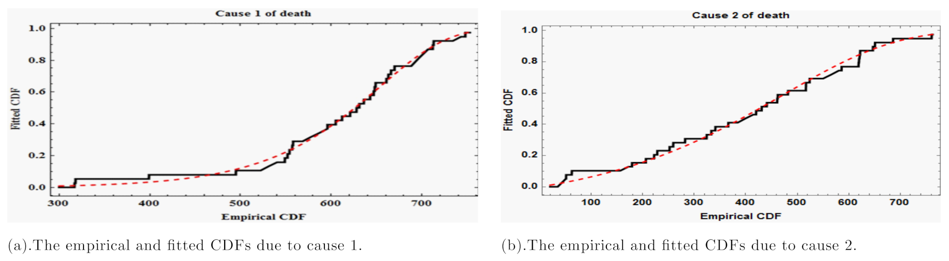
Based on these results, for the two causes of failure, one can say that at $5\%$ level of significance; the ${\chi }^2$ observed value is less than the ${\chi }^2$ tabulated value and the p-value is also quite large in this case. Thus, we can not reject H${}_0$ and the data set is fitted well with our model. In the same way, the computed K-S test statistics are higher than the critical value for the K-S test statistic. Additionally, as we can see, the p-values for the K-S test statistics for the Gompertz distribution are higher than the significance level (0.05), indicating that the Gompertz model generally well fits the previous real data. For further clarification, we provided Figure 1, which contains both fitted and empirical CDFs of Gompertz distribution based on the two causes (Figure 1a,b), computed at the estimated parameters. The figures show that the fitted distribution and empirical distribution are very similar. As a result, the Gompertz model provides an excellent fit to the provided data set in each scenario that results in death.

By using the censoring scheme $R_1=R_2=$···$=R_{24}=2,R_{25}=4$ and an ideal total test time $T=550$, we generate an adaptive progressively Type II censored sample of size $m=25$ from the complete data. The generated data is obtained as:

(40, 2), (42,2), (51, 2), (62,2), (179, 2), (206, 2), (222, 2), (228, 2), (252, 2), (259, 2), (282, 2), (317, 1), (318, 1), (324, 2), (341, 2), (366, 2), (385, 2), (399, 1), (461, 2), (517, 2), (549, 1), (557, 1), (586, 1), (636, 1), (649, 1).

From the above generated data, we observed $m_1=8$ failure due to cause 1, $m_2=17$ failures due to cause 2 and only 21 observed failures ($J=21$) were observed before time $T=550$. Thus, we have $R=(2^{21},0^3,10)$. Here, this sample will be utilized to perform numerical calculations on the results obtained through theoretical in earlier sections.

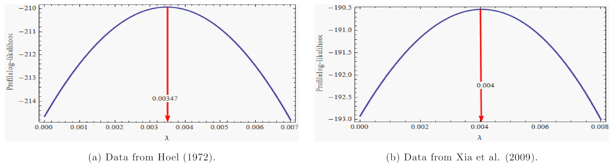
The iteration method and SEM algorithm, which are both covered in Section 3 and Section 4, are used to calculate the MLE of unknown parameters. Based on Hoel’data, we plot the profile log-likelihood function (13) before calculating the MLEs, see Figure 2a. From this figure, it can be seen that the profile log-likelihood function is unimodal with the mode falling between 0.003 and 0.004. It indicates that the MLE of $\lambda$ is unique.

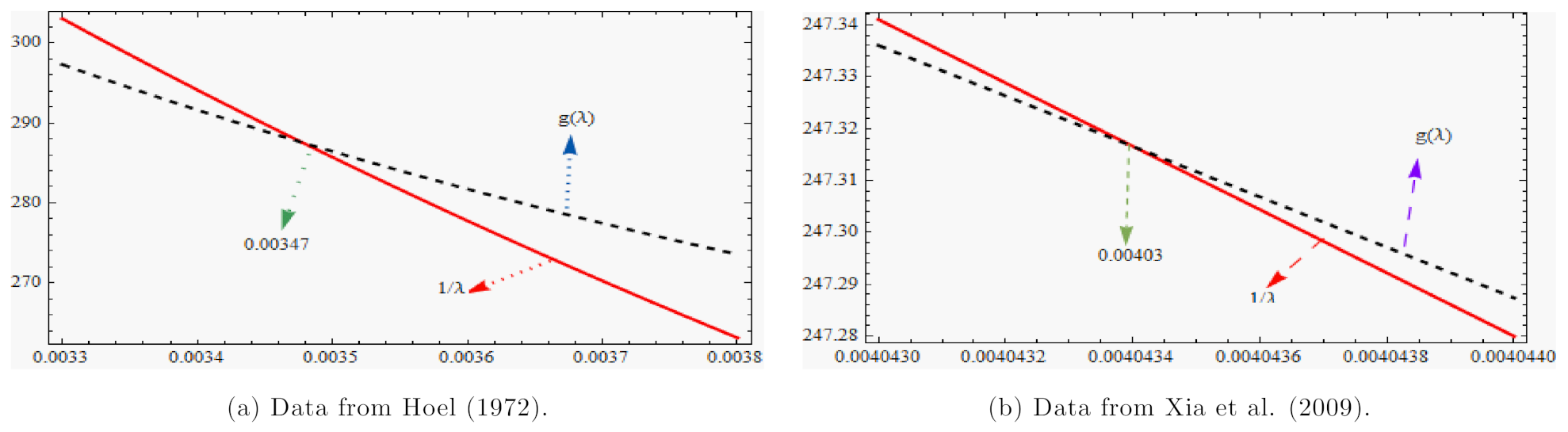
Additionally, a graphical technique developed by [43] is used to calculate the MLE of the shape parameter $\lambda$. Figure 3a shows the curves of ($\frac{1}{\lambda }$) and $g\left(\lambda \right)$ based on Hoel [56] data. According to Figure 3a, the intersection of the two functions $\frac{1}{\lambda }$ and $g\left(\lambda \right)$ is roughly at 0.00347. Therefore, to begin the iteration to determine the MLE of $\lambda$, we suggest choosing $\lambda =0.00347$ as the initial value, and stopping the process when $\left|{\lambda }^{(s+1)}-{\lambda }^{\left(s\right)}\right|<{10}^{-6}$. The MLEs of ${\theta }_1$, ${\theta }_2$, and $S\left(t\right)$ are computed based on NR method using the estimated initial value of $\lambda$, and the results are presented in

Table 2. Point estimate and standard error (SE) of ${\theta }_1$, ${\theta }_2$, $\lambda$ and S(t) for data from Hoel (1972).

		${\mathit{\theta }}_1$		${\mathit{\theta }}_2$		$\mathit{\lambda }$		S$(\mathit{t}=500)$
Method		Estimate	SE	Estimate	SE	Estimate	SE	Estimate	SE
NR		0.000117	2.38 × 10${}^{-6}$	0.000248	4.36 × 10${}^{-6}$	0.00348	0.000044	0.61112	0.002411
SEM		0.000160	2.32 × 10${}^{-6}$	0.000165	2.38 × 10${}^{-6}$	0.003941	0.000016	0.607149	0.001885
MCMC	SEL	0.000124	2.33 × 10${}^{-6}$	0.000264	4.10 × 10${}^{-6}$	0.00338	0.000037	0.614227	0.002959
	LINEX
	$c=-{10}^3$	0.000126		0.000269		0.003838		0.875585
	$c=+{10}^3$	0.000123		0.000259		0.002973		0.221293

along with the estimated standard errors. The reliability function $S\left(t\right)$ is computed at time $t=500$.

Next, we use the SEM method created in Section 3.2 to compute the MLEs of ${\theta }_1$, ${\theta }_2$, $\lambda$ and $S\left(t\right)$. For the SEM algorithm, the associated MLEs’ initial values of ${\theta }_1$, ${\theta }_2$ and $\lambda$ are established using the NR approach and $K=5100$ is assumed to be the number of SEM cycles. The first 100 cycles are employed as a burn-in period, and the following 5000 cycles are averaged to estimate the unknown parameters ${\theta }_1$, ${\theta }_2$, $\lambda$, and $S\left(t\right)$. 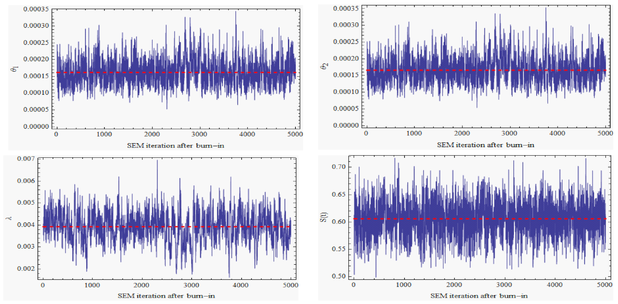The trace plots of these parameters against the SEM cycles are displayed in Figure 4. In this figure, the red horizontal lines represent the SEM cycles, and the parameter values bounce around them without exhibiting an upward or downward trend. This signifies that a stationary distribution for the Markov Chain {${\vartheta }^{\left(s\right)}$} has been reached. To approach the MLE, the average of the sequence {${\vartheta }^{\left(s\right)}$} would be sufficient. The computed and reported standard errors (SEs) for the MLEs derived using the SEM technique are shown also in Table 2. Using both the NR and the SEM techniques, the asymptotic 95% confidence intervals of ${\theta }_1$, ${\theta }_2$, $\lambda$, and $S\left(t\right)$ are computed, and the results are presented in

Table 3. Point and interval estimates of ${\theta }_1$, ${\theta }_2$, $\lambda$ and S(t) for the data from Hoel (1972).

	${\mathit{\theta }}_1$	${\mathit{\theta }}_2$	$\mathit{\lambda }$	S$(\mathit{t}=500)$
NR	(3.2 × 10${}^{-7}$, 0.000331)	(0.000035, 0.000462)	(0.001298, 0.005656)	(0.492959, 0.729277)
SEM	(0.000064, 0.000257)	(0.000066, 0.000264)	(0.002998, 0.004884)	(0.513890, 0.700407)
Boot-p	(0.0000221, 0.000096)	(0.000017, 0.000113)	(0.002673, 0.006567)	(0.774804, 0.875795)
Boot-t	(0.000102, 0.000116)	(0.000169, 0.000237)	(0.003434, 0.003580)	(0.619715, 0.629505)
MCMC	(0.000041, 0.000268)	(0.000108, 0.000501)	(0.001640, 0.005303)	(0.454243, 0.752024)

. Furthermore, the results of the computation of the 95% confidence intervals using the Boot-p and Boot-t with $B=1000$ bootstrap replications were also reported in Table 3.

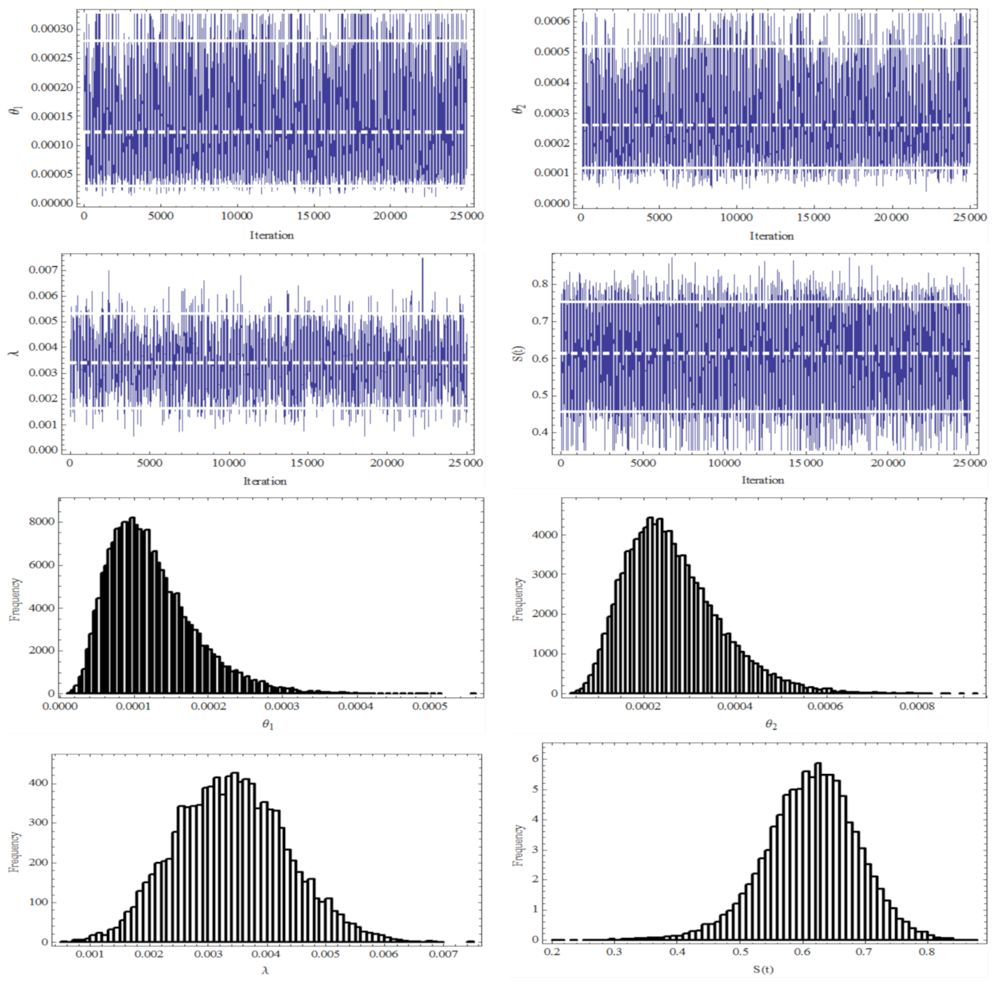
The Bayes estimates of ${\theta }_1$, ${\theta }_2$, $\lambda$, and $S(t=500)$ versus the SE and LINEX loss functions will now be calculated using the MCMC samples. Since we don’t know anything about the unknown parameters beforehand, we consider their noninformative gamma priors to be $a_i=b_i=0,i=1,2,3$. Nobody is not aware of the fact that for the LINEX loss function, $c>0$ implies that overestimation results in more penalty than underestimation and the converse is true for $c<0$. Additionally, the LINEX loss function becomes symmetric for c near zero and behaves similar to the SE loss function.

When the LINEX loss function is taken into consideration, Bayes estimates are generated for two alternative values of c, where $c=\pm {10}^3$. As was mentioned earlier in Section 5, the posterior analysis was conducted using a hybrid technique that included the Gibbs chain and Metropolis-Hastings. In order to run the MCMC sampler algorithm, the initial values for the three parameters ${\theta }_1$, ${\theta }_2$ and $\lambda$ were assumed to be their MLEs. With $N=30,000$ samples and the first $M=5000$ iterations serving as the burn-in period, we generate the Markov chain samples. The trace plots of the $25,000$ MCMC outputs for the posterior distribution of ${\theta }_1$, ${\theta }_2$, $\lambda$, and $S\left(t\right)$ are shown in Figure 5 (first row) to verify the MCMC method’s convergence. Also, Figure 5 displays histogram plots (second row) of the samples that we generated using the M-H algorithm for ${\theta }_1$, ${\theta }_2$, $\lambda$, and $S\left(t\right)$. It is clear that the MCMC method converges extremely effectively. In Table 2 and Table 3, point Bayes estimates for ${\theta }_1$, ${\theta }_2$, $\lambda$, and $S\left(t\right)$ are produced together with the corresponding 95% credible ranges. The estimated standard errors of the Bayes estimates are also calculated and are shown in Table 2.

6.2. Application to Breaking Strengths of Jute Fibres

Jute fibers contain a wide range of applications and become one of the most important fibers in the manufacture of bio-compounds. For instance, jute fibers are mainly used in the textile industry, where they are used to make clothes, ropes, bed covers, bags, shoelaces, etc. To a large extent, jute fibers also made their way into the automotive sector, where it is used to make cup holders, various parts of the instrument cluster, and door panels. According to a real-world data set published by Xia et al. [57], two different gauge lengths are what lead to the breaking strengths failure data of jute fiber. We denote ${\delta }_i=1$ if the breaking strengths of jute fiber of gauge length 10 mm and ${\delta }_i=2$ if the the breaking strengths of jute fiber of gauge length 20 mm. The breaking strengths of jute fibres at 10 mm, and 20 mm gauge lengths are provided in

Table 4. Breaking strengths of jute fiber under different gauge length from Xia et al. (2009).

Cause 1: Data with gauge length 10 mm
$43.93$	$50.16$	$101.15$	$123.06$	$108.94$	$141.38$	$151.48$	$163.40$	$177.25$	$183.16$
$212.13$	$257.44$	$262.90$	$291.27$	$303.90$	$323.83$	$353.24$	$376.42$	$383.43$	$422.11$
$506.60$	$530.55$	$590.48$	$637.66$	$671.49$	$693.73$	$700.74$	$704.66$	$727.23$	$778.17$
Cause 2: Data with gauge length 20 mm
$36.75$	$45.58$	$48.01$	$71.46$	$83.55$	$99.72$	$113.85$	$116.99$	$119.86$	$145.96$
$166.49$	$187.13$	$187.85$	$200.16$	$244.53$	$284.64$	$350.70$	$375.81$	$419.02$	$456.60$
$547.44$	$578.62$	$581.60$	$585.57$	$594.29$	$662.66$	$688.16$	$707.36$	$756.70$	$765.14$

. These two independent data sets representing two groups of breaking strengths samples as competing risks data, say cause 1 and cause 2, respectively.

Before processing, it was determined whether or not these data sets could be analyzed using the Gompertz distributions. Let random variables $X_1$ and $X_2$ be breaking strengths of jute fiber of gauge length 10 mm and 20 mm, respectively. Based on the MLEs via NR method, we first obtain the K-S with the corresponding p-values between the fitted distribution and the empirical CDF for two random variables $X_1$ and $X_2$.

Table 5. The test statistics for Chi-square (${\chi }^2$) and Kolmogorov-Smirnov (K-S) from Xia et al. (2009).

Data	($\widehat{\mathit{\theta }},\widehat{\mathit{\lambda }}$)	${\mathit{\chi }}^2$ (Observed)	${\mathit{\chi }}^2$ (Tabulated)	p-Value	K-S	p-Value
Cause 1	(0.00118, 0.00273)	7.76162	11.0705	0.1699	0.1020	0.9138
Cause 2	(0.00158, 0.00208)	5.47388	11.0705	0.3608	0.1426	0.5753

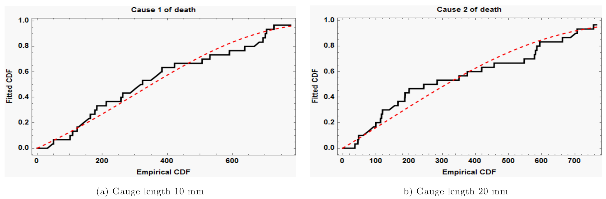
summarizes the results. The results do not allow us to reject the null hypothesis but force us to accept that the data comes from the Gompertz distribution. This is done for both cause 1 and cause 2. Figure 6 displays the fitted and empirical distribution functions. The two distributions for the two random variables $X_1$ and $X_2$ are a reasonably close match.

The previous data set was utilized in this illustration to simulate an adaptive progressive Type-II censored sample with $m=25$, ideal total test time $T=350$, and a progressive censoring scheme $R=({\left(3,1,0\right)}^8,3).$

For clarity, ${\left(3,1,0\right)}^2$ is given as a short form of $(3,1,0,3,1,0)$. Thus, the observed adaptive progressive Type-II censored sample of size m from the original complete sample of size $n=60$ is

(36.75, 2), (43.93, 1), (45.58, 2), (48.01, 2), (50.16, 1), (71.46, 2), (83.55, 2), (99.72, 2), (108.94, 1), (113.85, 2), (116.99, 2), (119.86, 2), (151.48, 1), (163.4, 1), (177.25, 1), (183.16, 1), (187.13, 2), (200.16, 2), (212.13, 1), (284.64, 2), (323.83, 1), (350.7, 2), (353.24, 1), (375.81, 2), (383.43, 1).

Here, $m_1=11$ and $m_2=14$, and $J=21$. Thus, we have $R=({\left(3,1,0\right)}^7,0^3,7)$. To find an initial guess of $\lambda$, we display the profile log-likelihood function of in Figure 2 to determine an initial guess of, and it is obvious that the profile log-likelihood is a unimodal function with a mode close to $0.004$. Furthermore, the position at which the two functions $\frac{1}{\lambda }$ and $g\left(\lambda \right)$ overlap in Figure 3b is quite close to $0.00403$. Then, according to Figure 2 and Figure 3, the initial value of $\lambda$ can be thought of as $0.004$. 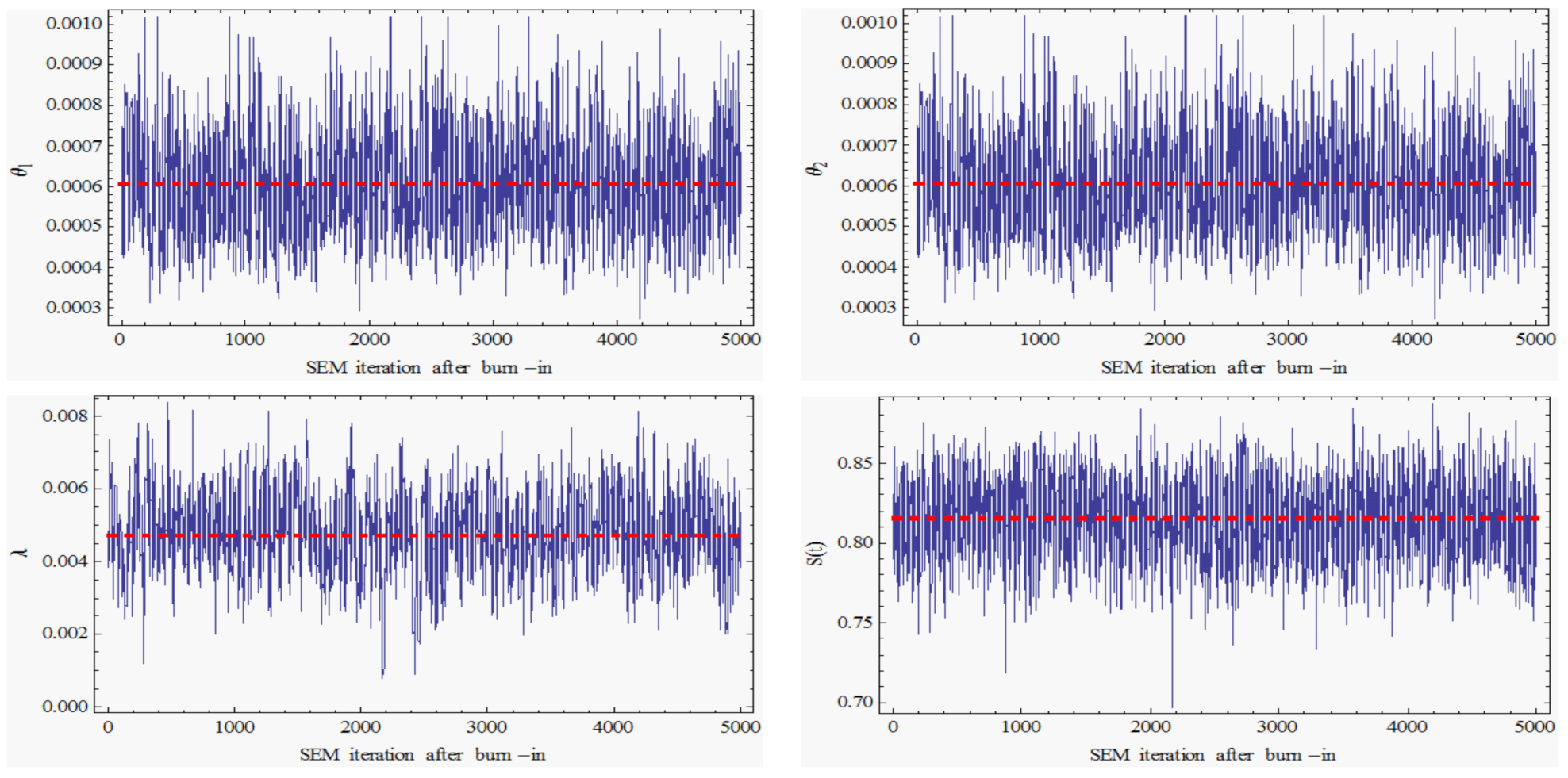The MLEs of ${\theta }_1$, ${\theta }_2$, $\lambda$, and $S\left(t\right)$ are obtained via both NR method and SEM algorithm with $t=125$. For the SEM algorithm, we used 5100 iterations and the first 100 iterations were used as burn-in. The trace graphs of these parameters versus the SEM cycles are shown in Figure 7. The average of the iterations after the burn-in should be used to estimate the parameters because Figure 7 indicates that SEM iterations have converged to a density function.

Table 6. ML and Bayes estimates of ${\theta }_1$, ${\theta }_2$, $\lambda$, and S(t) for Xia et al. (2009) data.

		MLE		MCMC
		NR	SEL	SEL	LINEX
Parameter	Criteria				$\mathit{c}=-1000$	$\mathit{c}=1000$
${\theta }_1$	Estimate	0.00058	0.000605	0.00081	0.00087	0.00075
	SE	0.501$\times {10}^{-4}$	0.353$\times {10}^{-4}$	0.686$\times {10}^{-4}$
${\theta }_2$	Estimate	0.00074	0.000605	0.00102	0.00111	0.00095
	SE	0.604$\times {10}^{-4}$	0.353$\times {10}^{-4}$	0.809$\times {10}^{-4}$
$\lambda$	Estimate	0.00404	0.004713	0.00215	0.00457	0.00092
	SE	0.359$\times {10}^{-3}$	0.153$\times {10}^{-3}$	0.411$\times {10}^{-3}$
$S(t=125)$	Estimate	0.80644	0.815362	0.77626	0.93759	0.57593
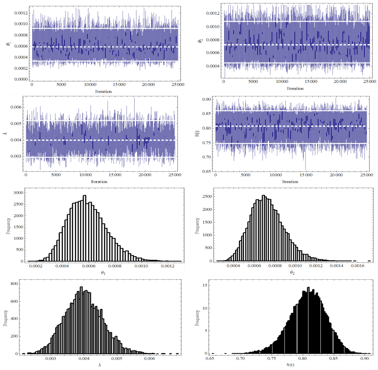
	SE	0.948$\times {10}^{-2}$	0.711$\times {10}^{-2}$	1.085$\times {10}^{-2}$

reports the MLEs with the NR and SEM algorithm of size 5000. Using noninformative gamma priors, Table 6 also includes the Bayes estimates of ${\theta }_1$, ${\theta }_2$, $\lambda$, and $S\left(t\right)$ with respect to the squared error (SE) loss function and the LINEX with $c=\pm {10}^3$. The trace plots and the histograms of the MCMC outputs of ${\theta }_1$, ${\theta }_2$, $\lambda$, and $S\left(t\right)$ based are represented in Figure 8. It is evident that from Figure 8, the MCMC procedure converges very well. Finally, the 95% asymptotic confidence intervals, bootstrap confidence intervals (Boot-p and Boot-t), and Bayes credible intervals for all parameters ${\theta }_1$, ${\theta }_2$, $\lambda$, and $S\left(t\right)$ are tabulated in

Table 7. 95% confidence intervals of ${\theta }_1,{\theta }_2,\lambda$, and S(t) for Xia et al. (2009) data.

		MLE		Bootstrap		Bayes
	95% CIs	NR	SEL	Boot-p	Boot-t
${\theta }_1$	Lower	0.00009	0.00025	0.00003	0.00032	0.00028
	Upper =	0.00117	0.00096	0.00068	0.00060	0.00159
	Length	0.00108	0.00071	0.00065	0.00038	0.00131
${\theta }_2$	Lower	0.00015	0.00025	0.00009	0.00008	0.00038
	Upper	0.00133	0.00096	0.00101	0.00078	0.00192
	Length	0.00118	0.00071	0.00092	0.00070	0.00154
$\lambda$	Lower	0.00052	0.00304	0.00283	0.00376	0.7$\times {10}^{-9}$
	Upper	0.00756	0.00639	0.00757	0.00472	0.00643
	Length	0.00704	0.00335	0.00474	0.00096	0.00643
S$(t=125)$	Lower	0.71355	0.74292	0.82547	0.81030	0.66687
	Upper	0.89933	0.88780	0.92886	0.85015	0.87576
	Length	0.18578	0.14488	0.10339	0.03985	0.20889

.

It is clear that the MCMC technique is better than the ML method via NR or SEM algorithm in respect of estimated standard error. Further, it is observed from Table 7 that the Boot-t intervals have shorter lengths than other intervals.

As can be seen in this previous examples, the outcomes of all estimates are similar. It should be noted that the MLEs produced by the SEM algorithm have the lowest standard errors. As a result, the performance of ML estimates acquired using the SEM algorithm is often superior to that of estimates obtained using the NR and MCMC methods with noninformative priors. We must provide numerical simulation to compare all methods accurately, clearly and objectively.

7. Simulation Study

In this section, we conduct a simulation analysis to evaluate the effectiveness of several estimation approaches for the unknwon parameters and reliability function covered in the preceding sections. We create adaptive Type-II progressive censored samples with competing risks from the Gompertz models by employing the algorithm described in Section 2 for specific total sample sizes $n=(30,60,80)$, failure sample sizes $m=(15,25,40,50,60)$, and censoring schemes. The true values of ${\theta }_1$, ${\theta }_2$ and $\lambda$ are assumed to be 0.05, 0.06, and 1.8, respectively. To create the appropriate samples, the progressive censoring schemes listed below are taken into account:

Scheme I: $R_1=n-m$ and $R_2=$···$=R_m=0$,

Scheme II: $R_1=R_2=$···$=R_{n-m}=1$ and $R_{n-m+1}=$···$=R_m=0,$

Scheme III: $R_1=R_2=$···$=R_{m-1}=0$ and $R_m=n-m$.

It should be noted that the first scheme is the left censoring scheme, where $n-m$ units are taken from the test at the time of the mth failure, the second scheme is the usual Type II progressive censoring scheme, and the third scheme is the Type II censoring scheme. Using the NR and SEM algorithm approaches, we compute MLEs of unknown parameters ${\theta }_1$, ${\theta }_2$, $\lambda$ as well as reliability function $S(t=0.9)$ based on generated data. We use the parameters’ true values as starting points for the SEM algorithm. Additionally, we perform the iterative procedure up to $K=1100$ iterations with $K_0=100$ serving as the burn-in sample in order to apply the SEM algorithm. We utilize the NMaximize command of the Mathematica 11 package to solve the nonlinear equations and obtain the MLEs of the parameters. Under the SE and LINEX loss functions, the gamma prior distributions are used to obtain the Bayes estimates of unknown parameters. There are two distinct priors considered. First, we examine the non-informative priors for the three parameters ${\theta }_1$, ${\theta }_2$, and $\lambda$. In this case, we choose hyper-parameters such that $a_i=b_i=0; i=1,2,3$. It is instructive to use a second prior in which the hyper-parameters are chosen so that the prior expectations equal the values of the corresponding true parameters, i.e., $a_1=1$, $a_2=3$, $a_3=9$, and $b_1=20, b_2=50, b_3=5$. This helps us to see how much does the informative prior effect contributes to the results obtained based on observed data. Additionally, when computing the Bayes estimates with regard to the LINEX loss function, we assume $c=-2.0$ and $2.0$, which, respectively, give more weight to underestimation and overestimation. These calculations are based on 10000 MCMC samples using Gibbs within the Metropolis method.

The accuracy of the point estimates (ML and Bayes) is compared against the bias and squared error values (MSE) in these settings. When evaluating the various interval estimations, we take into account the average interval lengths and the average interval coverage percentages (CPs). The scheme with the lowest mean squared error (MSE) of the estimator is considered to be the best one. In

Table 8. Average values of the biases (first row) and MSEs (second row) for MLEs and Bayes estimators of ${\theta }_1$ under informative prior (IP) and noninformative (NIP) prior and different censoring schemes, when (${\theta }_1$, ${\theta }_2$, $\lambda$) = (0.05, 0.06, 1.8).

$\mathit{T}=0.8$			MLEs		SEL		LINEX
							$\mathbf{c}=-\mathbf{2}$		$\mathbf{c}=\mathbf{2}$
($\mathit{n},\mathit{m}$)	Sc.	Statistic	NR	SEM	NIP	IP	NIP	IP	NIP	IP
(30, 15)	I	Bias	0.002981	0.003561	0.025490	0.004065	0.030289	0.005110	0.021610	0.003089
		MSE	0.001720	0.001108	0.004806	0.000670	0.006040	0.000720	0.003937	0.000627
	II	Bias	−0.001878	−0.004675	0.038669	0.002392	0.043224	0.003140	0.034630	0.001778
		MSE	0.001350	0.000794	0.005859	0.000471	0.006710	0.000497	0.005152	0.000453
	III	Bias	−0.002942	−0.008842	0.034542	0.000080	0.038906	0.000830	0.030680	−0.000636
		MSE	0.001410	0.000980	0.005252	0.000438	0.006036	0.000459	0.004605	0.000421
(30,25	I	Bias	−0.000462	0.004444	0.010035	0.002213	0.011624	0.002890	0.008610	0.001561
		MSE	0.000930	0.000936	0.001511	0.000475	0.001704	0.000498	0.001360	0.000454
	II	Bias	−0.000462	0.004444	0.009409	0.002382	0.010883	0.003050	0.008070	0.001745
		MSE	0.000930	0.000736	0.001336	0.000466	0.001488	0.000488	0.001214	0.000447
	III	Bias	−0.000889	0.002960	0.012998	0.001969	0.015003	0.002630	0.011220	0.001337
		MSE	0.000910	0.000823	0.001885	0.000428	0.002158	0.000448	0.001668	0.000410
(60, 40)	I	Bias	0.000125	0.001179	0.006245	0.002090	0.006959	0.002540	0.005560	0.001651
		MSE	0.000540	0.000421	0.000798	0.000353	0.000846	0.000364	0.000755	0.000342
	II	Bias	0.000029	−0.001936	0.008095	0.002117	0.008966	0.002540	0.007270	0.001703
		MSE	0.000550	0.000423	0.000860	0.000298	0.000921	0.000307	0.000806	0.000289
	III	Bias	−0.000600	−0.002180	0.007837	0.000995	0.008724	0.001400	0.007000	0.000597
		MSE	0.000560	0.000492	0.000940	0.000281	0.001008	0.000289	0.000880	0.000274
(60, 50)	I	Bias	−0.000097	0.002850	0.004633	0.001995	0.005155	0.002370	0.004130	0.001635
		MSE	0.000400	0.000383	0.000488	0.000286	0.000508	0.000294	0.000470	0.000279
	II	Bias	−0.000112	0.003127	0.004533	0.001907	0.005034	0.002260	0.004050	0.001558
		MSE	0.000410	0.000386	0.000478	0.000283	0.000497	0.000291	0.000462	0.000276
	III	Bias	−0.000897	0.001976	0.004597	0.001150	0.005167	0.001520	0.004050	0.000792
		MSE	0.000430	0.000416	0.000550	0.000275	0.000574	0.000282	0.000528	0.000268
(80, 65)	I	Bias	−0.000765	0.001301	0.002684	0.001008	0.003051	0.001290	0.002330	0.000729
		MSE	0.000310	0.000272	0.000356	0.000238	0.000367	0.000243	0.000347	0.000234
	II	Bias	−0.001152	0.001403	0.002470	0.000916	0.002827	0.001190	0.002120	0.000645
		MSE	0.000300	0.000281	0.000335	0.000220	0.000344	0.000224	0.000327	0.000216
	III	Bias	0.000004	0.001334	0.004086	0.001664	0.004498	0.001960	0.003690	0.001375
		MSE	0.000350	0.000322	0.000418	0.000248	0.000432	0.000254	0.000405	0.000243
$T=1.5$
(30, 15)	I	Bias	0.001502	−0.000309	0.023855	0.003896	0.028537	0.004930	0.020060	0.002928
		MSE	0.001520	0.000938	0.004400	0.000640	0.005539	0.000687	0.003602	0.000599
	II	Bias	−0.000454	−0.004452	0.038777	0.001966	0.043437	0.002770	0.03466	0.001204
		MSE	0.001660	0.000899	0.005861	0.000510	0.006754	0.000538	0.005126	0.000485
	III	Bias	−0.000171	−0.008871	0.038645	0.002335	0.043311	0.003140	0.034520	0.001566
		MSE	0.001670	0.000928	0.005928	0.000506	0.006835	0.000534	0.005179	0.000481
(30, 25)	I	Bias	−0.001569	0.004109	0.008676	0.001601	0.010150	0.002270	0.00734	0.000963
		MSE	0.000800	0.000831	0.001289	0.000432	0.001441	0.000452	0.001166	0.000414
	II	Bias	0.002109	0.006579	0.012561	0.003898	0.014080	0.004580	0.011180	0.003240
		MSE	0.000900	0.000877	0.001694	0.000493	0.001874	0.000519	0.001545	0.000471
	III	Bias	−0.000291	0.003273	0.013609	0.002118	0.015607	0.002780	0.011840	0.001485
		MSE	0.000870	0.000843	0.001761	0.000418	0.002010	0.000438	0.001563	0.000401
							$\mathbf{c}=-\mathbf{2}$		$\mathbf{c}=\mathbf{2}$
($\mathbf{n},\mathbf{m}$)	Sc.	Statistic	NR	SEM	NIP	IP	NIP	IP	NIP	IP
(60, 40)	I	Bias	0.000207	0.003018	0.006231	0.002102	0.006949	0.002560	0.005550	0.001661
		MSE	0.000570	0.000457	0.000735	0.000367	0.000775	0.000379	0.000700	0.000356
	II	Bias	0.000328	0.001248	0.005431	0.002315	0.005991	0.002700	0.004890	0.001940
		MSE	0.000480	0.000396	0.000593	0.000332	0.000619	0.000342	0.000570	0.000323
	III	Bias	0.000520	−0.000314	0.008870	0.002348	0.009780	0.002780	0.008010	0.001931
		MSE	0.000560	0.000501	0.000936	0.000303	0.001006	0.000313	0.000874	0.000294
(60, 50)	I	Bias	−0.000824	0.001667	0.003893	0.001264	0.004406	0.001630	0.003400	0.000909
		MSE	0.000420	0.000393	0.000506	0.000297	0.000526	0.000305	0.000488	0.000290
	II	Bias	0.000096	0.003317	0.004441	0.001987	0.004923	0.002340	0.003970	0.001642
		MSE	0.000400	0.000391	0.000485	0.000292	0.000503	0.000299	0.000468	0.000284
	III	Bias	0.000063	0.001939	0.005630	0.001700	0.006222	0.002070	0.005060	0.001336
		MSE	0.000480	0.000431	0.000665	0.000299	0.000699	0.000307	0.000633	0.000292
(80, 65)	I	Bias	0.000528	0.004156	0.004538	0.002114	0.004538	0.002410	0.003780	0.001826
		MSE	0.000320	0.000378	0.000390	0.000242	0.000390	0.000248	0.000366	0.000237
	II	Bias	0.000455	0.002182	0.003666	0.002010	0.004010	0.002280	0.003330	0.001741
		MSE	0.000310	0.000304	0.000357	0.000252	0.000367	0.000257	0.000347	0.000247
	III	Bias	0.000571	0.001527	0.004764	0.002124	0.005180	0.002420	0.004360	0.001832
		MSE	0.000310	0.000276	0.000380	0.000221	0.000393	0.000226	0.000368	0.000216

,

Table 9. Average values of the biases (first row) and MSEs (second row) for MLEs and Bayes estimators of ${\theta }_2$ under informative prior (IP) and noninformative (NIP) prior and different censoring schemes, when (${\theta }_1$, ${\theta }_2$, $\lambda$) = (0.05, 0.06, 1.8).

$\mathit{T}=0.8$			MLEs		SEL		LINEX
							$\mathbf{c}=-\mathbf{2}$		$\mathbf{c}=\mathbf{2}$
($\mathit{n},\mathit{m}$)	Sc.	Statistic	NR	SEM	NIP	IP	NIP	IP	NIP	IP
(30, 15)	I	Bias	0.004534	0.000118	0.032101	0.006139	0.038707	0.007582	0.026830	0.004795
		MSE	0.002550	0.001161	0.007320	0.000978	0.009418	0.001066	0.005856	0.000904
	II	Bias	−0.001875	−0.009407	0.044429	0.001195	0.050337	0.002212	0.039210	0.000230
		MSE	0.001970	0.001125	0.007628	0.000666	0.008862	0.000599	0.006612	0.000539
	III	Bias	−0.002673	−0.011689	0.042848	0.001497	0.048761	0.002515	0.037650	0.000531
		MSE	0.001950	0.001039	0.007093	0.000531	0.008272	0.000561	0.006131	0.000525
(30, 25)	I	Bias	0.000943	−0.006170	0.013889	0.004175	0.016145	0.005135	0.011890	0.003263
		MSE	0.001380	0.000908	0.002305	0.000731	0.002643	0.000774	0.002043	0.000693
	II	Bias	−0.000564	−0.006537	0.011685	0.003458	0.013696	0.004365	0.009890	0.002593
		MSE	0.001170	0.000803	0.001802	0.000630	0.002032	0.000664	0.001621	0.000599
	III	Bias	−0.001422	−0.008132	0.015044	0.001986	0.017736	0.002868	0.012700	0.001144
		MSE	0.001270	0.000929	0.002593	0.000501	0.002993	0.000531	0.002281	0.000514
(60, 40)	I	Bias	0.000053	−0.000055	0.007330	0.002424	0.008291	0.003033	0.006420	0.001834
		MSE	0.000750	0.000564	0.001068	0.000485	0.001136	0.000503	0.001006	0.000469
	II	Bias	−0.000804	−0.004245	0.008658	0.001822	0.009804	0.002385	0.007580	0.001275
		MSE	0.000720	0.000552	0.001108	0.000388	0.001194	0.000401	0.001032	0.000376
	III	Bias	0.000663	−0.004257	0.011041	0.002499	0.012307	0.003071	0.009860	0.001945
		MSE	0.000880	0.000531	0.001505	0.000447	0.001629	0.000463	0.001397	0.000433
(60, 50)	I	Bias	−0.000555	−0.003030	0.005074	0.002007	0.005775	0.002504	0.004400	0.001524
		MSE	0.000540	0.000428	0.000658	0.000387	0.000688	0.000399	0.000631	0.000376
	II	Bias	−0.000798	−0.004922	0.005835	0.001798	0.006614	0.002300	0.005090	0.001309
		MSE	0.000560	0.000435	0.000727	0.000363	0.000764	0.000374	0.000694	0.000353
	III	Bias	0.000044	−0.003623	0.006653	0.002339	0.007457	0.002848	0.005880	0.001843
		MSE	0.000660	0.000505	0.000846	0.000415	0.000889	0.000428	0.000806	0.000403
(80, 65)	I	Bias	−0.000375	−0.002775	0.003821	0.001828	0.004329	0.002220	0.003330	0.001444
		MSE	0.000420	0.000339	0.000482	0.000316	0.000499	0.000323	0.000467	0.000308
	II	Bias	−0.001150	−0.002500	0.003195	0.001370	0.003684	0.001747	0.002720	0.001001
		MSE	0.000410	0.000363	0.000465	0.000309	0.000479	0.000316	0.000453	0.000303
	III	Bias	−0.000066	−0.002956	0.004835	0.001940	0.005395	0.002340	0.004290	0.001548
		MSE	0.000460	0.000351	0.000554	0.000320	0.000575	0.000329	0.000535	0.000313
							$\mathbf{c}=-\mathbf{2}$		$\mathbf{c}=\mathbf{2}$
($\mathbf{n},\mathbf{m}$)	Sc.	Statistic	NR	SEM	NIP	IP	NIP	IP	NIP	IP
(30, 15)	I	Bias	−0.000278	−0.003966	0.025252	0.003203	0.031059	0.004534	0.020620	0.001962
		MSE	0.002000	0.001094	0.005445	0.000782	0.006937	0.000846	0.004426	0.000729
	II	Bias	0.000239	−0.005584	0.047790	0.003777	0.054031	0.004861	0.042300	0.002750
		MSE	0.002070	0.001206	0.007892	0.000638	0.009226	0.000659	0.006801	0.000596
	III	Bias	−0.001637	−0.012405	0.044407	0.002312	0.050426	0.003361	0.039120	0.001317
		MSE	0.001950	0.001185	0.007450	0.000612	0.008704	0.000650	0.006431	0.000579
(30, 25)	I	Bias	−0.002069	−0.006832	0.010128	0.001895	0.012099	0.002793	0.008360	0.001039
		MSE	0.001020	0.000777	0.001620	0.000563	0.001826	0.000592	0.001457	0.000537
	II	Bias	0.001919	−0.003387	0.014108	0.004506	0.016093	0.005423	0.012320	0.003632
		MSE	0.001110	0.000900	0.001847	0.000625	0.002070	0.000661	0.001666	0.000584
	III	Bias	0.000437	0.008593	0.016206	0.002677	0.018162	0.003799	0.014430	0.001619
		MSE	0.001270	0.000855	0.002742	0.000566	0.003047	0.000605	0.002486	0.000533
(60, 40)	I	Bias	0.000595	−0.002414	0.007875	0.003077	0.008855	0.003699	0.006940	0.002474
		MSE	0.000760	0.000538	0.000992	0.000479	0.001053	0.000498	0.000937	0.000462
	II	Bias	0.000005	0.000151	0.006088	0.002483	0.006831	0.002993	0.005370	0.001986
		MSE	0.000620	0.000567	0.000774	0.000429	0.000812	0.000443	0.000740	0.000416
	III	Bias	0.000468	0.002082	0.010422	0.002286	0.011337	0.003004	0.009550	0.001594
		MSE	0.000810	0.000587	0.001306	0.000418	0.001384	0.000437	0.001236	0.000402
(60, 50)	I	Bias	−0.001201	−0.004170	0.004444	0.001394	0.005137	0.001886	0.00378	0.000916
		MSE	0.000570	0.000467	0.000684	0.000398	0.000715	0.000410	0.000657	0.000388
	II	Bias	0.000258	−0.002340	0.005442	0.002583	0.006101	0.003065	0.004810	0.002114
		MSE	0.000560	0.000493	0.000671	0.000408	0.000701	0.000420	0.000645	0.000396
	III	Bias	0.000398	0.004119	0.006259	0.001905	0.006843	0.002532	0.005690	0.001299
		MSE	0.000560	0.000476	0.000720	0.000355	0.000747	0.000369	0.000694	0.000349
(80, 65)	I	Bias	0.000608	−0.001654	0.004997	0.002535	0.005520	0.002935	0.00449	0.002144
		MSE	0.000450	0.000360	0.000539	0.000347	0.000559	0.000356	0.000521	0.000338
	II	Bias	0.000155	−0.002129	0.003989	0.002062	0.004448	0.002427	0.003540	0.001705
		MSE	0.000390	0.000342	0.000444	0.000306	0.000458	0.000314	0.000431	0.000300
	III	Bias	0.000294	0.003268	0.004725	0.001756	0.005144	0.002254	0.004320	0.001270
		MSE	0.000510	0.000371	0.000623	0.000351	0.000639	0.000366	0.000607	0.000345

,

Table 10. Average values of the biases (first row) and MSEs (second row) for MLEs and Bayes estimators of $\lambda$ under informative prior (IP) and noninformative (NIP) prior and different censoring schemes, when (${\theta }_1$, ${\theta }_2$, $\lambda$) = (0.05, 0.06, 1.8).

$\mathit{T}=0.8$			MLEs		SEL		LINEX
							$\mathbf{c}=-\mathbf{2}$		$\mathbf{c}=\mathbf{2}$
($\mathit{n},\mathit{m}$)	Sc.	Statistic	NR	SEM	NIP	IP	NIP	IP	NIP	IP
(30, 15)	I	Bias	0.179162	0.114900	0.030558	0.082385	0.303908	0.204413	−0.234290	−0.028933
		MSE	0.335900	0.170286	0.377886	0.074067	0.574149	0.126221	0.381641	0.055574
	II	Bias	0.328080	0.375084	−0.141489	0.113266	0.590084	0.310275	−0.709730	−0.052580
		MSE	0.762950	0.456461	1.010090	0.075167	1.728490	0.182796	1.118150	0.049245
	III	Bias	0.347467	0.426425	−0.114099	0.118621	0.609937	0.314043	−0.687460	−0.046693
		MSE	0.751880	0.516007	0.963829	0.075534	1.711310	0.183035	1.079190	0.068319
(30, 25)	I	Bias	0.136497	0.129389	0.063529	0.075185	0.212406	0.164106	−0.082030	−0.009066
		MSE	0.179150	0.155368	0.180600	0.066676	0.245054	0.097923	0.168143	0.0529610
	II	Bias	0.159588	0.136501	0.081028	0.077393	0.251696	0.174322	−0.082940	−0.012808
		MSE	0.215720	0.171223	0.207620	0.069393	0.320055	0.108527	0.171066	0.052445
	III	Bias	0.176044	0.186346	0.068027	0.091451	0.286579	0.202572	−0.143810	−0.011334
		MSE	0.25455	0.201025	0.266055	0.074288	0.386459	0.119440	0.262045	0.066133
(60, 40)	I	Bias	0.075532	0.045076	0.032702	0.048365	0.116705	0.109324	−0.049650	−0.010646
		MSE	0.101300	0.068181	0.103167	0.054086	0.124499	0.068957	0.096815	0.047279
	II	Bias	0.109760	0.144712	0.033570	0.062049	0.189716	0.155824	−0.118980	−0.026133
		MSE	0.159650	0.123332	0.167453	0.060592	0.218387	0.088728	0.170870	0.050997
	III	Bias	0.097088	0.128339	0.015668	0.053873	0.170958	0.146834	−0.136660	−0.033404
		MSE	0.181470	0.114536	0.197174	0.070262	0.241520	0.097903	0.206914	0.061001
							$\mathbf{c}=-\mathbf{2}$		$\mathbf{c}=\mathbf{2}$
($\mathbf{n},\mathbf{m}$)	Sc.	Statistic	NR	SEM	NIP	IP	NIP	IP	NIP	IP
(60, 50)	I	Bias	0.060359	0.050171	0.026613	0.036909	0.092867	0.087208	−0.038610	−0.012216
		MSE	0.073030	0.063848	0.072314	0.043333	0.085303	0.052852	0.068669	0.039243
	II	Bias	0.067231	0.045486	0.030182	0.038477	0.104362	0.093667	−0.042500	−0.015081
		MSE	0.087210	0.069006	0.084471	0.048072	0.105999	0.061242	0.075673	0.041768
	III	Bias	0.080867	0.078959	0.036217	0.050297	0.130202	0.116715	−0.054920	−0.013599
		MSE	0.102270	0.073716	0.104055	0.051560	0.128217	0.067004	0.098995	0.045397
(80, 65)	I	Bias	0.053679	0.047267	0.029130	0.036033	0.079363	0.076585	−0.020630	−0.003885
		MSE	0.058590	0.047796	0.057663	0.038898	0.066012	0.045663	0.054679	0.035593
	II	Bias	0.076784	0.055005	0.047702	0.050211	0.110015	0.098807	−0.013440	0.002782
		MSE	0.071040	0.055129	0.069185	0.043494	0.086902	0.055266	0.060348	0.037008
	III	Bias	0.054573	0.058394	0.021173	0.034586	0.093216	0.089135	−0.049360	−0.018463
		MSE	0.077890	0.056425	0.078481	0.045761	0.091760	0.055656	0.076184	0.042101
$T=1.5$
(30, 15)	I	Bias	0.206549	0.160738	0.060877	0.098353	0.336904	0.221013	−0.206350	−0.013571
		MSE	0.313720	0.199322	0.343209	0.076587	0.529587	0.132120	0.350884	0.055150
	II	Bias	0.314232	0.318476	−0.161213	0.110223	0.570395	0.306423	−0.733670	−0.055412
		MSE	0.697180	0.404996	0.940526	0.070720	1.605790	0.174945	1.092980	0.046494
	III	Bias	0.339302	0.504470	−0.128673	0.119982	0.601303	0.317356	−0.70398	−0.046703
		MSE	0.729550	0.595949	0.964092	0.072367	1.722960	0.180883	1.084490	0.058519
(30, 25)	I	Bias	0.140106	0.114795	0.068714	0.076818	0.218504	0.166279	−0.076300	−0.007634
		MSE	0.164300	0.136196	0.161795	0.060136	0.229124	0.091031	0.147194	0.046948
	II	Bias	0.097824	0.092587	0.024398	0.052923	0.163519	0.138061	−0.112640	−0.027771
		MSE	0.154350	0.135458	0.160605	0.060252	0.208122	0.085209	0.158088	0.051080
	III	Bias	0.151635	0.165738	0.046897	0.077384	0.203965	0.216469	−0.10682	−0.048438
		MSE	0.234990	0.173774	0.259561	0.069984	0.325633	0.126588	0.251630	0.056881
(60, 40)	I	Bias	0.074050	0.056077	0.030944	0.045080	0.115628	0.106147	−0.052120	−0.014060
		MSE	0.106400	0.078109	0.106168	0.055703	0.128169	0.070102	0.1001240	0.049318
	II	Bias	0.079631	0.050804	0.030725	0.045249	0.111146	0.104335	−0.049930	−0.012780
		MSE	0.103990	0.072658	0.101997	0.056509	0.122253	0.070709	0.095997	0.049923
	III	Bias	0.099133	0.093791	0.020545	0.058303	0.137385	0.176871	−0.09486	−0.051435
		MSE	0.180100	0.113124	0.193343	0.069540	0.224046	0.108907	0.194415	0.054740
(60, 50)	I	Bias	0.075059	0.068369	0.040881	0.049768	0.107687	0.101093	−0.024990	−0.000241
		MSE	0.079900	0.069132	0.078408	0.046899	0.093928	0.058240	0.072516	0.0412230
	II	Bias	0.060957	0.050443	0.028456	0.038583	0.092052	0.087899	−0.03426	−0.009645
		MSE	0.073100	0.067228	0.072418	0.044099	0.085076	0.053389	0.068388	0.039979
	III	Bias	0.067913	0.075543	0.022469	0.042707	0.092042	0.125652	−0.045770	−0.036378
		MSE	0.095070	0.074898	0.096293	0.048813	0.110104	0.068710	0.092914	0.043348
(80, 65)	I	Bias	0.037681	0.034209	0.011438	0.023248	0.061184	0.063595	−0.037780	−0.016424
		MSE	0.055620	0.046851	0.055698	0.037040	0.062062	0.042688	0.054527	0.034793
	II	Bias	0.040222	0.038361	0.015553	0.025146	0.062588	0.063666	−0.031000	−0.012852
		MSE	0.051240	0.046562	0.050909	0.035126	0.057127	0.040475	0.049360	0.032896
	III	Bias	0.063422	0.068207	0.028937	0.041414	0.083057	0.110367	−0.024220	−0.024855
		MSE	0.083810	0.059432	0.085214	0.046106	0.095322	0.063984	0.081438	0.043232

,

Table 11. Average values of the biases (first row) and MSEs (second row) for MLEs and Bayes estimators of S (t = 0.9) under informative prior (IP) and noninformative (NIP) prior and different censoring schemes, when (${\theta }_1$, ${\theta }_2$, $\lambda$) = (0.05, 0.06, 1.8).

$\mathit{T}=0.8$			MLEs		SEL		LINEX
							$\mathbf{c}=-\mathbf{2}$		$\mathbf{c}=\mathbf{2}$
($\mathit{n},\mathit{m}$)	Sc.	Statistic	NR	SEM	NIP	IP	NIP	IP	NIP	IP
(30, 15)	I	Bias	−0.002090	−0.000338	−0.023142	−0.006557	−0.015753	−0.001900	−0.030980	−0.011428
		MSE	0.007414	0.004756	0.009231	0.003450	0.008435	0.003259	0.010184	0.003696
	II	Bias	0.004043	0.013142	−0.021266	−0.004394	−0.015819	−0.000660	−0.026960	−0.008289
		MSE	0.004930	0.004468	0.005811	0.002811	0.005449	0.002674	0.006243	0.002985
	III	Bias	0.007852	0.017509	−0.017486	−0.001774	−0.012093	0.001900	−0.023130	−0.005612
		MSE	0.004684	0.004357	0.005424	0.002553	0.005110	0.002446	0.005806	0.002695
(30, 25)	I	Bias	0.003465	0.005372	−0.008718	−0.002165	−0.004163	0.001110	−0.013480	−0.005554
		MSE	0.004726	0.004015	0.005056	0.002561	0.004801	0.002483	0.005367	0.002665
	II	Bias	0.004467	0.004802	−0.007372	−0.001871	−0.003041	0.001270	−0.011890	−0.005112
		MSE	0.004292	0.003988	0.004473	0.002267	0.004269	0.002199	0.004724	0.002358
	III	Bias	0.006550	0.008857	−0.007711	−0.000177	−0.003260	0.002850	−0.012360	−0.003305
		MSE	0.004389	0.004108	0.004905	0.002203	0.004673	0.002153	0.005188	0.002275
(60, 40)	I	Bias	0.002860	0.001574	−0.004505	−0.000022	−0.001723	0.002210	−0.007370	−0.002309
		MSE	0.002833	0.002192	0.002976	0.001831	0.002887	0.001799	0.003084	0.001874
	II	Bias	0.001798	0.005486	−0.005777	−0.001623	−0.003344	0.000250	−0.008270	−0.003528
		MSE	0.002222	0.002123	0.002382	0.001378	0.002312	0.001354	0.002466	0.001411
	III	Bias	−0.000679	0.001804	−0.008379	−0.003608	−0.005913	−0.001720	−0.010910	−0.005531
		MSE	0.002212	0.002074	0.002440	0.001427	0.002355	0.001475	0.002539	0.001447
(60, 50)	I	Bias	0.002902	0.002082	−0.003065	−0.000088	−0.000801	0.001780	−0.005380	−0.001997
		MSE	0.002099	0.001801	0.002142	0.001457	0.002089	0.001436	0.002206	0.001486
	II	Bias	0.001276	0.001583	−0.004435	−0.00144	−0.002284	0.000350	−0.00663	−0.003259
		MSE	0.002037	0.001843	0.002055	0.001327	0.002004	0.001363	0.002116	0.001418
	III	Bias	0.003809	0.004571	−0.002515	0.000697	−0.000342	0.002450	−0.004740	−0.001088
		MSE	0.001997	0.001884	0.002071	0.001300	0.002027	0.001286	0.002127	0.001321
(80, 65)	I	Bias	0.002945	0.003065	−0.001454	0.000498	0.000288	0.002000	−0.003230	−0.001024
		MSE	0.001642	0.001368	0.001657	0.001212	0.001628	0.001199	0.001693	0.001229
	II	Bias	0.002547	0.001987	−0.001786	−0.000230	−0.000158	0.001170	−0.003440	−0.001651
		MSE	0.001524	0.001440	0.001549	0.001124	0.001526	0.001111	0.001579	0.001141
	III	Bias	0.001752	0.002747	−0.002839	−0.000345	−0.001188	0.001040	−0.004520	−0.001755
		MSE	0.001584	0.001495	0.001624	0.001127	0.001594	0.001115	0.001659	0.001144
$T=1.5$
(30, 15)	I	Bias	0.003401	0.009764	−0.017613	−0.003657	−0.010292	0.00093	−0.025400	−0.008463
		MSE	0.006736	0.004662	0.008248	0.003239	0.007561	0.003082	0.009091	0.003448
	II	Bias	−0.000683	0.007124	−0.025730	−0.008511	−0.020195	−0.00469	−0.031520	−0.012504
		MSE	0.005107	0.004430	0.005998	0.003180	0.005586	0.002995	0.006485	0.003406
	III	Bias	0.002465	0.013862	−0.022256	−0.006814	−0.016783	−0.003020	−0.027990	−0.01077
		MSE	0.005377	0.005081	0.006162	0.003072	0.005780	0.002906	0.006614	0.003278
(30, 25)	I	Bias	0.008027	0.006861	−0.004111	0.001712	0.000364	0.00494	−0.00879	−0.001627
		MSE	0.004137	0.003521	0.004318	0.002222	0.004130	0.002178	0.004559	0.002290
	II	Bias	−0.001135	−0.000542	−0.012432	−0.004362	−0.008092	−0.001190	−0.016950	−0.007640
		MSE	0.004231	0.003881	0.004644	0.002419	0.004388	0.002331	0.004950	0.002531
	III	Bias	0.003926	0.006532	−0.010595	−0.001434	−0.006078	0.001620	−0.015320	−0.004583
		MSE	0.003983	0.003761	0.004532	0.002072	0.004286	0.002017	0.004833	0.002148
(60, 40)	I	Bias	0.002488	0.001781	−0.004976	−0.000560	−0.002157	0.001700	−0.007880	−0.002868
		MSE	0.002864	0.002197	0.002960	0.001801	0.002867	0.001767	0.003072	0.001846
	II	Bias	0.000494	0.000402	−0.005088	−0.002108	−0.002903	−0.000270	−0.007320	−0.003984
		MSE	0.002192	0.002013	0.002234	0.001542	0.002173	0.001511	0.002306	0.001581
	III	Bias	−0.000679	0.001804	−0.008379	−0.003608	−0.005913	−0.001720	−0.010910	−0.005531
		MSE	0.002212	0.002074	0.002440	0.001427	0.002355	0.001475	0.002539	0.001447
(60, 50)	I	Bias	0.004606	0.004970	−0.001450	0.001426	0.000794	0.003290	−0.003750	−0.000478
		MSE	0.002255	0.001966	0.002284	0.001545	0.002237	0.001529	0.002342	0.001569
	II	Bias	0.001056	0.000651	−0.004177	−0.001441	−0.002065	0.000350	−0.006340	−0.003260
		MSE	0.002064	0.001948	0.002112	0.001463	0.002059	0.001438	0.002175	0.001496
	III	Bias	0.002684	0.003881	−0.003592	0.000237	−0.001424	0.001990	−0.005810	−0.001549
		MSE	0.002185	0.002029	0.002273	0.001418	0.002221	0.001401	0.002335	0.001442
							$\mathbf{c}=-\mathbf{2}$		$\mathbf{c}=\mathbf{2}$
($\mathbf{n},\mathbf{m}$)	Sc.	Statistic	NR	SEM	NIP	IP	NIP	IP	NIP	IP
(80, 65)	I	Bias	0.000684	0.000377	−0.003949	−0.001248	−0.002193	0.000260	−0.005740	−0.002783
		MSE	0.001703	0.001446	0.001745	0.001258	0.001707	0.001240	0.001791	0.001282
	II	Bias	0.000607	0.001458	−0.003276	−0.001182	−0.001687	0.000210	−0.004890	−0.002593
		MSE	0.001545	0.001456	0.001560	0.001198	0.001530	0.001181	0.001596	0.001219
	III	Bias	0.000937	0.001927	−0.003811	−0.000827	−0.002156	0.000570	−0.005500	−0.002242
		MSE	0.001478	0.001418	0.001519	0.001053	0.001488	0.001040	0.001557	0.001070

, we show the bias and MSEs of the proposed estimates of the unknown parameters and reliability function. The results are presented by considering two different values of $T$( $0.8$, $1.5$). By using NR, the SEM algorithm, bootstrap (Boot-p and Boot-t), and MCMC intervals (with non-informative prior (NIP) and informative prior (IP)), the average length (AV) and coverage probability (CP) of 95% asymptotic confidence are provided in

Table 12. 95% CI’s, average length (AL) and coverage percentage (CP) of approximate, Bayes and bootstrap confidence intervals of ${\theta }_1$ under informative prior (IP) and noninformative (NIP) prior, for different schemes with different values of n and m, when (${\theta }_1$, ${\theta }_2$, $\lambda$) =(0.05,0.06,1.8).

$\mathit{T}=0.8$		MLEs				MCMC Intervals				Bootstrap Intervals
		NR		SEM		NIP		IP		Boot-p		Boot-t
($\mathit{n},\mathit{m}$)	Sc.	AL	CP	AL	CP	AL	CP	AL	CP	AL	CP	AL	CP
(30, 15)	I	0.1938	0.950	0.1399	0.932	0.2019	0.917	0.1140	0.971	0.1986	0.891	0.2021	0.921
	II	0.1970	0.947	0.1380	0.888	0.2201	0.881	0.1026	0.982	0.1994	0.902	0.2073	0.934
	III	0.1893	0.957	0.1264	0.896	0.2138	0.893	0.0991	0.968	0.1903	0.897	0.1988	0.953
(30,25)	I	0.1333	0.949	0.1392	0.948	0.1301	0.922	0.0945	0.968	0.1345	0.923	0.1379	0.961
	II	0.1316	0.948	0.1310	0.953	0.1278	0.931	0.0937	0.969	0.1332	0.919	0.1356	0.950
	III	0.1387	0.939	0.1259	0.951	0.1434	0.935	0.0936	0.977	0.1396	0.924	0.1406	0.948
(60, 40)	I	0.0985	0.948	0.0898	0.939	0.0948	0.934	0.0785	0.964	0.0993	0.921	0.0998	0.945
	II	0.1029	0.945	0.0866	0.922	0.1031	0.932	0.0768	0.971	0.1037	0.919	0.1042	0.948
	III	0.1017	0.951	0.0863	0.926	0.1028	0.936	0.0754	0.971	0.1025	0.927	0.1033	0.956
(60, 50)	I	0.0866	0.961	0.0829	0.954	0.0833	0.951	0.0717	0.972	0.0880	0.961	0.0892	0.962
	II	0.0853	0.954	0.0826	0.955	0.0821	0.944	0.0707	0.965	0.0864	0.954	0.0876	0.950
	III	0.0890	0.944	0.0814	0.931	0.0863	0.929	0.0715	0.958	0.0901	0.944	0.0914	0.961
(80, 65)	I	0.0736	0.941	0.0681	0.945	0.0708	0.928	0.0633	0.953	0.0773	0.923	0.0784	0.952
	II	0.0730	0.955	0.0682	0.947	0.0704	0.944	0.0627	0.962	0.0768	0.918	0.0771	0.949
	III	0.0774	0.950	0.0682	0.933	0.0747	0.935	0.0646	0.962	0.0795	0.927	0.0797	0.955
$T=1.5$
(30, 15)	I	0.1909	0.949	0.1192	0.914	0.1998	0.912	0.1135	0.972	0.1941	0.887	0.1957	0.960
	II	0.1969	0.964	0.1430	0.908	0.2220	0.901	0.1021	0.974	0.1996	0.896	0.2003	0.953
	III	0.1945	0.951	0.1066	0.897	0.2209	0.887	0.1017	0.967	0.1971	0.902	0.1985	0.942
(30,25)	I	0.1316	0.963	0.1089	0.95	0.1272	0.948	0.0937	0.969	0.1328	0.919	0.1343	0.957
	II	0.1332	0.955	0.1330	0.956	0.1300	0.940	0.0950	0.966	0.1354	0.908	0.1361	0.962
	III	0.1400	0.960	0.1277	0.945	0.1450	0.939	0.0936	0.969	0.1411	0.921	0.1414	0.951
(60, 40)	I	0.0991	0.936	0.0917	0.956	0.0952	0.918	0.0787	0.944	0.1013	0.924	0.1020	0.954
	II	0.0880	0.936	0.0830	0.938	0.0856	0.929	0.0729	0.952	0.0924	0.922	0.0965	0.961
	III	0.1038	0.954	0.0825	0.927	0.1047	0.941	0.0771	0.968	0.1049	0.913	0.1056	0.949
(60, 50)	I	0.0855	0.952	0.0837	0.949	0.0823	0.929	0.0710	0.958	0.0873	0.932	0.0878	0.961
	II	0.0836	0.944	0.0828	0.950	0.0803	0.936	0.0702	0.955	0.0849	0.924	0.0852	0.948
	III	0.0901	0.945	0.0811	0.938	0.0872	0.930	0.0720	0.954	0.0917	0.916	0.0928	0.962
(80, 65)	I	0.0751	0.950	0.0695	0.943	0.0724	0.949	0.0644	0.958	0.0775	0.925	0.0782	0.950
	II	0.0713	0.951	0.0689	0.938	0.0688	0.940	0.0621	0.955	0.0739	0.928	0.0748	0.951
	III	0.0782	0.956	0.0685	0.945	0.0755	0.944	0.0651	0.959	0.0799	0.934	0.0814	0.956

,

Table 13. 95% CI’s, average length (AL) and coverage percentage (CP) of approximate, Bayes and bootstrap confidence intervals of ${\theta }_2$ under informative prior (IP) and noninformative (NIP) prior, for different schemes with different values of n and m, when (${\theta }_1$, ${\theta }_2$, $\lambda$) = (0.05,0.06,1.8).

$\mathit{T}=0.8$		MLEs				MCMC Intervals				Bootstrap Intervals
		NR		SEM		NIP		IP		Boot-p		Boot-t
($\mathit{n},\mathit{m}$)	Sc.	AL	CP	AL	CP	AL	CP	AL	CP	AL	CP	AL	CP
($n,m)$	Sc.	AL	CP	AL	CP	AL	CP	AL	CP	AL	CP	AL	CP
(30, 15)	I	0.2262	0.946	0.1392	0.926	0.2385	0.918	0.1342	0.974	0.2281	0.921	0.2287	0.934
	II	0.2243	0.956	0.1293	0.884	0.2513	0.884	0.1169	0.987	0.2250	0.925	0.2257	0.928
	III	0.2219	0.960	0.1306	0.893	0.2518	0.896	0.1164	0.978	0.2224	0.935	0.2229	0.945
(30, 25)	I	0.1579	0.942	0.1292	0.948	0.1301	0.922	0.0945	0.968	0.1584	0.933	0.1592	0.940
	II	0.1515	0.949	0.1280	0.942	0.1483	0.935	0.1087	0.970	0.1522	0.919	0.1524	0.938
	III	0.1602	0.957	0.1249	0.934	0.1669	0.937	0.1082	0.974	0.1611	0.942	0.1617	0.961
(60, 40)	I	0.1145	0.944	0.0913	0.936	0.1104	0.930	0.0914	0.958	0.1161	0.935	0.1166	0.942
	II	0.1187	0.954	0.0870	0.917	0.1189	0.940	0.0886	0.971	0.1189	0.940	0.1193	0.966
	III	0.1207	0.943	0.0869	0.931	0.1226	0.922	0.0891	0.969	0.1212	0.946	0.1216	0.958
(60, 50)	I	0.1004	0.951	0.0856	0.954	0.0968	0.942	0.0833	0.961	0.1021	0.946	0.1032	0.962
	II	0.1001	0.957	0.0863	0.943	0.0966	0.943	0.0830	0.969	0.1005	0.938	0.1011	0.951
	III	0.1046	0.958	0.0844	0.950	0.1015	0.934	0.0839	0.966	0.1054	0.952	0.1056	0.956
(80, 65)	I	0.0867	0.955	0.0748	0.945	0.0835	0.942	0.0746	0.966	0.0874	0.944	0.0881	0.960
	II	0.0855	0.956	0.0751	0.938	0.0825	0.934	0.0735	0.955	0.0862	0.947	0.0865	0.954
	III	0.0905	0.955	0.0748	0.951	0.0874	0.944	0.0753	0.965	0.0904	0.953	0.0909	0.961
$T=1.5$
(30, 15)	I	0.2143	0.960	0.1321	0.915	0.2254	0.921	0.1297	0.975	0.2152	0.942	0.2155	0.946
	II	0.2305	0.969	0.1339	0.908	0.2607	0.913	0.1198	0.983	0.2315	0.930	0.2316	0.962
	III	0.2236	0.947	0.1296	0.886	0.2537	0.884	0.1172	0.979	0.2244	0.937	0.2248	0.948
(30, 25)	I	0.1524	0.965	0.1272	0.955	0.1485	0.947	0.1092	0.976	0.1532	0.945	0.1535	0.957
	II	0.1536	0.954	0.1328	0.948	0.1504	0.937	0.1104	0.971	0.1539	0.951	0.1542	0.966
	III	0.1643	0.961	0.1265	0.948	0.1720	0.946	0.1104	0.981	0.1648	0.957	0.1652	0.964
(60, 40)	I	0.1162	0.944	0.0983	0.953	0.1119	0.932	0.0925	0.959	0.1167	0.960	0.1169	0.959
	II	0.1015	0.946	0.0917	0.927	0.0990	0.938	0.0843	0.961	0.1016	0.947	0.1019	0.952
	III	0.1213	0.949	0.0893	0.925	0.1231	0.933	0.0900	0.979	0.1217	0.955	0.1220	0.948
(60, 50)	I	0.0996	0.951	0.0862	0.940	0.0960	0.937	0.0828	0.961	0.0999	0.950	0.1003	0.962
	II	0.0976	0.947	0.0884	0.944	0.0940	0.940	0.0820	0.958	0.0978	0.963	0.0984	0.970
	III	0.1060	0.948	0.0874	0.937	0.1027	0.926	0.0846	0.958	0.1063	0.959	0.1069	0.968
(80, 65)	I	0.0876	0.953	0.0759	0.950	0.0847	0.942	0.0753	0.960	0.0882	0.949	0.0883	0.964
	II	0.0827	0.952	0.0754	0.946	0.0799	0.94	0.0721	0.962	0.0834	0.955	0.0836	0.959
	III	0.0907	0.948	0.0755	0.932	0.0877	0.937	0.0754	0.962	0.0908	0.954	0.0912	0.950

,

Table 14. 95% CI’s, average length (AL) and coverage percentage (CP) of approximate, Bayes and bootstrap confidence intervals of $\lambda$ under informative prior (IP) and noninformative (NIP) prior, for different schemes with different values of n and m, when (${\theta }_1$, ${\theta }_2$, $\lambda$) = (0.05,0.06,1.8).

$\mathit{T}=0.8$		MLEs				MCMC Intervals				Bootstrap Intervals
		NR		SEM		NIP		IP		Boot-p		Boot-t
($\mathit{n},\mathit{m}$)	Sc.	AL	CP	AL	CP	AL	CP	AL	CP	AL	CP	AL	CP
(30, 15)	I	2.0228	0.918	1.4099	0.906	2.0058	0.918	1.3275	0.974	2.0234	0.932	2.0251	0.956
	II	4.4298	0.876	1.5882	0.890	2.9758	0.857	1.6552	0.944	4.4312	0.906	4.4352	0.948
	III	4.8762	0.893	1.5737	0.903	2.9800	0.877	1.6449	0.985	4.8786	0.922	4.8810	0.950
(30,25)	I	1.5442	0.921	1.4075	0.914	1.4972	0.922	1.1467	0.983	1.5465	0.943	1.5487	0.970
	II	1.6370	0.920	1.4092	0.907	1.5858	0.936	1.1870	0.982	1.6385	0.935	1.6405	0.964
	III	1.8368	0.910	1.4414	0.878	1.8127	0.929	1.2735	0.992	1.8374	0.929	1.8381	0.947
(60, 40)	I	1.1694	0.936	0.9590	0.933	1.1255	0.927	0.9561	0.967	1.1702	0.951	1.1713	0.962
	II	1.5859	0.937	0.9912	0.921	1.5359	0.943	1.1780	0.992	1.5870	0.955	1.5892	0.949
	III	1.5825	0.923	0.9835	0.934	1.5308	0.926	1.1699	0.980	1.5834	0.948	1.5852	0.964
(60, 50)	I	1.0406	0.945	0.9494	0.940	1.0024	0.948	0.8706	0.974	1.0423	0.961	1.0435	0.962
	II	1.0932	0.943	0.9515	0.926	1.0524	0.937	0.9065	0.967	1.0943	0.962	1.0956	0.958
	III	1.2368	0.946	0.9633	0.925	1.1901	0.939	0.9569	0.979	1.2384	0.959	1.2403	0.960
(80, 65)	I	0.9085	0.938	0.8184	0.930	0.8741	0.933	0.7835	0.955	0.9105	0.963	0.9129	0.949
	II	1.0022	0.938	0.9225	0.921	0.9649	0.939	0.8519	0.964	1.0046	0.955	1.0072	0.951
	III	1.0890	0.943	0.9250	0.923	1.0445	0.946	0.9063	0.974	1.0916	0.962	1.0939	0.963
		NR		SEM		NIP		IP		Boot-p		Boot-t
($\mathbf{n},\mathbf{m}$)	Sc.	AL	CP	AL	CP	AL	CP	AL	CP	AL	CP	AL	CP
(30, 15)	I	2.0275	0.917	1.4195	0.886	2.0180	0.923	1.3316	0.986	2.0312	0.926	2.0325	0.951
	II	2.1452	0.911	1.5206	0.838	2.9820	0.888	1.6488	0.991	2.1486	0.912	2.1511	0.954
	III	2.3093	0.873	1.6023	0.884	3.0109	0.872	1.6585	0.985	2.3114	0.904	2.3145	0.938
(30,25)	I	1.5434	0.939	1.4007	0.942	1.4962	0.946	1.1484	0.988	1.5465	0.959	1.5489	0.971
	II	1.4914	0.924	1.3926	0.922	1.4502	0.934	1.1219	0.989	1.4943	0.946	1.4974	0.954
	III	1.8224	0.940	1.4304	0.899	1.7930	0.938	1.2668	0.990	1.8256	0.948	1.8290	0.966
(60, 40)	I	1.1761	0.932	1.0484	0.938	1.1294	0.922	0.9568	0.957	1.1784	0.938	1.1806	0.957
	II	1.1452	0.922	0.9532	0.931	1.1084	0.922	0.9448	0.960	1.1491	0.945	1.1513	0.949
	III	1.5910	0.942	0.9794	0.916	1.5465	0.933	1.1775	0.986	1.5983	0.951	1.6004	0.955
(60, 50)	I	1.0470	0.935	0.9551	0.929	1.0066	0.931	0.8796	0.966	1.0497	0.954	1.0521	0.950
	II	1.0192	0.936	0.9524	0.935	0.9825	0.942	0.8634	0.959	1.0231	0.960	1.0268	0.962
	III	1.2309	0.940	0.9597	0.907	1.1799	0.93	0.9932	0.973	1.2342	0.948	1.2387	0.967
(80, 65)	I	0.9047	0.942	0.8166	0.939	0.8709	0.941	0.7819	0.961	0.9095	0.961	0.1023	0.951
	II	0.8765	0.948	0.8162	0.938	0.8460	0.938	0.7652	0.960	0.8792	0.957	0.8832	0.962
	III	1.0873	0.939	0.8233	0.91	1.0409	0.937	0.9084	0.963	1.0902	0.952	1.0929	0.965

and

Table 15. 95% CI’s, average length (AL) and coverage percentage (CP) of approximate, Bayes and bootstrap confidence intervals of S (t = 0.9) under informative prior (IP) and noninformative (NIP) prior, for different schemes with different values of n and m when (${\theta }_1$, ${\theta }_2$, $\lambda$) = (0.05,0.06,1.8).

$\mathit{T}=0.8$		MLEs				MCMC Intervals				Bootstrap Intervals
		NR		SEM		NIP		IP		Boot-p		Boot-t
($\mathit{n},\mathit{m}$)	Sc.	AL	CP	AL	CP	AL	CP	AL	CP	AL	CP	AL	CP
(30, 15)	I	0.3165	0.905	0.2360	0.888	0.3294	0.933	0.2652	0.981	0.3205	0.944	0.3218	0.935
	II	0.2564	0.907	0.2313	0.913	0.2862	0.950	0.2395	0.977	0.2575	0.962	0.2579	0.949
	III	0.2545	0.904	0.2287	0.859	0.2851	0.947	0.2366	0.987	0.2558	0.954	0.2563	0.962
(30,25)	I	0.2542	0.917	0.2215	0.938	0.2560	0.972	0.2230	0.972	0.2589	0.948	0.2597	0.941
	II	0.2478	0.922	0.2202	0.921	0.2559	0.951	0.2188	0.989	0.2490	0.963	0.2495	0.961
	III	0.2448	0.900	0.2127	0.893	0.2587	0.943	0.2150	0.986	0.2468	0.935	0.2475	0.934
(60, 40)	I	0.2013	0.920	0.1686	0.918	0.2053	0.948	0.1845	0.977	0.2027	0.945	0.2034	0.939
	II	0.1817	0.933	0.1673	0.917	0.1926	0.959	0.1693	0.975	0.1833	0.962	0.1840	0.956
	III	0.1810	0.927	0.1665	0.921	0.1920	0.949	0.1681	0.986	0.1821	0.958	0.1825	0.958
(60, 50)	I	0.1820	0.934	0.1678	0.931	0.1855	0.957	0.1690	0.977	0.1832	0.954	0.1833	0.961
	II	0.1768	0.935	0.1661	0.938	0.1810	0.959	0.1652	0.982	0.1781	0.951	0.1788	0.964
	III	0.1761	0.931	0.1662	0.935	0.1820	0.951	0.1637	0.973	0.1779	0.950	0.1781	0.967
(80, 65)	I	0.1601	0.931	0.1452	0.933	0.1629	0.946	0.1513	0.968	0.1609	0.947	0.1613	0.962
	II	0.1541	0.938	0.1455	0.935	0.1588	0.951	0.1459	0.972	0.1548	0.952	0.1549	0.967
	III	0.1537	0.938	0.1456	0.932	0.1577	0.954	0.1464	0.969	0.1542	0.956	0.1544	0.959
$T=1.5$
(30, 15)	I	0.3139	0.906	0.2808	0.867	0.3275	0.940	0.2633	0.981	0.3152	0.897	0.3158	0.907
	II	0.2585	0.909	0.2389	0.884	0.2892	0.946	0.2411	0.983	0.2589	0.914	0.2597	0.925
	III	0.2564	0.902	0.2358	0.873	0.2869	0.942	0.2301	0.978	0.2574	0.919	0.2582	0.927
(30,25)	I	0.2523	0.909	0.2341	0.920	0.2592	0.958	0.2216	0.977	0.2535	0.905	0.2541	0.939
	II	0.2486	0.927	0.2374	0.913	0.2555	0.951	0.2196	0.973	0.2492	0.936	0.2494	0.949
	III	0.2469	0.914	0.2345	0.904	0.2607	0.953	0.2159	0.985	0.2471	0.929	0.2479	0.944
(60, 40)	I	0.2027	0.921	0.1838	0.942	0.2066	0.949	0.1804	0.972	0.2032	0.937	0.2036	0.953
	II	0.1764	0.929	0.1684	0.930	0.1824	0.948	0.1676	0.965	0.1769	0.950	0.1775	0.957
	III	0.1825	0.932	0.1683	0.920	0.1939	0.953	0.1701	0.975	0.1834	0.944	0.1841	0.962
(60, 50)	I	0.1813	0.918	0.1666	0.918	0.1847	0.945	0.1688	0.979	0.1822	0.920	0.1832	0.939
	II	0.1757	0.927	0.1683	0.934	0.1793	0.946	0.1652	0.967	0.1759	0.931	0.1771	0.957
	III	0.1763	0.922	0.1671	0.920	0.1816	0.935	0.1638	0.963	0.1770	0.952	0.1784	0.965
(80, 65)	I	0.1608	0.934	0.1461	0.939	0.1636	0.945	0.1520	0.966	0.1612	0.957	0.1619	0.952
	II	0.1524	0.939	0.1456	0.926	0.1557	0.954	0.1458	0.968	0.1535	0.961	0.1543	0.957
	III	0.1544	0.939	0.1458	0.935	0.1591	0.953	0.1462	0.972	0.1553	0.950	0.1559	0.966

. The ALs and CPs are evaluated and summarized for various censoring combinations using 1000 sets of random samples and the Bootstrap confidence intervals are obtained in our simulations after $B=1000$ resampling.

From the results of Table 8, Table 9, Table 10, Table 11, we can obtain the following conclusions:

• The MSEs of MLEs decrease using NR and SEM approaches as well as Bayes estimates within the SEL and LINEX loss functions when T and n are fixed but m increases.
• When T is fixed but n and m increases, the MSEs of all estimates generally decrease.
• In most cases, when n and m are fixed but T increases, the MSEs increase.
• In general, all the point estimates are completely effective because the corresponding average biases and MSEs are very small. Where, both the average bias and MSEs tend to zero when n and m increase.
• We can see from the simulation results that the Bayes estimations perform better than the other estimates. When compared to all other estimates, the Bayes estimates based on the informative prior (IP) show fewer biases and MSEs. However, it is evident that the SEM method performs better than the NR method and Bayes estimates with uninformative priors (NIP).
• The best MSEs for estimations of ${\theta }_1$, ${\theta }_2$,and $\lambda$ are those based on Bayes estimates under LINEX ($c=2$). While $c=-2$ is a better option for the $S\left(t\right)$ under the LINEX loss function.
• It is clear from the ALs and CPs for all confidence intervals (see Table 12, Table 13, Table 14 and Table 15) that the Bayes credible intervals based on IP offer lower widths and higher coverage probability than other approaches. So, for interval estimates, we advise adopting the Bayesian approach. Furthermore, we see that adopting the ML via the NR technique yields the longest ALs. It is evident from a comparison of the two approximation methods that the ALs confidence intervals obtained using the SEM algorithm method are smaller than those obtained using the NR method. In terms of having smaller ALs but greater CPs, we can observe that the Bayes estimates based on informative priors perform better than those based on noninformative priors for the two Bayesian intervals. Furthermore, when utilizing bootstrap Type intervals, the Boot-p strategy provides more precise confidence interval estimations than the Boot-t method. Additionally, when employing all approaches, the ALs get shorter as sample sizes n and m rise and the 95% CPs get closer to 0.95.

Although the Bayes estimators outperform all other estimators, the simulation results show that all point and interval estimators methods are efficient. The Bayes technique may be chosen if one has enough prior knowledge.

8. Conclusions

This paper analyzes the Gompertz competitive risk model with the adaptive progressively Type-II censoring and presents some statistical inferences. The latent lifetime distributions are assumed to have the same shape parameters but different scales. The point and interval estimators were developed based on the Bayesian approach, and classical frequency theory, respectively. As a result of the inability to construct explicit equations for MLEs of some parameters, we turn to a stochastic EM technique for support. Utilizing the observed Fisher matrix, the approximate confidence intervals of MLEs and Bootstrap confidence intervals have been studied. We then proceed to the Bayesian technique, where the Bayes estimates are generated under the assumption of independent Gamma priors based on square error and LINEX loss functions. Some unknown parameters’ posterior distributions show that they do not follow well-known distributions. Therefore, we employ M-H sampling as part of the Gibbs sampling steps technique to compute Bayes estimates with corresponding credible intervals. The performance of all of the aforementioned approaches was then directly compared in a simulated study. Based on the simulation results, we conclude that the Bayes method can be adopted for estimating and constructing approximate confidence intervals for unknown parameters when available data is adaptive progressive Type-II censored with competing risks from independent Gompertz distributions. Also, it was observed that the performance of the SEM algorithm is very good and even better than NR’s method. Finally, the Gompertz distribution was applied to actual medical and industrial data, and it was found that it could accurately represent current data to the extent that it could be trusted to use it to examine similar real data in those fields.

In this paper, there is still a lot of future work to be done. For instance, the creation of the most effective censoring schemes, the statistical prediction of competing risk models, and the inference of competing risks model with more failure factors, these topics can be investigated in the future.

Risk group analysis should be the basis for all patient procedures. In order to develop a data model for all the risk factors that will be used in medical predictions and discoveries, it is possible to apply the data mining method to extract knowledge. In this field of study, experts can identify differences in patient survival and calculate confidence intervals for survival. This may be a topic for further investigation.