Optimal Location and Sizing of PV Generation Units in Electrical Networks to Reduce the Total Annual Operating Costs: An Application of the Crow Search Algorithm

Abstract

This study presents a master–slave methodology to solve the problem of optimally locating and sizing photovoltaic (PV) generation units in electrical networks. This problem is represented by means of a Mixed-Integer Nonlinear Programming (MINLP) model, whose objective function is to reduce the total annual operating costs of a network for a 20-year planning period. Such costs include (i) the costs of purchasing energy at the conventional generators (the main supply node in this particular case), (ii) the investment in the PV generation units, and (iii) their corresponding operation and maintenance costs. In the proposed master–slave method, the master stage uses the Discrete–Continuous version of the Crow Search Algorithm (DCCSA) to define the set of nodes where the PV generation units will be installed (location), as well as their nominal power (sizing), and the slave stage employs the successive approximation power flow technique to find the value of the objective function of each individual provided by the master stage. The numerical results obtained in the 33- and 69-node test systems demonstrated its applicability, efficiency, and robustness when compared to other methods reported in the specialized literature, such as the vortex search algorithm, the generalized normal distribution optimizer, and the particle swarm optimization algorithm. All simulations were performed in MATLAB using our own scripts.

1. Introduction

1.1. General Context

In recent years, the rapid modernization of countries, the fast advancement of technology, and the ongoing population growth have led to a significant increase in electrical energy consumption and, therefore, to a looming global energy crisis. As a result, conventional energy resources—often used to meet the energy demand—have begun to run out [1]. In fact, energy sources based on, for instance, coal, natural gas, and oil are unable to meet the current energy demands [2]. Additionally, these sources have a negative impact on the environment. This issue has attracted the attention of researchers, who are constantly looking for ways to transform the current energy system (based on conventional energy resources) into a cleaner one (based on renewable energy resources) in order to meet the energy demand while also protecting the environment [1,3].

Distributed energy resources, such as photovoltaic (PV) generation units and wind turbines, are becoming increasingly popular and widely employed because they are considered clean and limitless energy sources. Likewise, better and more advanced technologies are being developed to use these resources in a practical and cost-effective manner [1,4]. In Colombia, thanks to the abundance of the solar resource in the Caribbean and Pacific regions, PV systems are the most extensively employed technology to produce electricity and displace fossil fuel generation [5]. The country, thus, has a huge potential for integrating PV generation sources, which will allow it to propose solutions that are both energetically and environmentally sustainable in order to meet the energy demand while reducing the use of fossil fuels [6].

Optimally designing PV generation units and installing them in electrical systems, however, is a challenging task because an improper planning may result in overvoltages and overcurrents in the nodes and lines that make up the electrical system. This, in turn, can cause a variety of problems [7], including an increase in energy losses and a decline in energy quality, which affect not only the network’s operational capabilities but also its financial viability by failing to meet the standards enforced by regulatory bodies as the Commission for the Regulation of Energy and Gas in Colombia (CREG, by its Spanish acronym) [8]. This poses a challenge for engineers in charge of the design, planning, and operation of electrical networks, as effective strategies for the proper integration of PV generation units must be devised. These strategies must be able to ensure the project’s financial viability over a specific time horizon as well as the safe and reliable provision of the service while adhering to the standards set out by regulatory bodies.

A lot of research has been completed, from a technical approach, on the optimal location and sizing of PV generation units in electrical systems to reduce power losses [9], improve voltage profiles [10], and enhance voltage stability [11]. Such an approach, however, does not analyze the financial viability of the proposed solutions, as the costs associated with the investment in PV generation units and their related operation and maintenance costs, as well as the planning horizon, are not taken into account in the calculation of the objective function. Considering these two aspects as well would ensure that the solution is both technically and economically feasible [12,13].

1.2. State of the Art

In recent years, different combinatorial optimization techniques mostly based on master–slave methodologies that use a discrete–continuous codification have been developed to solve the problem of optimally locating and sizing PV generation units in electrical systems. These techniques consider financial aspects that respect the technical and operating conditions of the network.

A discrete–continuous codification allows optimal location and sizing problems to be solved jointly. For example, the authors of [14] presented a master–slave methodology that combines the Discrete–Continuous version of the Chu and Beasley Genetic Algorithm (DCCBGA) and the successive approximation power flow method. Their main goal was to reduce the total annual operating costs of electrical networks, including the costs associated with the investment in PV systems, as well as their corresponding maintenance and operation costs. In order to assess the applicability and effectiveness of their proposed methodology, the 33- and 69-node test systems were used. In addition, they compared the results obtained by their proposed methodology with the exact solution to the Mixed-Integer Nonlinear Programming (MINLP) model (which represented the problem being addressed) produced by the BONMIN solver of the General Algebraic Modeling System (GAMS). Additionally, the authors performed a statistical analysis and examined processing times in order to assess the repeatability and robustness of the algorithm. Importantly, the mathematical model developed in their study has been used as the basis to design new optimization techniques that employ a discrete–continuous codification to solve the problem of optimally integrating PV generation units in electrical networks.

In [15], the authors employed the Newton Metaheuristic Algorithm (NMA) for solving the problem of optimally siting and sizing PV generation units in the IEEE 34- and 85-node test systems. Their main goal was also to minimize the annual operating costs of electrical networks. When compared to the results obtained by the BONMIN solver and the DCCBGA, their proposed methodology was found to be effective. The authors did not perform a statistical analysis or examine processing times to evaluate the repeatability and robustness of their algorithm. For their part, the authors of [12] proposed using the Discrete–Continuous Vortex Search Algorithm (DCVSA) to solve the problem of optimally integrating PV generation units in alternating and direct current networks. In fact, this is the first study to assess the reduction in total annual operating costs in both types of networks. According to the results obtained in the 33- and 69-node test systems, the proposed methodology was capable of finding an optimal solution while observing the voltage and current constraints established in the MINLP model. The authors also compared their proposed methodology with the BONMIN solver and the DCCBGA, conducted statistical analyses, and evaluated the processing times with the purpose of evaluating the repeatability and robustness of the algorithm.

In [16], as in the previous study, the authors tested a Discrete–Continuous version of the Generalized Normal Distribution Optimizer (DCGNDO) in the 33- and 69-node test systems. When compared to the DCVSA, their proposed methodology achieved significant reductions in the total annual operating costs. The authors, however, did not perform a statistical analysis or examine processing times, which does not guarantee the repeatability or the robustness of the algorithm. Finally, the work by [17] employed a Discrete–Continuous version of the Parallel Particle Swarm Optimization algorithm (DCPPSO) algorithm. When compared to other optimization methodologies that also use a discrete–continuous codification, their proposed methodology obtained the best results in terms of best solution, processing time, and standard deviation in the 33- and 69-node test systems. Moreover, the authors conducted a statistical analysis and examined processing times, thus proving that their proposed methodology is a robust and reliable tool to solve the problem of optimally integrating D-STATCOMs units in electrical systems.

1.3. Motivations, Contributions, and Scope

From the literature review, the importance of considering an objective function focused on financial aspects was identified. This is because the primary goals are to (i) provide an efficient and cost-effective service, (ii) reduce the costs associated with the investment in PV generation units and their operation while adhering to the standards of energy quality, voltage, and service, and (iii) meet the energy demand in compliance with the regulations in force. In addition, it was observed that the Crow Search Algorithm (CSA) has not been yet used to solve the optimization problem addressed in this study.

Therefore, this paper presents a master–slave method whose master stage uses a Discrete–Continuous Crow Search Algorithm (DCCSA) to solve the problem of optimally locating and sizing PV generation units in electrical systems, and the slave stage employs the successive approximation power flow technique to find the value of the objective function, which is the reduction in the total annual operating costs of an electrical system over a 20-year planning and operation horizon. These costs include (i) the annual costs of purchasing energy at the conventonal generators (Slack node in this particular case); (ii) the annual investment in PV generation units; and (iii) their corresponding annual operation and maintenance costs. The following are the main contributions of this study to solving the optimization problem under analysis:

• A thorough description of the mathematical model that represents the problem of optimally locating and sizing PV generation units in electrical systems. This model has, as the objective function, the reduction in the total annual operating costs and observes the set of constraints that represent the behavior of electrical networks in a DG scenario.
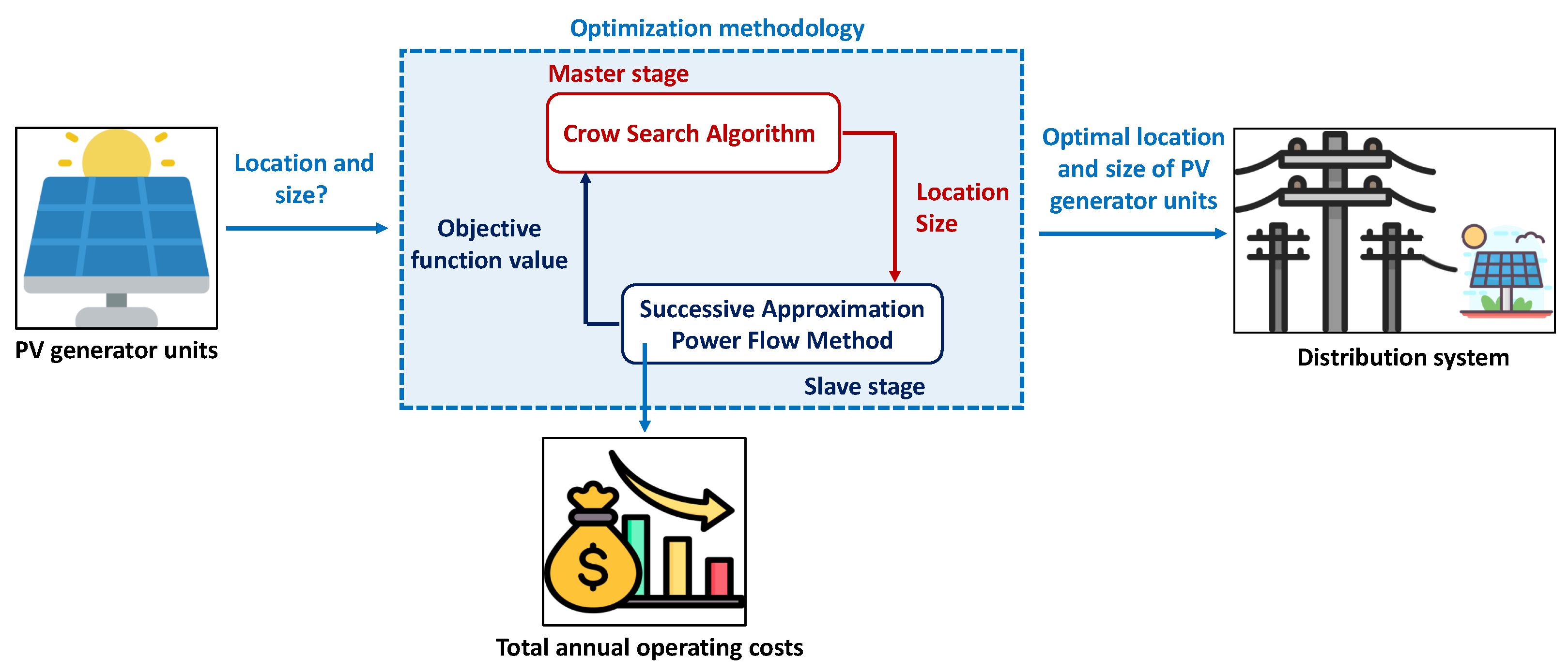
• A new master–slave methodology to solve the MINLP model that represents the problem under study. In this methodology, the master stage uses a Discrete–Continuous version of the Crow Search algorithm (DCCSA) to define the set of nodes where the PV generation units will be installed (location), as well as their corresponding nominal power (sizing). Meanwhile, the slave stage employs the successive approximation power flow method to evaluate the total annual operating costs of the network.
• A new master–slave methodology that finds a global optimal solution to the problem of optimally locating and sizing PV generation units in electrical systems and produces the best results in terms of solution quality and repeatability.

Figure 1 shows the graphical abstract that summarizes the contents of the article. The main idea of this research paper is to use a CSA-based master–slave methodology that employs the successive approximations power flow method for solving the problem of siting and sizing PV generation units to minimize the total annual operating costs in electrical distribution systems.

1.4. Structure of the Paper

This paper is organized as follows. Section 2 introduces the mathematical formulation of the problem regarding the optimal location and sizing of PV generation units in electrical systems, with the objective function being the reduction in the total annual operating costs. Section 3 presents the proposed methodology, which combines the DCCSA and the successive approximation power flow technique. Section 4 presents the main characteristics of the 33- and 69-node test systems, the generation and demand curves employed, and the parametric information necessary to find the value of the fitness function. Section 5 presents a discussion on the results obtained for the problem under analysis as well as the total annual operating costs. Finally, Section 6 outlines the conclusions and future lines of research.

2. Mathematical Formulation

The problem of optimally locating and sizing PV generation units in electrical systems can be expressed and solved using an MINLP model. In this model, the decision variables (i.e., those of a binary nature) are associated with the selection of the nodes where the PV generation units will be installed [18], whereas its nonlinearities appear in the formulation of the power flow due to the nonlinear nature of its equations [19,20].

The next subsections present the objective function and the set of constraints that represent the problem under analysis.

2.1. Formulation of the Objective Function

The main focus of power system planning projects is to recover the initial investment made by the grid operator. In this case study, in order to recover the investment made to integrate the PV generation units into electricity systems, the aim is the minimization of the total power purchase costs at the node that interconnects the distribution system with the transmission/subtransmission grid. Note that the installation and maintenance costs of the PV generation units are charged to the distribution system operators (DSO), as they are the body in charge of distributing and managing the power required to supply the demand of the users together with the system losses, in order to provide a service with high power quality that is as economical as possible.

In this context, the objective function considered is the reduction in the total annual operating costs of an electrical network, which will allow the initial investment to be recovered. Such costs include (i) the costs of purchasing energy at the main supply node (also known as the slack node or substation node), (ii) the investment in PV generation units, and (iii) their corresponding maintenance and operation costs. Such an objective function is presented in (1)–(4).

$$min{A}_{cost}=f_1+f_2+f_3,$$

(1)

$$f_1=C_{kWh}T{f}_a{f}_c\left(\sum _{h\in \mathcal{H}}\sum _{k\in \mathcal{N}}{p}_{k,h}^{cg}\mathsf{\Delta }h\right),$$

(2)

$$f_2=C_{pv}{f}_a\left(\sum _{k\in \mathcal{N}}{p}_k^{pv}\right),$$

(3)

$$f_3=C_{O\&M}T\left(\sum _{h\in \mathcal{H}}\sum _{k\in \mathcal{N}}{p}_{k,h}^{pv}\mathsf{\Delta }h\right),$$

(4)

with

$$\begin{array}{c}\hfill f_a=\left(\frac{t_a}{1-{(1+t_a)}^{-N_t}}\right),\end{array}$$

$$\begin{array}{c}\hfill f_c=\left(\sum _{t\in \mathcal{T}}{\left(\frac{1+t_e}{1+t_a}\right)}^t\right),\end{array}$$

where $A_{cost}$ is the objective function value and represents the total annual operating costs of the system. $f_1$ denotes the annual costs of purchasing energy at the main supply node. $f_2$ is the annual investment in PV generation units; and $f_3$ is their corresponding operation and maintenance costs. $C_{kWh}$ represents the average energy purchasing cost at the substation node. T is the number of days in an ordinary year (365). $f_a$ denotes the annuity factor that can be used to calculate the regular payments that the network operator must make, which are dependent on the expected internal return rate ($t_a$) and the planning horizon (years, $N_t$). $f_c$ represents the factor associated with the increase in the cost of energy during the planning period, which depends on the annual percentage rise in the cost of energy expected by the network operator ($t_e$). $p_{k,h}^{cg}$ is the active power produced by each conventional generator connected to node k in time period h. $\mathsf{\Delta }h$ denotes the time during which the electrical variables are assumed constant (i.e., 1 h for a one-day operation scenario). $C_{pv}$ represents the average installation cost for 1 kW of PV power. $p_k^{pv}$ is the nominal power of each PV generation unit connected to node k. $C_{O\&M}$ denotes the maintenance and operation costs associated with each PV generation unit. $p_{k,h}^{pv}$ represents the active power produced by each PV generation unit connected to node k in time period h. Finally, $\mathcal{N}$, $\mathcal{H}$, and $\mathcal{T}$ are the sets containing all the network nodes, the time periods in a one-day operation scenario, and the number of years in the planning horizon, respectively.

2.2. Set of Constraints

The set of constraints of the problem regarding the optimal placement and sizing of PV generation units in electrical systems represents the different operational limits found in such systems, such as active and reactive power balance, maximum and minimum capacities of each device, and voltage regulation bounds at each node in the system. Such constraints are presented in (5)–(13).

$$p_{k,h}^{cg}+p_{k,h}^{pv}-P_{k,h}^d=v_{k,h}\sum _{j\in \mathcal{N}}{Y}_{kj}{v}_{j,h}\cos \left({\theta }_{k,h}-{\theta }_{j,h}-{\phi }_{kj}\right),\left\{\begin{array}{cc}\forall k\in \mathcal{N},& \forall h\in \mathcal{H}\end{array}\right\},$$

(5)

$$q_{k,h}^{cg}-Q_{k,h}^d=v_{k,h}\sum _{j\in \mathcal{N}}{Y}_{kj}{v}_{j,h}\sin \left({\theta }_{k,h}-{\theta }_{j,h}-{\phi }_{kj}\right),\left\{\begin{array}{cc}\forall k\in \mathcal{N},& \forall h\in \mathcal{H}\end{array}\right\},$$

(6)

$$p_{k,h}^{pv}=p_k^{pv}{G}_h^{pv},\left\{\begin{array}{cc}\forall k\in \mathcal{N},& \forall h\in \mathcal{H}\end{array}\right\},$$

(7)

$$P_k^{cg,min}\le p_{k,h}^{cg}\le P_k^{cg,max},\left\{\begin{array}{cc}\forall k\in \mathcal{N},& \forall h\in \mathcal{H}\end{array}\right\},$$

(8)

$$Q_k^{cg,min}\le q_{k,h}^{cg}\le Q_k^{cg,max},\left\{\begin{array}{cc}\forall k\in \mathcal{N},& \forall h\in \mathcal{H}\end{array}\right\},$$

(9)

$$x_k{P}_k^{pv,min}\le p_k^{pv}\le x_k{P}_k^{pv,max},\left\{\begin{array}{c}\forall k\in \mathcal{N}\end{array}\right\},$$

(10)

$$v_k^{min}\le v_{k,h}\le v_k^{max},\left\{\begin{array}{cc}\forall k\in \mathcal{N},& \forall h\in \mathcal{H}\end{array}\right\},$$

(11)

$$\sum _{k\in \mathcal{N}}{x}_k\le N_{pv}^{avail},$$

(12)

$$x_k\in \left\{0,1\right\},\left\{\begin{array}{c}\forall k\in \mathcal{N}\end{array}\right\},$$

(13)

where $P_{k,h}^d$ and $Q_{k,h}^d$ are the active and reactive power demanded at node k in time period h, respectively. $q_{k,h}^{gc}$ denotes the reactive power produced by each conventional generator connected to node k in time period h. $v_{k,h}$ and $v_{j,h}$ denote the voltages at nodes k and j in time h, respectively. $Y_{kj}$ is the admittance relating nodes k and j and whose angle is ${\phi }_{k,j}$. ${\theta }_{k,h}$ and ${\theta }_{j,h}$ denote the voltage angles at nodes k and j in time period h, respectively. $G_h^{pv}$ represents the expected PV generation curve in the area of influence of the electrical system. $P_k^{cg,min}$ and $P_k^{cg,max}$ are the active power bounds for each conventional generator connected to the node k, whereas $Q_k^{cg,min}$ and $Q_k^{cg,max}$ denote the reactive power bounds for each conventional generator connected to node k. $P_k^{fv,min}$ and $P_k^{fv,max}$ represent the active power bounds for the PV generation units connected to node k. $x_k$ is the binary variable in charge of locating each PV generation unit in a node k of the system. $v_k^{min}$ and $v_k^{max}$ denote the minimum and maximum voltage regulation values allowed at each node that makes up the electrical system. Finally, $N_{fv}^{avail}$ represents a constant parameter related to the maximum number of PV generation units available for installation along the network.

2.3. Model Interpretation

The model presented in (1)–(13), which represents the problem of optimally locating and sizing PV generation units in electrical systems, can be interpreted as follows: Equation (1) defines the objective function of the problem, which is the sum of (i) the annual energy purchasing costs at the node that connects the electrical system with a transmission/distribution network, as shown in Equation (2); (ii) the annual investment in PV systems, as shown in Equation (3); and (iii) their corresponding maintenance and operation costs, as shown in Equation (4). Equality Equations (5) and (6) represent the active and reactive power balance at each system node in each time period, respectively. These are the most complex constraints in the problem under analysis, and, due to their nonlinear and nonconvex nature, they require numerical methods to be properly solved [21]. Equation (7) establishes that the active power produced by the PV generation units varies depending on their nominal power and the expected generation curve in the area of influence of the network. Inequality Equations (8) and (9) define the minimum and maximum active and reactive power injected by the conventional generators. Inequality Equation (10) determines the minimum and maximum active power produced by the PV generation units that will be installed along the system. Box-type Equation (11) presents the lower and upper voltage regulation bounds for all nodes and time periods. Equation (12) defines the maximum number of PV generation units available for installation along the network. Equation (13) shows the binary nature of the decision variable $x_k$.

Note that the MINLP model in Equations (1)–(13) is a general representation of the problem under study. The two main drawbacks of this model are (i) its nonlinearities and nonconvexities in the active and reactive power balance equations and (ii) the fact that it combines binary and integer variables. Consequently, as there might be multiple solutions to this model, which will be local optima, several authors have proposed using master–slave methods to solve it because they enable separating the continuous optimization problem from its discrete part [22].

Therefore, to solve the problem under study, this research presents a master–slave methodology that combines the DCCSA and the successive approximations method. This technique has not been reported in the specialized literature and belongs to the main contributions of this work.

3. Proposed Solution Methodology

To solve the problem of optimally locating and sizing PV generation units in electrical systems, which was described above, this study proposes using a master–slave methodology that employs a Discrete–Continuous version of the Crow Search Algorithm (DCCSA) [23] in the master stage and the successive approximations power flow method [24] (slave stage). In this methodology, the master stage defines the set of nodes where the PV generation units will be installed, as well as the size of such units, and the slave stage evaluates the objective function and constraints associated with network operation, which were presented in (5)–(13).

The next subsections present the codification used to represent the problem under analysis as well as each component of the proposed methodology (i.e., master stage and slave stage).

3.1. Proposed Codification

The DCCSA is the cornerstone of our proposed solution methodology because it is responsible for determining the optimal locations and sizes of PV generation units in electrical networks. To that end, each individual in the metaheuristic algorithm uses a discrete–continuous codification of the form

$$C_i^t=\left[\begin{array}{c}2,z,\dots ,n|0.0000,p_z^{pv},\dots ,2.4000\end{array}\right];i=1,2,...,N_i,$$

(14)

where $C_i^t$ is an individual i from population C at iteration t, whose size is $1\times \left(2N_{pv}^{avail}\right)$. z is a random number that defines the node where each PV generation unit will be installed. This number can take a value between 2 and the number of nodes in the system (i.e., n), which means that the PV generation units are only placed in the demand nodes. Finally, $N_i$ is the number of individuals in the population.

As can be seen in Equation (14), each individual in the population has two components: (i) the first $N_{pv}^{avail}$ parameters of the solution vector, which define the demand nodes where the PV generation units are to be installed, and (ii) the subsequent $N_{pv}^{avail}$ parameters of the solution vector, which determine the optimal sizes of each PV generation unit to be installed in the system.

The main advantage of this codification is that it allows the optimal location and sizing problem to be solved in a single stage by transforming the MINLP model defined from (1)–(13) into a nonlinear programming model. Consequently, the solution space can be efficiently explored and exploited in shorter processing times [16].

3.2. Master Stage: The Discrete–Continuous Version of the Crow Search Algorithm (DCCSA)

The DCCSA is a bio-inspired optimization metaheuristic algorithm, which is based on the intelligent behavior of crow flocks [23]. In the animal kingdom, crows are considered the smartest birds because they are capable of memorizing and remembering faces, using tools, communicating with one another, and properly feeding throughout the year [23]. They are known to be ambitious birds because they compete with one another for better food sources and pay attention to where other birds hide their food to steal it [25]. After stealing food, crows take the necessary precautions to avoid becoming victims, such as changing their hiding places and course [26].

This behavior can be modeled mathematically by considering the following simple principles in order to properly explore and exploit the solution space [23]:

✓

Crows live in flocks.

✓

Crows remember where they hide their food.

✓

Crows follow other crows to steal their food.

✓

Crows protect their hiding places from theft via stochastic processes.

3.2.1. Initial Population

The DCCSA is a population-based algorithm. The population in this algorithm consists of crows that are randomly located in the environment, which allows it to start exploring and exploiting the solution space. The structure of the initial population of crows is as shown below:

$$C^t=\left[\begin{array}{cccc}{C}_{11}^t& C_{12}^t& \cdots & C_{1N_v}^t\\ C_{21}^t& C_{22}^t& \cdots & C_{2N_v}^t\\ ⋮& ⋮& \ddots & ⋮\\ C_{N_{i}1}^t& C_{N_{i}2}^t& \cdots & C_{N_i,N_v}^t\end{array}\right],$$

(15)

where $C^t$ is the population of crows at iteration t, and $N_v$ is the number of variables or the dimension of the solution space, that is, the number of PV generation units to be installed in the electrical system and their sizes, i.e., $2N_{pv}^{ava}$.

To generate an initial population of crows that respects the structure shown in (14), Equation (16) is used. This equation creates a matrix of random numbers (within the lower and upper limits) containing all possible solutions.

$$C^0=y_{min}ones(N_i,N_v)+(y_{max}-y_{min})rand(N_i,N_v)$$

(16)

In (16), $ones(N_i,N_v)\in {\mathbb{R}}^{N_i\times N_v}$ is a matrix filled with ones. $rand(N_i,N_v)\in {\mathbb{R}}^{N_i\times N_v}$ is a matrix filled with random numbers between 0 and 1, which are generated with a uniform distribution. Finally, $y_{min}\in {\mathbb{R}}^{N_v\times 1}$ and $y_{max}\in {\mathbb{R}}^{N_v\times 1}$ are vectors that represent the lower and upper bounds of the solution space, respectively:

$$y_{min}=\left[\begin{array}{c}{y}_{1,min}\\ y_{2,min}\end{array}\right],y_{max}=\left[\begin{array}{c}{y}_{1,max}\\ y_{2,max}\end{array}\right],$$

where $y_{1,min}\in {\mathbb{R}}^{N_{pv}^{ava}\times 1}$ and $y_{1,max}\in {\mathbb{R}}^{N_{pv}^{ava}\times 1}$ denote the lower and upper bounds, respectively, of the decision variables related to the locations of the PV generation units in the demand nodes, and $y_{2,min}\in {\mathbb{R}}^{N_{pv}^{ava}\times 1}$ and $y_{2,max}\in \mathbb{R}{N}_{pv}^{ava}\times 1$ are the lower and upper bounds, respectively, of the decision variables associated with the sizes of the PV generation units.

Finally, at each iteration (t), each crow (i) in the population memorizes the position of its hiding place, as shown in Equation (17). This equation thus stores the position of the best food source found thus far by each crow. Note that crows memorize their best experience thanks to the fact that they move around in their environment in search of the best food source.

$$M^t=\left[\begin{array}{cccc}{C}_{11}^t& C_{12}^t& \cdots & C_{1N_v}^t\\ C_{21}^t& C_{22}^t& \cdots & C_{2N_v}^t\\ ⋮& ⋮& \ddots & ⋮\\ C_{N_{i}1}^t& C_{N_{i}2}^t& \cdots & C_{N_i,N_v}^t\end{array}\right]$$

(17)

3.2.2. Crows’ Movement

One could say that in iteration t, crow j wants to visit its hideout (i.e., best food source found thus far), which is at position $M_j^t$, and crow i decides to follow crow j to be near its cache. At this point, there are two possible scenarios:

1

Scenario 1: Search

In this scenario, crow j is unaware that crow i is following it. Hence, i can get close to the cache of crow j and updates its position in the solution space. This new position can be modeled mathematically as follows:

$$C_i^{t+1}=C_i^t+randfl(M_j^t-C_i^t),$$

(18)

where $rand$ is a random number between 0 and 1, generated with a uniform distribution, and $fl$ is the flight length of crow i. As per [23], small values of $fl$ allow for a local exploration of the solution space (close to $C_i^t$), whereas large values of $fl$ allow for a global exploration of the solution space (far from $C_i^t$).

2

Scenario 2: Evasion

In this scenario, crow j is aware that crow i is following it. Hence, to prevent its hidden food from being stolen, it tries to fool crow i by moving to a random position in the solution space.

These two scenarios can be summarized as follows:

$$C_i^{t+1}=\left\{\begin{array}{cc}{C}_i^t+randfl(M_j^t-C_i^t)& \mathrm{If}{r}_j\ge A_p\\ \mathrm{a}\mathrm{random}\mathrm{position}& \mathrm{otherwise}\end{array}\right.,$$

(19)

where $r_j$ is a random number between 0 and 1, which is generated by a uniform distribution, and $A_p$ is the probability that crow j finds out that crow i is following it.

3.2.3. Memory Updating

Once the position of the crows is updated considering the two scenarios described above, the new position of the food source must be memorized based on its quality. Thus, if the fitness function value of the new food source is better than the fitness function value of the previously memorized food source, crows update their memory with the new position:

$$M_i^{t+1}=\left\{\begin{array}{cc}{C}_i^{t+1}& \mathrm{If}{F}_F\left(C_i^{t+1}\right)<F\left(M_i^t\right)\\ M_i^t& \mathrm{otherwise}\end{array}\right.,$$

(20)

where $F_f(·)$ represents the fitness function to minimize.

3.2.4. General Implementation of the DCCSA

Algorithm 1 shows how the DCCSA is implemented to solve the problem addressed in this study.

Algorithm 1: Crow search algorithm used to solve optimization problems

1. Define parameters $N_i$, $Nv$, $A_p$, $fl$, $t_{max}$, $y^{min}$, and $y^{max}$

2. Generate the initial population using Equation (16)

3. Calculate the fitness function value (see Equation (24)) of each individual

4. Initialize the memory ($M_i^0$) of each crow (i)

5. for$t\le t_{max}$do

14. Result: The best solution is found for $C_i^{t_{max}}$, and its fitness function is $F\left(C_i^{t_{max}}\right)$.

3.3. Slave Stage: Successive Approximation Power Flow Method

The successive approximation method used to solve the power flow in electrical systems was first introduced by Montoya and Gil-González in [24]. The active and reactive power balance equations given by (5) and (6), respectively, can be solved iteratively using this method. It enables the slave stage to evaluate the fitness function value for each individual in the population of crows while ensuring that the constraints specified in the MINLP model (described in Section 2) are respected. Likewise, this method was selected because it requires short processing times and rapidly converges toward the solution.

The recursive formula that can be employed to solve the power flow presented in (5) and (6) is given by

$${\mathbb{V}}_{d,h}^{t+1}=-{\mathbf{Y}}_{dd}^{-1}\left[{\mathbf{diag}}^{-1}\left({\mathbb{V}}_{d,h}^{t,*}\right)({\mathbb{S}}_{d,h}^{*}-{\mathbb{S}}_{pv,h}^{*})+{\mathbf{Y}}_{ds}{\mathbb{V}}_{s,h}\right],$$

(21)

where t is the iteration counter. ${\mathbb{V}}_{d,h}$ denotes the vector that contains the voltage at the demand nodes for each time period h, i.e., the variables of interest. ${\mathbf{Y}}_{ds}$ is the component of the admittance matrix that associates the slack node with the demand nodes, whereas ${\mathbf{Y}}_{dd}$ denotes the component of the admittance matrix that relates the demand nodes to each other. ${\mathbb{S}}_{d,h}$ represents the vector in the complex domain that contains the active and reactive power demanded at the load nodes for each time period h. ${\mathbb{S}}_{pv,h}$ is the vector in the complex domain that contains the active power produced by each PV unit for each time period h. ${\mathbb{V}}_{s,h}$ denotes the vector that contains the voltage at the terminals of the substation node for each time period h, which is a known parameter in the solution of the power flow. Finally, $\mathbf{diag}\left(z\right)$ represents a diagonal matrix made up of the elements of vector z.

To assess the convergence of the iterative process, the criterion shown in (22) is used. According to this criterion, the maximum difference between the demand voltages (i.e., ${\mathbb{V}}_{d,h}$) for each time period h in two consecutive iterations should be below a predefined threshold.

$$\underset{h}{max}\left\{\begin{array}{c}\left|\right|{\mathbb{V}}_{d,h}^{t+1}|-|{\mathbb{V}}_{d,h}^t\left|\right|\end{array}\right\}\le \zeta$$

(22)

In (22), $\zeta$ represents the convergence error, which, for the purposes of this study, will be $1\times {10}^{-10}$, as recommended by the authors of [24].

Once the power flow is solved for all time periods h using the successive approximation method, the power produced at the terminals of the substation node must then be calculated, as follows:

$${\mathbb{S}}_{s,h}^{*}=\mathbf{diag}\left({\mathbb{V}}_{s,h}^{*}\right)\left({\mathbf{Y}}_{ss}{\mathbb{V}}_{s,h}+{\mathbf{Y}}_{sd}{\mathbb{V}}_{d,h}\right),$$

(23)

where ${\mathbb{S}}_{s,h}$ denotes the vector in the complex domain that contains the active and reactive power produced at the slack node for each time period h. ${\mathbf{Y}}_{ss}$ is the component of the admittance matrix associated with the slack node, while ${\mathbf{Y}}_{sd}$ is the component of the admittance matrix that associates the slack node to the demand ones.

Note that the value of $f_1$ can be obtained by solving (23). Similarly, the solutions provided by each individual in the master stage, which respect the codification established in (14), can be used to obtain the value of $f_2$ and $f_3$. However, to rule out possible infeasible solutions, which violate the boundaries of the solution space, the objective function described in (1) is replaced by the fitness function shown in (24) [27,28].

$$\begin{array}{cc}\hfill F_f=& A_{cost}+{\beta }_1\underset{h}{max}\left\{0,|{\mathbb{V}}_{d,h}|-v^{max}\right\}-{\beta }_2\underset{h}{min}\left\{0,|{\mathbb{V}}_{d,h}|-v^{min}\right\}\hfill \\ \hfill & -{\beta }_3\underset{h}{min}\left\{0,\mathrm{real}({\mathbb{S}}_{s,h}-P_k^{gc,min})\right\}\hfill \end{array}$$

(24)

In (24), $F_f$ is the value of the fitness function, and ${\beta }_1$, ${\beta }_2$, and ${\beta }_3$ denote the penalty factors applied to the objective function. These penalty factors come into play when the solutions provided by the master stage violate the voltage regulation constraints or power generation capacities at the substation node. In this study, the value of such penalty factors is $1\times {10}^6$, and each penalty factor has its corresponding unit.

One of the main advantages of using a fitness function is that it helps the metaheuristic optimization algorithm to efficiently explore and exploit the solution space. If all the constraints presented in (5)–(13) are met, the final value of $F_f$ equals the original value of the objective function ($A_{cost}$). If not, the solution is discarded as a possible optimal solution [29].

4. Test Systems

To validate the master–slave methodology proposed in this paper to solve the problem of optimally locating and sizing PV generation units in electrical systems, the 33- and 69-node test systems were used, both of which have a radial topology [30]. These test systems are selected for the sake of comparison, as they have been previously used in the literature to solve the problem of locating and sizing PV generation units. This allows evaluating and comparing the best response, repeatability, and processing times of the proposed master–slave methodology. The next subsections present the main characteristics of each test system.

4.1. First Test Feeder: 33-Node Test System

This system consists of 33 nodes and 32 distribution lines, as shown in Figure 2. It operates at a base voltage of 12.66 kV and a base power of 100 kVA. In the peak power consumption scenario, the loads of this system demand $\left(3715+j2300\right)$ kVA. Its parametric information can be found in [31].

4.2. Second Test Feeder: 69-Node Test System

This system consists of 69 nodes and 68 distribution lines, as illustrated in Figure 2. It operates at a base voltage of 12.66 kV and a base power of 100 kVA. In the peak power consumption scenario, the loads of this system demand $\left(3890.7+j2693.6\right)$ kVA. Its parametric information can be found in [31].

4.3. Calculation of the Objective Function

To calculate the value of the fitness function defined in (24), the parametric data shown in

Table 1. Parameters used to calculate the objective function.

Parameter	Value	Unit	Parameter	Value	Unit
$C_{kWh}$	0.1390	USD/kWh	T	365	days
$t_a$	10	%	$N_t$	20	years
$\mathsf{\Delta }h$	1	h	$t_e$	2	%
$C_{pv}$	1036.49	USD/kWp	$C_{0\&M}$	0.0019	USD/kWh
$N_{pv}^{avail}$	3	-	$\mathsf{\Delta }V$	$\pm 10$	%
$P_k^{pv,min}$	0	kW	$P_k^{pv,max}$	2400	kW
${\beta }_1$	$1\times {10}^6$	USD/V	${\beta }_2$	$1\times {10}^6$	USD/V
${\beta }_3$	$1\times {10}^6$	USD/W	-	-	-

were used [32,33].

To assess the impact of integrating PV generation units in the systems described above, typical generation and demand curves reported for Medellín (Colombia) were used, which are illustrated in Figure 3.

5. Numerical Results and Discussion

This section discusses the numerical results obtained by the DCCSA in solving the problem of optimally locating and sizing PV generation units in the two test systems under analysis. To show the efficiency of the proposed metaheuristic algorithm, it was compared against the following six methods, which have also been used to solve the same problem: (i) the BONMIN solver of the GAMS (exact solution to the MINLP model) [14], (ii) the Discrete–Continuous version of the Chu and Beasley Genetic Algorithm (DCCBGA) [14], (iii) the Discrete–Continuous version of the Newton Metaheuristic Algorithm (DCNMA) [15], (iv) the Discrete–Continuous version of the Vortex Search Algorithm (DCVSA) [12], (v) the Discrete–Continuous version of the Generalized Normal Distribution Optimizer (DCGNDO) [16], and (vi) the Discrete–Continuous version of the Parallel Particle Swarm Optimization (DCPPSO) algorithm [17].

For both test systems, this study considered installing three PV generation units, each with a maximum capacity of 2400 kW. All simulations were performed in MATLAB (version $2022a$) using our own scripts on a desktop computer with an Intel(R) Core(TM) i9-11900 CPU@2.50Ghz processor and 64.0 GB RAM, which was running 64-bit Windows 10 Pro.

5.1. DCCSA Parameters

The information presented in

Table 2. Parameters of the DCCSA employed in the master stage.

Parameter	DCCSA
Number of individuals ($N_i$)	87
Maximum iterations ($t_{max}$)	816
Flight length ($fl$)	2.8741
Awareness probability ($A_p$)	0.0046

was used to implement the master–slave methodology proposed in this study to solve the problem of optimally locating and sizing PV generation units in electrical systems.

To define the parameters shown in Table 2, the DCCSA was tuned using the Chu and Beasley genetic algorithm [34], with an initial population of 50 individuals and a maximum number of iterations of 350 for the 69-node test system because it is the largest of the two systems used to validate the proposed methodology. The tuning parameters were: (i) a population size ($N_i$) in the [1, 100] range, (ii) a maximum number of iterations ($t_{max}$) in the [1, 1000] range, (iii) a flight length ($fl$) in the [0, 3.5] range, and (iv) an awareness probability ($A_p$) in the [0, 1] range. Moreover, the proposed methodology was evaluated 100 consecutive times to find the best, average, and worst values for the objective function. Additionally, the standard deviation and average time required by the algorithm to determine the optimal locations and sizes of the PV generation units were calculated for the two test systems under analysis.

5.2. Results Obtained in the First Test System under Analysis

5.2.1. Numerical Results

Table 3. Numerical results obtained in the 33-node test system.

Method	Location (Node)/Power (MW)	${\mathit{A}}_{\mathit{cost}}$ (USD/Year)	Reduction (%)	Time (s)	STD (%)
Base case	-	3,700,455.38	0	-	-
	-
	-
BONMIN	17/1.3539	2,701,824.14	26.9867	3.64	0
	18/0.2105
	33/2.1452
DCNMA	8/2.0961	2,700,227.33	27.0298	20.21	0.0812
	16/1.2688
	30/0.2770
DCCBGA	11/0.7605	2,699,932.29	27.0378	5.30	0.0452
	15/0.9690
	30/1.9060
DCVSA	11/0.7606	2,699,761.71	27.0424	170.23	0.0427
	14/1.0852
	31/1.8030
DCGNDO	10/1.0083	2,699,671.76	27.0436	268.69	0.0700
	16/0.9137
	31/1.7257
DCPPSO	10/1.0092	2,699,671.76	27.0436	8.32	0.0246
	16/0.9137
	31/1.7245
DCCSA	10/1.0093	2,699,671.76	27.0449	77.00	0.0037
	16/0.9138
	31/1.7246

shows the numerical results of the proposed methods and of those used as comparison in the 33-node test system. From left to right, this table specifies the methodology implemented, the nodes where the PV generation units were installed and their nominal power, the annual operating costs provided by each solution methodology, the reduction percentage obtained by each methodology with respect to the base case (values reported in the second row), the average processing time, and the standard deviation.

According to the information in Table 3, the solution provided by each metaheuristic algorithm outperformed that by the BONMIN solver (i.e., the exact solution to the MINLP model), which confirms that the presence of binary variables causes conventional optimization techniques to get stuck in local optima. Additionally, the proposed DCCSA, like the DCGNDO and the DCPPSO, managed to reduce the total annual operating costs by 1,000,783.62 USD/year when compared to the base case. This suggests that the global optimal solution for this test system is 2,699,671.76 USD/year, which is found by placing the PV generation units at nodes 10, 16, and 31, for a total installed capacity of 3647.65 kWp. Finally, all the methods allowed a reduction of more than 26.95% with respect to the base case, with the DCCSA allowing the highest reduction (27.0449%). When compared to the other methods in terms of reduction in total annual operating costs, the DCCSA outperformed the BONMIN solver by 0.0581%, the DCNMA by 0.0151%, the DCCBGA by 0.0071%, the DCVSA by 0.0025%, and the DCGNDO and the DCPPSO by 0.0013%.

5.2.2. Statistical Analysis

To show the effectiveness and robustness of the DCCSA in solving the problem of optimally locating and sizing PV generation units in electrical systems, it was run 100 consecutive times in the 33-node test system. The results of such validation are illustrated in Figure 4, which shows the improvements obtained by the DCCSA in terms of best solution, processing time, and standard deviation when compared to the other solution methodologies. The numbers in red indicate that the method used for comparison outperformed the DCCSA.

As observed in Figure 4, the DCCSA produced the best results in terms of reduction in annual operating costs when compared to the other methods. It outperformed the BONMIN solver by 0.0797%, the DCNMA by 0.0206%, the DCCBGA by 0.0097%, the DCVSA by 0.0053%, and the DCNGDO and the DCPPSO by $1\times {10}^{-7}$%.

Regarding processing times, the BONMIN solver, the DCNMA, the DCCBGA, and the DCPPSO were faster than the proposed solution methodology. When compared to the DCCSA, they reduced processing times by 95.2727%, 73.7529%, 93.1168%, and 89.1947%, respectively. Importantly, these differences in processing times are attributed to the fact that the population size employed for the proposed DCCSA included 77 more individuals than those used for the other methods. This means that at each iteration, the proposed algorithm had to evaluate 1848 power flows more than the other techniques. The DCCSA, however, was faster than the DCVSA and the DCNGDO; it reduced processing times by 121.0809% and 248.6963% when compared to the DCVSA and the DCNGDO, respectively. The processing times obtained by the DCCSA can be considered negligible when compared to the planning horizon chosen for this study (i.e., 20 years).

As for the standard deviation, the proposed DCCSA was superior to the other methods, as it achieved an improvement of 2075.4620% with respect to the DCNMA, of 1109.8241% with respect to the DCCBGA, of 1043.0023% with respect to the DCVSA, of 1775.1372% with respect to the DCNGDO, and of 559.0663% with respect to the DCPPSO. Note that in this case, the DCCSA was not compared to the BONMIN solver. The reason for this is that the solution of the BONMIN solver will always be the same because it is an exact solution to the MINLP model, so even if it is run 100 times, its standard deviation will always be 0.

The results mentioned above confirm the effectiveness and reliability of the DCCSA, as when solving the problem of optimally locating and sizing PV generation units in electrical networks to reduce the annual operating costs, it produced the best results in terms of solution quality and repeatability. Hence, the proposed methodology is regarded as the best option to solve such a problem in the 33-node test system.

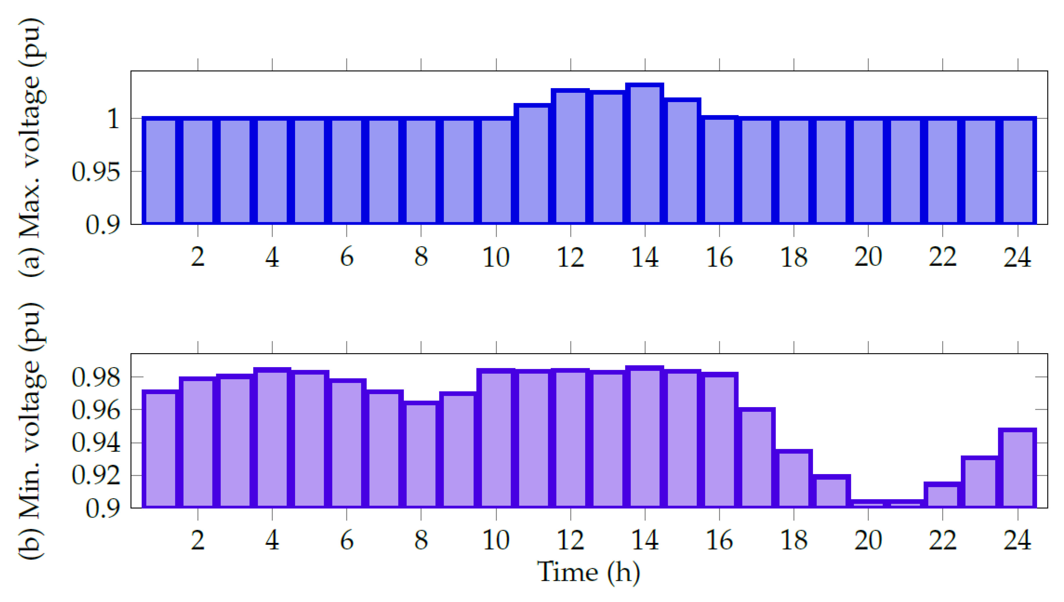
5.2.3. Feasibility Check

To verify that the optimal solution yielded by the DCCSA is feasible, i.e., it satisfies the electrical constraints proposed by the mathematical model presented in (5)–(13) and considered in the formulation of the fitness function given by (24), the active power generation at the main supply node was analyzed before and after implementing the solution obtained by the proposed methodology (see Figure 5).

When the solution provided by the DCCSA was implemented in the 33-node test system, the power produced by the slack node was inversely proportional to the power produced by the PV units. This means that as the power produced by the PV units increased from hour 7 to 14 (see Figure 3), the power produced at the substation node decreased until it hit zero (right when the PV power reached its maximum value). Similarly, as the power produced by the PV units decreased from hour 15 to 20, the power produced at the slack node increased. This proves that power generation respected the capacity constraint, as it yielded positive or zero values.

Finally, to confirm that the voltage profiles were within the regulation bounds (i.e., $\pm 10\%$), the behavior of the minimum and maximum voltages was examined for all time periods once the solution provided by the DCCSA was implemented (see Figure 6).

As may be concluded from Figure 6, the minimum and maximum voltage values in all time periods respected the voltage regulation bounds, as they remained within $\pm 10\%$. Additionally, the maximum voltage (i.e., 1.0322 pu) was recorded at node 16 when the PV units injected 100% of their nominal power. The minimum voltage (i.e., 0.9038 pu), which coincided with the minimum voltage of the base case, was recorded at node 18 when the PV units did not inject power and during the period of peak demand (from hour 20 to hour 21).

5.3. Results Obtained in the Second Test System under Analysis

5.3.1. Numerical Results

Table 4. Numerical results obtained in the 69-node test system.

Method	Location (Node)/Power (MW)	${\mathit{A}}_{\mathit{cost}}$ (USD/Year)	Reduction (%)	Time (s)	STD (%)
Base case	-	3,878,199.93	0	-	-
	-
	-
DCNMA	12/0.0794	2,826,368.60	27.1216	91.81	0.1900
	60/1.3805
	61/2.3776
DCCBGA	24/0.5326	2,825,783.33	27.1397	22.36	0.0999
	61/1.8954
	64/1.3772
DCVSA	16/0.2632	2,825,264.56	27.1502	887.64	0.0942
	61/2.2719
	63/2.2934
DCGNDO	21/0.4812	2,824,923.38	27.1589	1237.23	0.2558
	61/2.4
	64/0.9259
DCPPSO	21/0.4890	2,824,923.29	27.1589	55.15	0.0267
	61/2.4
	64/0.9169
DCCSA	21/0.4816	2,824,923.05	27.1589	377.49	0.0225
	61/2.4
	64/0.9254

, which was organized the same way as Table 3, shows the numerical results of the proposed technique and the methods used for the sake of comparison in the 69-node test system. Importantly, the BONMIN solver was not employed for comparison purposes in this test system because it failed to converge to any feasible solution. This can be explained by the fact that the solution space in this test system was larger than that in the first test system.

According to the information in Table 4, the proposed DCCSA provided the best solution for the 69-node test system, with a reduction in the total annual operating costs of approximately 1,053,276.87 USD/year with respect to the base case. This means that the optimal solution for this test system is 2,824,923.05 USD/year, which is found by placing the PV generation units at nodes 21, 61, and 64, for a total installed capacity of 3807.02 kWp. Moreover, all the methods used to solve the problem addressed in this paper allowed a reduction of more than 27% with respect to the base case, with the DCGNDO, the DCPPSO, and the DCCSA allowing the highest reduction (27.1589%). When compared to the other methods in terms of reduction in the annual operating costs, the proposed methodology outperformed the DCNMA by 0.0373%, the DCCBGA by 0.0192%, and the DCVSA by 0.0087%.

5.3.2. Statistical Analysis

As in the previous test system, the proposed methodology was run 100 consecutive times in the 69-node test system to validate its efficiency and robustness in solving the problem of optimally locating and sizing PV generation units in electrical systems. The results of such validation are shown in Figure 7, which shows the improvements obtained by the DCCSA in terms of best solution, processing time, and standard deviation when compared to the other solution methodologies. The numbers in red indicate that the method used for comparison outperformed the DCCSA.

As can be seen in Figure 7, the DCSSA provided the best results in terms of reduction in annual operating costs when compared to the others methods. It outperformed the DCNMA by 0.0512%, the DCCBGA by 0.0306%, the DCVSA by 0.01198%, the DCGNDO by $1.1589\times {10}^{-5}$%, and the DCPPSO by $8.621\times {10}^{-6}$%.

Regarding processing times, the DCNMA, the DCCBGA, and the DCPPSO were faster than the proposed methodology. When compared to the DCCSA, they reduced processing times by 75.6789%, 94.0767%, and 85.3903%, respectively. Importantly, these differences in processing time are attributed to the population size used for the DCCSA. The DCCSA, however, was faster than the DCVSA and the DCGNDO; it reduced processing times by 135.1417% and 227.75044% when compared to the DCVSA and the DCGNDO, respectively. The processing times obtained by the DCCSA can be considered negligible when compared to the planning horizon chosen for this study (i.e., 20 years).

As for the standard deviation, the proposed DCCSA produced the best results, as it achieved an improvement of 743.5249% with respect to the DCNMA, of 343.5967% with respect to the DCCBGA, of 318.4626% with respect to the DCVSA, of 1035.6953% with respect to the DCNGDO, and of 18.6085% with respect to the DCPPSO.

According to this, the proposed DCCSA provided the best results in terms of solution quality and repeatability, which makes it the best option for solving the problem of optimally locating and sizing PV generation units in the 69-node test system.

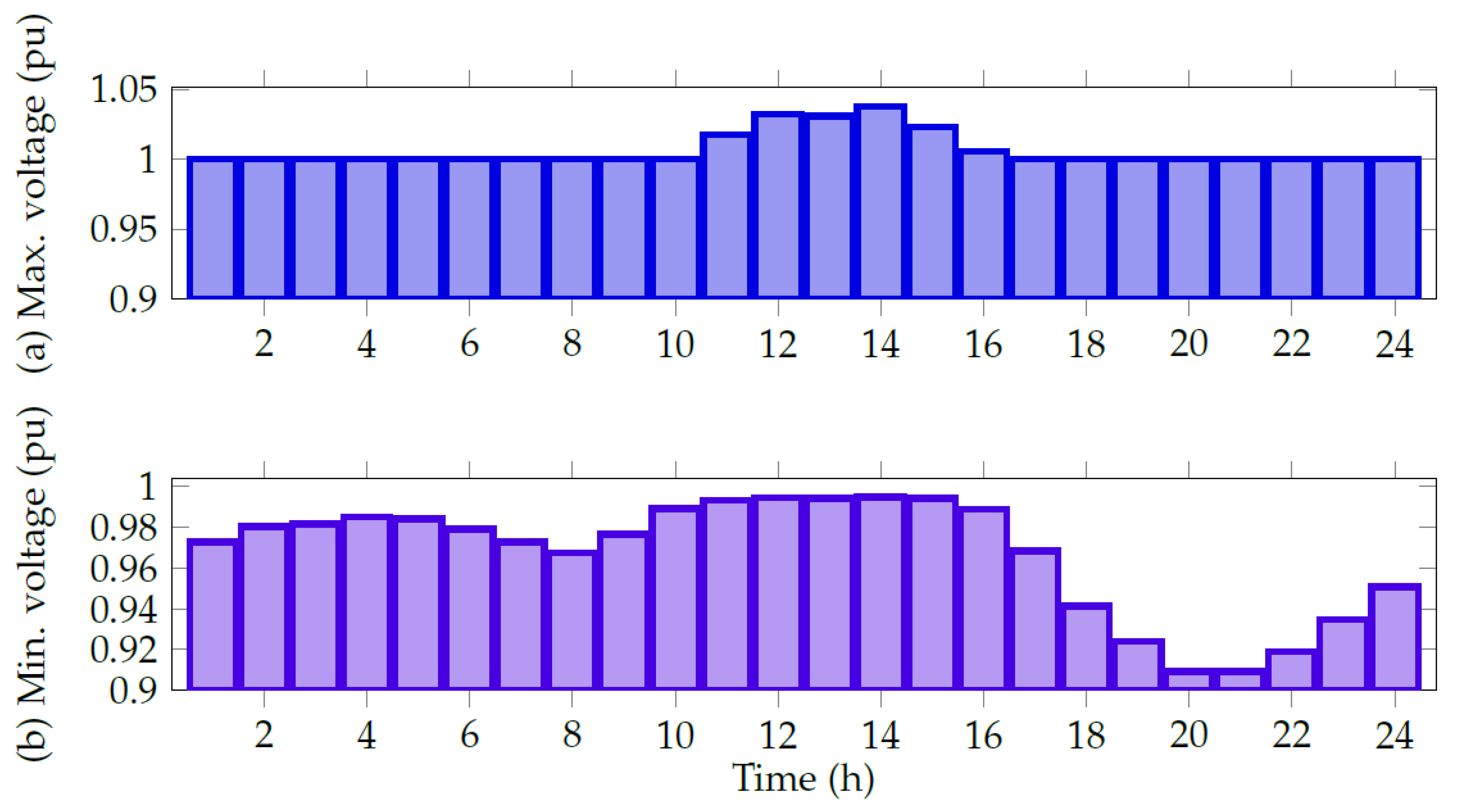
5.3.3. Feasibility Check

To verify whether the optimal solution yielded by the DCCSA is feasible, the active power generation at the main supply node was evaluated before and after implementing the solution obtained by the proposed methodology (see Figure 8).

Before implementing the solution provided by the DCCSA, the power produced at the slack node followed the same behavior of the demanded active power (see Figure 3) along with the system losses. However, once the best solution delivered by the DCCSA was implemented, the power produced at the slack node significantly decreased as the power produced by the PV units increased until it hit zero in time period 14 when the PV units injected 100% of their capacity. This proves that power generation at the slack node respected the capacity constraint, as it yielded positive or zero values.

Finally, to confirm that the voltage profiles were within the regulation bounds (i.e., $\pm 10\%$), the behavior of the minimum and maximum voltages was examined for all time periods once the solution delivered by the DCCSA was implemented (see Figure 9).

As may be concluded from Figure 9, the minimum and maximum voltage values in all time periods respected the voltage regulation bounds, as they remained within $\pm 10\%$. In addition, the maximum voltage (i.e., 1.0322 pu) was recorded at node 64 when the PV units injected 100% of their nominal power. The minimum voltage (i.e., 0.9092 pu), which coincided with the minimum voltage of the base case, was recorded at node 65 when the PV units did not inject power and during the period of peak demand (from hour 20 to 21).

6. Conclusions and Future Work

This study presented a master–slave method that employs a discrete–continuous version of the Crow Search Algorithm to solve the problem of optimally locating and sizing PV generation units in electrical networks. In the slave stage, the DCCSA is responsible for defining the set of nodes where the PV generation units are to be installed as well as the sizes of such units. In the slave stage, the successive approximations power flow method is in charge of finding the fitness function value. The objective function was the reduction in the total annual operating costs of a electrical network, which include (i) the energy purchasing costs at the main supply node, (ii) the investment in the PV generation units, and (iii) their corresponding operation and maintenance costs. The parameters of the proposed methodology were tuned using the CBGA.

The numerical results generated by our solution method in the 33- and 69-node test systems proved its applicability and effectiveness in comparison with other six methods reported in the specialized literature (the BONMIN solver of the GAMS, the DCCBGA, the DCNMA, the DCVSA, the DCGNDO, and the DCPPSO algorithm). The following are the key findings of this study:

✓

The DCCSA managed to reduce the total annual operating costs by approximately 1,000,783.62 USD/year and 1,053,276.87 USD/year in the 33- and 69-node test systems, respectively. These values represent reductions of 27.0449% and 27.1589%. These are the largest reductions found for the problem of locating and sizing PV generation units, which indicates that the overall optimal solutions to this problem for both test systems are 2,699,671.76 USD/year and 2,824,923.05 USD/year, respectively.

✓

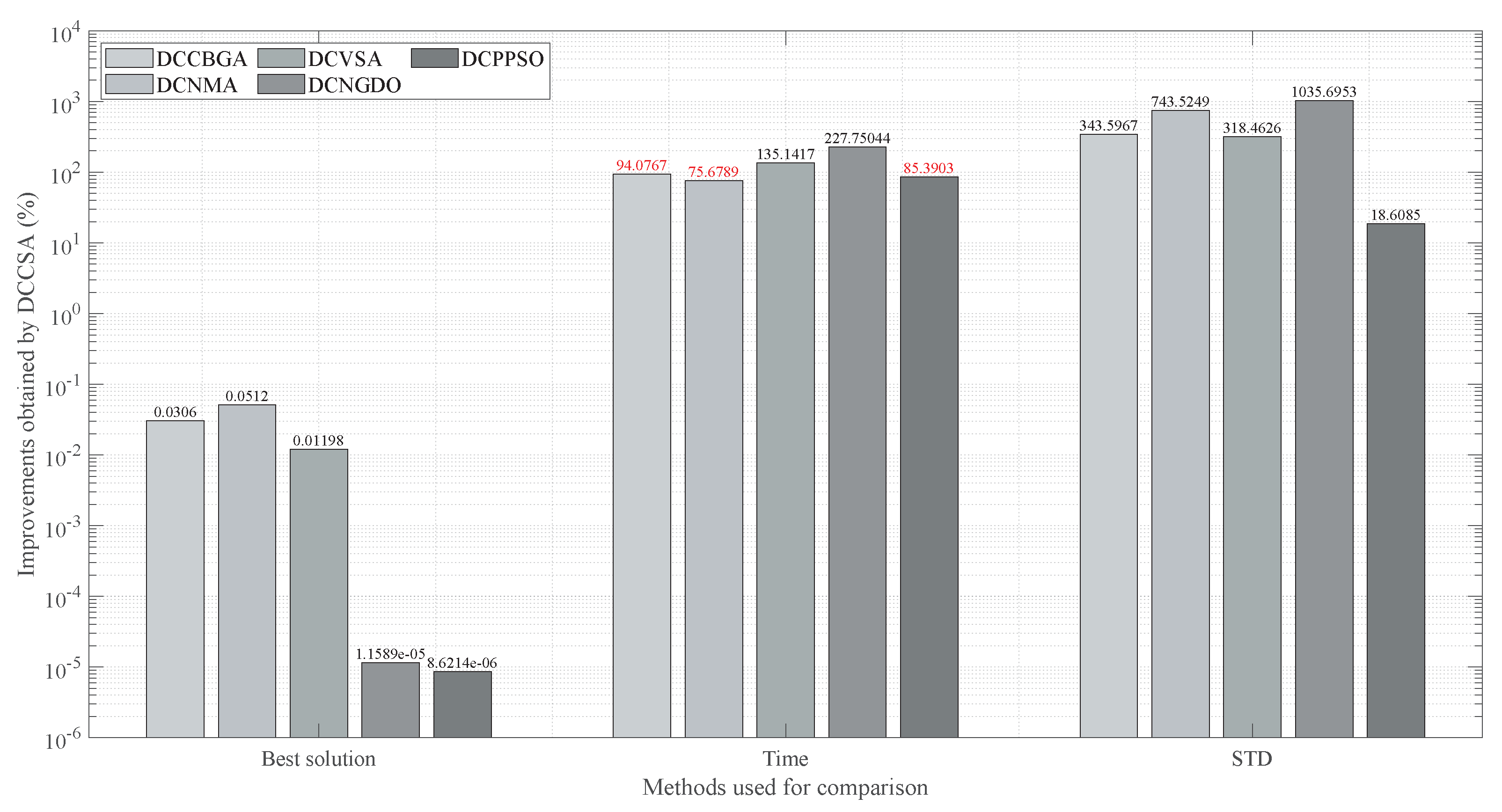
After 100 consecutive evaluations, the proposed DCCSA showed the lowest standard deviation values in both test systems, with improvements of 559.0663% and 18.6085% with respect to the DCPPSO (the second method with the best results) in the 33- and 69-node test systems, respectively. These results confirm the repeatability and robustness of the DCCSA in solving the problem under study, which makes the methodology used in this study the best option (i.e., over the other methodologies used in this topic) to solve the problem regarding the location and sizing of PV generation units. Moreover, this guarantees that in each evaluation, the solutions will be close to 80 USD/year and 637 USD/year for the 33- and 69-node test systems, respectively.

✓

The processing times required by the proposed technique to find an optimal and feasible solution was 76.9990 s in the 33-node test system and 377.4915 s in the 69-node test system. These are good values, considering that at each iteration, the DCCSA evaluated 1848 power flows more than the other methods. Additionally, processing times are not critical in power system planning because the quality of the solution provided by the methodology is what really matters.

✓

Due to the nonlinearities and nonconvexities of the mathematical model used to express the problem of optimally locating and sizing PV generation units in electrical systems, the complexity of the problem rises as the number of nodes increases. As a result, the BONMIN solver of the GAMS was unable to find an optimal solution in the 69-node test system. The proposed DCCSA, on the contrary, was found to be independent of the number of nodes in the electrical system because it produced the best results in terms of reductions in the total annual operating costs and standard deviation, even as the complexity of the problem increased. This allows concluding that the proposed DCCSA is the best option to solve the problem under analysis. Yet, as the number of system nodes increases, so does the size of the solution space, which implies that the time required to find an optimal solution will increase as well.

Based on our findings, future studies could reformulate the mathematical model of the problem under study, taking into account the maximum thermal current supported by the conductors in an electrical network. They could also solve the problem addressed in this paper using a multi-objective optimization approach that improves not only economic but also technical and environmental aspects that represent the operating conditions of electrical systems. Finally, the optimal conductor selection problem could be included in power system planning, and the costs associated with the investment in each conductor could be considered.

References

1. Saeed, M.H.; Fangzong, W.; Kalwar, B.A.; Iqbal, S. A Review on Microgrids’ Challenges & Perspectives. IEEE Access 2021, 9, 166502–166517. [Google Scholar]
2. Pimm, A.J.; Palczewski, J.; Barbour, E.R.; Cockerill, T.T. Using electricity storage to reduce greenhouse gas emissions. Appl. Energy 2021, 282, 116199. [Google Scholar] [CrossRef]
3. González, D.M.L.; Rendon, J.G. Opportunities and challenges of mainstreaming distributed energy resources towards the transition to more efficient and resilient energy markets. Renew. Sustain. Energy Rev. 2022, 157, 112018. [Google Scholar] [CrossRef]
4. Valencia, A.; Hincapie, R.A.; Gallego, R.A. Optimal location, selection, and operation of battery energy storage systems and renewable distributed generation in medium–low voltage distribution networks. J. Energy Storage 2021, 34, 102158. [Google Scholar] [CrossRef]
5. IPSE. Boletín Datos IPSE Mayo 2022; IPSE: Bogotá, Colombia, 2021. [Google Scholar]
6. López, A.R.; Krumm, A.; Schattenhofer, L.; Burandt, T.; Montoya, F.C.; Oberländer, N.; Oei, P.Y. Solar PV generation in Colombia-A qualitative and quantitative approach to analyze the potential of solar energy market. Renew. Energy 2020, 148, 1266–1279. [Google Scholar] [CrossRef]
7. Eltawil, M.A.; Zhao, Z. Grid-connected photovoltaic power systems: Technical and potential problems—A review. Renew. Sustain. Energy Rev. 2010, 14, 112–129. [Google Scholar] [CrossRef]
8. Cabrera, J.B.; Veiga, M.F.; Morales, D.X.; Medina, R. Reducing power losses in smart grids with cooperative game theory. In Advanced Communication and Control Methods for Future Smartgrids; Intechopen: London, UK, 2019; p. 49. [Google Scholar]
9. Almadhor, A.; Rauf, H.T.; Khan, M.A.; Kadry, S.; Nam, Y. A hybrid algorithm (BAPSO) for capacity configuration optimization in a distributed solar PV based microgrid. Energy Rep. 2021, 7, 7906–7912. [Google Scholar] [CrossRef]
10. Ngamprasert, P.; Rugthaicharoencheep, N.; Woothipatanapan, S. Application Improvement of Voltage Profile by Photovoltaic Farm on Distribution System. In Proceedings of the 2019 IEEE International Conference on Power, Energy and Innovations (ICPEI), Pattaya, Thailand, 16–18 October 2019; pp. 98–101. [Google Scholar]
11. Al Abri, R.; El-Saadany, E.F.; Atwa, Y.M. Optimal placement and sizing method to improve the voltage stability margin in a distribution system using distributed generation. IEEE Trans. Power Syst. 2012, 28, 326–334. [Google Scholar] [CrossRef]
12. Cortés-Caicedo, B.; Molina-Martin, F.; Grisales-Noreña, L.F.; Montoya, O.D.; Hernández, J.C. Optimal Design of PV Systems in Electrical Distribution Networks by Minimizing the Annual Equivalent Operative Costs through the Discrete-Continuous Vortex Search Algorithm. Sensors 2022, 22, 851. [Google Scholar] [CrossRef] [PubMed]
13. Jiang, S.; Wan, C.; Chen, C.; Cao, E.; Song, Y. Distributed photovoltaic generation in the electricity market: Status, mode and strategy. CSEE J. Power Energy Syst. 2018, 4, 263–272. [Google Scholar] [CrossRef]
14. Montoya, O.D.; Grisales-Noreña, L.F.; Perea-Moreno, A.J. Optimal Investments in PV Sources for Grid-Connected Distribution Networks: An Application of the Discrete–Continuous Genetic Algorithm. Sustainability 2021, 13, 13633. [Google Scholar] [CrossRef]
15. Montoya, O.D.; Grisales-Noreña, L.F.; Alvarado-Barrios, L.; Arias-Londoño, A.; Álvarez-Arroyo, C. Efficient reduction in the annual investment costs in AC distribution networks via optimal integration of solar PV sources using the newton metaheuristic algorithm. Appl. Sci. 2021, 11, 11525. [Google Scholar] [CrossRef]
16. Montoya, O.D.; Grisales-Noreña, L.F.; Ramos-Paja, C.A. Optimal Allocation and Sizing of PV Generation Units in Distribution Networks via the Generalized Normal Distribution Optimization Approach. Computers 2022, 11, 53. [Google Scholar] [CrossRef]
17. Grisales-Noreña, L.F.; Montoya, O.D.; Hernández, J.C.; Ramos-Paja, C.A.; Perea-Moreno, A.J. A Discrete-Continuous PSO for the Optimal Integration of D-STATCOMs into Electrical Distribution Systems by Considering Annual Power Loss and Investment Costs. Mathematics 2022, 10, 2453. [Google Scholar] [CrossRef]
18. Duong, M.Q.; Pham, T.D.; Nguyen, T.T.; Doan, A.T.; Tran, H.V. Determination of optimal location and sizing of solar photovoltaic distribution generation units in radial distribution systems. Energies 2019, 12, 174. [Google Scholar] [CrossRef] [Green Version]
19. Khoso, A.H.; Shaikh, M.M.; Hashmani, A.A. A New and Efficient Nonlinear Solver for Load Flow Problems. Eng. Technol. Appl. Sci. Res. 2020, 10, 5851–5856. [Google Scholar] [CrossRef]
20. Kim, Y.; Kim, K. Accelerated Computation and Tracking of AC Optimal Power Flow Solutions using GPUs. arXiv 2021, arXiv:2110.06879. [Google Scholar]
21. Mahmoud, M.S.; Fouad, M. Control and Optimization of Distributed Generation Systems; Springer: New York, NY, USA, 2015. [Google Scholar]
22. Devikanniga, D.; Vetrivel, K.; Badrinath, N. Review of meta-heuristic optimization based artificial neural networks and its applications. Proc. J. Phys. Conf. Ser. 2019, 1362, 012074. [Google Scholar] [CrossRef]
23. Askarzadeh, A. A novel metaheuristic method for solving constrained engineering optimization problems: Crow search algorithm. Comput. Struct. 2016, 169, 1–12. [Google Scholar] [CrossRef]
24. Montoya, O.D.; Gil-González, W. On the numerical analysis based on successive approximations for power flow problems in AC distribution systems. Electr. Power Syst. Res. 2020, 187, 106454. [Google Scholar] [CrossRef]
25. Jain, M.; Rani, A.; Singh, V. An improved crow search algorithm for high-dimensional problems. J. Intell. Fuzzy Syst. 2017, 33, 3597–3614. [Google Scholar] [CrossRef]
26. Hussien, A.G.; Amin, M.; Wang, M.; Liang, G.; Alsanad, A.; Gumaei, A.; Chen, H. Crow Search Algorithm: Theory, Recent Advances, and Applications. IEEE Access 2020, 8, 173548–173565. [Google Scholar] [CrossRef]
27. Sahoo, R.R.; Ray, M. PSO based test case generation for critical path using improved combined fitness function. J. King Saud Univ.-Comput. Inf. Sci. 2020, 32, 479–490. [Google Scholar] [CrossRef]
28. Zhang, X.; Beram, S.M.; Haq, M.A.; Wawale, S.G.; Buttar, A.M. Research on algorithms for control design of human–machine interface system using ML. Int. J. Syst. Assur. Eng. Manag. 2021, 13, 462–469. [Google Scholar] [CrossRef]
29. Harman, M.; Jia, Y.; Zhang, Y. Achievements, open problems and challenges for search based software testing. In Proceedings of the 2015 IEEE 8th International Conference on Software Testing, Verification and Validation (ICST), Graz, Austria, 13–17 April 2015; pp. 1–12. [Google Scholar]
30. Kaur, S.; Kumbhar, G.; Sharma, J. A MINLP technique for optimal placement of multiple DG units in distribution systems. Int. J. Electr. Power Energy Syst. 2014, 63, 609–617. [Google Scholar] [CrossRef]
31. Sahoo, N.; Prasad, K. A fuzzy genetic approach for network reconfiguration to enhance voltage stability in radial distribution systems. Energy Convers. Manag. 2006, 47, 3288–3306. [Google Scholar] [CrossRef]
32. Castiblanco-Pérez, C.M.; Toro-Rodríguez, D.E.; Montoya, O.D.; Giral-Ramírez, D.A. Optimal Placement and Sizing of D-STATCOM in Radial and Meshed Distribution Networks Using a Discrete-Continuous Version of the Genetic Algorithm. Electronics 2021, 10, 1452. [Google Scholar] [CrossRef]
33. Wang, P.; Wang, W.; Xu, D. Optimal sizing of distributed generations in DC microgrids with comprehensive consideration of system operation modes and operation targets. IEEE Access 2018, 6, 31129–31140. [Google Scholar] [CrossRef]
34. Beasley, J.E.; Chu, P.C. A genetic algorithm for the set covering problem. Eur. J. Oper. Res. 1996, 94, 392–404. [Google Scholar] [CrossRef]
Figure 1. Graphic proposed methodology.
Mathematics 10 03774 g001
Figure 2. Single-line diagram of the two test feeders used in this study: (a) 33-node test system and (b) 69-node test system.
Mathematics 10 03774 g002
Figure 3. Typical behavior of the generation and demand curves reported for Medellín (Colombia).
Mathematics 10 03774 g003
Figure 4. Improvements obtained by the DCCSA in the 33-node test system.
Mathematics 10 03774 g004
Figure 5. Impact of PV integration in the 33-node test system.
Mathematics 10 03774 g005
Figure 6. Voltage behavior during one day in the 33-node test system: (a) maximum voltage and (b) minimum voltage.
Mathematics 10 03774 g006
Figure 7. Improvements obtained by the DCCSA in the 69-node test system.
Mathematics 10 03774 g007
Figure 8. Impact of PV integration in the 69-node test system.
Mathematics 10 03774 g008
Figure 9. Voltage behavior during one day in the 69-node test system: (a) maximum voltage and (b) minimum voltage.
Mathematics 10 03774 g009