Article

Inferences for Nadarajah–Haghighi Parameters via Type-II Adaptive Progressive Hybrid Censoring with Applications

1
Faculty of Technology and Development, Zagazig University, Zagazig 44519, Egypt
2
Department of Mathematical Sciences, College of Science, Princess Nourah Bint Abdulrahman University, P.O. Box 84428, Riyadh 11671, Saudi Arabia
3
Department of Statistics, Faculty of Science, King Abdulaziz University, Jeddah 21589, Saudi Arabia
4
Department of Statistics, Faculty of Commerce, Zagazig University, Zagazig 44519, Egypt
*
Author to whom correspondence should be addressed.
Mathematics 2022, 10(20), 3775; https://doi.org/10.3390/math10203775
Submission received: 28 August 2022 / Revised: 8 October 2022 / Accepted: 11 October 2022 / Published: 13 October 2022
(This article belongs to the Special Issue Advances in Applied Probability and Statistical Inference)

Abstract

:
This study aims to investigate the estimation problems when the parent distribution of the population under consideration is the Nadarajah–Haghighi distribution in the presence of an adaptive progressive Type-II hybrid censoring scheme. Two approaches are considered in this regard, namely, the maximum likelihood and Bayesian estimation methods. From the classical point of view, the maximum likelihood estimates of the unknown parameters, reliability, and hazard rate functions are obtained as well as the associated approximate confidence intervals. On the other hand, the Bayes estimates are obtained based on symmetric and asymmetric loss functions. The Bayes point estimates and the highest posterior density Bayes credible intervals are computed using the Monte Carlo Markov Chain technique. A comprehensive simulation study is implemented by proposing different scenarios for sample sizes and progressive censoring schemes. Moreover, two applications are considered by analyzing two real data sets. The outcomes of the numerical investigations show that the Bayes estimates using the general entropy loss function are preferred over the other methods.

1. Introduction

Lately, numerous statistical models have been presented by many researchers. The need to formulate new models arises due to empirical studies, theoretical situations, or both. Considerable applications in disciplines including reliability and clinical investigations, among others, have demonstrated in recent years that datasets that can be modelled employing traditional distributions are the exception more often than the rule. As a result, significant improvement has been produced in the modification of many traditional distributions and their efficient utilization in different domains. One of the widespread statistical distributions which can be used as an extension of the usual exponential distribution was introduced by Nadarajah and Haghighi [1] and was recently named the Nadarajah–Haghighi (NH) distribution as an abbreviation of the authors’ names. Suppose that the lifetime X of a testing unit follows the two-parameter N H ( β , θ ) , where β and θ are the shape and scale parameters, respectively. Then, the probability density function (PDF) f ( · ) , cumulative distribution function (CDF) F ( · ) , reliability function (RF) R ( · ) , and hazard rate function (HRF) h ( · ) for a given mission time t are respectively provided by
f ( x ; β , θ ) = β θ ( 1 + θ x ) β 1 exp ( 1 ( 1 + θ x ) β ) , x > 0 , β , θ > 0 ,
F ( x ; β , θ ) = 1 exp ( 1 ( 1 + θ x ) β ) , x > 0 , β , θ > 0 ,
R ( t ; β , θ ) = exp ( 1 ( 1 + θ t ) β ) , t > 0 , β , θ > 0 , and
h ( t ; β , θ ) = β θ ( 1 + θ t ) β 1 , t > 0 , β , θ > 0 ,
where the exponential distribution is introduced as a special case when β = 1 .
Nadarajah and Haghighi [1] showed that the density of the NH distribution can be decreasing and that unimodal shapes as well as its HRF have an increasing, decreasing, or constant shape similar to gamma, Weibull, and generalized-exponential distributions. Many authors have investigated the estimations problems of the NH distribution. For example, Mohie El-Din et al. [2] studied constant-stress accelerated life tests of the NH distribution based on progressive censoring. Mohie El-Din et al. [3] also investigated a progressive-stress accelerated life test using progressive Type-II censoring NH data. Dey et al. [4] studied the different estimation procedures of the NH distribution. Selim [5] considered estimation and prediction for the NH distribution using record values. Ashour et al. [6] considered the NH distribution based on progressively first-failure censored data and studied the estimation problems in this case.
On the other hand, censored data is a familiar topic in reliability and life-testing studies. Time and failure censoring schemes are the most frequently employed censoring schemes in life-testing and reliability investigations. One of the main shortcomings of these schemes is that they do not allow units to be removed from the experiment at any moment other than the end point; for more details, see Balakrishnan and Aggarwala [7]. To avoid this drawback, the progressive Type-II censoring scheme (PT-II-CS) is suggested. To discuss the mechanism of this scheme, let n units be placed on an experiment and let m be the prefixed number of failed units. Suppose that X i : m : n , i = 1 , , m denotes the time of the i t h failure. Then, R 1 units are randomly removed from the remaining units at X 1 : m : n . Again, R 2 units are randomly removed from the remaining units at X 2 : m : n , and so forth. At X m : m : n , all the remaining n m i = 1 m 1 R i units are withdrawn. For more information about PT-II-CS, see Balakrishnan [8]. In the context of hybrid censoring, Kundu and Joarder [9] proposed a progressive Type-I hybrid censoring scheme in which n units are tested employing a specified progressive censoring plan R 1 , R 2 , , R m and the experiment is terminated at T * = m i n ( T , X m : m : n ) , where T is a predetermined time. This scheme has the drawback that the statistical inference method is inefficient due to the small observed sample size.
To solve this problem, Ng et al. [10] proposed a new scheme to increase the efficiency of statistical inference called the adaptive progressive Type-II hybrid censoring (AP-II-HC) scheme. Let m be predetermined before starting the experiment and permit the total test time to run over T with a progressive censoring scheme R = ( R 1 , R 2 , , R m ) which is predetermined but has values that may be adjusted during the experiment. The mechanism of this scheme is similar to that in the case of PT-II-CS, except that the stopping rule is different. Employing the AP-II-HC scheme, if the m t h failure happens before T ( i . e . , X m : m : n < T ) , the experiment stops at X m : m : n . Otherwise, if X d : m : n < T < X d + 1 : m : n , where d + 1 < m and X d : m : n represent the d t h failure time observed before T, then the researcher does not remove any live units from the experiment by placing R d + 1 , R d + 2 , , R m 1 = 0 and then R m = n m i = 1 d R i . This process guarantees control of the experiment when the needed number of failures m is obtained. Let { x , R } = { ( x 1 : m : n , R 1 ) , , ( x d : m : n , R d ) , T , ( x d + 1 : m : n , 0 ) , , ( x m 1 : m : n , 0 ) , ( x m : m : n , R m ) } be an AP-II-HC sample from a continuous population with PDF and CDF. By setting x i = x i : m : n , i = 1 , , m for the sake of simplicity, the likelihood function of the AP-II-HC data can be expressed as
L ( δ | x ) = C i = 1 m f ( x i ; δ ) i = 1 d [ 1 F ( x i ; δ ) ] R i [ 1 F ( x m ; δ ) ] R m ,
where C = i = 1 m n i + 1 j = 1 max i 1 , d R j and δ is the vector of the unknown parameters.
Different investigations based on AP-II-HC have been performed; readers are directed to the studies of Nassar and Abo-Kasem [11], Ateya and Mohammed [12], Mohie El-Din et al. [13], Liu and Gui [14], Elshahhat and Nassar [15], Kohansal and Bakouch [16], Alotaibi et al. [17], and the references cited therein.
Despite the flexibility of the NH distribution in modelling different types of data and the importance of the AP-II-HC scheme in reliability analysis and life-testing studies, no study, to the best of our knowledge, has investigated the classical and Bayesian estimation methods of the parameters and reliability characteristics of the NH distribution in the presence of AP-II-HC data. To fill this gap, the essential role of this study is threefold. The first is to study the classical point and interval estimations of the unknown parameters and some reliability characteristics of the NH distribution employing the AP-II-HC samples through the maximum likelihood approach. The second is to investigate the Bayesian estimation via the squared error (SE) and general entropy (GE) loss functions of the same unknown parameters utilizing the Monte Carlo Markov Chain (MCMC) technique. In this regard, the Bayes point and highest posterior density (HPD) credible intervals of the unknown parameters and some reliability characteristics are obtained based on the assumption of independent gamma priors. The third is to compare the efficiency of the different point and interval estimators. To achieve this goal, an extensive simulation study is implemented and two real data sets are examined. Before progressing further, it is of interest to mention that the various inferential procedures discussed in the next sections are developed based on the assumption that the quantity d is greater than or equal to one. In addition, it is assumed that the parameters and a number of of their related parametric functions, such as RF and HRF, are always unknown.
The remainder of the paper is organized as follows. The maximum likelihood inference of the NH distribution using AP-II-HC data is presented in Section 2. Inference through the Bayesian estimation approach is considered in Section 3. Section 4 presents the outcomes of a simulation study. Two example applications are provided in Section 5, and Section 6 concludes the paper.

2. Likelihood Inference

This section investigates the maximum likelihood estimators (MLEs) of the NH parameters β and θ as well as the reliability parameters R ( t ) and h ( t ) . In addition, the corresponding approximate confidence intervals are obtained using the observed Fisher information matrix and the delta method.

2.1. Maximum Likelihood Estimators

Suppose that x 1 < < x d < T < x d + 1 < < x m is an AP-II-HC sample of size m with scheme ( R 1 , , R d , 0 , , 0 , R m ) from the NH distribution and with PDF and CDF provided by (1) and (2), respectively. Then, from (1), (2), and (5), the likelihood function can be formulated without the constant term as
L β , θ x β θ m i = 1 m ( 1 + θ x i ) β 1 × exp i = 1 m 1 1 + θ x i β + i = 1 d R i 1 1 + θ x i β + R m * 1 1 + θ x m β .
Thus, the natural logarithm of the likelihood function ( ( · ) = log L ( · ) ), as
β , θ x m log β θ + β 1 i = 1 m log ( 1 + θ x i ) + i = 1 m 1 1 + θ x i β + i = 1 d R i 1 1 + θ x i β + R m * 1 1 + θ x m β .
The respective MLEs β ^ and θ ^ of β and θ can be derived by solving the two normal equations simultaneously by obtaining the first partial derivatives of (7) with respect to β and θ as
β = m β + i = 1 m log ( 1 + θ x i ) i = 1 m 1 + θ x i β log 1 + θ x i i = 1 d R i 1 + θ x i β log 1 + θ x i R m * 1 + θ x m β log 1 + θ x m
and
θ = m θ + β 1 i = 1 m x i ( 1 + θ x i ) 1 β i = 1 m x i 1 + θ x i β 1 β i = 1 d R i x i 1 + θ x i β 1 R m * x m β 1 + θ x m β 1 .
It is clear, from (8) and (9), that there are no explicit expressions for the MLEs β ^ and θ ^ . Therefore, we suggest employing numerical iterative methods such as the Newton–Raphson procedure to obtain β ^ and θ ^ . After β ^ and θ ^ have been derived, the MLEs of R ( t ) and h ( t ) can be obtained from (3) and (4), respectively, based on the invariance property of the MLEs β ^ and θ ^ , as follows:
R ^ ( t ; β ^ , θ ^ ) = exp ( 1 ( 1 + θ ^ t ) β ^ ) a n d h ^ ( t ; β ^ , θ ^ ) = β ^ θ ^ ( 1 + θ ^ t ) β ^ 1 .

2.2. Approximate Interval Estimators

To estimate the approximate confidence intervals (ACIs) for the unknown parameters β , θ , R ( t ) , and h ( t ) , the asymptotic properties of their MLEs based on the theory of large samples are used. The asymptotic distribution of ( β ^ , θ ^ ) is normal distribution with a mean ( β , θ ) and variance-covariance matrix I 1 ( β , θ ) . Practically, the Fisher information matrix I ( β , θ ) is estimated via I ( β ^ , θ ^ ) as
I 1 ( β ^ , θ ^ ) = 11 12 21 22 ( β , θ ) = ( β ^ , θ ^ ) 1 = v ^ 11 v ^ 12 v ^ 21 v ^ 22 ,
where
11 = m β 2 i = 1 m 1 + θ x i β log 2 1 + θ x i i = 1 d R i 1 + θ x i β log 2 1 + θ x i R m * 1 + θ x m β log 2 1 + θ x m ,
22 = m θ 2 β 1 i = 1 m x i 2 ( 1 + θ x i ) 2 β ( β 1 ) i = 1 m x i 2 1 + θ x i β 2 β ( β 1 ) i = 1 d R i x i 2 1 + θ x i β 2 β ( β 1 ) R m * x m 2 1 + θ x m β 2 ,
and
12 = i = 1 m x i ( 1 + θ x i ) 1 i = 1 m x i 1 + θ x i β 1 1 + β log 1 + θ x i i = 1 d R i x i 1 + θ x i β 1 1 + β log 1 + θ x i R m * x m 1 + θ x m β 1 1 + β x m log 1 + θ x m .
Then, the 100 ( 1 α ) % two-sided ACIs of β and θ are
β ^ ± z α / 2 v ^ 11 , and θ ^ ± z α / 2 v ^ 22 ,
where v ^ 11 and v ^ 22 are the main diagonal elements of (10), respectively, and z α / 2 is the upper ( α / 2 ) th percentile point of the standard normal distribution.
To construct the 100 ( 1 α ) % ACIs of R ( t ) and h ( t ) , we need to estimate the variances of their estimators. The delta method is one of the most common significant techniques used to approximate the variance of unknown parametric functions. Applying the delta method, the approximated variances of the estimators of R ( t ) and h ( t ) can be respectively obtained as follows:
v ^ ( R ^ ) [ Ψ R I 1 ( β ^ , θ ^ ) Ψ R ] and v ^ ( h ^ ) [ Ψ h I 1 ( β ^ , θ ^ ) Ψ h ] .
First, we must obtain Ψ R = ( R β , R θ ) | ( β ^ , θ ^ ) and Ψ h = ( h β , h θ ) | ( β ^ , θ ^ ) , as follows:
R β = 1 + θ t β log 1 + θ t exp 1 1 + θ t β ,
R θ = β t 1 + θ t β 1 exp 1 1 + θ t β ,
h β = θ ( 1 + θ t ) β 1 1 + β log ( 1 + θ t ) ,
and
h θ = β ( 1 + θ t ) β 1 1 + θ t ( β 1 ) ( 1 + θ t ) 1 .
Hence, using the confidence level 100 ( 1 α ) , the two-sided ACIs for R ( t ) and h ( t ) are respectively constructed by
R ^ ( t ) ± z α 2 v ^ ( R ^ ) and h ^ ( t ) ± z α 2 v ^ ( h ^ ) .

3. Bayes MCMC Paradigm

In this section, the Bayesian estimators and associated HPD credible interval estimators of β , θ , R ( t ) , and h ( t ) are obtained. Due to the complex form of the joint likelihood function, the Bayes estimators are obtained in a complex form; for this reason, we use MCMC approximation techniques.
Under the assumption that the unknown parameters are independent and have gamma distributions, i.e., β G a m m a ( p 1 , q 1 ) and θ G a m m a ( p 2 , q 2 ) , the Bayes MCMC estimates are developed. Hence, the joint prior distribution of β and θ is provided by
P 1 ( β , θ ) β p 1 1 θ p 2 1 e ( q 1 β + q 2 θ ) , β , θ > 0 ,
where the hyper-parameters ( p i , q i ) > 0 , i = 1 , 2 are known and non-negative.
Substituting (6) and (12) into the continuous Bayes’ theorem, the joint posterior PDF of β and θ can be expressed as
Φ β , θ x = K 1 β m + p 1 1 θ m + p 2 1 e ( q 1 β + q 2 θ ) i = 1 m ( 1 + θ x i ) β 1 × exp i = 1 m 1 1 + θ x i β + i = 1 d R i 1 1 + θ x i β + R m * 1 1 + θ x m β ,
where K is the normalized constant and is provided by
K = 0 0 β m + p 1 1 θ m + p 2 1 e ( q 1 β + q 2 θ ) i = 1 m ( 1 + θ x i ) β 1 × exp i = 1 m 1 1 + θ x i β + i = 1 d R i 1 1 + θ x i β + R m * 1 1 + θ x m β d β d θ .
Now, based on the SE loss, which is the most common symmetric loss function, the Bayes estimator ϕ ˜ ( · ) of any function of the unknown parameters β and θ , say, ϕ ( β , θ ) , is provided by the posterior expectation. The SE loss (say, η S ) and its Bayes estimator (say, ϕ ˜ S ( β , θ ) ) are respectively provided by
η S ( ϕ ( β , θ ) , ϕ ˜ ( β , θ ) ) = ( ϕ ˜ ( β , θ ) ϕ ( β , θ ) ) 2 ,
and
ϕ ˜ S ( β , θ ) = E ( Φ β , θ x ) = K 1 β θ ϕ ( β , θ ) Φ β , θ x d θ d β ,
for more details, see Martz and Waller [18].
On the other hand, one of the useful asymmetric losses is called the GE loss function, and is provided by
η G ( ϕ ( β , θ ) , ϕ ˜ ( β , θ ) ) ϕ ˜ ( β , θ ) ϕ ( β , θ ) ρ ρ log ϕ ˜ ( β , θ ) ϕ ( β , θ ) 1 , ρ 0 .
It is clear, from (15) that the lowest errors occurs at ϕ ˜ ( · ) = ϕ ( · ) and that when setting ρ = 1 , the Bayes estimator via the GE loss function coincides with the Bayes estimator via the SE loss function. When ρ > 0 , a positive error has a more serious effect than a negative error, whereas for q < 0 , a negative error has a more serious effect than a positive error. From (15), the Bayes estimator ϕ ˜ ( β , θ ) of ϕ ( β , θ ) is provided by
ϕ ˜ G ( β , θ ) = E ϕ ( β , θ ) { ϕ ( β , θ ) } ρ | x 1 / ρ .
For more details, see Dey et al. [19].
Obviously, due to the nonlinear expression of (13), there is no closed-form solution for the Bayes estimators of β , θ , R ( t ) , or h ( t ) using the SE and GE loss functions. As a result, we propose using the MCMC approach to obtain the Bayes estimates and construct the associated HPD Bayes credible intervals.
To produce samples via the MCMC approach, conditional posterior distributions of the unknown NH parameters β and θ must first be obtained:
Φ β * β θ , x β m + p 1 1 exp β q 1 i = 1 m log ( 1 + θ x i ) × exp i = 1 m 1 1 + θ x i β + i = 1 d R i 1 1 + θ x i β + R m * 1 1 + θ x m β ,
and
Φ θ * θ β , x θ m + p 2 1 e q 2 θ i = 1 m ( 1 + θ x i ) β 1 × exp i = 1 m 1 1 + θ x i β + i = 1 d R i 1 1 + θ x i β + R m * 1 1 + θ x m β ,
respectively.
It is clear from (16) and (17) that the full conditional distributions of β and θ cannot be reduced to any familiar density. Therefore, generating β and θ straightforwardly from Φ β * ( · ) and Φ θ * ( · ) is unattainable by the standard methods. Therefore, we consider the Metropolis–Hastings (M-H) algorithm with normal proposal distribution to obtain the Bayes point/interval estimates of the unknown parameters β and θ , as well as the reliability characteristics R ( t ) and h ( t ) . We use the following procedure to collect MCMC samples from (16) and (17):
Step 1. 
Set the start values of ( β , θ ) , say, ( β ( 0 ) , θ ( 0 ) ) .
Step 2. 
Set j = 1 .
Step 3. 
Simulate β * and θ * from (16) and (17) from N ( β ^ , v ^ 11 ) and N ( θ ^ , v ^ 22 ) , respectively.
Step 4. 
Calculate Q 1 = Φ β * ( β * | θ ( j 1 ) , x ) Φ β * ( β ( j 1 ) | θ ( j 1 ) , x ) and Q 2 = Φ θ * ( θ * | β ( j ) , x ) Φ θ * ( θ ( j 1 ) | β ( j ) , x ) .
Step 5. 
Generate u 1 and u 2 from the uniform U ( 0 , 1 ) distribution.
Step 6. 
If u 1 min 1 , Q 1 , set β ( j ) = β * ; otherwise, β ( j ) = β ( j 1 ) .
Step 7. 
If u 2 min 1 , Q 2 , set θ ( j ) = θ * ; otherwise, θ ( j ) = θ ( j 1 ) .
Step 8. 
Replace β and θ in (3) and (4) with their respective β ( j ) and θ ( j ) to compute R ( j ) ( t ) and h ( j ) ( t ) for t > 0 .
Step 9. 
Repeat Steps 2–8 M times and obtain β ( j ) , θ ( j ) , R ( j ) ( t ) , and h ( j ) ( t ) for j = 1 , 2 , , M , then discard the first M * samples as burn-in.
Step 10. 
Compute the Bayes estimates of β , θ , R ( t ) , or h ( t ) (for brevity, say ϑ ) under the SE and GE loss functions, respectively, as follows:
ϑ ˜ S = 1 M M * j = M * + 1 M ϑ ( j )
and
ϑ ˜ G = 1 M M * j = M * + 1 M ( ϑ ( j ) ) ρ 1 / ρ , ρ 0 .
Step 11. 
Create the HPD Bayes credible interval of ϑ by sorting its MCMC samples in ascending order as ϑ ( M * + 1 ) , ϑ ( M * + 2 ) , , ϑ ( M ) . Thus, following Chen and Shao [20], the 100 ( 1 α ) % HPD Bayes credible interval estimator for ϑ is provided by
( ϑ j * , ϑ j * + 1 α M M * ) ,
where j * = M * + 1 , , M is chosen such that
ϑ j * + [ 1 α M M * ] ϑ j * = min 1 j α ( M M * ) ( ϑ ( j + [ 1 α M M * ] ) ϑ ( j ) ) ,
where the highest integer less than or equal to x is symbolized by [ x ] .

4. Monte Carlo Simulation

To examine the performance of the acquired (classical/Bayesian) estimators of β , θ , R ( t ) , and h ( t ) , we conducted a simulation study. The simulation results were obtained with the actual values of β and θ selected as 0.5 and 1.5, respectively, and 1000 AP-II-HC samples were drawn from the NH distribution based on various choices of n, m, T, and different progressive censoring schemes. For mission time t = 0.1 , the actual values of the reliability characteristics R ( t ) and h ( t ) were 0.930 and 0.699, respectively, and the values of n, m, and T were chosen such that n = 50 and 100 for each threshold time T = 0.5 and 1. According to the proposed censoring, taking the failure percentage ( m / n ) 100 % = 40 and 80 % , the experiment was terminated when the number of failed items reached a particular value of m. Moreover, in order to evaluate the behavior of removal designs, several designs of the progressive censoring scheme R i , i = 1 , 2 , , m were operated as follows:
Scheme-1 : R 1 = n m , R i = 0 f o r i 1 , Scheme-2 : R m 2 = n m , R i = 0 f o r i m 2 , Scheme-3 : R m = n m , R i = 0 f o r i m .
To generate an AP-II-HC sample from the NH distribution for given values of n, m, T, and R, we offer the following steps:
Step 1: 
Applying the simple algorithm of Balakrishnan and Sandhu [21], simulate an ordinary progressive Type-II censored sample as follows:
i
Create υ independent observations of size m as υ 1 , υ 2 , , υ m .
ii
For specific n, m, T, and R i , i = 1 , 2 , , m , put
w i = υ i i + j = m i + 1 m R j 1 , i = 1 , 2 , , m .
iii
Let u i = 1 w m w m 1 w m i + 1 for i = 1 , 2 , , m . Then, u i , i = 1 , 2 , , m is a progressively Type-II censored sample of size m from a distribution U ( 0 , 1 ) .
iv
Set X i = F 1 ( u i ; β , θ ) , i = 1 , 2 , , m to be the progressively Type-II censored sample from NH ( β , θ ) .
Step 2: 
Determine d, where X d < T < X d + 1 , and remove the remaining sample X d + 2 , , X m .
Step 3: 
From 1 F x d + 1 1 f x , generate the first m d 1 order statistics with size n d j = 1 d R j 1 as X d + 2 , , X m .
To see the consequences of the prior information on the Bayesian estimators, two separate informative sets of the hyperparameters a i , b i , i = 1 , 2 , are used, i.e., Prior-1: ( a 1 , a 2 ) = ( 2.5 , 7.5 ) and b 1 = b 2 = 5 and Prior-2: ( a 1 , a 2 ) = ( 5 , 15 ) and b 1 = b 2 = 10 . Clearly, the suggested hyperparameter values are assigned in such a manner that the prior mean becomes the expected value of the model parameter. It is known that when improper gamma information is available, i.e., a i , b i = 0 , i = 1 , 2 , the posterior PDF is reduced to the likelihood function. In this case, we advise using the frequentist technique rather than the Bayesian approach, as the latter is computationally more costly. Using the M-H algorithm presented in Section 3, 12,000 MCMC samples are generated and the first 2000 variates are overlooked as burn-in. Thus, after gathering 10,000 MCMC samples, the Bayes estimates of β , θ , R ( t ) , and h ( t ) using both the SE and GE (for ρ = ( 2 , + 2 ) ) loss functions can be computed, along with the associated 95% HPD credible intervals.
Comparison between point estimates of β , θ , R ( t ) or h ( t ) (say Ω ) is carried out based on their root mean square errors (RMSEs) and mean relative absolute biases (MRABs), respectively, as follows:
RMSE ( Ω ^ ^ τ ) = 1 1000 i = 1 1000 Ω ^ ^ τ ( i ) Ω τ 2 , τ = 1 , 2 , 3 , 4 ,
and
MRAB ( Ω ^ ^ τ ) = 1 1000 i = 1 1000 1 Ω τ Ω ^ ^ τ ( i ) Ω τ , τ = 1 , 2 , 3 , 4 ,
where Ω ^ ^ ( i ) is the calculated estimate of Ω at the ith simulated sample using any estimation method, Ω 1 = β , Ω 2 = θ , Ω 3 = R ( t ) , and Ω 4 = h ( t ) . Additionally, the comparison between interval estimates of Ω is performed using their average confidence lengths (ACLs) and coverage percentages (CPs), respectively, as follows:
ACL ( 1 α ) % ( Ω ) = 1 1000 i = 1 1000 U Ω ^ ^ ( i ) L Ω ^ ^ ( i ) , τ = 1 , 2 , 3 , 4 ,
and
CP ( 1 α ) % ( Ω ) = 1 1000 i = 1 1000 1 L Ω ^ ^ ( i ) ; U Ω ^ ^ ( i ) Ω , τ = 1 , 2 , 3 , 4 ,
where 1 ( · ) is the indicator function and L ( · ) and U ( · ) denote the respective lower and upper bounds of the 100 ( 1 α ) % asymptotic (or HPD Bayes credible) interval of Ω τ . All numerical evaluations were carried out using R 4.1.2 software with the ‘maxLik’ and ‘coda’ packages proposed by Henningsen and Toomet [22] and Plummer et al. [23], respectively. The simulated (point/interval) outcomes of β , θ , R ( t ) , and h ( t ) (including RMSEs, MRABs, ACLs, and CPs) are delivered with heatmap plots in Figure 1, Figure 2, Figure 3, and Figure 4, respectively, while all numerical tables are documented in the Supplementary Materials. For specification, notes have been reported in heatmaps (for Prior-1 (say, P1) as an example), such as the Bayes estimates based on SE loss (referenced as ‘‘SE-P1’’), the Bayes estimates based on GE loss for ρ = 2 
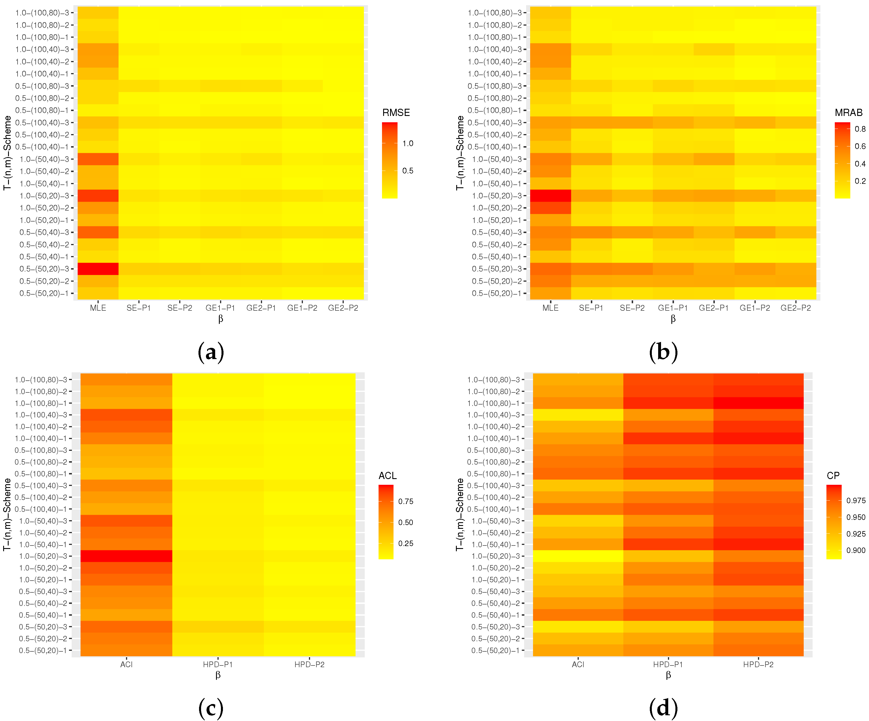
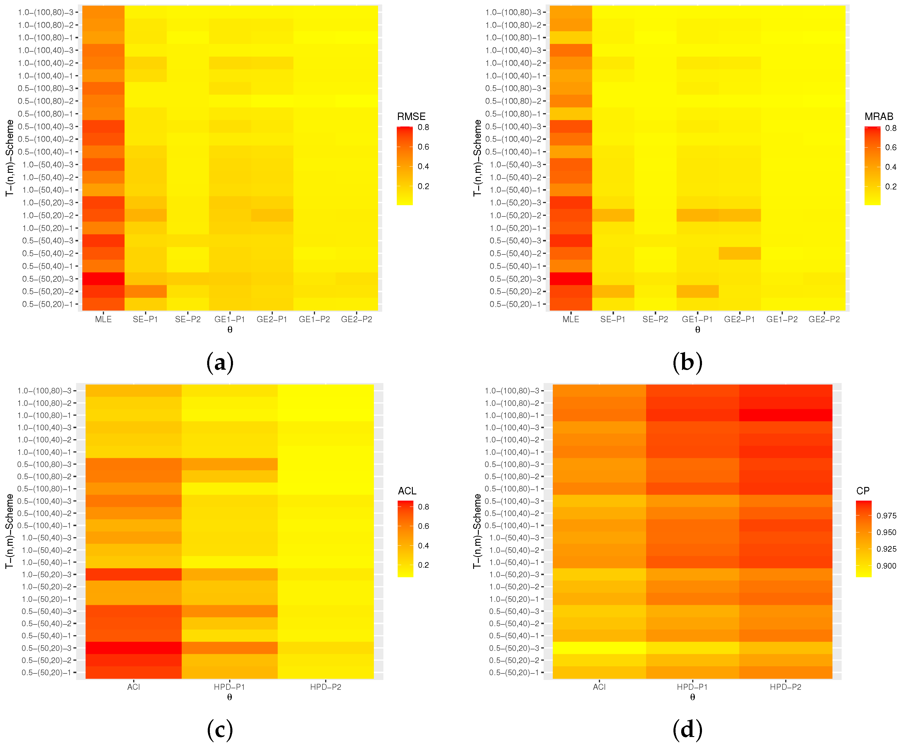
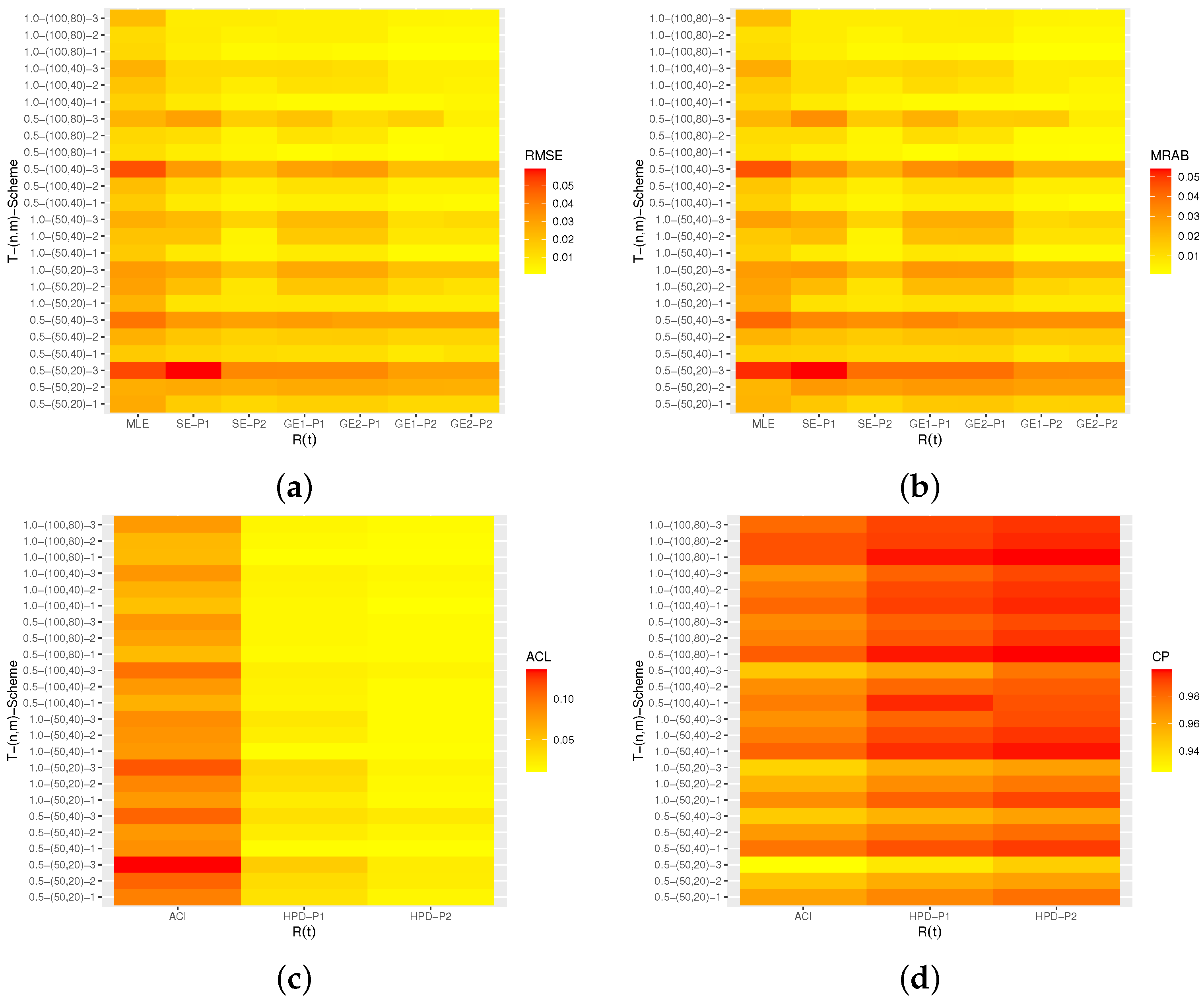
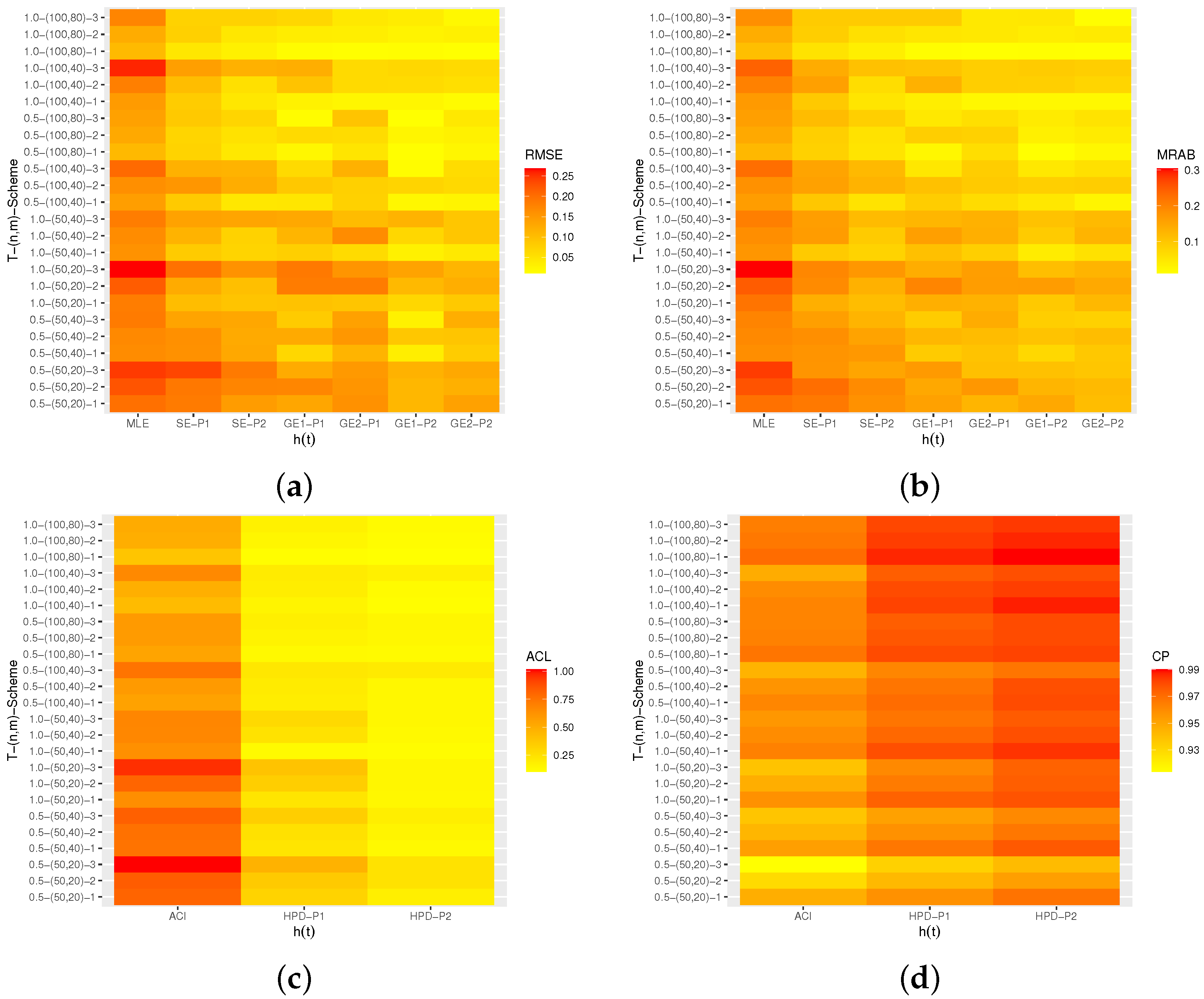
and +2 (mentioned as ‘‘GE1-P1’’ and ‘‘GE2-P1’’, respectively), and the HPD Bayes credible interval estimates (referenced as ‘‘HPD-P1’’). From Figure 1, Figure 2, Figure 3 and Figure 4, in terms of RMSEs, MRABs, ACLs, and CPs, the following conclusions about the different estimates can be stated.
  • All estimates perform better with an increase in the total (or effective) sample size. A similar performance pattern is observed when i = 1 m R i decreases.
  • The Bayes estimates of all unknown parameters have the lowest overall RMSE, MRAB, and ACL values as well as the highest CPs as compared to the frequentist estimates, as expected. Furthermore, the Bayes estimates relative to GE loss perform better than those based on SE loss.
  • The Bayes (point/interval) estimates based on Prior-2 perform more satisfactorily than those developed based on Prior-1. This is because Prior-2 has a smaller variance than Prior-1.
  • As T increases in the point estimation, it can be seen that (i) the RMSEs and MRABs decrease for θ , R ( t ) , and h ( t ) and (ii) the RMSEs and MRABs increase for β in the case of likelihood estimation and decrease in the case of Bayesian estimation.
  • As T increases in the interval estimation, it can be observed that (i) the ACLs decrease for θ , R ( t ) , and h ( t ) , whereas the associated CPs increase and (ii) the ACLs increase for β when using the ACIs and decrease in the case of HPD Bayes credible intervals.
  • Comparing Schemes 1–3, it can be noted that the point/interval estimates of β , θ , R ( t ) , and h ( t ) obtained based on Scheme 1 are more efficient than those computed using the other schemes in terms of their RMSE, MRAB, ACL, and CP values.
  • In summary, the Bayesian approach to estimating the unknown parameters and/or the reliability characteristics of the NH based on AP-II-HC samples is recommended.

5. Real-Life Applications

This section presents the analysis of two real data sets from the clinical and engineering fields to illustrate the importance and usage of the proposed methodologies in real practical situations.

5.1. Malignant Tumors

This application analyzes the survival data of 39 patients with malignant tumors of the sternum (MTS) taken from Daniel and Cross [24]. They classified patients into two groups, namely, 25 patients with low-grade MTS and 14 patients with high-grade MTS. The months (time-to-event) for patients are arranged as follows: 0, 2, 3, 4, 6, 6, 7, 8, 9, 9, 11, 12, 15, 15, 16, 17, 21, 23, 26, 27, 29, 33, 34, 75, 79, 82, 95, 102, 109, 109, 117, 122, 127, 129, 137, 138, 156, 212, 337.
To check the validity of the NH distribution for MTS data, the Kolmogorov–Smirnov (KS) statistic (along its P-value) is calculated. To perform the KS test, we first obtain the MLEs β ^ and θ ^ of β and θ (along their standard errors (St.Es)) as 0.5811 (0.1747) and 0.0435 (0.0276), respectively. However, the KS distance is 0.144 with P-value 0.391. Therefore, it stands to reason that the NH distribution fits the MTS data quite well. To examine the existence and uniqueness of the MLEs, the contour plot of the log-likelihood function for β and θ based on the MTS data set is depicted in Figure 5a. The plot indicates that the MLEs β ^ and θ ^ exist and are unique. Furthermore, Figure 5a shows that the most suitable starting values of β and θ are close to 0.5811 and 0.0435, respectively. The plots of the fitted and empirical RFs are provided in Figure 5b.
From the complete MTS data set, different AP-II-HC samples are generated using different choices of m, T, and R, and are listed in Table 1. For brevity, scheme ( R 1 , R 2 , , R m ) is used as S m : n . Using the M-H algorithm steps described in Section 3, we generate 50,000 MCMC samples and discard the first 10,000 samples.
Because prior knowledge about the NH parameters β and θ is not available, the Bayes estimates of β , θ , R ( t ) or h ( t ) at time t = 10 based on non-informative priors are obtained relative to the SE and GE (for ρ = ( 3 , 0.03 , + 3 ) ) loss functions. Moreover, utilizing 40,000 MCMC samples, the HPD Bayes credible intervals of the unknown parameters are computed. The MLEs and Bayes estimates with their St.Es of β , θ , R ( t ) , and h ( t ) are obtained and displayed in Table 2, indicating that in terms of the lowest St.Es, the Bayes estimates of β , θ , R ( t ) , and h ( t ) perform better than those obtained based on the maximum likelihood approach. In addition, the two-sided 95% ACI/HPD interval estimates along with their interval lengths (ILs) are calculated, and are presented in Table 3. The table shows that the interval estimates of β , θ , R ( t ) , and h ( t ) obtained by the asymptotic and HPD methods are quite close to each other, as expected. To examine the convergence of MCMC outputs, we use S 1 18 : 38 data as an example; the trace plots for 40,000 MCMC simulated variates of each unknown parameter are plotted in Figure 6a and Figure 6b, respectively.
Consequently, certain vital measures of MCMC samples for β , θ , R ( t ) , and h ( t ) , namely, the mean, mode, quartiles ( Q 1 , Q 2 , Q 3 ), standard deviation (St.D), and skewness are computed, and are reported in Table 4. Using the Gaussian kernel density, the corresponding histograms for 40,000 MCMC values of β , θ , R ( t ) , and h ( t ) are represented in Figure 6 as well. In each trace plot, the sample mean is represented as a solid blue line, the two bounds of the 95% HPD credible intervals are represented as dashed lines, and in each histogram plot the sample mean is shown as a red vertical dash-dotted line. Figure 6 indicates that the MCMC procedure utilizing the M-H algorithm converges satisfactorily and that the generated posterior estimates are very close to symmetric.

5.2. Sodium Sulphur Batteries

This application analyzes the lifetimes (in cycles) of sodium sulphur batteries (SSBs), and is taken from Phillips [25]. The failure times (where + represents right-censored data) of 20 SSB are as follows: 76, 82, 210, 315, 385, 412, 491, 504, 522, 646+, 678, 775, 884, 1131, 1446. The same has recently been analyzed by Alotaibi et al. [17]. First, we ignore the observation ‘646+’ (which was still running) and divide each time point in the SSB data by one hundred for the sake of computational convenience. Next, we verify whether or not the NH distribution is a suitable model to fit the SSB data. From the SSB dataset, the MLEs β ^ and θ ^ (with their St.Es) of β and θ are 1.9912 (2.1140) and 0.0381 (0.0532), respectively. Consequently, the calculated KS distance is 0.108 with P-value 0.954. This implies that the NH distribution fits the SSB data quite satisfactorily. The contour plot of the log-likelihood function of β and θ is shown in Figure 7a. The plot shows that the best initial guesses values of β and θ are quite close to 0.652 and 0.475, respectively. In addition, it shows that the acquired MLEs β ^ and θ ^ exist and are unique. In addition, the fitted and empirical RFs are displayed in Figure 7b.
Next, three different AP-II-HC samples are generated from the complete SSB data; these are presented in Table 5. Using Table 5, both the classical and Bayes estimates (with their St.Es) as well as the ACI/HPD credible interval estimates (with their ILs) of β , θ , R ( t ) , and h ( t ) at specified time t = 0.01 are calculated, and are reported in Table 6 and Table 7. Using the M-H algorithm, we generate 50,000 MCMC samples and ignore the first 10,000 samples. It is important to mention here that the Bayes estimates based on the GE loss function are obtained using the same values for ρ as in the first application.
From Table 6 and Table 7 it can be seen that the Bayes (point/interval) estimates have better performance than the frequentist estimates. Moreover, the trace and histogram plots for 40,000 MCMC estimates of β , θ , R ( t ) , and h ( t ) for S 1 10 : 20 are shown in Figure 8a,b, respectively, as an example. The plots indicate that the MCMC procedure converges very completely. In addition, it stands to reason that the posterior histograms are fairly symmetrical. Furthermore, from the S 1 10 : 20 and S 1 15 : 20 datasets, several vital statistics of the simulated MCMC variates for β , θ , R ( t ) , and h ( t ) can be computed, and are listed in Table 8.
The analysis of these two real datasets shows that the NH distribution is an accurate model for fitting the considered data. Moreover, the following findings can be observed regarding the flexibility of the AP-II-HC scheme: (1) it is adaptable and very useful in terminating the experiment when the researcher’s primary consideration is the number of failures; (2) it can preserve the duration of the experiment; and (3) satisfactory estimates of the RF and HRF can be acquired using the proposed scheme instead of using the whole sample, avoiding the need for additional time, expenses, and human resources. Ultimately, the Bayes MCMC procedure is recommended for estimating the unknown parameters of the NH model in the case of AP-II-HC data.

6. Concluding Remarks

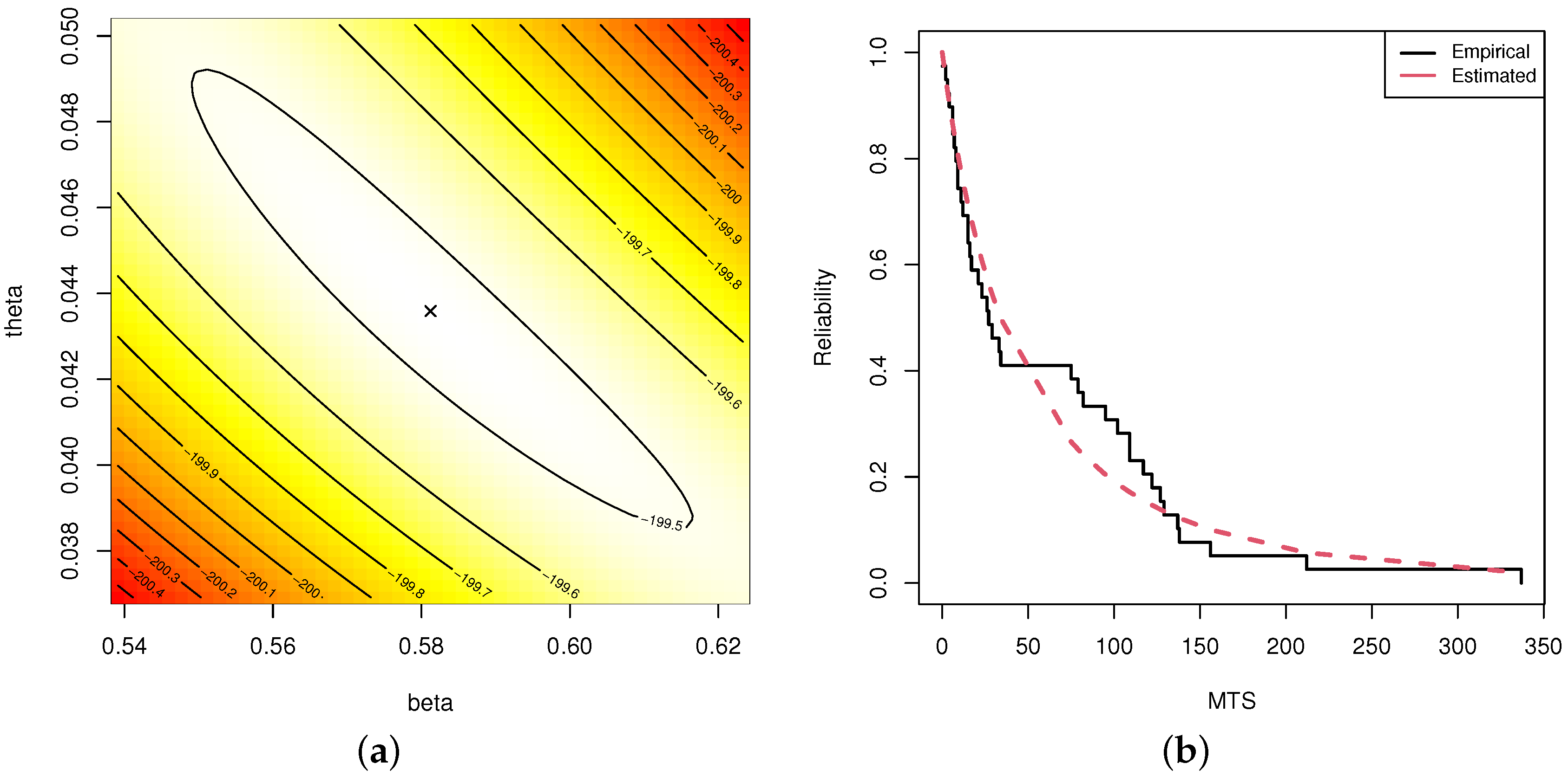
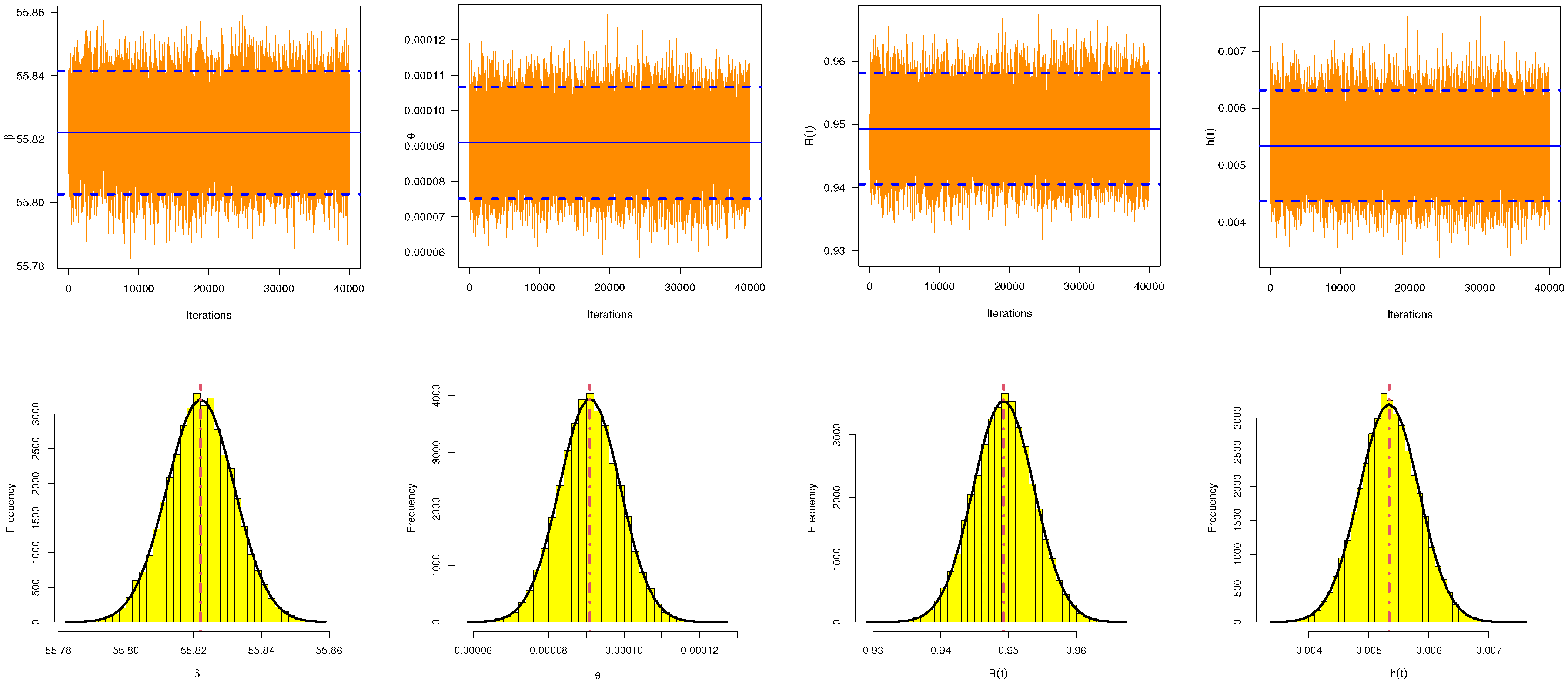
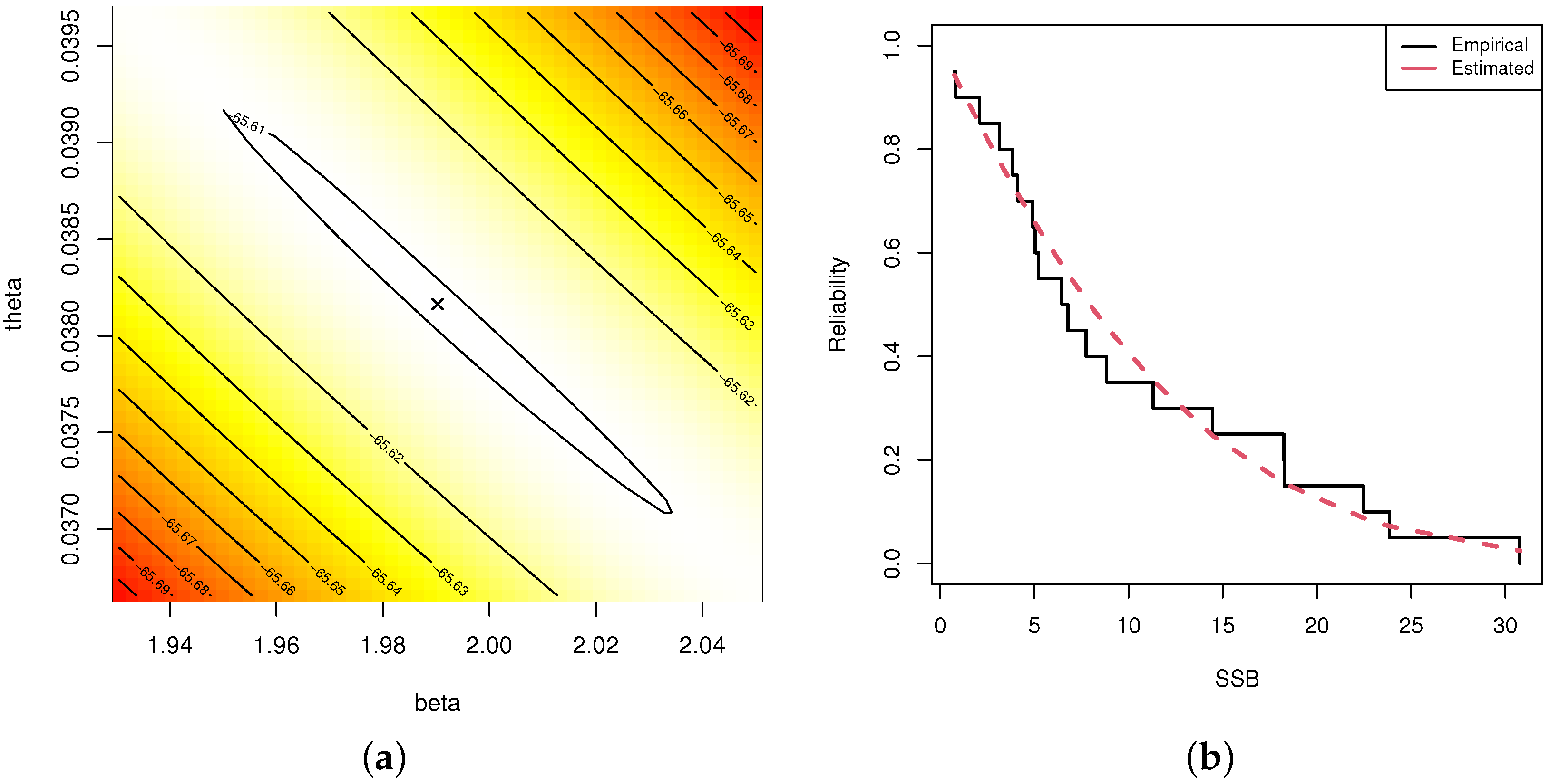
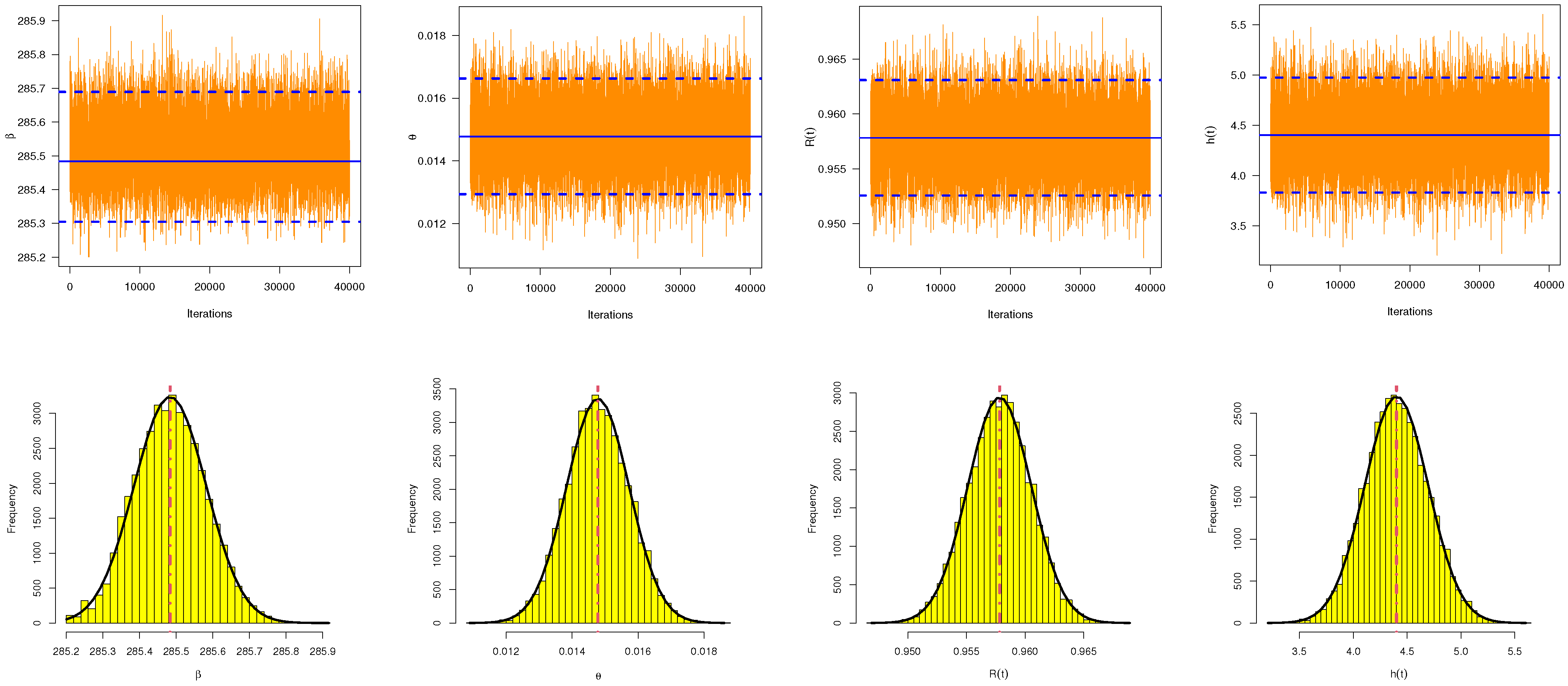
In this paper, we have investigated maximum likelihood and Bayesian inference for the Nadarajah–Haghighi distribution based on an adaptive progressive Type II censoring scheme. Due to the complex forms of the maximum likelihood equations, the maximum likelihood estimates of the unknown parameters are obtained through numerical methods. Based on the invariance property of the maximum likelihood estimates, the estimates of the reliability and hazard rate functions are derived as well. Utilizing the asymptotic properties of the maximum likelihood estimates, both the approximate confidence intervals of the unknown parameters and the reliability and hazard rate functions are acquired. On the other hand, we evaluate Bayesian estimation using two loss functions, namely, the squared error and general entropy loss functions, with the estimates obtained via the Monte Carlo Markov Chain technique. Meanwhile, we establish the highest posterior density Bayes credible intervals of the different unknown parameters. To check the performance of the various estimates, we carried out a simulation study. In the simulation part of this paper, the average values of the root mean square errors and relative absolute biases are computed to examine the performance of the point estimates, while the average interval lengths and coverage probabilities are evaluated for the interval estimates. Based on the simulation outcomes, it is evident that Bayesian estimation, which retains appropriate informative priors, is more reasonable than the maximum likelihood estimates in all cases. To be more specific, the Bayesian estimates using the general entropy loss function perform better than all other estimates. In addition, the highest posterior density Bayes credible intervals possess the smallest average interval lengths with the highest coverage probabilities when compared with the approximate confidence intervals. Finally, two real datasets, one involving patients with malignant tumors of the sternum and one involving sodium sulphur batteries, are analyzed in order to demonstrate the practicality of the different studied methodologies. In future work, it may prove essential to extend the proposed methods to include the competing risks model or accelerated life tests.

Supplementary Materials

The following supporting information can be downloaded at: https://www.mdpi.com/article/10.3390/math10203775/s1, Table S1: The RMSEs (1st column) and MRABs (2nd column) of β ; Table S2: The RMSEs (1st column) and MRABs (2nd column) of θ ; Table S3: The RMSEs (1st column) and MRABs (2nd column) of R ( t ) ; Table S4: The RMSEs (1st column) and MRABs (2nd column) of h ( t ) ; Table S5: The ACLs (1st column) and CPs (2nd column) of ACI/HPD credible intervals of β ; Table S6: The ACLs (1st column) and CPs (2nd column) of ACI/HPD credible intervals of θ ; Table S7: The ACLs (1st column) and CPs (2nd column) of ACI/HPD credible intervals of R ( t ) ; Table S8: The ACLs (1st column) and CPs (2nd column) of ACI/HPD credible intervals of h ( t ) .

Author Contributions

Methodology, R.A. and M.N.; Funding acquisition, R.A.; Software, A.E.; Supervision, M.N. and A.E.; Writing—original draft, R.A. and A.E.; Writing—review and editing, R.A. and M.N. All authors have read and agreed to the published version of the manuscript.

Funding

This research was funded by Princess Nourah bint Abdulrahman University Researchers Supporting Project No. PNURSP2022R50, Princess Nourah bint Abdulrahman University, Riyadh, Saudi Arabia.

Data Availability Statement

The authors confirm that the data supporting the findings of this study are available within the article.

Acknowledgments

The authors wish to express their gratitude to the editor and the three anonymous referees for their valuable recommendations and beneficial comments, as well as for the financial support provided by Princess Nourah bint Abdulrahman University Researchers Supporting Project No. PNURSP2022R50, Princess Nourah bint Abdulrahman University, Riyadh, Saudi Arabia.

Conflicts of Interest

The authors declare no conflict of interest.

Abbreviations

The following abbreviations are used in this article:
ACIApproximate Confidence Interval
MLEMaximum Likelihood Estimator
ACLAverage Confidence Length
MRABMean Relative Absolute Bias
AP-II-HCAdaptive Progressive Type-II Hybrid Censoring
MTSMalignant Tumors of the Sternum
CDFCumulative Distribution Function
NHNadarajah–Haghighi
CPCoverage Percentage
PDFProbability Density Function
GEGeneral Entropy
PT-II-CSProgressive Type-II Censoring Scheme
HPDHighest Posterior Density
RFReliability Function
HRFHazard Rate Function
RMSERoot Mean Square Error
ILInterval Length
SESquared Error
KSKolmogorov–Smirnov
SSBSodium Sulphur Battery
MCMCMonte Carlo Markov Chain
St.DStandard Deviation
M-HMetropolis–Hastings
St.EStandard Error

References

  1. Nadarajah, S.; Haghighi, F. An extension of the exponential distribution. Statistics 2011, 45, 543–558. [Google Scholar] [CrossRef]
  2. Mohie El-Din, M.M.; Abu-Youssef, S.E.; Ali, N.S.; Abd El-Raheem, A.M. Estimation in constant-stress accelerated life tests for extension of the exponential distribution under progressive censoring. Metron 2016, 74, 253–273. [Google Scholar] [CrossRef]
  3. Mohie El-Din, M.M.; Abu-Youssef, S.E.; Ali, N.S.; Abd El-Raheem, A.M. Classical and Bayesian inference on progressive-stress accelerated life testing for the extension of the exponential distribution under progressive Type-II censoring. Qual. Reliab. Eng. Int. 2017, 33, 2483–2496. [Google Scholar] [CrossRef]
  4. Dey, S.; Zhang, C.; Asgharzadeh, A.; Ghorbannezhad, M. Comparisons of methods of estimation for the NH distribution. Ann. Data Sci. 2017, 4, 441–455. [Google Scholar] [CrossRef]
  5. Selim, M.A. Estimation and prediction for Nadarajah-Haghighi distribution based on record values. Pak. J. Statist. 2018, 34, 77–90. [Google Scholar] [CrossRef]
  6. Ashour, S.K.; El-Sheikh, A.A.; Elshahhat, A. Inferences and optimal censoring schemes for progressively first-failure censored Nadarajah-Haghighi distribution. Sankhya A 2022, 84, 885–923. [Google Scholar] [CrossRef]
  7. Balakrishnan, N.; Aggarwala, R. Progressive Censoring Theory, Methods and Applications; Birkhäuser: Boston, MA, USA, 2000. [Google Scholar]
  8. Balakrishnan, N. Progressive censoring methodology: An appraisal (with discussions). Test 2007, 16, 211–296. [Google Scholar] [CrossRef]
  9. Kundu, D.; Joarder, A. Analysis of Type-II progressively hybrid censored data. Comput. Stat. Data Anal. 2006, 50, 2509–2528. [Google Scholar] [CrossRef]
  10. Ng, H.K.T.; Kundu, D.; Chan, P.S. Statistical Analysis of Exponential Lifetimes under an Adaptive Type-II Progressive Censoring Scheme. Nav. Res. Logist. 2009, 56, 687–698. [Google Scholar] [CrossRef] [Green Version]
  11. Nassar, M.; Abo-Kasem, O.E. Estimation of the inverse Weibull parameters under adaptive Type-II progressive hybrid censoring scheme. J. Comput. Appl. Math. 2017, 315, 228–239. [Google Scholar] [CrossRef]
  12. Ateya, S.F.; Mohammed, H.S. Statistical inferences based on an adaptive progressive Type-II censoring from exponentiated exponential distribution. J. Egypt. Math. Soc. 2017, 25, 393–399. [Google Scholar] [CrossRef]
  13. Mohie El-Din, M.M.M.; Amein, M.M.; Shafay, A.R.; Mohamed, S. Estimation of generalized exponential distribution based on an adaptive progressively Type-II censored sample. J. Stat. Comput. Simul. 2017, 87, 1292–1304. [Google Scholar] [CrossRef]
  14. Liu, S.; Gui, W. Estimating the parameters of the two-parameter Rayleigh distribution based on adaptive Type II progressive hybrid censored data with competing risks. Mathematics 2020, 8, 1783. [Google Scholar] [CrossRef]
  15. Elshahhat, A.; Nassar, M. Bayesian survival analysis for adaptive Type-II progressive hybrid censored Hjorth data. Comput. Stat. 2021, 36, 1965–1990. [Google Scholar] [CrossRef]
  16. Kohansal, A.; Bakouch, H.S. Estimation procedures for Kumaraswamy distribution parameters under adaptive Type-II hybrid progressive censoring. Commun. Stat.-Simul. Comput. 2021, 50, 4059–4078. [Google Scholar] [CrossRef]
  17. Alotaibi, R.; Nassar, M.; Elshahhat, A. Computational Analysis of XLindley Parameters Using Adaptive Type-II Progressive Hybrid Censoring with Applications in Chemical Engineering. Mathematics 2022, 10, 3355. [Google Scholar] [CrossRef]
  18. Martz, H.F.; Waller, R.A. Bayesian Reliability Analysis; Wiley and Sons: New York, NY, USA, 1982. [Google Scholar]
  19. Dey, D.K.; Ghosh, M.; Srinivasan, C. Simultaneous estimation of parameters under entropy loss. J. Stat. Plan. Inference 1987, 15, 347–363. [Google Scholar] [CrossRef]
  20. Chen, M.H.; Shao, Q.M. Monte Carlo estimation of Bayesian credible and HPD intervals. J. Comput. Graph. Stat. 1999, 8, 69–92. [Google Scholar]
  21. Balakrishnan, N.; Sandhu, R.A. A simple simulational algorithm for generating progressive Type-II censored samples. Am. Stat. 1995, 49, 229–230. [Google Scholar]
  22. Henningsen, A.; Toomet, O. maxLik: A package for maximum likelihood estimation in R. Comput. Stat. 2011, 26, 443–458. [Google Scholar] [CrossRef]
  23. Plummer, M.; Best, N.; Cowles, K.; Vines, K. CODA: Convergence diagnosis and output analysis for MCMC. R News 2006, 6, 7–11. [Google Scholar]
  24. Daniel, W.W.; Cross, C.L. Biostatistics: A Foundation for Analysis in the Health Sciences, 10th ed.; John Wiley and Sons: Hoboken, NJ, USA, 2018. [Google Scholar]
  25. Phillips, M.J. Statistical Methods for Reliability Data Analysis. In Handbook of Reliability Engineering; Springer: London, UK, 2003. [Google Scholar]
Figure 1. Heatmap plots for the estimation results of β . (a) RMSE. (b) MRAB. (c) ACL. (d) CP.
Mathematics 10 03775 g001
Figure 2. Heatmap plots for the estimation results of θ . (a) RMSE. (b) MRAB. (c) ACL. (d) CP.
Mathematics 10 03775 g002
Figure 3. Heatmap plots for the estimation results of R ( t ) . (a) RMSE. (b) MRAB. (c) ACL. (d) CP.
Mathematics 10 03775 g003
Figure 4. Heatmap plots for the estimation results of h ( t ) . (a) RMSE. (b) MRAB. (c) ACL. (d) CP.
Mathematics 10 03775 g004
Figure 5. (a) Contour plot of β and θ and (b) fitted/empirical RFs (right panel) from MTS data.
Mathematics 10 03775 g005
Figure 6. Trace (top panel) and Histogram (bottom panel) plots of β , θ , R ( t ) , and h ( t ) under MTS data.
Mathematics 10 03775 g006
Figure 7. (a) Contour plot of β and θ and (b) fitted/empirical RFs (right panel) from SSB data.
Mathematics 10 03775 g007
Figure 8. Trace (top panel) and Histogram (bottom panel) plots of β , θ , R ( t ) , and h ( t ) under SSB data.
Mathematics 10 03775 g008
Table 1. Different AP-II-HC samples from MTS data.
S i m : n mScheme T ( d ) R m Generated Sample
S 1 18 : 38 18 ( 20 , 0 * 17 ) 80 (4)02, 34, 75, 79, 82, 95, 102, 109, 109, 117, 122, 127, 129, 137, 138, 156, 212, 337
S 2 18 : 38 18 ( 0 * 4 , 2 * 10 , 0 * 4 ) 30 (10)82, 3, 4, 6, 6, 9, 12, 16, 23, 29, 75, 79, 82, 95, 102, 109, 109, 117
S 3 18 : 38 18 ( 0 * 17 , 20 ) 10 (12)02, 3, 4, 6, 6, 7, 8, 9, 9, 11, 12, 15, 15, 16, 17, 21, 23, 26, 27, 29
S 1 28 : 38 28 ( 10 , 0 * 27 ) 100 (16)02, 15, 15, 16, 17, 21, 23, 26, 27, 29, 33, 34, 75, 79, 82, 95, 102, 109, 109, 117, 122,
127, 129, 137, 138, 156, 212, 337
S 2 28 : 38 28 ( 0 * 9 , 1 * 10 , 0 * 9 ) 30 (15)42, 3, 4, 6, 6, 7, 8, 9, 9, 11, 15, 16, 21, 26, 29, 34, 75, 79, 82, 95, 102, 109, 109, 117,
122, 127, 129, 137
S 3 28 : 38 28 ( 0 * 27 , 10 ) 20 (15)02, 3, 4, 6, 6, 7, 8, 9, 9, 11, 12, 15, 15, 16, 17, 21, 23, 26, 27, 29, 33, 34, 75, 79, 82,
95, 102, 109
* represents number of repeated times for zeros.
Table 2. The point estimates (St.Es) of β , θ , R ( t ) , and h ( t ) under MTS data.
S i m : n
ρ
Par.MLESEGE
3 0.03 +3
S 1 18 : 38 β 55.8232 (0.90 × 10 + 1 )55.8221 (4.97 × 10 5 )55.8220 (9.40 × 10 4 )55.8221 (4.97 × 10 5 )55.8221 (9.45 × 10 5 )
θ 0.00009 (2.07 × 10 5 )0.00009 (4.03 × 10 8 )0.00009 (1.63 × 10 6 )0.00009 (5.66 × 10 7 )0.00009 (5.59 × 10 7 )
R ( 10 ) 0.94727 (7.59 × 10 3 )0.94929 (2.24 × 10 5 )0.94931 (4.88 × 10 4 )0.94928 (5.19 × 10 4 )0.94925 (5.52 × 10 4 )
h ( 10 ) 0.00556 (8.43 × 10 4 )0.00534 (2.49 × 10 6 )0.00538 (1.05 × 10 4 )0.00531 (3.59 × 10 5 )0.00524 (3.68 × 10 5 )
S 2 18 : 38 β 56.2524 (0.55 × 10 + 1 )56.2510 (4.98 × 10 5 )56.2510 (9.69 × 10 4 )56.2510 (9.71 × 10 4 )56.2510 (9.74 × 10 4 )
θ 0.00011 (2.29 × 10 5 )0.00010 (4.42 × 10 8 )0.00010 (2.84 × 10 6 )0.00010 (1.71 × 10 6 )0.00010 (5.15 × 10 7 )
R ( 10 ) 0.93659 (1.11 × 10 2 )0.94264 (2.48 × 10 5 )0.94267 (1.14 × 10 3 )0.94263 (1.18 × 10 3 )0.94259 (1.22 × 10 3 )
h ( 10 ) 0.00676 (1.26 × 10 3 )0.00608 (2.78 × 10 6 )0.00613 (1.84 × 10 4 )0.00605 (1.08 × 10 4 )0.00597 (2.94 × 10 5 )
S 3 18 : 38 β 288.065 (0.85 × 10 + 1 )288.064 (4.95 × 10 5 )288.064 (1.01 × 10 3 )288.064 (1.01 × 10 3 )288.064 (1.02 × 10 3 )
θ 0.00016 (2.35 × 10 5 )0.00016 (4.58 × 10 8 )0.00016 (1.14 × 10 6 )0.00016 (3.67 × 10 7 )0.00016 (4.36 × 10 7 )
R ( 10 ) 0.53984 (5.76 × 10 2 )0.55575 (1.16 × 10 4 )0.55672 (4.26 × 10 4 )0.55528 (1.87 × 10 3 )0.55380 (3.35 × 10 3 )
h ( 10 ) 0.07756 (1.58 × 10 2 )0.07438 (3.06 × 10 5 )0.07399 (1.06 × 10 3 )0.07323 (3.02 × 10 4 )0.07246 (4.76 × 10 4 )
S 1 28 : 38 β 1.08092 (5.39 × 10 1 )1.08041 (4.99 × 10 5 )1.08051 (4.15 × 10 4 )1.08037 (5.52 × 10 4 )1.08023 (6.92 × 10 4 )
θ 0.00907 (7.04 × 10 3 )0.00907 (5.01 × 10 8 )0.00907 (1.71 × 10 8 )0.00907 (1.81 × 10 8 )0.00907 (3.49 × 10 8 )
R ( 10 ) 0.90626 (2.65 × 10 2 )0.90634 (4.35 × 10 6 )0.90634 (4.48 × 10 5 )0.90633 (4.35 × 10 5 )0.90634 (4.23 × 10 5 )
h ( 10 ) 0.00988 (2.78 × 10 3 )0.00987 (5.02 × 10 7 )0.00986 (3.97 × 10 6 )0.00987 (5.49 × 10 6 )0.00986 (7.04 × 10 6 )
S 2 28 : 38 β 95.8364 (0.68 × 10 + 1 )95.8355 (5.03 × 10 5 )95.8354 (9.36 × 10 4 )95.8355 (9.37 × 10 4 )95.8354 (9.39 × 10 4 )
θ 0.00008 (1.19 × 10 5 )0.00008 (3.59 × 10 8 )0.00008 (1.14 × 10 6 )0.00008 (1.93 × 10 7 )0.00008 (8.07 × 10 7 )
R ( 10 ) 0.92142 (9.91 × 10 3 )0.92296 (3.43 × 10 5 )0.92301 (4.30 × 10 4 )0.92293 (5.06 × 10 4 )0.92286 (5.83 × 10 4 )
h ( 10 ) 0.00851 (1.16 × 10 3 )0.00833 (3.39 × 10 6 )0.00841 (1.38 × 10 4 )0.00829 (2.41 × 10 5 )0.00817 (9.56 × 10 5 )
S 3 28 : 38 β 333.434 (0.42 × 10 + 1 )333.432 (4.99 × 10 5 )333.433 (1.05 × 10 3 )333.433 (1.05 × 10 3 )333.432 (1.05 × 10 3 )
θ 0.00005 (5.16 × 10 6 )0.00005 (2.30 × 10 8 )0.00005 (3.27 × 10 6 )0.00005 (3.95 × 10 6 )0.00005 (4.67 × 10 6 )
R ( 10 ) 0.84785 (1.69 × 10 2 )0.84640 (7.56 × 10 5 )0.84667 (1.25 × 10 2 )0.84627 (1.21 × 10 2 )0.84586 (1.17 × 10 2 )
h ( 10 ) 0.01779 (2.29 × 10 3 )0.01802 (1.03 × 10 5 )0.01826 (1.43 × 10 3 )0.01791 (1.78 × 10 3 )0.01754 (2.15 × 10 3 )
Table 3. The 95% interval estimates (ILs) of β , θ , R ( t ) , and h ( t ) under MTS data.
S i m : n Par.ACIHPD
S 1 18 : 38 β (38.1642, 73.4822) [35.3180](55.8026, 55.8415) [0.38946]
θ (0.00005, 0.00014) [0.00009](0.00008, 0.00011) [0.00003]
R ( 10 ) (0.93238, 0.96216) [0.02978](0.94051, 0.95814) [0.01763]
h ( 10 ) (0.00391, 0.00721) [0.00331](0.00436, 0.00631) [0.00195]
S 2 18 : 38 β (45.2941, 67.2107) [21.9166](56.2316, 56.2706) [0.03897]
θ (0.00007, 0.00016) [0.00009](0.00008, 0.00012) [0.00004]
R ( 10 ) (0.91481, 0.95836) [0.04355](0.93264, 0.95218) [0.01954]
h ( 10 ) (0.00429, 0.00923) [0.00494](0.00500, 0.00719) [0.00219]
S 3 18 : 38 β (271.236, 304.893) [33.6565](288.045, 288.084) [0.03870]
θ (0.00012, 0.00021) [0.00009](0.00014, 0.00018) [0.00004]
R ( 10 ) (0.42684, 0.65284) [0.22599](0.51020, 0.60110) [0.09090]
h ( 10 ) (0.04662, 0.10851) [0.06188](0.06155, 0.08546) [0.02391]
S 1 28 : 38 β (0.02448, 2.13736) [2.11288](1.06087, 1.10005) [0.03918]
θ (0.00472, 0.02287) [0.01815](0.00905, 0.00909) [0.00004]
R ( 10 ) (0.85418, 0.95834) [0.10416](0.90461, 0.90801) [0.00340]
h ( 10 ) (0.00441, 0.01534) [0.01093](0.00967, 0.01006) [0.00039]
S 2 28 : 38 β (82.4225, 109.250) [26.8278](95.8162, 95.8555) [0.03933]
θ (0.00006, 0.00011) [0.00005](0.00006, 0.00009) [0.00003]
R ( 10 ) (0.90198, 0.94086) [0.03887](0.90959, 0.93639) [0.02680]
h ( 10 ) (0.00623, 0.01078) [0.00455](0.00679, 0.00991) [0.00312]
S 3 28 : 38 β (325.159, 341.709) [16.5508](333.413, 333.452) [0.03901]
θ (0.00004, 0.00005) [0.00001](0.00003, 0.00006) [0.00003]
R ( 10 ) (0.81477, 0.88094) [0.06617](0.81596, 0.87503) [0.05907]
h ( 10 ) (0.01329, 0.02229) [0.00899](0.01395, 0.02201) [0.00806]
Table 4. Vital measures of MCMC outputs of β , θ , R ( t ) , and h ( t ) under MTS data.
S i m : n Par.MeanMode Q 1 Q 2 Q 3 St.DSkewness
S 1 18 : 38 β 55.8220655.8052655.8153055.8220455.828831.00 × 10 2 −0.000361
θ 0.0000910.0000880.0000850.0000910.0000968.02 × 10 6 −0.012473
R ( 10 ) 0.9493040.9507240.9463090.9492910.9522894.47 × 10 3 +0.013413
h ( 10 ) 0.0053350.0051760.0050040.0053340.0056654.94 × 10 4 +0.012804
S 1 28 : 38 β 1.0804131.0631061.0736911.0803931.0871159.98 × 10 3 +0.021721
θ 0.0090690.0090450.0090630.0090690.0090771.00 × 10 5 +0.005913
R ( 10 ) 0.9063390.9074320.9057550.9063420.9069228.70 × 10 4 −0.0215269
h ( 10 ) 0.0098680.0096910.0098010.0098670.0099351.00 × 10 4 +0.026774
Table 5. Different AP-II-HC samples from SSB data.
S i m : n mScheme T ( d ) R m Generated Sample
S 1 10 : 20 10 ( 10 , 0 * 9 ) 0.3 (9)00.0076, 0.0775, 0.0884, 0.1131, 0.1446, 0.1824, 0.1827, 0.2248, 0.2385, 0.3077
S 2 10 : 20 10 ( 0 * 3 , 2 * 5 , 0 * 2 ) 0.1 (7)20.0076, 0.0082, 0.0210, 0.0315, 0.0491, 0.0646, 0.0884, 0.1824, 0.1827, 0.2248
S 3 10 : 20 10 ( 0 * 9 , 10 ) 0.05 (7)00.0076, 0.0082, 0.0210, 0.0315, 0.0385, 0.0412, 0.0491, 0.0504, 0.0522, 0.0646
S 1 15 : 20 15 ( 5 , 0 * 14 ) 0.2 (12)00.0076, 0.0491, 0.0504, 0.0522, 0.0646, 0.0678, 0.0775, 0.0884, 0.1131, 0.1446,
0.1824, 0.1827, 0.2248, 0.2385, 0.3077
S 2 15 : 20 15 ( 0 * 5 , 1 * 5 , 0 * 5 ) 0.06 (7)30.0076, 0.0082, 0.0210, 0.0315, 0.0385, 0.0412, 0.0504, 0.0646, 0.0678, 0.0775,
0.0884, 0.1131, 0.1446, 0.1824, 0.1827
S 3 15 : 20 15 ( 0 * 14 , 5 ) 0.04 (5)00.0076, 0.0082, 0.0210, 0.0315, 0.0385, 0.0412, 0.0491, 0.0504, 0.0522, 0.0646,
0.0678, 0.0775, 0.0884, 0.1131, 0.1446
* represents number of repeated times for zeros.
Table 6. The point estimates (St.Es) of β , θ , R ( t ) , and h ( t ) under SSB data.
S i m : n
ρ
Par.MLESEGE
3 0.03 +3
S 1 10 : 20 β 285.582 (2.61 × 10 + 1 )285.483 (4.92 × 10 4 )285.484 (9.84 × 10 2 )285.484 (9.84 × 10 2 )285.483 (9.85 × 10 2 )
θ 0.01484 (3.25 × 10 3 )0.01478 (4.75 × 10 6 )0.01484 (1.50 × 10 6 )0.01475 (8.93 × 10 5 )0.01466 (1.83 × 10 4 )
R ( 0.01 ) 0.95763 (8.42 × 10 3 )0.95782 (1.36 × 10 5 )0.95783 (1.92 × 10 4 )0.95781 (1.80 × 10 4 )0.95780 (1.69 × 10 4 )
h ( 0.01 ) 4.42139 (9.16 × 10 1 )4.40158 (1.47 × 10 3 )4.42128 (4.44 × 10 4 )4.39195 (2.89 × 10 3 )4.36157 (5.92 × 10 2 )
S 2 10 : 20 β 137.074 (0.19 × 10 + 1 )136.974 (4.98 × 10 4 )136.975 (9.94 × 10 2 )136.974 (9.95 × 10 2 )136.974 (9.97 × 10 2 )
θ 0.02921 (7.93 × 10 3 )0.02915 (4.97 × 10 6 )0.02918 (2.19 × 10 5 )0.02914 (7.23 × 10 5 )0.02909 (1.24 × 10 4 )
R ( 0.01 ) 0.95998 (9.17 × 10 3 )0.96008 (6.81 × 10 6 )0.96008 (1.07 × 10 4 )0.96008 (1.04 × 10 4 )0.96007 (1.02 × 10 4 )
h ( 0.01 ) 4.16559 (9.93 × 10 1 )4.15505 (7.38 × 10 4 )4.16028 (5.98 × 10 3 )4.15250 (1.38 × 10 2 )4.14452 (2.17 × 10 2 )
S 3 10 : 20 β 385.152 (0.17 × 10 + 1 )385.050 (4.99 × 10 4 )385.050 (1.02 × 10 1 )385.050 (1.02 × 10 1 )385.050 (1.02 × 10 1 )
θ 0.04924 (9.98 × 10 3 )0.04922 (4.99 × 10 6 )0.04924 (2.47 × 10 6 )0.04921 (2.76 × 10 5 )0.04918 (5.84 × 10 5 )
R ( 0.01 ) 0.81156 (3.68 × 10 2 )0.81170 (1.89 × 10 5 )0.81172 (1.35 × 10 4 )0.81169 (1.09 × 10 4 )0.81167 (8.29 × 10 5 )
h ( 0.01 ) 22.9162 (0.53 × 10 + 1 )22.8977 (2.76 × 10 3 )22.9111 (1.79 × 10 3 )22.8913 (2.16 × 10 2 )22.8711 (4.18 × 10 2 )
S 1 15 : 20 β 132.062 (0.28 × 10 + 1 )131.962 (4.94 × 10 4 )131.962 (9.98 × 10 2 )131.962 (9.99 × 10 2 )131.961 (1.00 × 10 1 )
θ 0.03736 (9.97 × 10 3 )0.03734 (4.99 × 10 6 )0.03736 (8.62 × 10 6 )0.03732 (3.09 × 10 5 )0.03729 (7.15 × 10 5 )
R ( 0.01 ) 0.95069 (7.82 × 10 3 )0.95075 (6.57 × 10 6 )0.95075 (6.29 × 10 5 )0.95075 (6.02 × 10 5 )0.95074 (5.75 × 10 5 )
h ( 0.01 ) 5.18145 (8.63 × 10 1 )5.17483 (7.25 × 10 4 )5.17889 (2.49 × 10 3 )5.17286 (8.53 × 10 3 )5.16668 (1.47 × 10 2 )
S 2 15 : 20 β 497.492 (0.12 × 10 + 1 )497.391 (4.98 × 10 4 )497.391 (1.01 × 10 1 )497.391 (1.01 × 10 1 )497.391 (1.00 × 10 1 )
θ 0.01108 (1.96 × 10 3 )0.01100 (4.42 × 10 6 )0.01107 (5.10 × 10 6 )0.01097 (1.11 × 10 4 )0.01086 (2.22 × 10 4 )
R ( 0.01 ) 0.94491 (9.67 × 10 3 )0.94530 (2.21 × 10 5 )0.94532 (4.12 × 10 4 )0.94529 (3.81 × 10 4 )0.94526 (3.50 × 10 4 )
h ( 0.01 ) 5.82417 (0.11 × 10 1 )5.78243 (2.46 × 10 3 )5.82411 (1.87 × 10 4 )5.76199 (6.19 × 10 2 )5.69710 (1.26 × 10 1 )
S 3 15 : 20 β 522.826 (0.12 × 10 + 1 )522.726 (4.92 × 10 4 )522.726 (1.00 × 10 1 )522.725 (1.00 × 10 1 )522.726 (1.00 × 10 1 )
θ 0.02079 (3.30 × 10 3 )0.02074 (4.76 × 10 6 )0.02078 (5.68 × 10 6 )0.02072 (7.05 × 10 5 )0.02065 (1.37 × 10 4 )
R ( 0.01 ) 0.89153 (1.69 × 10 2 )0.89181 (2.47 × 10 5 )0.89184 (3.06 × 10 4 )0.89180 (2.65 × 10 4 )0.89176 (2.24 × 10 4 )
h ( 0.01 ) 12.1112 (0.21 × 10 + 1 )12.0835 (3.07 × 10 3 )12.1147 (2.99 × 10 4 )12.0683 (4.67 × 10 2 )12.0206 (9.43 × 10 2 )
Table 7. The 95% interval estimates (ILs) of β , θ , R ( t ) , and h ( t ) under SSB data.
S i m : n Par.ACIHPD
S 1 10 : 20 β (234.382, 336.782) [102.400](285.305, 285.670) [0.38477]
θ (0.00847, 0.02121) [0.01274](0.01294, 0.01663) [0.00369]
R ( 0.01 ) (0.94112, 0.97414) [0.03301](0.95257, 0.96309) [0.01052]
h ( 0.01 ) (2.62508, 6.21770) [3.59262](3.83097, 4.97490) [1.14393]
S 2 10 : 20 β (98.1428, 176.004) [77.8616](136.789, 137.176) [0.38797]
θ (0.01366, 0.04475) [0.03108](0.02720, 0.03108) [0.00388]
R ( 0.01 ) (0.94201, 0.97796) [0.03595](0.95745, 0.96277) [0.00532]
h ( 0.01 ) (2.21894, 6.11225) [3.89331](3.86419, 4.44045) [0.57627]
S 3 10 : 20 β (351.439, 418.864) [67.4256](384.841, 385.234) [0.39277]
θ (0.02968, 0.06881) [0.03913](0.04732, 0.05123) [0.00391]
R ( 0.01 ) (0.73949, 0.88363) [0.14414](0.80426, 0.81902) [0.01477]
h ( 0.01 ) (12.3565, 33.4759) [0.19304](21.7725, 23.9350) [2.16247]
S 1 15 : 20 β (76.8197, 187.304) [110.485](131.773, 132.155) [0.38239]
θ (0.01782, 0.05689) [0.03908](0.03534, 0.03927) [0.00393]
R ( 0.01 ) (0.93535, 0.96602) [0.03067](0.94819, 0.95336) [0.00517]
h ( 0.01 ) (3.48957, 6.87333) [3.38376](4.88778, 5.45809) [0.57031]
S 2 15 : 20 β (474.023, 520.962) [46.9391](497.197, 497.582) [0.38488]
θ (0.00723, 0.01493) [0.00770](0.00923, 0.01274) [0.00350]
R ( 0.01 ) (0.92595, 0.96385) [0.03790](0.93645, 0.95385) [0.01740]
h ( 0.01 ) (3.70814, 7.94020) [4.23206](4.80768, 6.74853) [1.94085]
S 3 15 : 20 β (499.327, 546.325) [46.9975](522.534, 522.915) [0.38189]
θ (0.01432, 0.02726) [0.01295](0.01893, 0.02269) [0.00376]
R ( 0.01 ) (0.85825, 0.92482) [0.06656](0.88179, 0.90129) [0.01950]
h ( 0.01 ) (7.97698, 16.2529) [8.27595](10.9142, 13.3392) [2.42500]
Table 8. Vital measures of MCMC outputs of β , θ , R ( t ) , and h ( t ) under SSB data.
S i m : n Par.MeanMode Q 1 Q 2 Q 3 St.DSkewness
S 1 10 : 20 β 285.4836285.2006285.4152285.4827285.55049.86 × 10 2 +0.073569
θ 0.0147810.0137930.0141390.0147660.0154219.51 × 10 4 +0.023780
R ( 10 ) 0.9578200.9606740.9559920.9578640.9596532.71 × 10 3 −0.023563
h ( 10 ) 4.4015754.0911524.2016304.3959604.5999312.95 × 10 1 +0.039569
S 1 15 : 20 β 131.9620131.7252131.8950131.9615132.02899.87 × 10 2 +0.043861
θ 0.0373410.0391470.0366790.0373340.0380149.98 × 10 4 −0.000245
R ( 10 ) 0.9507520.9484660.9498680.9507560.9516311.31 × 10 3 +0.000603
h ( 10 ) 5.1748305.4273825.0777525.1741715.2722761.45 × 10 1 +0.007415
Publisher’s Note: MDPI stays neutral with regard to jurisdictional claims in published maps and institutional affiliations.

