Robust Flatness-Based Tracking Control for a “Full-Bridge Buck Inverter–DC Motor” System

Abstract

By developing a robust control strategy based on the differential flatness concept, this paper presents a solution for the bidirectional trajectory tracking task in the “full-bridge Buck inverter–DC motor” system. The robustness of the proposed control is achieved by taking advantage of the differential flatness property related to the mathematical model of the system. The performance of the control, designed via the flatness concept, is verified in two ways. The first is by implementing experimentally the flatness control and proposing different shapes for the desired angular velocity profiles. For this aim, a built prototype of the “full-bridge Buck inverter–DC motor” system, along with Matlab–Simulink and a DS1104 board from dSPACE are used. The second is via simulation results, i.e., by programming the system in closed-loop with the proposed control algorithm through Matlab–Simulink. The experimental and the simulation results are similar, thus demonstrating the effectiveness of the designed robust control even when abrupt electrical variations are considered in the system.

1. Introduction

During the 21st century, the progress in energy transformation has allowed expansion of the spectrum of technological applications from a purely industrial sector to a domestic one. A clear example of such a change has been the diversification of devices that require the transformation of electric energy into mechanical energy. With the aim of accomplishing the aforesaid task of energetic transformation, one of the electric machines mainly used is the DC motor. Thus, currently there is wide use of the DC motor in applications ranging from home and public services to the entertainment industry. This fact, joined with the historical necessity of DC motors in industrial applications [1], means the research community is still interested in developing drivers for DC motors. Moreover, derived from the excellent benefits arising from feeding DC motors with power electronics converters, in the last two decades, several efforts have developed new controllers for different “DC/DC power electronic converters–DC motor” connections [2,3,4,5,6,7,8,9,10,11,12,13,14,15,16,17,18,19,20,21,22,23,24,25,26,27,28,29,30,31,32,33,34,35,36,37,38,39,40,41,42,43,44,45,46,47,48,49,50,51,52,53,54,55,56,57,58,59,60]. In particular, for the DC/DC Buck converter, these connections can be classified into systems generating unidirectional [2,3,4,5,6,7,8,9,10,11,12,13,14,15,16,17,18,19,20,21,22,23,24,25,26,27,28,29,30,31,32,33,34,35] or bidirectional movement [36,37,38,39,40,41], both related to the shaft of the DC motor. Based on the fact that the angular velocity is one of the variables of interest to be controlled in these kinds of systems, this work focuses on the trajectory tracking problem of a “full-bridge Buck inverter–DC motor” system. Thus, the state-of-the-art associated with controller design for the DC/DC Buck power electronic converter connected with the DC motor is presented next.

1.1. Unidirectional “DC/DC Buck Converter–DC Motor” System

At the beginning of this millennium, Lyshevski proposed the first mathematical model of the DC/DC Buck converter–DC motor system and solved the regulation control task via a nonlinear PI control [2]. Afterwards in [3], Ahmad et al., designed and compared the performance of the PI, fuzzy PI, and LQR control algorithms. In the same way, Bingöl and Paçaci reported in [4] the development of software for controlling the system under study via neural networks. Meanwhile, Sira-Ramírez and Oliver-Salazar in [5] studied the concepts of active disturbance rejection control and differential flatness in two combinations of the Buck converter with DC motors. Moreover, in recent years, several active disturbance rejection control schemes have been developed for governing Buck converter-driven motor systems, e.g., [6,7,8,9,10,11], while the study of controls based on differential flatness enabling solving the trajectory tracking task have been proposed in [12,13,14]. On the other hand, the applications of zero average dynamics of fixed point induction control techniques to control the speed of a permanent magnet DC motor with a Buck converter were detailed by Hoyos et al., in [15,16,17,18]. In the meantime, papers based on the sliding mode control (SMC) were presented by Wei et al., Silva-Ortigoza et al., and Hernández-Guzmán et al. in [19,20,21], respectively. More recently, other studies based on SMC were exhibited by Rauf et al. in [22,23] and by Ravikumar and Srinivasan in [24]. Another solution was implemented by Khubalkar et al. via fractional order PID controllers, whose tuning was executed with a dynamic particle swarm optimization (dPSO) technique [25], with an improved dPSO technique [26], and by using an ant colony optimization technique [27]. Additionally, Srinivasan et al. [28,29] introduced a sensitivity analysis applied to the DC/DC Buck converter–DC motor system by exploiting the exact tracking error dynamics passive output feedback (ETEDPOF) methodology. Other recent control techniques investigated in the literature include neuroadaptive backstepping based control, intelligent nonlinear adaptive control, and neural network based intelligent control by Nizami et al. [30,31,32], piecewise affine PI-based control by Hanif et al. [33], and adaptive neurofuzzy $H_{\infty }$-based control by Rigatos et al. [34], while Kazemi and Montazeri in [35] elaborated a fault detection control algorithm by combining a switching observer with the bond graph method.

1.2. Bidirectional “DC/DC Buck Converter–DC Motor” Systems

When the bidirectional rotation of the DC motor shaft is considered, and in the search to overcome the intrinsic dynamic limitations associated with the DC/DC Buck converter, two alternatives have been proposed. On the one hand, Silva-Ortigoza et al. [36] proposed the dynamic model and experimental validation of the “DC/DC Buck converter–inverter–DC motor” topology. In addition, a sensorless passivity-based control, via the ETEDPOF methodology, for executing the bidirectional angular velocity trajectory tracking task in this topology, was addressed in [37]. Meanwhile, two robust differential flatness-based tracking controls for the “DC/DC Buck converter–inverter–DC motor” topology were designed by Hernández-Márquez et al. [38]. Lastly, an adaptive backstepping SMC associated with Chebyshev neural network estimation for the angular velocity trajectory tracking task for such a topology was considered by Chi et al. [39]. On the other hand, Hernández-Márquez et al. [40] developed a mathematical model, experimentally validated, for a new “full-bridge Buck inverter–DC motor” system that accomplishes bidirectional rotation of the DC motor shaft. Later, the angular velocity trajectory tracking problem related to this system was tackled by Silva-Ortigoza et al. [41], where a sensorless control based on the ETEDPOF methodology was utilized.

1.3. Other “DC/DC Power Converters–DC Motor” Systems

Complementary to the control schemes that have been developed for the connection between the DC/DC Buck converter and the DC motor, other topologies of DC/DC power electronic converters to drive the DC motors include the following. For the unidirectional and bidirectional “DC/DC Boost converter–DC motor” systems, several controllers have been presented in [42,43,44,45,46,47,48,49,50,51], respectively. For the DC/DC Buck-Boost converter with a DC motor, different control schemes were introduced for the unidirectional case in [52,53] and for the bidirectional case in [54,55]. On the other hand, the design of controllers for the Sepic, Luo, and Cuk converters feeding DC motors have been reported in [56,57,58], respectively. Finally, control algorithms for the multilevel DC/DC Buck converter and parallel DC/DC Buck converter connected with the DC motor have been studied in [59,60], respectively.

1.4. Discussion of Related Work, Motivation, and Contribution

Regarding the aforementioned literature on the “DC/DC Buck converter–DC motor” system [2,3,4,5,6,7,8,9,10,11,12,13,14,15,16,17,18,19,20,21,22,23,24,25,26,27,28,29,30,31,32,33,34,35], it is worth noting that all these control solutions for the angular velocity regulation and tracking problems have only dealt with the unidirectional rotation of the DC motor shaft. This is because the DC/DC Buck converter only supplies electric power in the form of unipolar voltage. This restriction is solved by integrating an inverter in such systems with the aim of providing them with the capability of supplying electric power with bipolar voltage. As a consequence, bidirectional “DC/DC Buck converter–DC motor” systems have emerged, and proposals to solve the bidirectional control of the motor shaft angular velocity have been introduced in [36,37,38,39,40,41].

Related to some applications of these systems, it is possible to find mechatronic systems [61], robotic arms [62], and wheeled mobile robots [63] for the unidirectional “DC/DC Buck converter–DC motor” system, whereas, applications of the bidirectional “DC/DC Buck converter–DC motor” system have been recently presented in renewable energy by Chi et al. in [39] and wheeled mobile robots by Hernández-Guzmán et al. in [64]. On the other hand, important research works recently developed and devoted to the design of controllers for the “full-bridge Buck inverter” system have been reported in [65,66].

In the context of the bidirectional “DC/DC Buck converter–DC motor” systems, one of these bidirectional proposals is the “full-bridge Buck inverter–DC motor” system. This system, recently reported in [40], was controlled by designing a passive tracking control based on the ETEDPOF method in [41]. With such an approach, the control objective is achieved, i.e., the angular velocity $\omega$ converges to a desired angular velocity profile ${\omega }^{*}$. However, when abrupt variations in load R are introduced into the system in closed-loop, $\omega$ no longer tracks ${\omega }^{*}$. This can be seen in Figure 1, which corresponds to the experimental results reported in [41] associated with abrupt changes in load R.

Motivated by the benefits of the “full-bridge Buck inverter–DC motor” system topology presented in [40], the possible potential applications of this topology, and the experimental results of the passivity-based control reported in [41], the main contribution of this study is twofold: (1) to develop a robust differential flatness-based tracking control for the “full-bridge Buck inverter–DC motor” system and (2) to experimentally validate such a proposed scheme on a built platform of the system and to corroborate the results with the corresponding simulation results in closed-loop. It is worth noting that, compared with [41], the control algorithm designed herein is robust against parametric variations.

From the aforementioned discussion of the state-of-the-art, motivation, and contributions of the work, the remaining parts of this paper are organized as follows. Section 2 presents the generalities of the “full-bridge Buck inverter–DC motor” system. Section 3 provides the design of the robust flatness-based control for solving the angular velocity trajectory tracking problem on the system. In Section 4, the blocks of the built experimental platform used for the experimental tests in closed-loop are described. In Section 5, the experimental and the corresponding simulation results of the system in closed-loop are detailed and discussed. Finally, in Section 6, the conclusions of this study are presented.

2. “Full-Bridge Buck Inverter–DC Motor” System

The electric circuit of the full-bridge Buck inverter–DC motor system is depicted in Figure 2.

The circuit shown in Figure 2 can be divided into two subsystems:

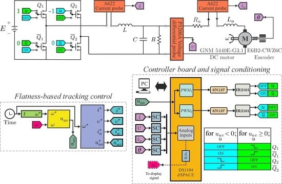
• The subsystem full-bridge Buck inverter, which modulates and feeds with bipolar voltage $\upsilon$ the DC motor through the input u. It is composed of a power supply E and an array of four transistors, denoted as $Q_1$, ${\overline{Q}}_1$, $Q_2$, and ${\overline{Q}}_2$, which operate in accordance with the clock cycles shown in Figure 2. This subsystem is made up of an $LC$ filter, where i is the circulating current over the inductor L, and $\upsilon$ is the voltage appearing across the terminals of the parallel connection between the capacitor C and the load R.
• The subsystem DC motor, which relates to the actuator system and comprises the armature resistance $R_a$, armature inductance $L_a$, and armature current $i_a$. $\omega$ corresponds to the angular velocity associated with the motor shaft. Additional parameters are the moment of inertia of the rotor and motor load J, the viscous friction coefficient of the motor b, the counterelectromotive force constant $k_e$, and the motor torque constant $k_m$.

As stated in [40], the switched model of the full-bridge Buck inverter–DC motor system shown in Figure 2 is given by

$$\begin{array}{cc}\hfill L\frac{di}{dt}& =-\upsilon +Eu,\hfill \\ \hfill C\frac{d\upsilon }{dt}& =i-\frac{\upsilon }{R}-i_a,\hfill \\ \hfill L_a\frac{d{i}_a}{dt}& =\upsilon -R_a{i}_a-k_e\omega ,\hfill \\ \hfill J\frac{d\omega }{dt}& =k_m{i}_a-b\omega ,\hfill \end{array}$$

(1)

where $u\in \{-1,0,1\}$ represents the positions of the transistors $Q_1$, ${\overline{Q}}_1$, $Q_2$, and ${\overline{Q}}_2$ when operating in the negative or positive cycles according to the clock signals u that are shown in Figure 2. The rest of the variables and constants associated with the mathematical model (1) were previously defined. Moreover, according to [40], the average mathematical model of the full-bridge Buck inverter–DC motor system is determined by

$$\begin{array}{cc}\hfill L\frac{di}{dt}& =-\upsilon +E{u}_{av},\hfill \\ \hfill C\frac{d\upsilon }{dt}& =i-\frac{\upsilon }{R}-i_a,\hfill \\ \hfill L_a\frac{d{i}_a}{dt}& =\upsilon -R_a{i}_a-k_e\omega ,\hfill \\ \hfill J\frac{d\omega }{dt}& =k_m{i}_a-b\omega ,\hfill \end{array}$$

(2)

with $u_{av}\in [-1,1]$, where $u_{av}$ is the duty cycle or average input signal of the system. The rest of the variables and constants concerning the mathematical model (2) were previously defined.

3. Robust Flatness-Based Tracking Control

This section presents the development of a robust differential flatness-based tracking control for the full-bridge Buck inverter–DC motor system. Such a control exploits the differential flatness property employed by the mathematical model of system (2). The following proposition summarizes the main result.

Proposition 1. 

Consider the average mathematical model of the full-bridge Buck inverter–DC motor system given in (2), in closed-loop, with the following controller:

$$\begin{array}{cc}{u}_{av}\hfill & =\left[\frac{CJL{L}_a}{k_{m}E}\right]\mu +\left[\frac{bCL{L}_{a}R+CJLR{R}_a+JL{L}_a}{k_{m}RE}\right]{\omega }^{\left(3\right)}\hfill \\ \hfill & +\alpha \ddot{\omega }+\left[\frac{bLR+bL{R}_a+b{L}_{a}R+k_e{k}_{m}L+JR{R}_a}{k_{m}RE}\right]\dot{\omega }+\left[\frac{b{R}_a+k_e{k}_m}{k_{m}E}\right]\omega ,\hfill \end{array}$$

(3)

where

$$\begin{array}{cc}\mu \hfill & ={\omega }^{*\left(4\right)}-k_4\left[{\omega }^{\left(3\right)}-{\omega }^{*\left(3\right)}\right]-k_3\left[\ddot{\omega }-\ddot{{\omega }^{*}}\right]-k_2\left[\dot{\omega }-\dot{{\omega }^{*}}\right]-k_1\left[\omega -{\omega }^{*}\right]\hfill \\ \hfill & -k_0{\int }_0^t\left[\omega -{\omega }^{*}\right]d\tau ,\hfill \end{array}$$

(4)

and

$$\begin{array}{ccc}\hfill k_0& =& a{\omega }_n^4,\hfill \\ \hfill k_1& =& 4a\zeta {\omega }_n^3+{\omega }_n^4,\hfill \\ \hfill k_2& =& 2a{\omega }_n^2+4a{\zeta }^2{\omega }_n^2+4\zeta {\omega }_n^3,\hfill \\ \hfill k_3& =& 4a\zeta {\omega }_n+2{\omega }_n^2+4{\zeta }^2{\omega }_n^2,\hfill \\ \hfill k_4& =& a+4\zeta {\omega }_n.\hfill \end{array}$$

(5)

Then, $\omega \left(t\right)\to {\omega }^{*}\left(t\right)$ exponentially, where ${\omega }^{*}\left(t\right)$ is continuously differentiable up to the fourth time derivative.

Proof. 

In [40], it was demonstrated that the full-bridge Buck inverter–DC motor system average model given in (2) is differentially flat, with the motor angular velocity as the flat output, i.e.,

$$\mathcal{F}=\omega .$$

(6)

This means that all of the state variables x as well as the input $u_{av}$ are given as functions of the flat output and a number of its time derivatives, which is [40]

$$\begin{array}{c}x={\left[\begin{array}{c}i\left(\omega \right),\upsilon \left(\omega \right),i_a\left(\omega \right),\omega \end{array}\right]}^T,u_{av}=u_{av}\left(\omega \right),\end{array}$$

(7)

where

$$\begin{array}{cc}i\left(\omega \right)\hfill & =\left[\frac{CJ{L}_a}{k_m}\right]{\omega }^{\left(3\right)}+\left[\frac{bC{L}_{a}R+CJR{R}_a+J{L}_a}{k_{m}R}\right]\ddot{\omega }\hfill \\ \hfill & +\left[\frac{b{L}_a+JR+J{R}_a+bCR{R}_a+k_e{k}_{m}CR}{k_{m}R}\right]\dot{\omega }+\left[\frac{bR+b{R}_a+k_e{k}_m}{k_{m}R}\right]\omega ,\hfill \end{array}$$

(8)

$$\begin{array}{c}\upsilon \left(\omega \right)=\frac{J{L}_a}{k_m}\ddot{\omega }+\left[\frac{b{L}_a+J{R}_a}{k_m}\right]\dot{\omega }+\left[\frac{b{R}_a}{k_m}+k_e\right]\omega ,\hfill \end{array}$$

(9)

$$\begin{array}{c}{i}_a\left(\omega \right)=\frac{J}{k_m}\dot{\omega }+\frac{b}{k_m}\omega ,\hfill \end{array}$$

(10)

and

$$\begin{array}{cc}{u}_{av}\left(\omega \right)\hfill & =\left[\frac{CJL{L}_a}{k_{m}E}\right]{\omega }^{\left(4\right)}+\left[\frac{bCL{L}_{a}R+CJLR{R}_a+JL{L}_a}{k_{m}RE}\right]{\omega }^{\left(3\right)}+\alpha \ddot{\omega }\hfill \\ \hfill & +\left[\frac{bLR+bL{R}_a+b{L}_{a}R+k_e{k}_{m}L+JR{R}_a}{k_{m}RE}\right]\dot{\omega }+\left[\frac{b{R}_a+k_e{k}_m}{k_{m}E}\right]\omega ,\hfill \end{array}$$

(11)

with

$$\alpha =\frac{bL{L}_a+JLR+JL{R}_a+bCLR{R}_a+k_e{k}_{m}CLR+J{L}_{a}R}{k_{m}RE}.$$

Notice there are four variables that can be known by direct measurements, i.e., $i,\upsilon ,i_a,$ and $\omega$. Moreover, there are three linear Equations (8)–(10). Hence, the three unknowns $\dot{\omega },\ddot{\omega },$ and ${\omega }^{\left(3\right)}$ can be computed. This means that the control law in (3) can be obtained by mimicking (11) and replacing the unknown variable ${\omega }^{\left(4\right)}$ by another variable, say $\mu$. Likewise, notice that (11) represents the flatness-based model of the full-bridge Buck inverter–DC motor system. Thus, (11) and (3) can be equated to obtain the closed-loop dynamics, i.e.,

$${\omega }^{\left(4\right)}=\mu .$$

(12)

This expression represents a linear system given by a chain of four integrators, i.e., an unstable linear system. Hence, $\mu$ must be designed in order to stabilize this chain of integrators. This motivates the definition of $\mu$ in (4) to obtain

$$e^{\left(4\right)}+k_4{e}^{\left(3\right)}+k_3\ddot{e}+k_2\dot{e}+k_{1}e+k_0{\int }_0^{t}e\left(\tau \right)d\tau =0,$$

(13)

where $e\left(t\right)=\omega \left(t\right)-{\omega }^{*}\left(t\right)$. The integral component ensures zero static error in steady state and compensates the abrupt variations that can be generated in some parameters of the system. Differentiating once the above expression with respect to time yields

$$e^{\left(5\right)}+k_4{e}^{\left(4\right)}+k_3{e}^{\left(3\right)}+k_2\ddot{e}+k_1\dot{e}+k_{0}e=0.$$

(14)

This linear fifth-order dynamics is exponentially stable if and only if all of the five roots of the following polynomial have negative real parts

$$P\left(s\right)=s^5+k_4{s}^4+k_3{s}^3+k_2{s}^2+k_{1}s+k_0.$$

(15)

This is ensured if the set of gains $\{k_0,k_1,k_2,k_3,k_4\}$ are chosen such that $P\left(s\right)$ is identical to the following Hurwitz polynomial

$$P_H\left(s\right)=\left(s+a\right){\left(s^2+2\zeta {\omega }_{n}s+{\omega }_n^2\right)}^2,$$

where a, $\zeta$, and ${\omega }_n$ are positive constants. This is accomplished if we choose $\{k_0,k_1,k_2,k_3,k_4\}$ as in (5). Since (14) has been ensured to be exponentially stable, we have that $\omega \left(t\right)\to {\omega }^{*}\left(t\right)$ exponentially.

Now, consider the expressions in (8)–(10), and suppose that $\omega$ is constant, i.e., that all velocity time derivatives are zero. Then, the following is found:

$$\overline{i}\left(\overline{\omega }\right)=\left[\frac{bR+b{R}_a+k_e{k}_m}{k_{m}R}\right]\overline{\omega },$$

(16)

$$\overline{\upsilon }\left(\overline{\omega }\right)=\left[\frac{b{R}_a}{k_m}+k_e\right]\overline{\omega },$$

(17)

$${\overline{i}}_a\left(\overline{\omega }\right)=\frac{b}{k_m}\overline{\omega }.$$

(18)

Assume that uncertainty exists in some of the system parameters appearing in (16)–(18). From these expressions, it can be realized that the steady-state value of the velocity changes if $\overline{i},\overline{\upsilon }$, and ${\overline{i}}_a$, do not change. Hence, consider (13). In order to take into account that the velocity has deviated from its desired steady-state value, we replace $k_{1}e$ by $k_1(\omega +\Delta \omega -{\omega }^{*})$, where $\Delta \omega$ stands for the constant velocity deviation. Then, we obtain

$$e^{\left(4\right)}+k_4{e}^{\left(3\right)}+k_3\ddot{e}+k_2\dot{e}+k_{1}e+k_0{\int }_0^{t}e\left(\tau \right)d\tau =-k_1\Delta \omega .$$

(19)

After differentiating once the above expression, and since $-k_1\Delta \omega$ is a constant, (14) is obtained again. Thus, it is concluded one more time that $\omega \left(t\right)\to {\omega }^{*}\left(t\right)$ exponentially. This completes the proof of Proposition 1. □

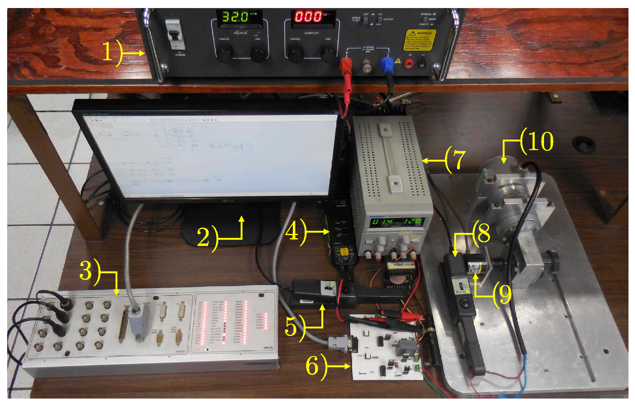
4. Description of the Built Experimental Platform

This section describes the connections of the built prototype full-bridge Buck inverter–DC motor system and the implementation of the designed robust flatness-based control.

A photograph showing the connections of the built full-bridge Buck inverter–DC motor system in closed-loop is exhibited in Figure 3. The elements associated with this photograph are the following: (1) energy power source E, (2) desktop computer, (3) dSPACE DS1104 R&D controller board, (4) voltage differential probe to obtain $\upsilon$ (via a Tektronix P5200A probe), (5) current probe to find i (via a Tektronix A622 probe), (6) full-bridge Buck inverter, (7) energy power source for the instrumentation of the electronics stage, (8) current probe to acquire $i_a$ (via a Tektronix A622 probe), (9) Omron E6B2-CWZ6C encoder to determine $\omega$, and (10) Engel GNM 5440E-G3.1 DC motor.

Figure 4 shows the block diagram of the connections between the system, Simulink, and the dSPACE DS1104 controller board.

The blocks composing the diagram of Figure 4 are as follows:

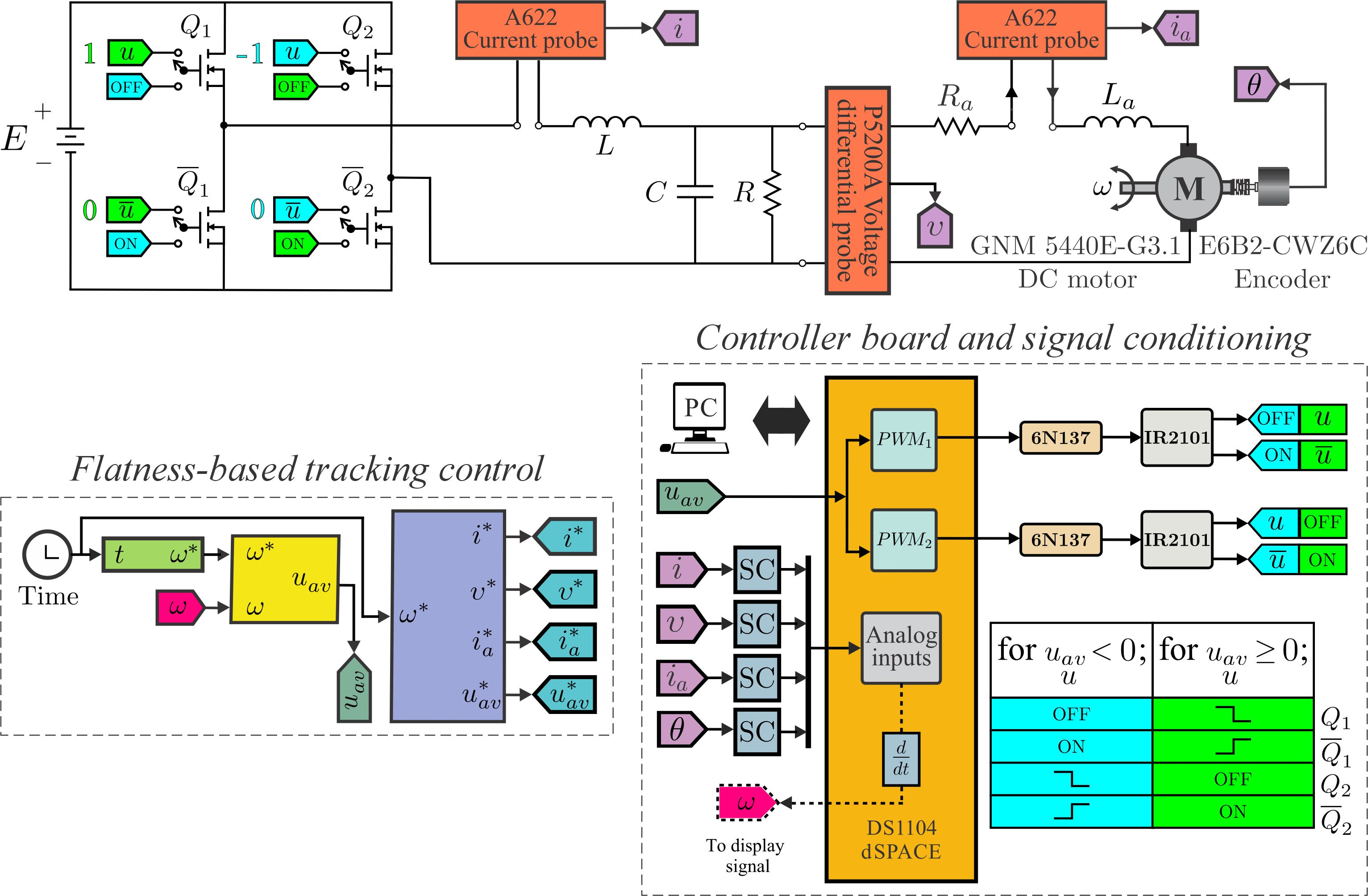
• System. This block corresponds to the built full-bridge Buck inverter–DC motor system. Here, the variables i, $\upsilon$, $i_a$, and $\omega$ were measured via a Tektronix A622 current probe, a Tektronix P5200A voltage probe, a Tektronix A622 current probe, and an Omron E6B2-CWZ6C encoder, respectively. On the other hand, the values of the parameters associated with the Buck converter and the Engel GNM 5440E-G3.1 DC motor were

  $$\begin{array}{c}E=32\mathrm{V},L=4.94\mathrm{mH},C=4.7\mathsf{\mu }\mathrm{F},R=48\mathrm{\Omega },\end{array}$$

  (20)

  and

  $$\begin{array}{c}{L}_a=2.22\mathrm{mH},R_a=0.965\mathrm{\Omega },k_m=120.1\times {10}^{-3}\frac{\mathrm{N}·\mathrm{m}}{\mathrm{A}},\hfill \\ k_e=120.1\times {10}^{-3}\frac{\mathrm{V}·\mathrm{s}}{\mathrm{rad}},J=118.2\times {10}^{-3}\mathrm{kg}·{\mathrm{m}}^2,b=129.6\times {10}^{-3}\frac{\mathrm{N}·\mathrm{m}·\mathrm{s}}{\mathrm{rad}},\hfill \end{array}$$

  (21)

  respectively.
• Flatness-based tracking control. The flatness-based control (3) was implemented in this block with Simulink. On the one hand, the determination of the angular velocity $\omega$, required by the control, was carried out via an E6B2-CWZ6C encoder. On the other hand, the desired angular velocity profile ${\omega }^{*}$, also required by the control, was produced from the desired trajectory subblock. Meanwhile, the control gains were obtained after the parameters $a=0.2$, $\zeta =10$ and ${\omega }_n=1200$ were introduced in (5). Lastly, the reference variables $i^{*}$, ${\upsilon }^{*}$, $i_a^{*}$, and $u_{av}^{*}$ were generated when ${\omega }^{*}$ was replaced into (8)–(10), and (11), respectively.
• Controller board and signal conditioning. In this block, the implementation of the switched control, u, corresponding to the obtained flatness-based tracking control $u_{av}$ (3), was carried out via the PWM subblocks of the dSPACE DS1104 controller board. Thus, after obtaining u, the correct on/off activation of the transistors $Q_1$, ${\overline{Q}}_1$, $Q_2$, and ${\overline{Q}}_2$ of the full-bridge inverter circuit was achieved. Such a circuit was built with four IRF640N MOSFET transistors, two IR2101 drivers, and two 6N137 optocouplers. Finally, the signals i, $\upsilon$, $i_a$, and $\theta$ were correctly adjusted through signal conditioning (SC) blocks.

5. Experimental and Simulation Tests in Closed-Loop and Discussion of the Results

In order to validate the performance of the designed robust flatness-based tracking control, experimental tests were carried out on the aforementioned built experimental platform. After this, by using Matlab–Simulink, the corresponding simulation results were derived, which are presented.

5.1. Results of the System in Closed-Loop

Five different experimental tests were implemented. From the first test to the fourth one, four desired trajectories of ${\omega }^{*}$, along with the system nominal parameters declared in (20) and (21), were considered. In the fifth experimental test, with the aim of verifying the control’s robustness, some perturbations were introduced into the system. In all the plotted graphs, the variables of the system are shown; first $\omega$ and $i_a$ and then i, $\upsilon$, and $u_{av}$. To corroborate the experimental results, the associated simulation results are also shown.

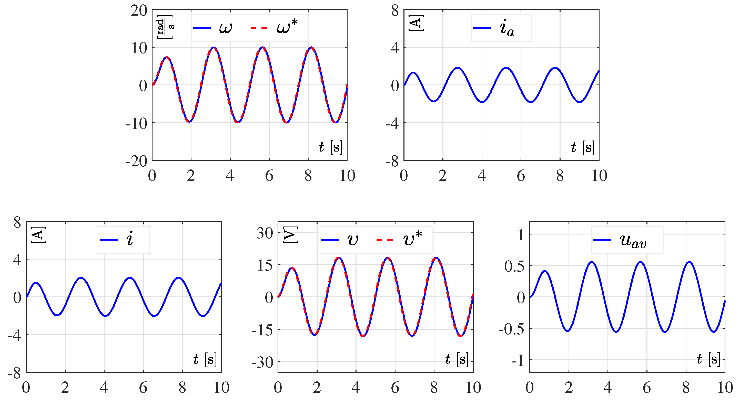
5.1.1. Experimental and Simulation Test 1

In this experiment, the desired angular velocity profile ${\omega }^{*}$ was declared by the tenth-order Bézier polynomial as follows:

$${\omega }^{*}\left(t\right)={\overline{\omega }}_i\left(t_i\right)+[{\overline{\omega }}_f\left(t_f\right)-{\overline{\omega }}_i\left(t_i\right)]\phi \left(t,t_i,t_f\right),$$

(22)

being $\phi \left(t,t_i,t_f\right)$ defined by

$$\phi \left(t,t_i,t_f\right)=\left\{\begin{array}{cc}0\hfill & t\le t_i,\hfill \\ \begin{array}{c}{\left(\frac{t-t_i}{t_f-t_i}\right)}^5\times \left[252-1050\left(\frac{t-t_i}{t_f-t_i}\right)+1800{\left(\frac{t-t_i}{t_f-t_i}\right)}^2\right.\hfill \\ \left.-1575{\left(\frac{t-t_i}{t_f-t_i}\right)}^3+700{\left(\frac{t-t_i}{t_f-t_i}\right)}^4-126{\left(\frac{t-t_i}{t_f-t_i}\right)}^5\right]\hfill \end{array}\hfill & t\in (t_i,t_f),\hfill \\ 1\hfill & t\ge t_f.\hfill \end{array}\right.$$

Here, we proposed ${\overline{\omega }}_i=-10\frac{\mathrm{rad}}{\mathrm{s}}$ and ${\overline{\omega }}_f=10\frac{\mathrm{rad}}{\mathrm{s}}$ for times $t_i=4\mathrm{s}$ and $t_f=6\mathrm{s}$, respectively. Figure 5 shows the experimental evaluation performed by the full-bridge Buck inverter–DC motor system in closed-loop.

The obtained simulation results of this test are shown in Figure 6.

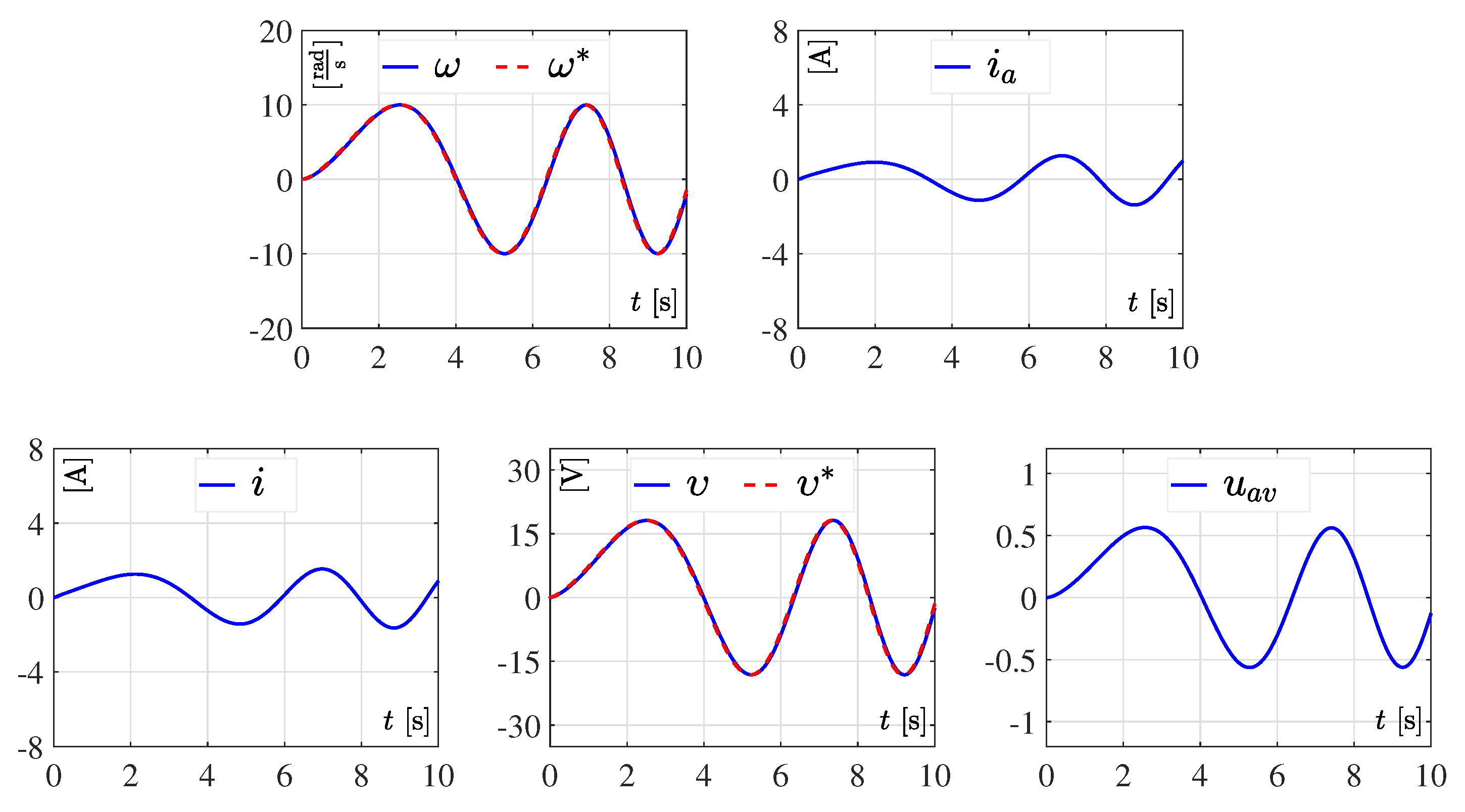
5.1.2. Experimental and Simulation Test 2

To demonstrate the effectiveness of the developed control when periodic signals are contemplated, sinusoidal trajectories were explored as desired angular velocity profiles. Thus, in the second experiment ${\omega }^{*}$ was chosen as:

$${\omega }^{*}\left(t\right)=10\sin \left(0.8\pi t\right).$$

(23)

Figure 7 exhibits the corresponding experimental results of the full-bridge Buck inverter–DC motor system in closed-loop.

The simulation results associated with this desired trajectory are exhibited in Figure 8.

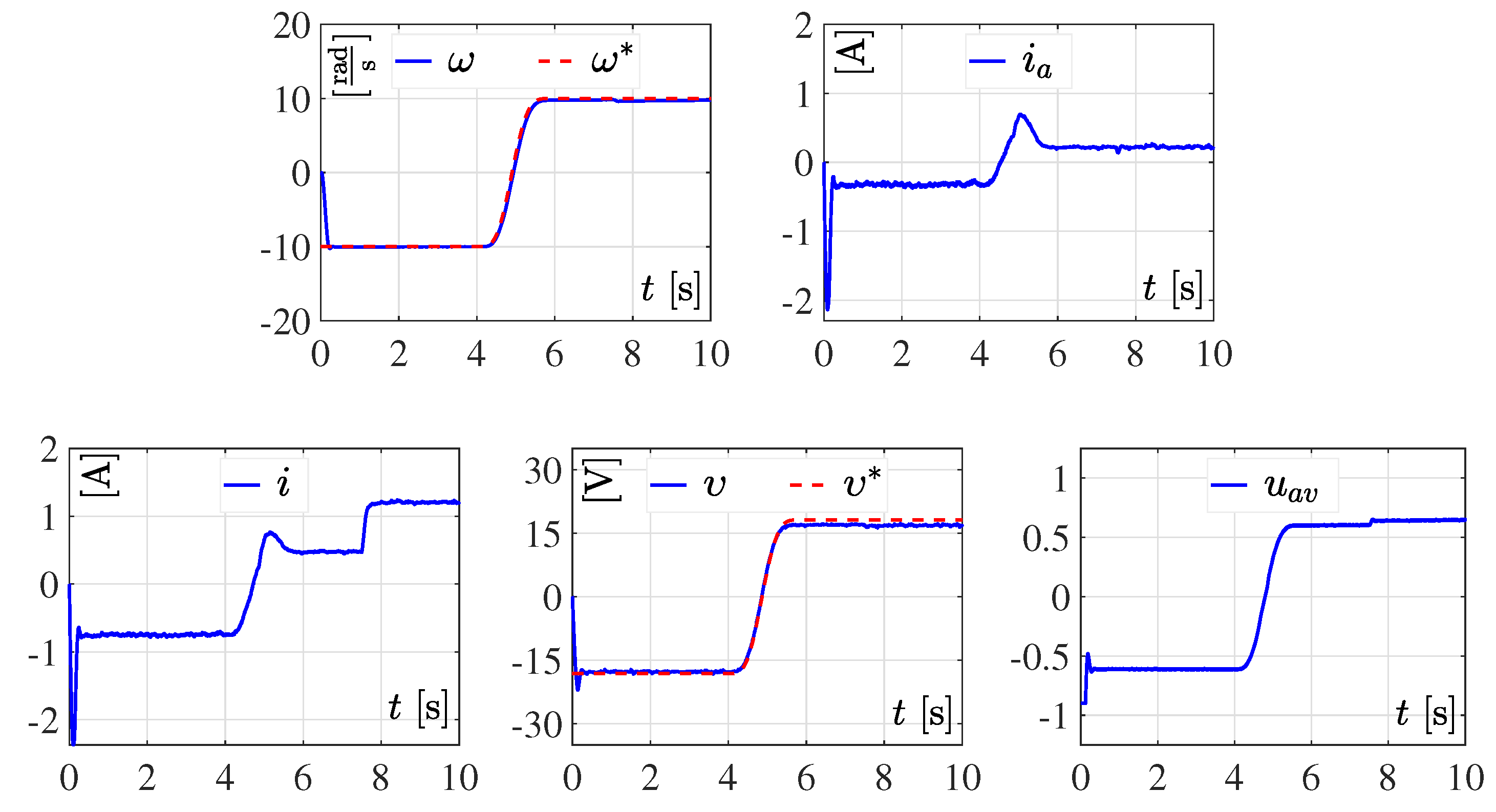
5.1.3. Experimental and Simulation Test 3

A second sinusoidal waveform was considered as the desired trajectory ${\omega }^{*}$ in the implementation of the third experiment. Here, ${\omega }^{*}$ was given by

$${\omega }^{*}\left(t\right)=10\left(1-e^{-2t^2}\right)\sin \left(0.8\pi t\right).$$

(24)

The evolution of the system variables associated with the proposed flatness control approach is illustrated in Figure 9.

The simulation results associated with the experimental results depicted in Figure 9 are presented in Figure 10.

5.1.4. Experimental and Simulation Test 4

In the realization of the fourth experiment, the sinusoidal signal determined by (25) was introduced as the desired trajectory ${\omega }^{*}$, i.e.,

$${\omega }^{*}\left(t\right)=10\sin \left(0.125\pi t^{\frac{3}{2}}\right).$$

(25)

For this experiment, the desired trajectory tracking performance of the system in closed-loop is presented in Figure 11. The corresponding simulation results are shown in Figure 12.

5.1.5. Experimental and Simulation Test 5

Lastly, the fifth experiment was carried out with abrupt perturbations in the converter load R inserted in real time into the built platform of the system. For this experiment, the desired angular velocity profile ${\omega }^{*}$ to be followed by the motor shaft was considered as in (22). Meanwhile, the abrupt perturbations in R were selected as:

$$R_m=\left\{\begin{array}{cc}R\hfill & 0\mathrm{s}\le t<7.5\mathrm{s},\hfill \\ 30\%R\hfill & 7.5\mathrm{s}\le t\le 10\mathrm{s}.\hfill \end{array}\right.$$

(26)

The experimental performance of the flatness-based control when (26) was executed in the system is displayed in Figure 13. The simulation results are displayed in Figure 14.

5.2. Discussion of the Experimental and Simulation Results

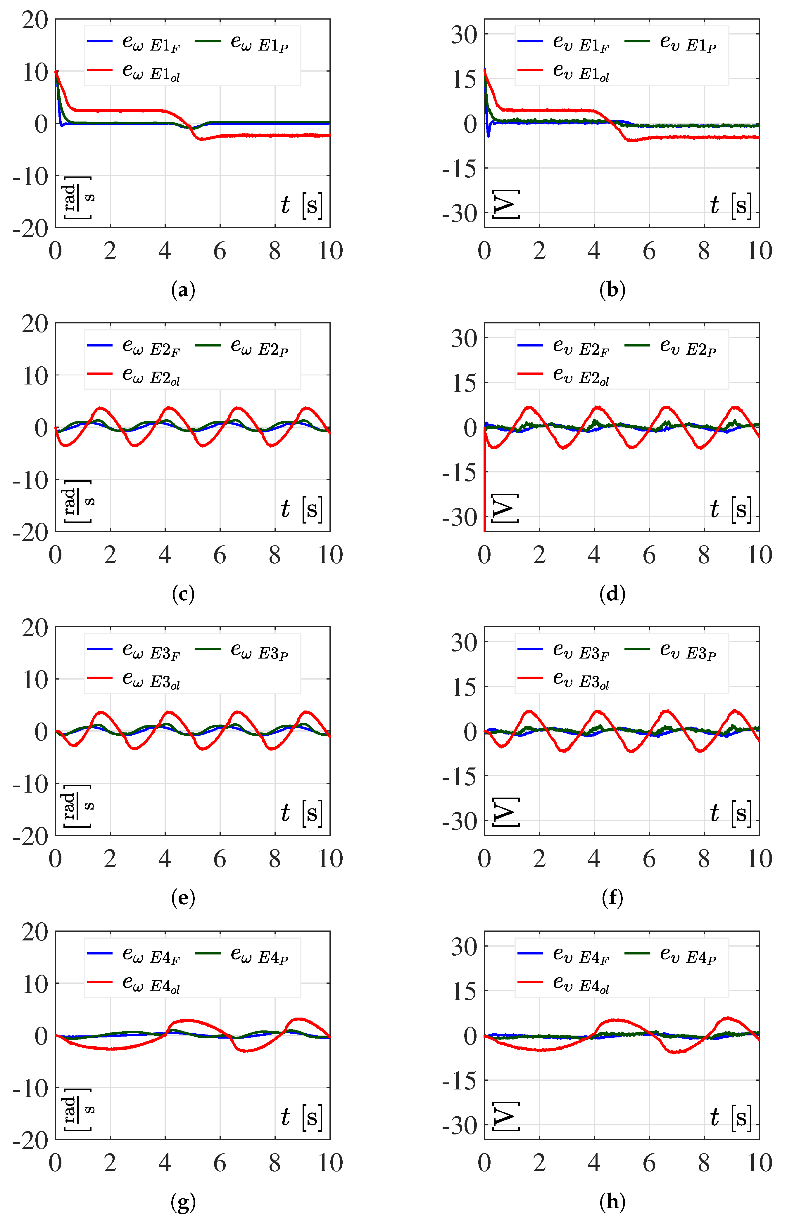
The results of the experimental and simulation tests are discussed here. According to the experimental results presented in Figure 5, Figure 7, Figure 9, Figure 11, and Figure 13 along with the corresponding simulation results depicted in Figure 6, Figure 8, Figure 10, Figure 12, and Figure 14, respectively, we deduced that the flatness-based control satisfactorily accomplished the execution of the angular velocity trajectory tracking task in the full-bridge Buck inverter–DC motor system, i.e., $\omega \to {\omega }^{*}$. Thus, since we have shown that the obtained experimental results and their corresponding simulation results had a similar behavior, the remainder of this section is devoted to the comparative analysis of the experimental results obtained (i.e., by using the flatness concept) with the results reported in the literature.

To highlight the good performance of the designed flatness-based control (3) on the system, in the following, for the four different desired profiles ${\omega }^{*}$, i.e., (22)–(25), the plotted graphics of the tracking errors corresponding to $\omega$ and $\upsilon$ are presented for the next three cases:

1

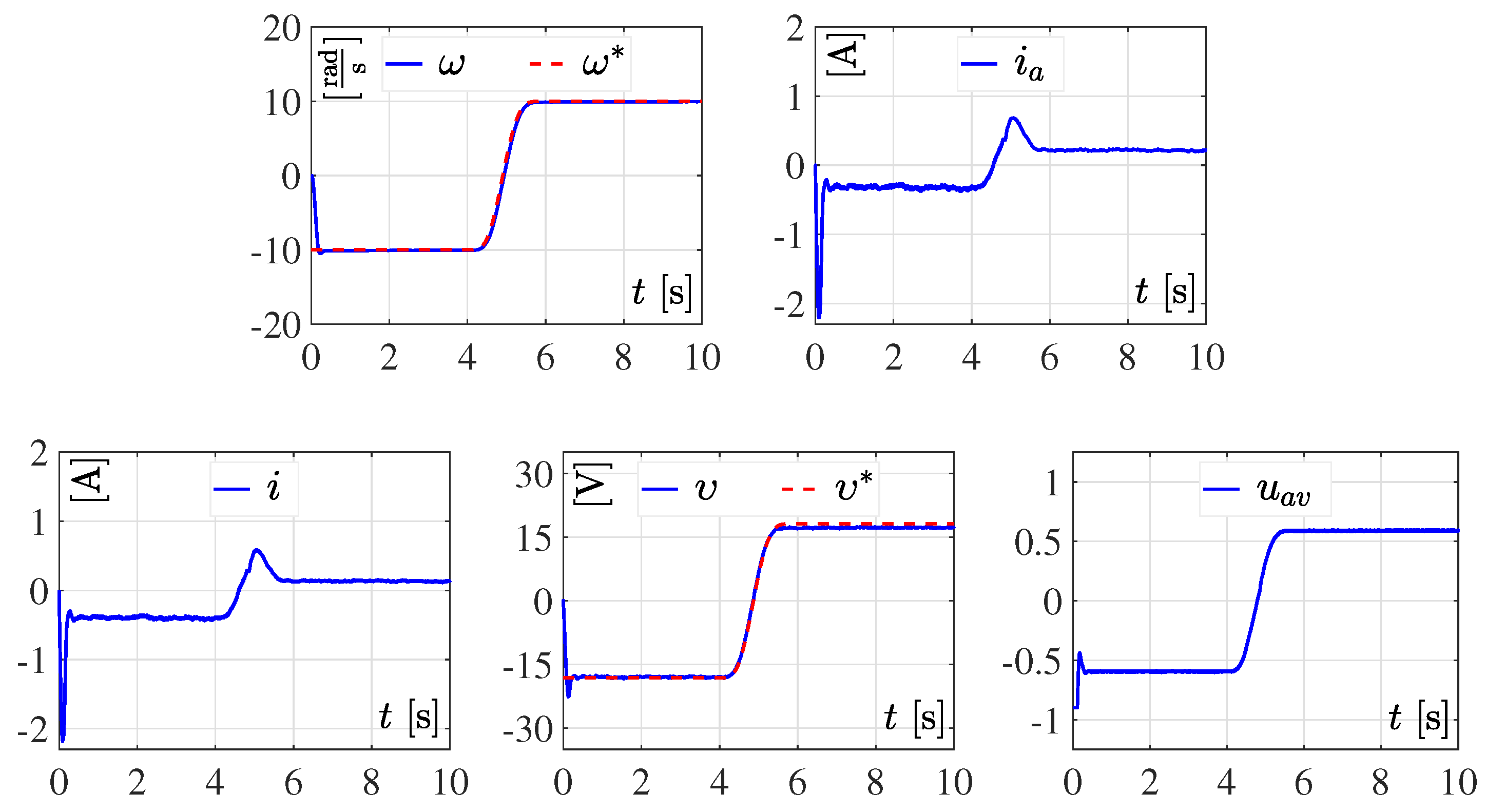
The associated experimental tests of the system in closed-loop with the flatness-based control (studied in this paper). Here, the closed-loop tracking errors for the angular velocity ($e_{\omega E{j}_F}$) and voltage ($e_{\upsilon E{j}_F}$) were determined by

$$\begin{array}{c}\hfill e_{\omega E{j}_F}=\omega -{\omega }^{*},\\ \hfill e_{\upsilon E{j}_F}=\upsilon -{\upsilon }^{*},\end{array}$$

(27)

where subscript $E{j}_F$, for $j\in \{1,2,3,4\}$, associates the experimental test from which the tracking error was obtained. That is, for $j=1$, $j=2$, $j=3$, and $j=4$, the desired trajectories ${\omega }^{*}$ correspond to (22)–(25), respectively.

2

The experimental dynamic responses of the system in closed-loop with the passive control based on the ETEDPOF strategy, developed in [41]. Here, the closed-loop tracking errors of the angular velocity and voltage denoted by $e_{\omega E{j}_P}$ and $e_{\upsilon E{j}_P}$, respectively, were declared as

$$\begin{array}{c}\hfill e_{\omega E{j}_P}=\omega -{\omega }^{*},\\ \hfill e_{\upsilon E{j}_P}=\upsilon -{\upsilon }^{*},\end{array}$$

(28)

where subscript $E{j}_P$, for $j\in \{1,2,3,4\}$, represents the experimental response from which the tracking error was obtained.

3

The obtained experimental results for the system in open-loop, analyzed in [40]. Here, the open-loop tracking errors of the angular velocity ($e_{\omega E{j}_{ol}}$) and voltage ($e_{\upsilon E{j}_{ol}}$) were defined by

$$\begin{array}{c}\hfill e_{\omega E{j}_{ol}}=\omega -{\omega }^{*},\\ \hfill e_{\upsilon E{j}_{ol}}=\upsilon -{\upsilon }^{*},\end{array}$$

(29)

where subscript $E{j}_{ol}$, for $j\in \{1,2,3,4\}$, indicates the experimental result in open-loop from which the tracking error was obtained.

Figure 15 depicts the plotted graphics of the tracking errors related to $\omega$ and $\upsilon$ given by (27)–(29) of the full-bridge Buck inverter–DC motor system. On the one hand, according to Figure 15a,c,e,g, it can be seen that the closed-loop tracking errors obtained with the flatness-based control for $\omega$ (i.e., $e_{\omega E{\{1,2,3,4\}}_F}$) were lower in magnitude than the closed-loop tracking errors associated with the passive control (i.e., $e_{\omega E{\{1,2,3,4\}}_P}$). In addition, in accordance with Figure 15b,d,f,h, a similar evaluation was achieved for the flatness closed-loop tracking errors corresponding to $\upsilon$ (i.e., $e_{\upsilon E{\{1,2,3,4\}}_F}$) in comparison with their associated passive closed-loop tracking errors (i.e., $e_{\upsilon E{\{1,2,3,4\}}_P}$). Meanwhile, note that the open-loop tracking errors, defined in (29) for $\omega$ and $\upsilon$ (i.e., $e_{\omega E{\{1,2,3,4\}}_{ol}}$ and $e_{\upsilon E{\{1,2,3,4\}}_{ol}}$), are also presented in Figure 15 with the aim of exhibiting how the system profited from the proposed flatness-based control and the developed passive control reported in [41] and not for the purpose of comparative evaluation. On the other hand, a visual comparison between the experimental results of the passivity-based control reported in [41] (see Figure 1) and the experimental results of the designed flatness-based control (see Figure 13) shows how the performance of the latter control was superior. This is due to the fact that it is robust against parametric variations in comparison with the passivity-based control.

Lastly, from the aforementioned comments on the experimental results, it is inferred that the developed flatness-based control given by (3) satisfactorily carried out the aim of solving the angular velocity trajectory tracking problem in the full-bridge Buck inverter–DC motor system, that is, $\omega \to {\omega }^{*}$.

6. Conclusions

A robust differential flatness-based control for carrying out the angular velocity trajectory tracking task associated with the full-bridge Buck inverter–DC motor system was developed and experimentally validated in this work. This robust control was designed by exploiting the differential flatness property of the mathematical model related to the full-bridge Buck inverter–DC motor system. Then, the experimental implementation of the robust flatness-based control was programmed by utilizing Simulink and a dSPACE DS1104 controller board on a built prototype of the full-bridge Buck inverter–DC motor system. Lastly, the closed-loop system was also programmed in Matlab–Simulink with the purpose of obtaining the corresponding simulation results. After analyzing the experimental results of the closed-loop system, it was concluded that the control objective, i.e., $\omega \to {\omega }^{*}$, was solved even when abrupt variations were added to the nominal parameters of the system. Such a conclusion was corroborated by comparison with the simulation results.

Finally, derived from the experimental results satisfactorily obtained, future work could be developed on proposing this system as a viable electronics power stage for AC motors, renewable energy systems, electromechanical systems, robotic arms, wheeled mobile robots, uncrewed underwater vehicles, and mechatronic systems.

References

1. Gieras, J.F. Permanent Magnet Motor Technology: Design and Applications, 3rd ed.; CRC Press: New York, NY, USA, 2010. [Google Scholar]
2. Lyshevski, S.E. Electromechanical Systems, Electric Machines, and Applied Mechatronics; CRC Press: Boca Raton, FL, USA, 2000; ISBN 0-8493-2275-8. [Google Scholar]
3. Ahmad, M.A.; Ismail, R.M.T.R.; Ramli, M.S. Control strategy of Buck converter driven DC motor: A comparative assessment. Austral. J. Basic Appl. Sci. 2010, 4, 4893–4903. [Google Scholar]
4. Bingöl, O.; Paçaci, S. A virtual laboratory for neural network controlled DC motors based on a DC-DC Buck converter. Int. J. Eng. Educ. 2012, 28, 713–723. [Google Scholar]
5. Sira-Ramírez, H.; Oliver-Salazar, M.A. On the robust control of Buck-converter DC-motor combinations. IEEE Trans. Power Electron. 2013, 28, 3912–3922. [Google Scholar] [CrossRef]
6. Yang, J.; Wu, H.; Hu, L.; Li, S. Robust predictive speed regulation of converter-driven DC motors via a discrete-time reduced-order GPIO. IEEE Trans. Ind. Electron. 2019, 66, 7893–7903. [Google Scholar] [CrossRef] [Green Version]
7. Stanković, M.R.; Madonski, R.; Shao, S.; Mikluc, D. On dealing with harmonic uncertainties in the class of active disturbance rejection controllers. Int. J. Control 2021, 94, 2795–2810. [Google Scholar] [CrossRef]
8. Madonski, R.; Łakomy, K.; Stankovic, M.; Shao, S.; Yang, J.; Li, S. Robust converter-fed motor control based on active rejection of multiple disturbances. Control Eng. Pract. 2021, 107, 104696. [Google Scholar] [CrossRef]
9. Zhang, L.; Yang, J.; Li, S. A model-based unmatched disturbance rejection control approach for speed regulation of a converter-driven DC motor using output-feedback. IEEE-CAA J. Autom. Sin. 2022, 9, 365–376. [Google Scholar] [CrossRef]
10. Guerrero-Ramírez, E.; Martínez-Barbosa, A.; Guzmán-Ramírez, E.; Barahona-Ávalos, J.L. Design methodology for digital active disturbance rejection control of the DC motor drive. e-Prime—Adv. Electr. Eng. Electron. Energy 2022, 2, 100050. [Google Scholar] [CrossRef]
11. Guerrero-Ramírez, E.; Martínez-Barbosa, A.; Contreras-Ordaz, M.A.; Guerrero-Ramírez, G.; Guzman-Ramirez, E.; Barahona-Ávalos, J.L.; Adam-Medina, M. DC motor drive powered by solar photovoltaic energy: An FPGA-based active disturbance rejection control approach. Energies 2022, 15, 6595. [Google Scholar] [CrossRef]
12. Rigatos, G.; Siano, P.; Wira, P.; Sayed-Mouchaweh, M. Control of DC–DC converter and DC motor dynamics using differential flatness theory. Intell. Ind. Syst. 2016, 2, 371–380. [Google Scholar] [CrossRef] [Green Version]
13. Rigatos, G.; Siano, P.; Ademi, S.; Wira, P. Flatness-based control of DC-DC converters implemented in successive loops. Electr. Power Compon. Syst. 2018, 46, 673–687. [Google Scholar] [CrossRef]
14. Silva-Ortigoza, R.; Roldán-Caballero, A.; Hernández-Márquez, E.; García-Sánchez, J.R.; Marciano-Melchor, M.; Hernández-Guzmán, V.M.; Silva-Ortigoza, G. Robust flatness tracking control for the “DC/DC Buck converter-DC motor” system: Renewable energy-based power supply. Complexity 2021, 2021, 2158782. [Google Scholar] [CrossRef]
15. Hoyos, F.E.; Rincón, A.; Taborda, J.A.; Toro, N.; Angulo, F. Adaptive quasi-sliding mode control for permanent magnet DC motor. Math. Probl. Eng. 2013, 2013, 693685. [Google Scholar] [CrossRef] [Green Version]
16. Hoyos Velasco, F.E.; Candelo-Becerra, J.E.; Rincón Santamaria, A. Dynamic analysis of a permanent magnet DC motor using a Buck converter controlled by ZAD-FPIC. Energies 2018, 11, 3388. [Google Scholar] [CrossRef] [Green Version]
17. Hoyos, F.E.; Candelo-Becerra, J.E.; Hoyos Velasco, C.I. Application of zero average dynamics and fixed point induction control techniques to control the speed of a DC motor with a Buck converter. Appl. Sci. 2020, 10, 1807. [Google Scholar] [CrossRef] [Green Version]
18. Hoyos, F.E.; Candelo-Becerra, J.E.; Rincón, A. Zero average dynamic controller for speed control of DC motor. Appl. Sci. 2021, 11, 5608. [Google Scholar] [CrossRef]
19. Wei, F.; Yang, P.; Li, W. Robust adaptive control of DC motor system fed by Buck converter. Int. J. Control Autom. 2014, 7, 179–190. [Google Scholar] [CrossRef]
20. Silva-Ortigoza, R.; Hernández-Guzmán, V.M.; Antonio-Cruz, M.; Muñoz-Carrillo, D. DC/DC Buck power converter as a smooth starter for a DC motor based on a hierarchical control. IEEE Trans. Power Electron. 2015, 30, 1076–1084. [Google Scholar] [CrossRef]
21. Hernández-Guzmán, V.M.; Silva-Ortigoza, R.; Muñoz-Carrillo, D. Velocity control of a brushed DC-motor driven by a DC to DC Buck power converter. Int. J. Innov. Comp. Inf. Control 2015, 11, 509–521. [Google Scholar] [CrossRef]
22. Rauf, A.; Li, S.; Madonski, R.; Yang, J. Continuous dynamic sliding mode control of converter-fed DC motor system with high order mismatched disturbance compensation. Trans. Inst. Meas. Control 2020, 42, 2812–2821. [Google Scholar] [CrossRef]
23. Rauf, A.; Zafran, M.; Khan, A.; Tariq, A.R. Finite-time nonsingular terminal sliding mode control of converter-driven DC motor system subject to unmatched disturbances. Int. Trans. Elect. Energy Syst. 2021, 31, e13070. [Google Scholar] [CrossRef]
24. Ravikumar, D.; Srinivasan, G.K. Implementation of higher order sliding mode control of DC–DC Buck converter fed permanent magnet DC motor with improved performance. Automatika 2022. [Google Scholar] [CrossRef]
25. Khubalkar, S.; Chopade, A.; Junghare, A.; Aware, M.; Das, S. Design and realization of stand-alone digital fractional order PID controller for Buck converter fed DC motor. Circuits Syst. Signal Process. 2016, 35, 2189–2211. [Google Scholar] [CrossRef]
26. Khubalkar, S.W.; Junghare, A.S.; Aware, M.V.; Chopade, A.S.; Das, S. Demonstrative fractional order—PID controller based DC motor drive on digital platform. ISA Trans. 2018, 82, 79–93. [Google Scholar] [CrossRef] [PubMed]
27. Patil, M.D.; Vadirajacharya, K.; Khubalkar, S.W. Design and tuning of digital fractional-order PID controller for permanent magnet DC motor. IETE J. Res. 2021. [Google Scholar] [CrossRef]
28. Kumar, S.G.; Thilagar, S.H. Sensorless load torque estimation and passivity based control of Buck converter fed DC motor. Sci. World J. 2015, 2015, 132843. [Google Scholar] [CrossRef] [Green Version]
29. Srinivasan, G.K.; Srinivasan, H.T.; Rivera, M. Sensitivity Analysis of Exact Tracking Error Dynamics Passive Output Control for a Flat/Partially Flat Converter Systems. Electronics 2020, 9, 1942. [Google Scholar] [CrossRef]
30. Nizami, T.K.; Chakravarty, A.; Mahanta, C. Design and implementation of a neuro-adaptive backstepping controller for Buck converter fed PMDC-motor. Control Eng. Pract. 2017, 58, 78–87. [Google Scholar] [CrossRef]
31. Nizami, T.K.; Chakravarty, A.; Mahanta, C.; Iqbal, A.; Hosseinpour, A. Enhanced dynamic performance in DC–DC converter-PMDC motor combination through an intelligent non-linear adaptive control scheme. IET Power Electron. 2022. [Google Scholar] [CrossRef]
32. Nizami, T.K.; Gangula, S.D.; Reddy, R.; Dhiman, H.S. Legendre neural network based intelligent control of DC-DC step down converter-PMDC motor combination. IFAC 2022, 55, 162–167. [Google Scholar] [CrossRef]
33. Hanif, M.I.F.M.; Suid, M.H.; Ahmad, M.A. A piecewise affine PI controller for Buck converter generated DC motor. Int. J. Power Electron. Drive Syst. 2019, 10, 1419–1426. [Google Scholar] [CrossRef]
34. Rigatos, G.; Siano, P.; Sayed-Mouchaweh, M. Adaptive neurofuzzy H-infinity control of DC-DC voltage converters. Neural Comput. Appl. 2020, 33, 2507–2520. [Google Scholar] [CrossRef]
35. Kazemi, M.G.; Montazeri, M. Fault detection of continuous time linear switched systems using combination of bond graph method and switching observer. ISA Trans. 2019, 94, 338–351. [Google Scholar] [CrossRef] [PubMed]
36. Silva-Ortigoza, R.; Alba-Juárez, J.N.; García-Sánchez, J.R.; Antonio-Cruz, M.; Hernández-Guzmán, V.M.; Taud, H. Modeling and experimental validation of a bidirectional DC/DC Buck power electronic converter–DC motor system. IEEE Latin Am. Trans. 2017, 15, 1043–1051. [Google Scholar] [CrossRef]
37. Silva-Ortigoza, R.; Alba-Juárez, J.N.; García-Sánchez, J.R.; Hernández-Guzmán, V.M.; Sosa-Cervantes, C.Y.; Taud, H. A sensorless passivity-based control for the DC/DC Buck converter–Inverter–DC motor system. IEEE Latin Am. Trans. 2016, 14, 4227–4234. [Google Scholar] [CrossRef]
38. Hernández-Márquez, E.; García-Sánchez, J.R.; Silva-Ortigoza, R.; Antonio-Cruz, M.; Hernández-Guzmán, V.M.; Taud, H.; Marcelino-Aranda, M. Bidirectional tracking robust controls for a DC/DC Buck converter-DC motor system. Complexity 2018, 2018, 1260743. [Google Scholar] [CrossRef]
39. Chi, X.; Quan, S.; Chen, J.; Wang, Y.-X.; He, H. Proton exchange membrane fuel cell-powered bidirectional DC motor control based on adaptive sliding-mode technique with neural network estimation. Int. J. Hydrog. Energy 2020, 45, 20282–20292. [Google Scholar] [CrossRef]
40. Hernández-Márquez, E.; Avila-Rea, C.A.; García-Sánchez, J.R.; Silva-Ortigoza, R.; Marciano-Melchor, M.; Marcelino-Aranda, M.; Roldán-Caballero, A.; Márquez-Sánchez, C. New “full-bridge Buck inverter—DC motor” system: Steady-state and dynamic analysis and experimental validation. Electronics 2019, 8, 1216. [Google Scholar] [CrossRef] [Green Version]
41. Silva-Ortigoza, R.; Hernandez-Marquez, E.; Roldan-Caballero, A.; Tavera-Mosqueda, S.; Marciano-Melchor, M.; Garcia-Sanchez, J.R.; Hernandez-Guzman, V.M.; Silvia-Ortigoza, R. Sensorless tracking control for a “full-bridge Buck inverter—DC motor” system: Passivity and flatness-based design. IEEE Access 2021, 9, 132191–132204. [Google Scholar] [CrossRef]
42. Linares-Flores, J.; Reger, J.; Sira-Ramírez, H. Load torque estimation and passivity-based control of a Boost-converter/DC-motor combination. IEEE Trans. Control Syst. Technol. 2010, 18, 1398–1405. [Google Scholar] [CrossRef]
43. Alexandridis, A.T.; Konstantopoulos, G.C. Modified PI speed controllers for series-excited DC motors fed by DC/DC Boost converters. Control Eng. Pract. 2014, 23, 14–21. [Google Scholar] [CrossRef]
44. Malek, S. A new nonlinear controller for DC-DC Boost converter fed DC motor. Int. J. Power Electron. 2015, 7, 54–71. [Google Scholar] [CrossRef]
45. Konstantopoulos, G.C.; Alexandridis, A.T. Enhanced control design of simple DC-DC Boost converter-driven DC motors: Analysis and implementation. Electr. Power Compon. Syst. 2015, 43, 1946–1957. [Google Scholar] [CrossRef]
46. Mishra, P.; Banerjee, A.; Ghosh, M.; Baladhandautham, C.B. Digital pulse width modulation sampling effect embodied steady-state time-domain modeling of a Boost converter driven permanent magnet DC brushed motor. Int. Trans. Elect. Energy Syst. 2021, 31, e12970. [Google Scholar] [CrossRef]
47. Govindharaj, A.; Mariappan, A. Design and analysis of novel Chebyshev neural adaptive backstepping controller for Boost converter fed PMDC motor. Int. J. Autom. Control 2020, 14, 694–712. [Google Scholar] [CrossRef]
48. Alajmi, B.; Ahmed, N.A.; Al-Othman, A.K. Small-signal analysis and hardware implementation of Boost converter fed PMDC motor for electric vehicle applications. J. Eng. Res. 2021, 9, 189–208. [Google Scholar] [CrossRef]
49. Manikandan, C.T.; Sundarrajan, G.T.; Krishnan, V.G.; Ofori, I. Performance analysis of two-loop interleaved Boost converter fed PMDC-motor system using FLC. Math. Probl. Eng. 2022, 2022, 1639262. [Google Scholar] [CrossRef]
50. García-Sánchez, J.R.; Hernández-Márquez, E.; Ramírez-Morales, J.; Marciano-Melchor, M.; Marcelino-Aranda, M.; Taud, H.; Silva-Ortigoza, R. A robust differential flatness-based tracking control for the “MIMO DC/DC Boost converter—Inverter—DC motor” system: Experimental results. IEEE Access 2019, 7, 84497–84505. [Google Scholar] [CrossRef]
51. Egidio, L.N.; Deacto, G.S.; Jungers, R.M. Stabilization of rank-deficient continuous-time switched affine systems. Automatica 2022, 143, 110426. [Google Scholar] [CrossRef]
52. Sönmez, Y.; Dursun, M.; Güvenç, U.; Yilmaz, C. Start up current control of Buck-Boost convertor-fed serial DC motor. Pamukkale Univ. J. Eng. Sci. 2009, 15, 278–283. [Google Scholar]
53. Linares-Flores, J.; Barahona-Avalos, J.L.; Sira-Ramírez, H.; Contreras-Ordaz, M.A. Robust passivity-based control of a Buck–Boost-converter/DC-motor system: An active disturbance rejection approach. IEEE Trans. Ind. Appl. 2012, 48, 2362–2371. [Google Scholar] [CrossRef]
54. Hernández-Márquez, E.; Avila-Rea, C.A.; García-Sánchez, J.R.; Silva-Ortigoza, R.; Silva-Ortigoza, G.; Taud, H.; Marcelino-Aranda, M. Robust tracking controller for a DC/DC Buck-Boost converter–Inverter–DC motor system. Energies 2018, 11, 2500. [Google Scholar] [CrossRef] [Green Version]
55. Ghazali, M.R.; Ahmad, M.A.; Ismail, R.M.T.R. Adaptive safe experimentation dynamics for data-driven neuroendocrine-PID control of MIMO systems. IETE J. Res. 2022, 68, 1611–1624. [Google Scholar] [CrossRef]
56. Linares-Flores, J.; Sira-Ramírez, H.; Cuevas-López, E.F.; Contreras-Ordaz, M.A. Sensorless passivity based control of a DC motor via a solar powered Sepic converter-full bridge combination. J. Power Electron. 2011, 11, 743–750. [Google Scholar] [CrossRef] [Green Version]
57. Srinivasan, G.K.; Srinivasan, H.T.; Rivera, M. Low-cost implementation of passivity-based control and estimation of load torque for a Luo converter with dynamic load. Electronics 2020, 9, 1914. [Google Scholar] [CrossRef]
58. Arshad, M.H.; Abido, M.A. Hierarchical control of DC motor coupled with Cuk converter combining differential flatness and sliding mode control. Arab. J. Sci. Eng. 2021, 46, 9413–9422. [Google Scholar] [CrossRef]
59. Ismail, A.A.A.; Elnady, A. Advanced drive system for DC motor using multilevel DC/DC Buck converter circuit. IEEE Access 2019, 7, 54167–54178. [Google Scholar] [CrossRef]
60. Guerrero, E.; Guzmán, E.; Linares, J.; Martínez, A.; Guerrero, G. FPGA-based active disturbance rejection velocity control for a parallel DC/DC Buck converter-DC motor system. IET Power Electron. 2020, 13, 356–367. [Google Scholar] [CrossRef]
61. Erenturk, K. Hybrid control of a mechatronic system: Fuzzy logic and grey system modeling approach. IEEE/ASME Trans. Mechatron 2007, 12, 703–710. [Google Scholar] [CrossRef]
62. Swathi, K.V.R.; Nagesh-Kumar, G.V. Design of intelligent controller for reduction of chattering phenomenon in robotic arm: A rapid prototyping. Comput. Electr. Eng. 2019, 74, 483–497. [Google Scholar] [CrossRef]
63. García-Sánchez, J.R.; Tavera-Mosqueda, S.; Silva-Ortigoza, R.; Hernández-Guzmán, V.M.; Marciano-Melchor, M.; Rubio, J.J.; Ponce-Silva, M.; Hernández-Bolaños, M.; Martínez-Martínez, J. A novel dynamic three-level tracking controller for mobile robots considering actuators and power stage subsystems: Experimental assessment. Sensors 2020, 20, 4959. [Google Scholar] [CrossRef] [PubMed]
64. Hernández-Guzmán, V.M.; Silva-Ortigoza, R.; Tavera-Mosqueda, S.; Marcelino-Aranda, M.; Marciano-Melchor, M. Path-tracking of a WMR fed by inverter-DC/DC Buck power electronic converter systems. Sensors 2020, 20, 6522. [Google Scholar] [CrossRef] [PubMed]
65. Zhao, Z.; Yang, J.; Li, S.; Yu, X.; Wang, Z. Continuous output feedback TSM control for uncertain systems with a DC-AC inverter example. IEEE Trans. Circuit Syst. II Express Briefs 2018, 65, 71–75. [Google Scholar] [CrossRef]
66. Chang, E.-C.; Cheng, C.-A.; Wu, R.-C. Robust optimal tracking control of a full-bridge DC-AC converter. Appl. Sci. 2021, 11, 1211. [Google Scholar] [CrossRef]
Figure 1. Experimental results of the passivity-based control reported in [41], when ω * is of the Bézier type (22), and the abrupt variations in load R, declared in (26), are carried out in the system.
Mathematics 10 04110 g001
Figure 2. Full-bridge Buck inverter–DC motor system and clock signals u associated with Q 1 , Q ¯ 1 , Q 2 , and Q ¯ 2 , for the negative duty cycle ( u a v < 0 ) and for the positive duty cycle ( u a v 0 ) .
Mathematics 10 04110 g002
Figure 3. Photograph of the hardware used for the experimental tests of the full-bridge Buck inverter–DC motor system in closed-loop.
Mathematics 10 04110 g003
Figure 4. Connections between the software and hardware blocks of the built full-bridge Buck inverter–DC motor system in closed-loop.
Mathematics 10 04110 g004
Figure 5. Experimental dynamic response of the full-bridge Buck inverter–DC motor system in closed-loop for the first desired trajectory ω * (22).
Mathematics 10 04110 g005
Figure 6. Simulation results of the full-bridge Buck inverter–DC motor system in closed-loop for the first desired trajectory ω * (22).
Mathematics 10 04110 g006
Figure 7. Experimental results when the second desired angular velocity profile, given by (23), is contemplated for the system in closed-loop.
Mathematics 10 04110 g007
Figure 8. Simulation results when the second desired angular velocity profile, given by (23), is contemplated for the system in closed-loop.
Mathematics 10 04110 g008
Figure 9. Experimental response of the system in closed-loop for the third desired angular velocity ω * (24).
Mathematics 10 04110 g009
Figure 10. Simulation response of the system in closed-loop for the third desired angular velocity ω * (24).
Mathematics 10 04110 g010
Figure 11. Experimental results of the system in closed-loop, when the fourth desired trajectory for ω * , determined by (25), is taken into account.
Mathematics 10 04110 g011
Figure 12. Simulation results of the system in closed-loop when the fourth desired trajectory for ω * , determined by (25), is taken into account.
Mathematics 10 04110 g012
Figure 13. Experimental results associated with the designed flatness-based control (3), when ω * is of the Bézier type (22), and the abrupt variations in load R, declared in (26), are introduced into the system.
Mathematics 10 04110 g013
Figure 14. Simulation results associated with the designed flatness-based control (3), when ω * is of the Bézier type (22), and the abrupt variations in load R, declared in (26), are introduced into the system.
Mathematics 10 04110 g014
Figure 15. Plotted graphics of the tracking errors associated with variables ω and υ of the full-bridge Buck inverter–DC motor system. The signal pairs e ω E { 1 , 2 , 3 , 4 } F e υ E { 1 , 2 , 3 , 4 } F , e ω E { 1 , 2 , 3 , 4 } P e υ E { 1 , 2 , 3 , 4 } P , and e ω E { 1 , 2 , 3 , 4 } o l e υ E { 1 , 2 , 3 , 4 } o l are the tracking errors obtained for ω and υ , when the system considers the flatness-based control, the passivity-based control [41], and the experimental results in open-loop [40], respectively. (a) Tracking errors of ω , for the desired trajectory ω * declared in (22). (b) Tracking errors of υ , for the desired trajectory ω * declared in (22). (c) Tracking errors of ω , when the desired profile ω * is given by (23). (d) Tracking errors of υ , when the desired profile ω * is given by (23). (e) Tracking errors of ω , for ω * defined by (24). (f) Tracking errors of υ , for ω * defined by (24). (g) Tracking errors of ω , for the desired trajectory considered in (25). (h) Tracking errors of υ , for the desired trajectory considered in (25).
Mathematics 10 04110 g015
Publisher’s Note: MDPI stays neutral with regard to jurisdictional claims in published maps and institutional affiliations.