1. Introduction
In a survival analysis, the frailty model is a popular approach to model time to event data, which considers both observable and unobservable factors simultaneously [
1]. A large number of studies have demonstrated that the consideration of unobservable variability improves the fitness of the model [
2,
3,
4,
5]. In the frailty model there is an assumption on the explanatory variables that the variable are independent to each other, while various practical situations do not satisfy this assumption. Several studies of infant survival considered factors such as place of residence, birth order, breastfeeding, mother education, tetanus toxoid, antenatal care, iron folic acid tablets, place of delivery, etc. [
6,
7,
8,
9]. Some of the variables, for example tetanus toxoid and antenatal care, are correlated to each other in the data set, which is analyzed in this study. The fact that parameter estimates become unstable when the explanatory variables are correlated in the case of the frailty model, means that the collinearity problem has seldom been considered.
To overcome the problem of collinearity ridge estimation is the alternative of the maximum likelihood estimation. Ridge estimator has smaller MSE than MLE. In the case of high multicollinearity, there is a considerable reduction in MSE. Ridge regression was originally proposed by Hoerl and Kennard (1970a,b) [
10,
11], and later on Schafer et al. (1984) [
12] generalized this approach to logistic regression. A slightly different approach in the connection of the ridge type estimator is given by Daffy and Santner (1989) [
13]. This approach is proposed in a standard linear regression, while Cessie and Houwelingen (1992) [
14] generalized the same approach in logistic regression. However, this method is not adapted for frailty models.
This study developed a ridge regression estimator in the parametric frailty model and evaluated its performance through a simulation study. Further, the proposed approach is applied to examine the risk of infant mortality in India.
2. Ridge Estimator for Parametric Frailty Model
In this section, the approach of Cessie and Houwelingen (1992) [
14] is extended to the parametric frailty model. The ridge estimator is derived as a restricted maximum likelihood estimator.
Frailty model is a mixture model in the survival analysis, where the risk of the individual death (hazard function) is a function of observable factors and a random effect term (unobserved frailty) [
1,
15]. The form of such a model is given as
where
is the hazard of
i-th individual at time
with covariate vector
and unobserved frailty variable
.
is the base line hazard function and
is the vector of regression coefficients. Here,
q represent the number of regressors. It is assumed that the unobserved frailty follow a gamma distribution and is captured by its variance
[
16,
17]. This paper also assumes that the unobserved frailty follows gamma distribution. One assumption is also added on the response variable that it follows Weibull distribution with one parameter
. On the basis of this assumption,
. The likelihood function of the frailty model (1) is given by,
Using the assumption of the distribution (i.e., gamma distribution) of frailty, the random terms are resulted out, making the likelihood function,
The log likelihood form of (3) is
The maximization of (4) gives the ordinary MLE
for
. Since (4) is non linear in
,
m-th, the approximation is obtained by using the Newton–Raphson method, i.e.,
where
is the derivative of
in respect to
using
,
and
is the negative of the matrix of the second derivative of
in respect to
using
, represented as
where,
V is the
n x
n diagonal matrix, whose
-th element is
. The estimation in the frailty model is based on the iteration and continues until the small changes, which are decided as
. The Duffy and Santner (1989) [
13] procedure of the ridge estimation is utilized to reduce the problem of collinearity. On the basis of this procedure, the log likelihood function is modified with the addition of a penalty on
.
where
and
are the restricted and unrestricted log likelihood functions, respectively. Here,
is the norm of the parameter vector
. The maximization of (8) yields
. The ridge parameter
k controls the amount of shrinkage of the norm of
. When
, the solution will remain the same as the ordinary MLE; however, if
, then all
.
Collinearity among the covariates induces the unstable parameter estimates. Shrinking the
towards zero and allowing a little bias will stabilize the system and give estimates with smaller variance. Therefore, for a good choice of
k, the restricted estimate (
) is expected to be, on average, closer to true value of
than unrestricted MLE. The rule of selecting k is not fixed but the most common choice is to make a little increment in MSE. In the case of the logistic and Cox regression model,
k is chosen as “
,
and
[
12,
18,
19]. These three choices were investigated for parametric frailty model in our simulation studies.
Such as the unrestricted MLE,
is obtained by the Newton–Raphson method. The
m-th order approximation for
is
where
is the derivative of the restricted log likelihood function (8) and
is the negative of the matrix of the second derivative,
where
I is a
identity matrix. Under certain regularity conditions,
is asymptotically unbiased, i.e., the
with th covariance matrix
[
14,
20]. The asymptotic bias of
becomes
and the asymptotic variance of
is
Similarly, asymptotic MSE can be obtained by taking the summation on the asymptotic variance and square of asymptotic bias.
3. Simulation Study
To evaluate the performance of estimators of
, they are compared in terms of their MSE. In this paper, the survival function is taken as
Then, the cumulative distribution function is
The cumulative distribution function follows a uniform distribution with a range between 0 and 1. If
then
. Therefore, the survival function also follows a uniform distribution with the range [0–1].
and
In this study, it is assumed that the baseline distribution is the Weibull with one parameter
, then
; presently, the failure time is
Using the expression (10), failure times are generated and the sample sizes are set as, 50, 200, and 2000. The frailty
is generated from the gamma distribution with scale and shape parameters 2 and 0.5, respectively, and
M is generated randomly from
. This paper considered two covariates in the model and generated by the normal distribution, where the mean is taken as zero and the variance is one. The parameters are taken as 0.25 and 0.691. Pair wise correlation is taken in four categories, namely, small
, moderate
, high
and very high
. It is assumed that the censoring times have a uniform distribution with a range from 0 to 4.5, which allows for censoring rates of approximately 39%. A total of 100 data sets were generated under each model and applied the parametric gamma frailty for each data set. The averaged MSE over
q covariates for both ML and ridge estimators are computed and represented in
Table 1.
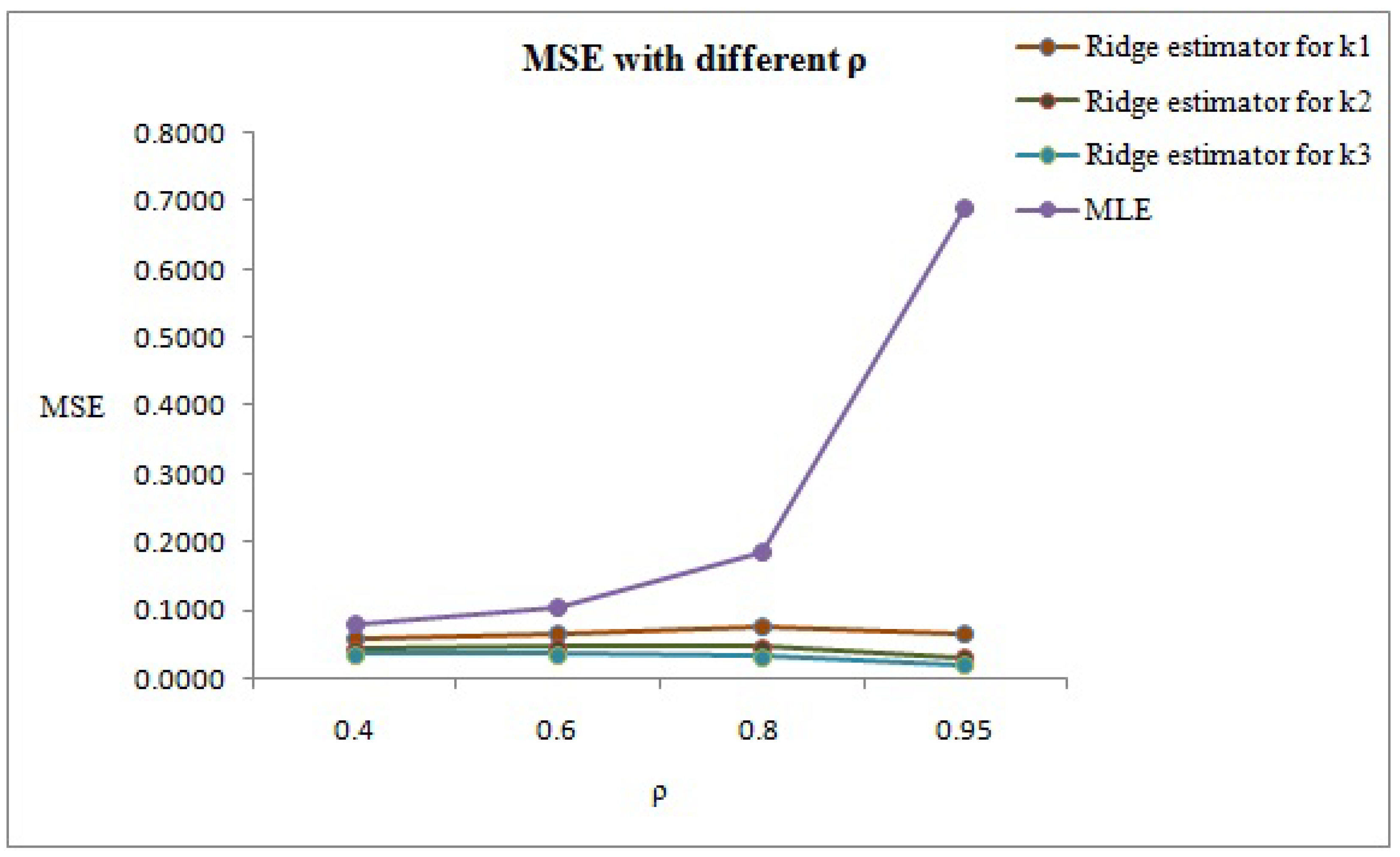
The findings of
Table 1,
Table 2 and
Table 3 demonstrate that the ridge estimators have a smaller MSE than ML. Among the three categories of
k, the ridge estimator performed better for
. In the case of moderate correlation (
), if
k changes from
to
then the percentage reduction will change from 37% to 66%. It is revealed from the
Table 1,
Table 2 and
Table 3 that if
increases then the percentage reduction in MSE also increases.
Figure 1 shows the graphical representation of MSE with respect to the deferent values of
.
4. Real Life Application
The proposed ridge regression estimator for the parametric frailty model is applied to a data set from the National Family Health Survey IIIrd Phase (NFHS III). The data set has 11,581 infants, out of which 10,448 infants are right censored. The response variable is the time of survival (in months) from the birth of the infant to the death of the infant. In this paper, the frailty model included 12 covariates of infant mortality, i.e., place of residence, breastfeeding, sex of infant, birth order, place of delivery, marital status of parents, tetanus toxoid (TT), antenatal care (ANC), age of mother, mother education, iron folic acid (IFA) and family size corresponding to each infant. Out of these covariates, TT and ANC are moderately correlated to each other and the correlation value is 0.6.
In some situations, the correlation cannot be considered as the standard measure of collinearity. The condition number is an alternative to measuring the collinearity. This study followed the Ozkale (2021) [
21] approach to measure the condition number. On the basis of this approach, the condition number is calculated for the matrix
, where
. The value of the condition number is 36.51, which is greater than 10. Therefore, collinearity is present in the data set [
22,
23].
Table 4 shows the distribution of births and deaths with different covariates in India 2005–2006. About 68% deaths occurred, where infants were not provided with breastfeeding. Approximately 53% infants were delivered at home, and the mothers were not educated in the same proportion. About 46% of births occurred when the size of the family was large, i.e., more than six members in the household. A total of 15%, 18% and 32% of mothers had not taken tetanus toxoid, antenatal care and IFA, respectively, during their pregnancy.
A frailty model is implemented on the data set and the results related to maximum likelihood and ridge estimates are summarized in
Table 5. A hazard ratio (exp(
)) less than one indicates a decreased death risk, while a greater than unity indicates an increased risk, and the interpretation of the hazard ratio is either the number of times the risk changes or the percentage change in the death risk.
Some significant results of the ridge regression are given as: Infants who were breastfeeding have a 99% lower death risk as compared to those who were not breastfeeding. Old married couples (more than nine years of marriage) have a 1.98 times higher risk of infant death as compared to newly married couples (0 to 4 years of marriage). If the age of the mother is more than 34 years, then the risk of infant death is increased by 1.5 times as compared to the infant of the reference category (mothers aged 18 to 24 years). The uneducated mother has a 9.82 times higher risk of infant death as compared to the highly educated mother. The risk of infant death is twice if the size of family is small (1 to 3 members in the household) and this risk is 28% lower for a large family (more than 6 members in the household) as compared to the reference category (4 to 6 members in the household). The estimated value of the is significantly non zero (), which means the unobserved variables have an impact on the survival times of the infants.
The results related to MSE corresponding to ridge estimators and the MLE are given in
Table 6, which shows that the MSE is the lesser for the ridge estimator as compared to the MLE, and the benefits are more when the ridge parameter is
.
5. Discussion and Conclusions
This paper generalized the approach of ridge regression in the frailty model. The frailty model deals with the time to event data and considered both factors (i.e., measurable and unmeasurable) simultaneously. Here, the parametric form of the frailty model is utilized. A simulation study is conducted and explained that the ridge estimator is more accurate and precise, as compared to MLE. The benefits are higher if the ridge parameter k is taken as .
The method is then applied to assess the risk of infant death in India. Data are taken from the third phase of NFHS and revealed that the proposed method produced more precise estimates as compared to MLE. Ridge estimates demonstrate that breastfeeding and mothers’ education are highly associated with infant mortality. The findings of this study demonstrates that maternal education is positively associated with infant mortality, i.e., the increment in the level of education reflects the decrement in the infant mortality; these results are significant. There is a high risk of infant death if the mother’s age is less than 18 years, and the reason for this finding may be considered as the complications of delivery, premature birth, pregnancy and some other related issues of teenagers. A bigger family size has a positive impact on infant death.


