Short- and Medium-Term Power Demand Forecasting with Multiple Factors Based on Multi-Model Fusion

Abstract

With the continuous development of economy and society, power demand forecasting has become an important task of the power industry. Accurate power demand forecasting can promote the operation and development of the power supply industry. However, since power consumption is affected by a number of factors, it is difficult to accurately predict the power demand data. With the accumulation of data in the power industry, machine learning technology has shown great potential in power demand forecasting. In this study, gradient boosting decision tree (GBDT), extreme gradient boosting (XGBoost) and light gradient boosting machine (LightGBM) are integrated by stacking to build an XLG-LR fusion model to predict power demand. Firstly, preprocessing was carried out on 13 months of electricity and meteorological data. Next, the hyperparameters of each model were adjusted and optimized. Secondly, based on the optimal hyperparameter configuration, a prediction model was built using the training set (70% of the data). Finally, the test set (30% of the data) was used to evaluate the performance of each model. Mean absolute error (MAE), root mean square error (RMSE), mean absolute percentage error (MAPE), and goodness-of-fit coefficient (R^2) were utilized to analyze each model at different lengths of time, including their seasonal, weekly, and monthly forecast effect. Furthermore, the proposed fusion model was compared with other neural network models such as the GRU, LSTM and TCN models. The results showed that the XLG-LR model achieved the best prediction results at different time lengths, and at the same time consumed the least time compared to the neural network model. This method can provide a more reliable reference for the operation and dispatch of power enterprises and future power construction and planning.

1. Introduction

Electricity is one of the most important basic energy sources in the world. It can provide basic support for industrial production and processing, and sustain people’s daily life. Since there is no high-quality storage carrier for electric energy at this stage, low storage efficiency occurs when battery packs or pumped energy storage power stations are solely adopted. Therefore, power generation should be roughly equal to the demand, otherwise it will lead to consequences like the wasting of resources [1]. In addition, thermal power generation is the main way of generating electricity in most parts of the world, so excessive power generation will also cause serious environmental pollution. Furthermore, in the course of modern electric power development, there have been numerous incidents of insufficient power supply and shortage of power which seriously affected China’s economic and social development. In the United States, from 14 February 2021 on, widespread rolling blackouts in Texas amid extremely cold weather left millions of people living without electricity. About 30% of the power generating units in Texas were off-grid during the extreme weather. Moreover, starting on 23 September 2021, many places in Northeastern China issued notifications of power rationing and implemented the policy of orderly power consumption for non-residents. The occurrence of the above-mentioned events was caused by insufficient power supply to a certain extent. However, at the same time there existed inappropriate prior power dispatching caused by the inaccurate estimation of power demand. It can be seen that the supply capacity of the power industry is closely related to the national macroeconomic development. If the total power required by a population can be predicted in advance, the waste of power resources can be avoided to the greatest extent. The economic benefits of power enterprises can be improved and damage to the environment can be reduced. The ever-increasing demand for power resources has also led to higher requirements for power operation and management. Any deviation will bring incalculable losses. At this stage, China’s “smart grid” is developing at rapid speed. The construction of power facilities, power supply and power sales all depend on accurate forecasts of power demand [2].

Power demand forecasting refers to making predictions about the electricity demand of the electricity market in the future. Generally, it is divided into three categories according to the time span: short-term forecasting, medium-term forecasting and long-term forecasting. Short-term forecasting generally refers to forecasting using the day as the smallest unit. Commonly used methods include the linear recursive least squares method and the state space method based on a Kalman filter, etc. [3]. Medium-term forecasting generally refers to forecasting based on months or quarters as the smallest unit. Commonly used methods include the seasonal index method and the ARIMA model method [4]. Long-term forecasting generally refers to forecasting by year as the smallest unit, and the commonly used methods mainly include the moving average method and the neural network method [5]. From the perspective of forecasting characteristics, the amount of historical data utilized in short-term forecasting is relatively large, and it will be affected differently during different holidays, so comprehensive consideration is needed in forecasting; the data of medium-term forecasting has obvious seasonal characteristics, so it is necessary to carry out forecasting in combination with this feature. For long-term forecasting, due to limited historical data and many external interference factors, it is necessary to fully mine data characteristics during forecasting so as to obtain better forecasting results. With regard to short-term forecasting, it can provide corresponding decision-making guidance for real-time grid dispatching [6]; while long-term forecasting can provide data support for expansion of both the grid and its capacity on the basis of guiding power system planning and construction [7].

In the past, power forecasting technology mainly applies to time series in statistics [8], multiple linear regression [9], ARIMA [10], and other methods. Due to their simplicity in theory and because they require less amounts of calculation, these methods are more frequently applied in the initial research on power forecasting. However, it is to carry out forecasting in combination with external factors, thus the forecasting accuracy is largely limited, which makes it difficult to meet the actual needs. Since the 1980s, researchers begin to introduce intelligent algorithms from other fields into electricity forecasting. In 1991, PARK D. C. and other scholars first used artificial neural networks for power prediction and achieved satisfactory results [11]. Compared with traditional statistical prediction methods, artificial intelligence technology can analyze and learn from a large amount of data in a short period of time, and significantly improve the prediction accuracy, which has obvious advantages.

At present, the methods adopted by domestic researchers more often refer to neural networks [12,13,14], support vector machines [15], and the joint model [16]. Reference [17] proposes a power demand forecasting model based on a second-order gray neural network. First, the wavelet sequence is used to perform stationarity processing on the original data set, and then the power demand is predicted using a second-order gray neural network. Reference [18] adopts the grayscale model of a neural network to predict the power demand, and obtains a relatively good prediction effect. Reference [19] proposes a LSSVM_PSO model for power demand forecasting. The model utilizes a particle swarm optimization algorithm to adjust the learning rate to reduce the prediction error of the support vector machine and improve its reliability. Compared with the least squares support vector machine, this method achieves higher convergence rates and prediction performance. Reference [20] combines the feedback of the neural network and ARMA models to predict the power generation of wind power plants, and this model achieves high accuracy and interpretability. Reference [21] proposes a power load forecasting model based on extreme gradient enhancement to solve the problem whereby traditional forecasting models have difficulty in dealing with massive data when power data grows exponentially in some cases. Through the analysis of meteorological factors and the long-term regularity of the daily power load, the model achieves higher prediction accuracy and smoother prediction error compared with traditional machine algorithms. Reference [22] combines the two models of Xgboost and ARMA, and uses the power consumption data of enterprise users to make predictions. Through a series of comparative experiments, it is found that this method achieves more accurate prediction results than traditional methods.

Through the above analysis, and in view of the problems that short- and medium- term power data is less informative and difficult to predict, after considering the impact of meteorological factors on power consumption, this paper integrates LGB, XGB and GBDT, and fully explores the correlation between electricity demand and weather data through the integrated model. The model is trained by using the time series relationship existing in the data so as to obtain a more accurate prediction effect.

2. Data Source and Data Processing

2.1. Data Source

The data in this paper came from the 13-month electricity consumption data of a city in China published on the Internet. The original data set contains five attribute items, including historical electricity consumption, temperature, humidity, wind speed and rainfall. All data was collected every 15 min, that is, the data of five attribute items was recorded once every 15 min. The specific data set is shown in

Table 1. Weather and Electricity Consumption Data.

Date	Temperature				Humidity				Wind Speed
$Time$	00:00	00:15	…	23:45	00:00	00:15	…	23:45	00:00	00:15	…	23:45
Year 1 Day 1	14.29	14.12	…	13.28	47.97	48.42	…	74.28	3.5	3.3	…	1.6
Year 1 Day 2	17.59	17.37	…	16.74	47.42	48.46	…	71.16	1.28	1.14	…	0.27
Year 1 Day 3	20.89	20.72	…	16.72	48.12	48.84	…	70.66	0.94	0.91	…	0.23
…	…	…	…	…	…	…	…	…	…	…	…	…
Year 2 Day 31	18	18	…	18.25	80	80.25	…	54.75	3	3.25	…	5.75
Date	Rainfall						Electricity consumption
$Time$	00:00	00:15		…	23:45		00:00	00:15		…	23:45
Year 1 Day 1	0	0		…	0		45,208.29	44,342.25		…	40,985.48
Year 1 Day 2	0	0		…	0		39,887.65	39,531.59		…	55,027.02
Year 1 Day 3	0	0		…	0		53,562.43	52,851.47		…	57,401.79
…	…	…		…	…		…	…		…	…
Year 2 Day 31	0	0		…	0		35,890.91	35,227.22		…	34,784.86

, where time represents the time of data recording.

In order to verify the effectiveness of the model, the data set was divided into a training set and a test set before model training according to the power demand forecasting tasks of different durations. The training set accounted for 70% of the original data, and the test set accounted for 30%.

2.2. Data Cleaning

The data item of electricity consumption in the data used in this paper was analyzed, and a data trend diagram was drawn, as shown in Figure 1. It can be seen that the data fluctuated significantly since the 41st day of Year 1. Since the original data came from a certain city in China, it was speculated that this period should be during the Chinese Lunar New Year, when a large number of urban migrant workers returned to their hometowns to celebrate the New Year, and a large number of enterprises and institutions stopped work and production during this period, resulting in large fluctuations in electricity consumption. In order to reduce the impact of the abnormal fluctuation on prediction results, this paper classified the data of 15 days after the 41st day of Year 1 as abnormal data and deleted it from the data set.

2.3. Data Normalization

The main goal of data normalization was to scale the original data within a fixed interval according to certain rules to eliminate the influence of different data dimensions in the original data so as to ensure that the model training results were not affected by the original data dimensions. In this paper, according to Equation (1), five attribute items including electricity consumption, temperature, humidity, wind speed and rainfall in the original data were normalized to the [0,1] interval [23].

$${\widehat{x}}_i=\frac{x_i-X_{\min }}{X_{\max }-X_{\min }}$$

(1)

In the equation, ${\widehat{x}}_i$ is the normalized value of the $i$th value of the sample, $x_i$ is the $i$th value of the sample, $X_{\min }$ is the minimum value of the sample, and $X_{\max }$ is the maximum value of the sample.

3. Methodology

3.1. Boosting and Decision Tree

Ensemble learning completes the learning task by constructing and combining multiple learners. By combining multiple learners, it is often possible to obtain significantly better generalization performance compared to a single learner. There are three common ensemble learning ideas, including bagging, boosting, and stacking.

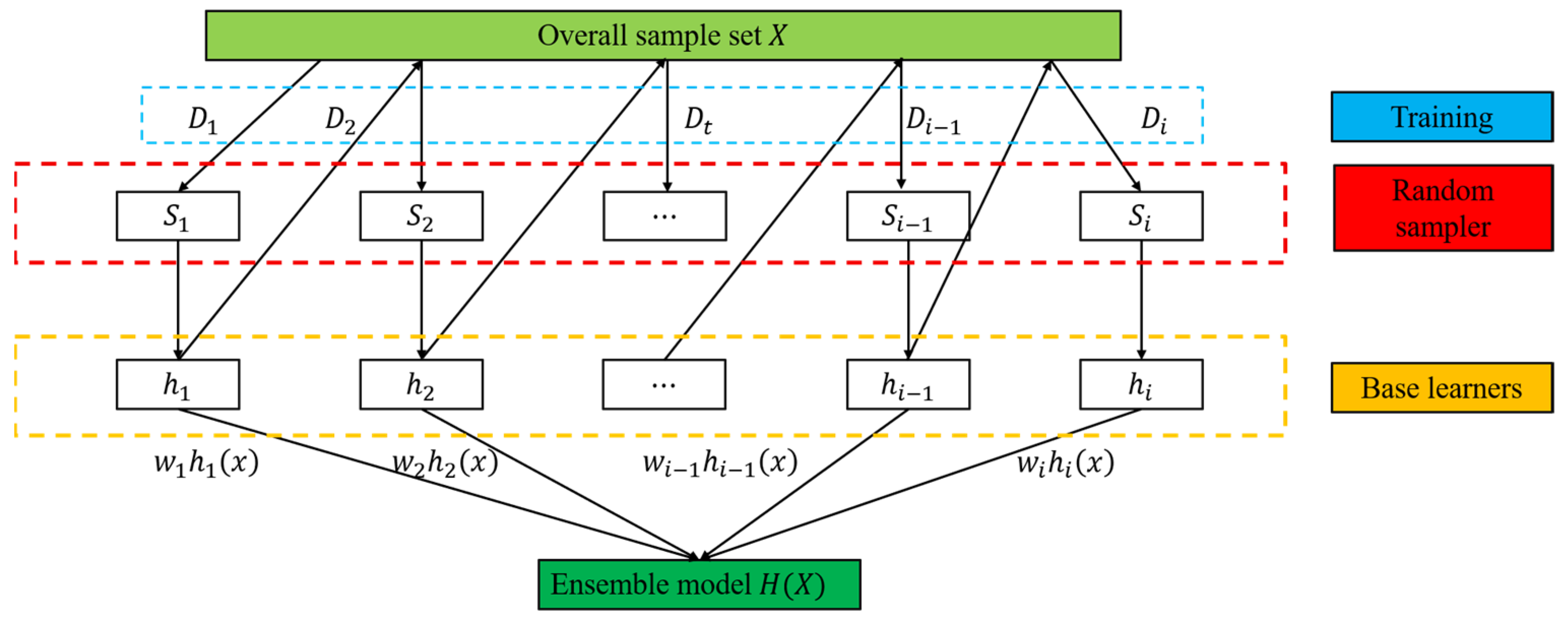
Boosting is a kind of algorithm that can upgrade a weak learner to a strong learner. The working mechanism is as follows: firstly, train a base learner from the initial training set, and then adjust the distribution of training samples according to the performance of the base learner, so that the training samples made by the previous base learner will receive more attention in the follow-up. The next base learner is then trained based on the adjusted sample distribution. This is repeated until the number of base learners reaches the specified value $N$, and finally the $N$ base learners are weighted together. The flow chart of the algorithm is shown in Figure 2:

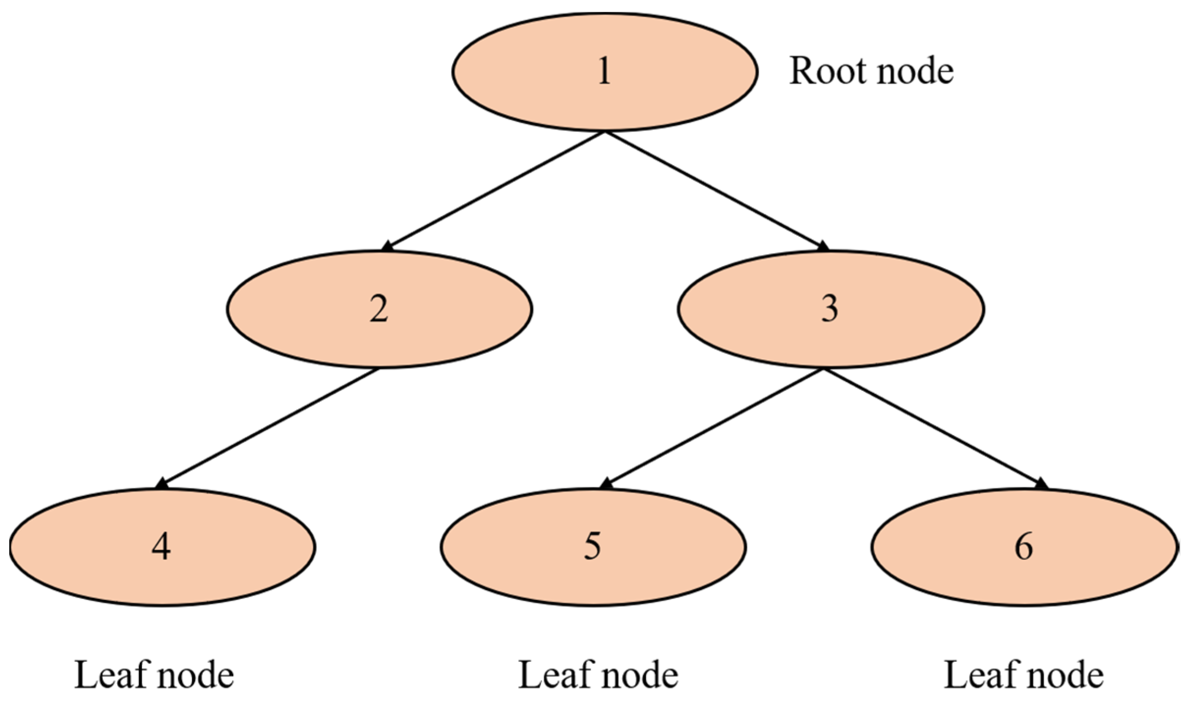
A decision tree is an important model in ensemble learning, and its core is a tree structure, as shown in Figure 3. The figure represents the mapping relationship between object attributes and object values. The root node and inner node represent the segmentation of features, and each branch denotes the output of the feature corresponding to the parent node in the regional space here.

Decision trees are generally divided into classification trees and regression trees. Classification trees are often used in class division, while regression trees are often used in numerical prediction [24]. During the growth of the regression tree, each leaf node can get a predicted value, and the threshold of each feature value is exhausted during segmentation. The optimal segmentation variable and optimal segmentation point are found by minimizing the squared error, and then the minimized square error is utilized to find the most credible segmentation basis so as to ensure that the predicted value of the current branch node is unique, or at a certain artificial threshold. If the data of each leaf node is not unique, the average value of the node data is used as the predicted value.

The growth of the above regression tree generally has the following five steps:

Step 1: Enter the training data set, as follows:

$$T=\left\{\left(x_1,y_1\right),\left(x_2,y_2\right),\cdots \left(x_n,y_n\right)\right\},x_i\in X\in R^n,y_i\in Y\in R^n$$

(2)

Step 2: Traverse all feature variables $j$. When the fixed segmentation variable $j$ is encountered, segmentation point $s$ is scanned.

$${\min }_{j,s}[{\min }_{c_1}{{\displaystyle \sum }}_{x_i\in R_1\left(j,s\right)}{\left(y_i-c_1\right)}^2+{\min }_{c_2}{{\displaystyle \sum }}_{x_i\in R_2\left(j,s\right)}{\left(y_i-c_2\right)}^2]$$

(3)

At this time, the optimal segmentation variable $j$ and the segmentation point $s$ with the smallest overall square error loss are obtained.

Step 3: After the segmentation scheme at the value $s$ of the first attribute $j$ is obtained, calculate the output of the two sub-regions:

$$R_1\left(j,s\right)=\{x|x^{\left(j\right)}\le s\}$$

(4)

$$R_2\left(j,s\right)=\{x|x^{\left(j\right)}\le s\}$$

(5)

Step 4: Continue to call steps 2 and 3 for the two sub-regions to find the optimal variable characteristics of each branch node. The growth of the regression tree ends when all regions meet the threshold or exhaust all attributes for its growth.

Step 5: The input space is divided into M regions, $R_1,R_2,\cdots ,R_M$, and there is a fixed output value $c_m$ in each divided unit region. The final decision tree is generated as follows:

$$f\left(x\right)={{\displaystyle \sum }}_{m=1}^M{c}_{m}I\left(x\in R_m\right)$$

(6)

3.2. Gradient Boosting Decision Algorithm

The gradient boosting decision algorithm is a representative algorithm in the boosting series of algorithms, which consists of multiple decision trees, and the conclusions of all trees are accumulated as the final answer [25]. The main idea of the gradient boosting decision tree is to take advantage of the squared error to denote the loss function, in which each regression tree learns the conclusions and residuals of all previous trees, and fits a current residual regression tree. The residual is the difference between the true value and the predicted value. The boosting tree is the accumulation of the regression trees generated by the entire iterative process. However, the gradient boosting decision tree requires that the weak learner must be a CART regression tree model, and GBDT requires that the sample loss predicted by the model be as small as possible during model training. The process of using GBDT as a regression algorithm to predict the power demand is as follows:

Assume that the training set samples are $T=\left(x_1,y_1\right),\left(x_2,y_2\right),\dots ,\left(x_m,y_m\right)$, the maximum number of iterations is $T$, the loss function commonly uses mean square error function $L\left(y,f\left(x\right)\right)={\left(y-f\left(x\right)\right)}^2$, and the output is the strong learner $f\left(x\right)$. The regression algorithm process is as follows:

Step 1: Initialize the weak learner. The mean of $C$ can be set to the mean of the sample $y$.

$$f_0\left(x\right)=\arg \min {\displaystyle \sum }_{i=1}^{m}L\left(y_i,c\right)$$

(7)

Step 2: For the number of iterations $t=1,2,3\dots T$, calculate the negative gradient for samples $i=1,2,3\dots m$.

$$r_{ti}=-{\left[\frac{\partial L\left(y_i,f\left(x_i\right)\right)}{\partial f\left(x_i\right)}\right]}_{f\left(x\right)=f_{t-1}\left(x\right)}$$

(8)

Step 3: Use $\left(x_i,r_{ti}\right)i=1,2,3,\dots ,m$ to fit a CART regression tree to get the $t$th regression tree. Its corresponding leaf node area is $R_{tj},j=1,2,3,\dots ,J$, where $J$ is the number of leaf nodes of the regression tree $t$.

Step 4: With regard to the leaf region $j=1,2,3,\dots ,J$, there is the best fitting value at this time.

$$c_{tj}=\arg \min {\displaystyle \sum }_{x_i\in R_{tj}}L\left(y_i,f_{t-1}\left(x_i\right)+c\right)$$

(9)

Step 5: Update the strong learner.

$$f_t\left(x\right)=f_{t-1}\left(x\right)+{{\displaystyle \sum }}_{j=1}^J{c}_{tj},I\left(x\in R_{tj}\right)$$

(10)

Finally, the expression of the strong learner $f\left(x\right)$ is obtained:

$$f\left(x\right)=f_T\left(x\right)=f_0\left(x\right)+{{\displaystyle \sum }}_{t=1}^T{{\displaystyle \sum }}_{j=1}^J{c}_{tj},I\left(x\in R_{tj}\right)$$

(11)

GBDT can be applied to most regression problems [26,27]. For dense data such as electricity demand, a variety of distinguishing features and feature combinations can be found through this model, which has strong generalization and expression ability to achieve a better fitting effect.

3.3. LightGBM Model

In order to improve model training efficiency and reduce memory consumption, based on the traditional GBDT algorithm, the Light Gradient Boosting Machine (LightBGM) algorithm is proposed [28]. The pre-sorting algorithm commonly used in the boosting algorithm performs feature selection and splitting. This method can accurately find the splitting point, but the memory usage and computational cost are high. Therefore, the LightBGM algorithm uses Histogram to improve the speed of processing training samples. The Histogram algorithm constructs a piecewise function in advance before training, converts continuous eigenvalues into $K$ discrete bin values, and then establishes a histogram containing $K$ items. The constructed histogram is utilized to traverse the training samples. During this process, the LightBGM algorithm accumulates statistics in the histogram according to $K$ discrete values and finally finds the best split point from the discrete values. This method can significantly reduce the computational memory and computational cost, and significantly improve the computational speed.

In addition, the leaves of the GBDT algorithm use a level-wise growth method, which does not distinguish the leaves of the same layer. However, in fact, the split of many leaves brings a low gain, which brings the waste of computing resources and memory resources [29]. In response to this problem, the LightBGM algorithm adopts a more efficient Leaf-wise algorithm that grows according to leaves. It splits by finding the largest splitting gain from a certain layer of leaves and repeats it continuously, which enables the algorithm to achieve higher accuracy under the same number of splits. Meanwhile, overfitting can be avoided by limiting the depth of the tree when the sample size is small.

It can be seen from the above that the LightBGM algorithm, based on the core idea of the GBDT algorithm, improves the feature splitting process and tree growth method by introducing a new method, which makes the model simpler, requires less computational cost, and achieves more accurate predictions.

3.4. XGBoost Algorithm

Based on the decision tree boosting optimization model, the XGBoost algorithm converts weak learners into strong learners through iteration [29]. In the XGBoost algorithm, the CART regression tree is used as a weak learner to first determine the optimal structure of the tree, such as the number of leaf nodes and the depth of the tree. Next, the distributed forward additive model is adopted. Each time a single tree is generated, the weight of the last misclassified data is increased and used for the current tree, and the overall error of the model is gradually reduced by continuously adding trees until the end of training [30].

When the XGBoost algorithm is adopted to train samples, the model for each tree is as follows:

$$f_t\left(x\right)=w_{q\left(x\right)},w\in R^T,q:R^d\left\{1,2,\cdots ,M\right\}$$

(12)

In the equation, $w$ is the leaf node score value. $x$ represents the input sample data, $q\left(x\right)$ denotes the leaf node corresponding to the sample $x$, and $M$ is the number of leaf nodes of the tree. The equation for adding the $m$th tree to the model is as follows:

$${\hat{y}}_i^{\left(l\right)}={\displaystyle \sum }_{k=1}^m{f}_k\left(x_i\right)={\hat{y}}_i^{\left(m-1\right)}+f_m\left(x_i\right)$$

(13)

To train a single CART tree [31], the objective function needs to be determined first:

$$Obj\left(\theta \right)={\displaystyle \sum }_{i=1}^{n}L\left(y_j,{\hat{y}}_i^{\left(l\right)}\right)+{\displaystyle \sum }_{k=1}^m\Omega \left(f_K\right)$$

(14)

The objective function is divided into two parts, including loss function $L$ and regularization $\Omega$. For regression, the loss of the square of the residual between the predicted value and the true value, that is, the L2 loss, is generally used to evaluate the degree of model fitting, and the regularization term acts as a penalty term for the model to prevent overfitting. The regularization term is defined as:

$$\Omega \left(f_m\right)=rM+\frac{1}{2}\lambda {\displaystyle \sum }_{j=1}^M{w}_j^2$$

(15)

In the equation, $M$ refers to the number of leaf nodes and $w_j$ refers to the $\mathrm{L}2$ regularity of leaf node scores. $r$ and $\lambda$ are used to control the complexity of the tree. From this, the regularization term can be calculated. Equations (12), (13), and (15) are brought into the objective function, and the second-order Taylor formula is used to obtain the form of the leaf node of the $m$th tree, which is as follows:

$$\begin{array}{l}Ob{j}^m\left(\theta \right)={\displaystyle {\displaystyle \sum }_{i=1}^n}\left[g_i{w}_{q\left(x_i\right)}\frac{1}{2}{h}_i{w}_{q\left(x_i\right)}^2\right]+\frac{1}{2}\lambda {\displaystyle {\displaystyle \sum }_{j=1}^M}{w}_j^2\\ \hspace{1em}\hspace{1em}={\displaystyle \sum }_{j=1}^M\left[\left({\displaystyle \sum }_{i\in I_j}{g}_i\right)w_j+\frac{1}{2}\left({\displaystyle \sum }_{i\in I_j}{h}_i+\lambda \right)w_j^2\right]+rM\end{array}$$

(16)

Let $G_j={\displaystyle \sum }_{i\in I_j}{g}_i$, $H_j={\displaystyle \sum }_{i\in I_j}{h}_i$. Bring them into Equation (16) and obtain the partial derivative of the objective function with respect to $w_j$. Set the value of the derivative function to 0, and obtain:

$$w_j^{*}=-\frac{G_j}{H_j+\lambda }$$

(17)

Bring it into the objective function and obtain:

$$Ob{j}^{*}=-\frac{1}{2}{{\displaystyle \sum }}_{j=1}^M\frac{G_j^2}{H_j+\lambda }+rM$$

(18)

This paper used $Ob{j}^{*}$ to evaluate the quality of a single CART regression tree structure. XGBoost enumerated the splitting schemes of all features from the tree with a depth of 0 and calculated its objective function value to determine the optimal structure of the tree. When the tree reached the maximum depth and the sum of the sample weights was less than the set threshold, the establishment of the decision tree was stopped. The sampling ratio of each tree was controlled by the set parameters, and the structure training process of a tree was finally optimized through parameter adjustment.

XGBoost applied boosting to carry out the next round of training after training one tree, obtaining the optimized training model structure through continuous iteration. After one iteration, XGBoost multiplied the weight of the leaf node and the learning rate, thereby weakening the influence of each tree and providing a larger learning space for subsequent trees. Finally, the optimal number of iterations of the model was determined, and the training of the model was completed.

3.5. LR Model

The LR model is mainly represented by a conditional probability distribution $P\left(Y|X\right)$ in the form of a parameterized logistic distribution. Among them, the value range of $X$ as a random variable is a real number, and the value range of $X$ as a random variable is 1 or 0. The conditional distribution of the LR model is as follows:

$$P\left(Y=1|x\right)=\frac{exp\left(w·x+b\right)}{1+exp\left(w·x+b\right)}$$

(19)

$$P\left(Y=0|x\right)=\frac{1}{1+exp\left(w·x+b\right)}$$

(20)

In the equation, $x\in R^n$ refers to the input, $Y\in \left\{0,1\right\}$ refers to the output, $w\in R^n$ and $b\in R$ are the parameters, $w$ is the weight vector, $b$ is the bias, and $w·x$ is w and the inner product of $x$.

For a given input $x$, $P\left(Y=1|x\right)$ and $P\left(Y=0|x\right)$ can be solved according to Equations (19) and (20). Logistic regression compares two conditional probability values and finds a class with a larger probability value, thereby assigning input $x$ to that class.

The weight vector $w$ and the input vector $x$ are extended to get $w={\left(w^{\left(1\right)},w^{\left(2\right)},\cdots w^{\left(n\right)},b\right)}^T$, $x={\left(x^{\left(1\right)},x^{\left(2\right)},\cdots x^{\left(n\right)},1\right)}^T$. At the moment, the LR model is as follows:

$$P\left(Y=1|x\right)=\frac{\exp \left(w·x\right)}{1+\exp \left(w·x\right)}$$

(21)

$$\left(Y=0|x\right)=\frac{1}{1+\exp \left(w·x\right)}$$

(22)

The probability of an event occurring divided by the probability of an event not occurring is the probability of the event. At this time, assume that the probability of an event occurring is $p$, the probability of it not occurring is $1-p$, thus the probability of the event is $\frac{p}{1-p}$. The logarithmic probability of the event is as follows, which can also be called the logit function.

$$\mathrm{logit}\left(p\right)=\log \frac{p}{1-p}$$

(23)

For logistic regression, the following equation can be obtained from Equations (21) and (22).

$$\log \frac{P\left(Y=1|x\right)}{1-P\left(Y=1|x\right)}=w·x$$

(24)

It can be seen from the above equation that in the LR model, the logit function with the output $Y=1$ has a linear relationship with the input $x$. The value domain of the linear function $w·x$ is the real number domain, and the input $x$ can be split by a linear function.

Since $x\in R^{n+1}$, $w\in R^{n+1}$, the linear function $w·x$ can be converted into a probability by taking advantage of Equation (19):

$$\left(Y=1|x\right)=\frac{\exp \left(w·x\right)}{1+\exp \left(w·x\right)}$$

(25)

When the linear function $w·x$ infinitely approaches positive infinity, the value of the conditional probability approaches 1; when the linear function $w·x$ infinitely approaches negative infinity, the value of the conditional probability approaches 0.

A training dataset $T=\left(x_1,y_1\right),\left(x_2,y_2\right),\dots ,\left(x_m,y_m\right)$, where $x_i\in R^n$, $y_i\in \left\{0,1\right\}$, is given. The maximum likelihood estimation method is used here to estimate the LR model parameters.

$$\left(Y=1|x\right)=\pi \left(x\right)$$

(26)

$$P\left(Y=0|x\right)=1-\pi \left(x\right)$$

(27)

At this moment, the likelihood function is ${{\displaystyle \sum }}_{i=1}^m{\left[\pi \left(x_i\right)\right]}^{y_i}{\left[1-\pi \left(x_i\right)\right]}^{1-y_i}$, and the log-likelihood function is

$$\begin{array}{l}L\left(w\right)={\displaystyle {\displaystyle \sum }_{i=1}^m}\left[y_i\log \pi \left(x_i\right)+\left(1-y_i\right)\log \left(1-\pi \left(x_i\right)\right)\right]\\ \hspace{1em}\hspace{1em}={\displaystyle {\displaystyle \sum }_{i=1}^m}\left[y_i\log \frac{\pi \left(x_i\right)}{1-\pi \left(x_i\right)}+\log \left(1-\pi \left(x_i\right)\right)\right]\\ \hspace{1em}\hspace{1em}\hspace{1em}\hspace{1em}={\displaystyle {\displaystyle \sum }_{i=1}^m}\left[y_i\left(w·x_i\right)-\log \left(1+\exp \left(w·x_i\right)\right)\right]\end{array}$$

(28)

The estimated value of $w$ can be obtained by solving the local maximum of Equation (28).

Next, we optimize the objective function, which is the log-likelihood function. In logistic regression, gradient descent and quasi-Newton methods are often used. Assume that $\widehat{w}$ is the maximum likelihood estimate of $w$, and the resulting LR model is

$$P\left(Y=1|x\right)=\frac{\exp \left(\widehat{w}·x\right)}{1+\exp \left(\widehat{w}·x\right)}$$

(29)

$$\left(Y=0|x\right)=\frac{1}{1+\exp \left(\widehat{w}·x\right)}$$

(30)

Due to the limited learning ability of the LR model, it is often necessary to combine it with other models [32]. Corresponding feature combinations are obtained by other models through training, and then the LR model gives the corresponding predicted values.

4. Power Demand Forecasting Model Based on Stacking

In view of the fact that no single model can meet the requirements of training performance and stability well, this paper attempts to use the Stacking to synthesize the advantages of various boosting models [33]. Moreover, combining it with the LR regression model enables the fusion model to have strong discrimination and stability, and does not require too frequent iterations on the basis of achieving good results.

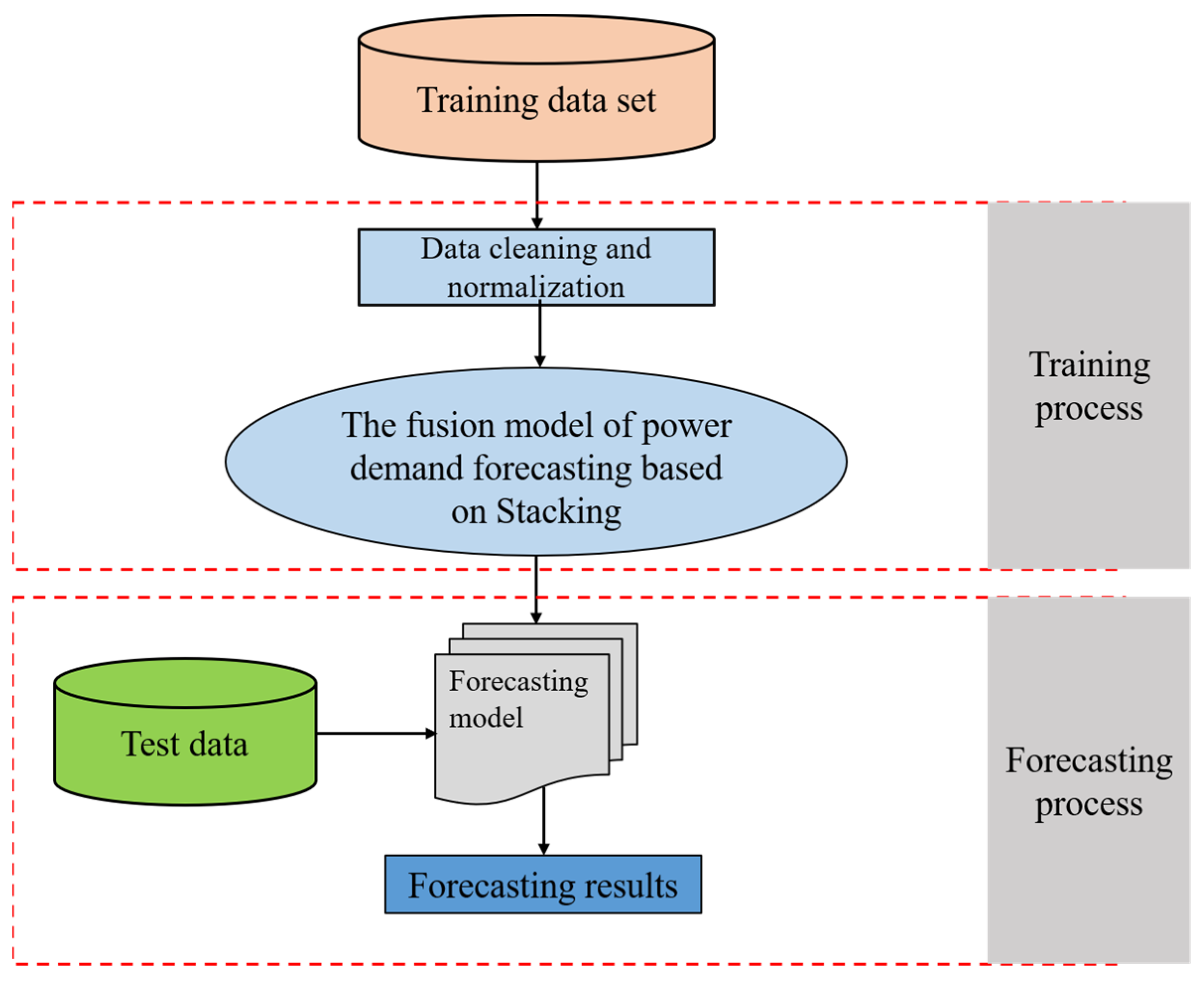
The overall design of model training and testing in this study is shown in Figure 4. First, the original data is cleaned and normalized, and then the power demand forecasting model based on stacking is trained to obtain the corresponding forecasting model. Next, the test data is used for prediction.

The process of model training is then described in detail. Through the previous analysis, it can be found that the power demand data involved in this study has strong regularity in the time series when they are divided by day, month and season after the data on special holidays is removed. Meanwhile, the amount of data is limited, so the model based on decision tree is more suitable for solving this kind of problem. Three models, including GBDT, XGBoost and LightGBM, have their own advantages and disadvantages in predicting different scenarios. The fusion of the three models can achieve a joint gain effect. Stacking is an ensemble framework for hierarchical models [34]. The first layer is composed of a number of different base learners. This paper selected three models, including GBDT, XGBoost and LightGBM. When each model was adjusted to achieve good results, they were integrated to predict, thereby reducing the deviation of the model and achieving better results. The LR regression model was selected for the second layer, which further avoided the occurrence of overfitting, effectively reduced the variance of the model, and made the model more stable. The specific steps of the power demand forecasting model based on stacking are as follows:

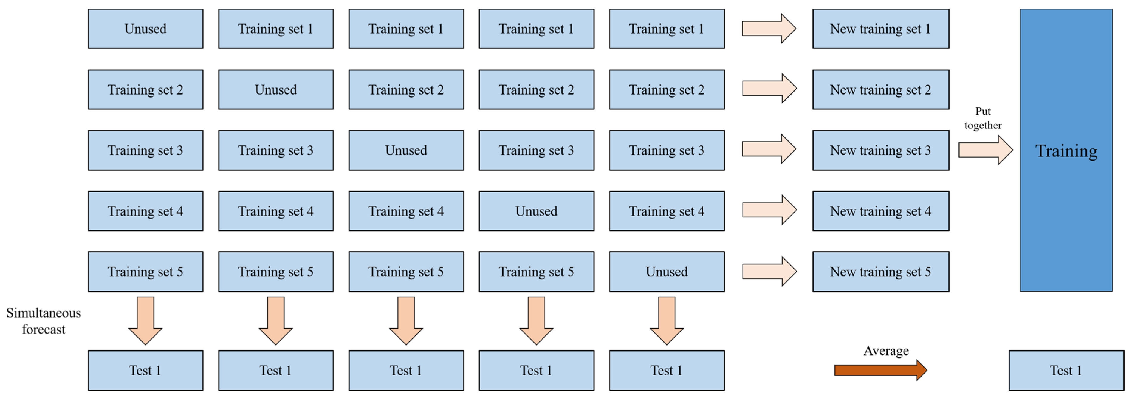
Step 1: First, the overall data set consisting of meteorological factor and power demand was divided into training data (training set) and prediction data (testing set). Then the training samples were divided into $k$ groups of data with the same amount.

Step 2: The training data set was trained multiple times with each base learner. Each training utilized $k-1$ pieces of data as training samples, and the remaining one was used as a validation set. The data of meteorological factor in the validation set was utilized to predict power demand, so as to obtain $k$ copies of the prediction data through the validation set. In addition, the prediction samples would be predicted during each training process to obtain $k$ copies of prediction data. It should be noted that only the training set needs to do this step. The validation set and test set do not need it.

Step 3: Combine the $k$ pieces of prediction data obtained through the validation set to get new training sample data. The obtained $k$ pieces of prediction data were averaged to obtain new prediction data. The specific process is shown in Figure 5.

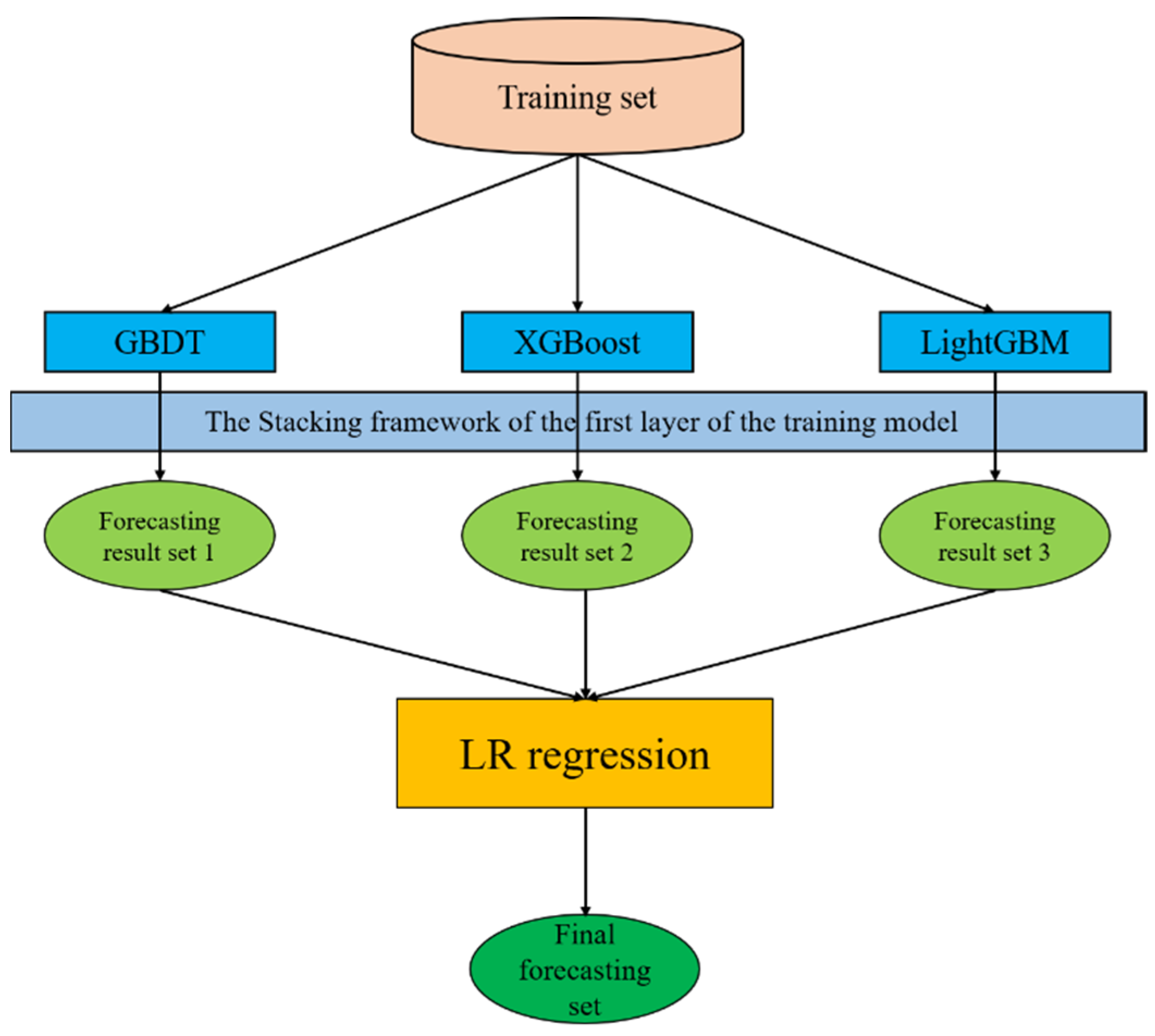
Step 4: Input the data obtained in Step 3 into the second layer, and finally get the final prediction result. The process is shown in Figure 6.

The power demand model constructed in this paper used GBDT, XGBoost and LightGBM, the three boosting models in the first layer of the stacking framework. The second layer of the stacking framework adopted the LR model to directly output the prediction results. The overall framework of the model is shown in Figure 6.

The optimal parameters of each basic model are summarized in

Table 2. Summary of Hyperparameters of Each Basic Model.

Algorithm	Hyperparameters	Meanings	Optimal Values
GBDT	n_estimators	Number of trees	100
	Learing_rate	Shrinkage coefficient of each tree	0.1
	Max_depth	Maximum depth of a tree	5
	Min_samples_leaf	Minimum number of samples for leaf nodes	1
	Min_samples_split	Minimum number of samples for nodes split	2
	subsample	The number of samples used by the base model during training	0.85
XGBoost	n_estimators	Number of trees	120
	Learing rate	Shrinkage coefficient of each tree	0.1
	Max_depth	Maximum depth of a tree	5
	Colsample_bytree	Subsample ratio of columns for tree construction	0.9
	Subsample	Subsample ratio of training samples	0.8
	Gamma	Penalty items cut off for each additional leaf	0
LGB	n_estimators	Number of trees	100
	learing rate	Shrinkage coefficient of each tree	0.1
	Max_depth	Maximum depth of a tree	1
	num_leaves	Number of leaves for each tree	63

. In this study, some key hyperparameters in GBDT, XGBoost, and LightGBM algorithms were adjusted, as shown in Table 2. Table 2 also explains the specific meaning of these hyperparameters. According to the maximum average precision, the best value of each set of hyperparameters is obtained, as shown in Table 2.

5. Results and Analysis

5.1. Evaluation Indicators

Power demand forecasting calculates the power consumption demand for a period of time in the future based on the internal relationship between the historically recorded power consumption data and the corresponding meteorological information. The estimated power consumption demand often has some errors compared with the actual power demand. The smaller the error, the higher the accuracy of the model, and the closer the fit between estimated and actual power consumption demand curve, which means the better performance of the model. Therefore, the objective evaluation of the model is of great significance for analyzing the quality of the model.

In this paper, four commonly used model evaluation indicators, including mean absolute error (MAE), root mean square error (RMSE), mean absolute percentage error (MAPE), and goodness-of-fit coefficient ($R^2$) were used to evaluate a single deterministic model. The formulas are as follows:

$$MAE=\frac{1}{n}{{\displaystyle \sum }}_{n=1}^n\left|Q_{obs,n}-Q_{sim,n}\right|$$

(31)

$$RMSE=\sqrt{\frac{1}{n}{{\displaystyle \sum }}_{n=1}^n{\left(Q_{obs,n}-Q_{sim,n}\right)}^2}$$

(32)

$$MAPE=\frac{1}{n}{{\displaystyle \sum }}_{n=1}^n\left|\frac{Q_{obs,n}-Q_{sim,n}}{Q_{obs,n}}\right|$$

(33)

$$R^2=1-\frac{{{\displaystyle \sum }}_{n=1}^n{\left(Q_{sim,n}-{\overline{Q}}_{obs}\right)}^2}{{{\displaystyle \sum }}_{n=1}^n{\left(Q_{obs,n}-{\overline{Q}}_{sim}\right)}^2}$$

(34)

In the formula, $Q_{sim,n}$ represents the predicted value, $Q_{obs,n}$ represents the true value, ${\overline{Q}}_{sim}$ represents the mean of the predicted value, and ${\overline{Q}}_{obs}$ represents the mean of the actual value.

The smaller the index value in Formulas (31)–(33), the smaller the error of the forecast model. The closer the index value in Formula (34) is to 1, the higher the accuracy of the forecast model [35], the better the fit between the measured value and the predicted value.

5.2. Forecast Results of Short-Term Power Demand in Different Seasons

With regard to verification of the effect of forecasting seasonal power demand, one day of data was randomly selected from the test set for testing, and the accuracy of power demand forecasting at different times of the day in a certain season was examined. The results of the multi-model fusion model XLG-LR constructed in this paper for forecasting power demand in different seasons are shown in Figure 7. It can be seen that the prediction results of the XLG-LR model were not as good as other models in some periods, but in most periods the predicted results were the closest to the true value.

The results of this method and other methods are shown in

Table 3. Evaluation Index for Four-season Power Demand Forecasting of Each Model.

Season	Model	MAE	RMSE	MAPE	${\mathit{R}}^2$
Spring	XGB	1213.4418	1554.2933	1.8522	0.9831
	LGB	1012.9526	1375.8327	1.6001	0.9868
	GBDT	912.9945	1339.8951	1.3692	0.9875
	XLG-LR	944.2574	1324.2092	1.4290	0.9878
Summer	XGB	1247.6122	1649.8398	1.5219	0.9876
	LGB	1030.1353	1511.3040	1.3164	0.9896
	GBDT	1096.8353	1529.8322	1.3537	0.9893
	XLG-LR	1012.3726	1476.2730	1.2631	0.9901
Autumn	XGB	1160.6954	1449.4663	1.6403	0.9815
	LGB	911.2942	1285.7159	1.3205	0.9854
	GBDT	870.9885	1254.6281	1.2401	0.9861
	XLG-LR	849.6115	1212.4954	1.2145	0.9870
Winter	XGB	1023.2532	1324.5908	1.5672	0.9831
	LGB	883.9934	1200.4895	1.3971	0.9861
	GBDT	818.3961	1173.3652	1.2690	0.9867
	XLG-LR	820.0982	1165.8157	1.2753	0.9869

. It can be seen that compared with the three models of XGB, LGB and GBDT, the XLG-LR model in this paper achieved the best results in the prediction of power demand in different seasons under the four evaluation indicators. In terms of different seasons, the XLG-LR model achieved the best prediction results in summer, and the prediction in winter was worse than the other three seasons. The result of $R^2=0.9901$ was obtained in the prediction of electricity demand in summer, which showed that the predicted electricity demand curve and the real electricity demand curve were close to complete fitting.

5.3. Power Demand Forecasting Results on a Weekly Basis

In actual production, the power sector usually needs to plan the production and scheduling of the next week at the end of one week. Therefore, forecasting power demand in units of weeks has practical significance in guiding the power sector to arrange production scheduling. In order to evaluate the power demand forecasting on a weekly basis, the data of seven consecutive days was randomly selected from the test set for testing, and the accuracy of the power demand forecasting at different periods in the seven days was examined. Figure 8 shows the results of power demand on a weekly basis of forecast by the model XLG-LR. It can be seen that in addition to the XGB model, LGB, GBDT and XLG-LR models all performed better on forecasting the trend of electricity demand in a week, in which the forecast of XLG-LR model was the closest to the true value.

The results of the XLG-LR model in this paper and other methods are shown in

Table 4. Evaluation Index for Power Demand Forecasting of Each Model on a Weekly Basis.

Model	MAE	RMSE	MAPE	${\mathit{R}}^2$
XGB	594.2615	791.7733	1.9130	0.9846
LGB	395.4956	513.2147	1.2803	0.9935
GBDT	399.8788	514.8469	1.2610	0.9935
XLG-LR	383.7544	494.0599	1.2118	0.9940

. It can be seen that the four models were all close to 1 in terms of $R^2$ indicator, suggesting that the prediction results of each model can better approach the true value. However, the XLG-LR model improved by 35.42%, 2.97% and 4.03% respectively in terms of MAE compared with the three models of XGB, LGB and GBDT. It showed that the XLG-LR model proposed in this paper could achieve more accurate prediction results in power demand forecasting on a weekly basis.

5.4. Power Demand Forecasting Results on a Monthly Basis

The power demand forecasting on a monthly basis can support power companies making monthly planning and reasonably arranging production scheduling. In order to evaluate the power demand forecasting in monthly units, the data of 30 consecutive days was randomly selected from the test set, and the accuracy of the power demand forecasting at different periods during the 30 days was examined. Figure 9 shows the power demand forecasting results on a monthly basis forecast by the model XLG-LR. It can be seen from the figure that, similar to the power demand forecasting on a weekly basis, except for the XGB model, the LGB, GBDT and XLG-LR models could better predict the trend of electricity demand in one month, and the prediction of the XLG-LR model was the closest to the true value.

The results of the XLG-LR model and other methods are shown in

Table 5. Evaluation Index for Power Demand Forecasting of Each Model on a Monthly Basis.

Model	MAE	RMSE	MAPE	${\mathit{R}}^2$
XGB	1236.2132	1707.0689	2.1563	0.9858
LGB	746.6062	1084.8685	1.2888	0.9942
GBDT	714.0283	1046.9850	1.1948	0.9946
XLG-LR	700.9373	1032.5632	1.1818	0.9948

. It can be seen that the four models are all close to 1 in terms of $R^2$ indicator, suggesting that the prediction results of each model could better approach the true value. However, in terms of MAE, RMSE and MAPE, the XLG-LR model achieved the minimum value compared with the three models of XGB, LGB and GBDT, indicating that the XLG-LR model proposed in this paper could obtain more accurate forecast results when forecasting electricity demand on a monthly basis.

6. Discussion

It can be seen from the above experiments that although the power demand could be well predicted using GBDT, XGBoost and LightGBM models, the prediction results made by different algorithms under different scenarios were not stable. Two reasons may account for this. One is that the data characteristics in the different scenarios were not the same, which would affect the model training and learning process. The other reason is related to the data set used in this paper having a limited amount of data, which would affect the quality of the data to a certain extent. As data-driven methods, the prediction performance of GBDT, XGBoost, and LightGBM models was greatly affected by the quantity and quality of training data. Therefore, in order to effectively solve these problems, this paper proposes an XLG-LR model for power demand forecasting based on stacking, which effectively solves various problems existing in the single use of GBDT, XGBoost and LightGBM models. Experiments suggest that the XLG-LR model in this paper has achieved high accuracy in different forecasting scenarios, effectively improving the power demand forecasting accuracy.

In recent years, with the continuous development of neural networks, a growing number of scholars have begun to apply neural networks into power demand forecasting [36], and frequently used models include the gated recurrent unit (GRU) [37], long short-term memory networks (LSTM) [38], and the temporal convolutional network (TCN) [39], etc. In order to verify the advancement and effectiveness of the XLG-LR model, the power demand data of this paper was used to train the above GRU, LSTM, TCN models and the XLG-LR model, and utilized the test set to test the training results.

As a long-term memory neural network, LSTM is widely used for correlation learning and prediction in sequence data. Since the vanishing gradient of recurrent neural network (RNN) hinders the network from learning long-term dependencies, LSTM reduces the occurrence of the problem by introducing the forget gate, input gate and output gate, which can achieve better results. On the basis of this method, Wang et al. [40] forecast short-term photovoltaic power and this study conducts comparative experiments. Temporal CNN (TCN) is a simple one-dimensional convolutional network that can be applied to time series data. The layers in the network have temporal properties and are used to learn global and local features of the data. Convolutional layers also help improve model latency, allowing prediction to conduct parallel processing. Based on this method, Wang et al. [41] predicts the short-term electricity consumption of industrial users, and this study carries out comparative experiments. As for the GRU model, more attention is paid to the role of gate control, especially the feature weight introduced into its formula to enhance the ability to extract data features. Based on the method, Gao et al. [42] carries out short-term power load forecasting. A power load in the next 48 h with one hour as a unit is predicted. In this study, a comparative experiment is conducted on the basis of this method.

During the comparison, the relevant parameters in the GRU, LSTM and TCN models need to be set. The parameter settings of each model are shown in

Table 6. Parameter Settings of Each Model.

	TCN	GRU	LSTM
batchsize	50	50	50
epoch	20	20	20
verbose	2	2	2
Nb_filters	5	5	5
activation	linear	relu	relu
kernel_size	2	—	—
dropout	0.01	0.01	0.01
optimizer	adam	adam	adam
Run_units	—	16	16
return_sequences	—	false	false
losses	MeanAbsoluteError	MeanAbsoluteError	MeanAbsoluteError

during the comparative experiment stage.

In the training and testing of the power demand forecasting model based on stacking, the input form of data refers to data usage × data feature number. In contrast with this model, when GRU, LSTM and TCN are trained and tested, the form of data input refers to data usage × data feature number × time window length. The size of the time window needs to be adjusted according to the forecast demand of different durations.

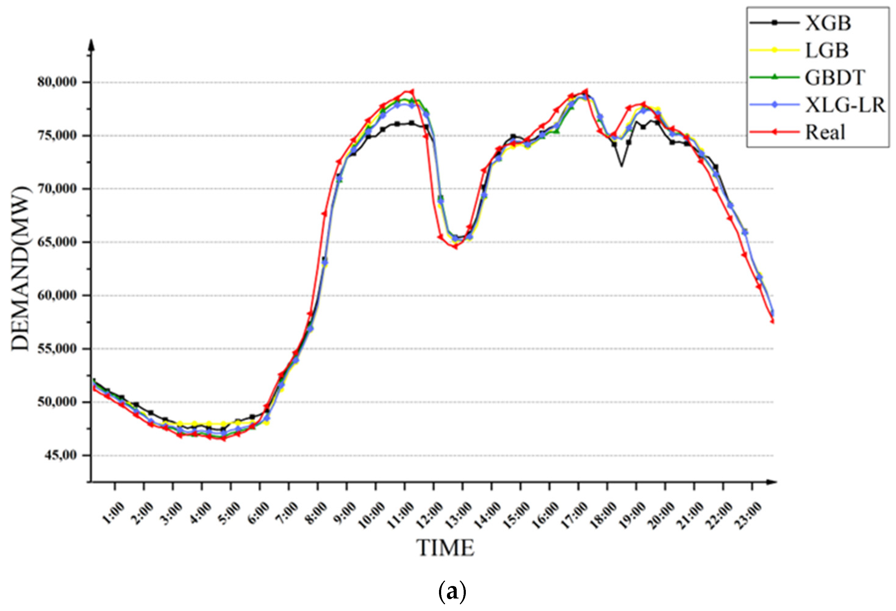
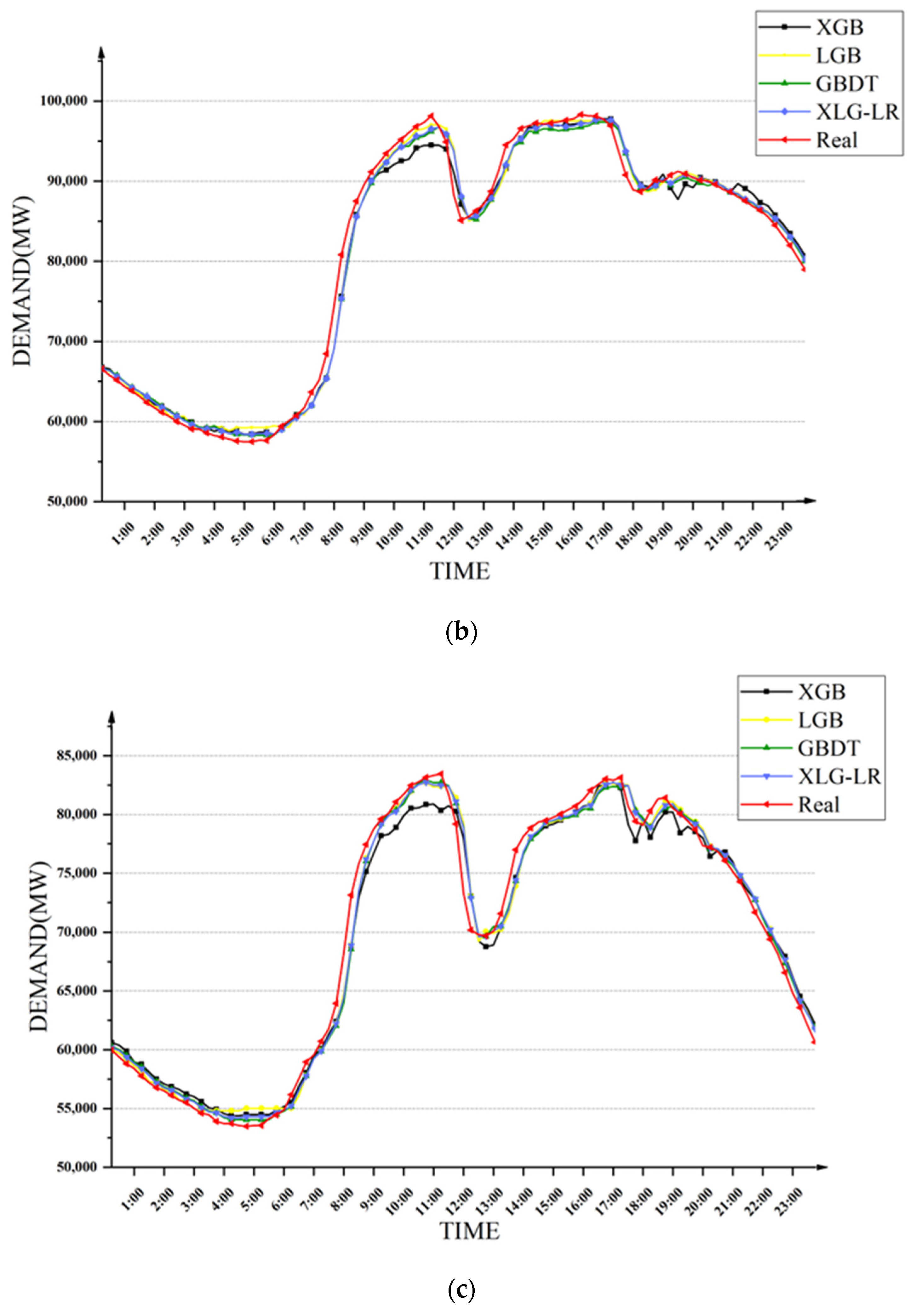
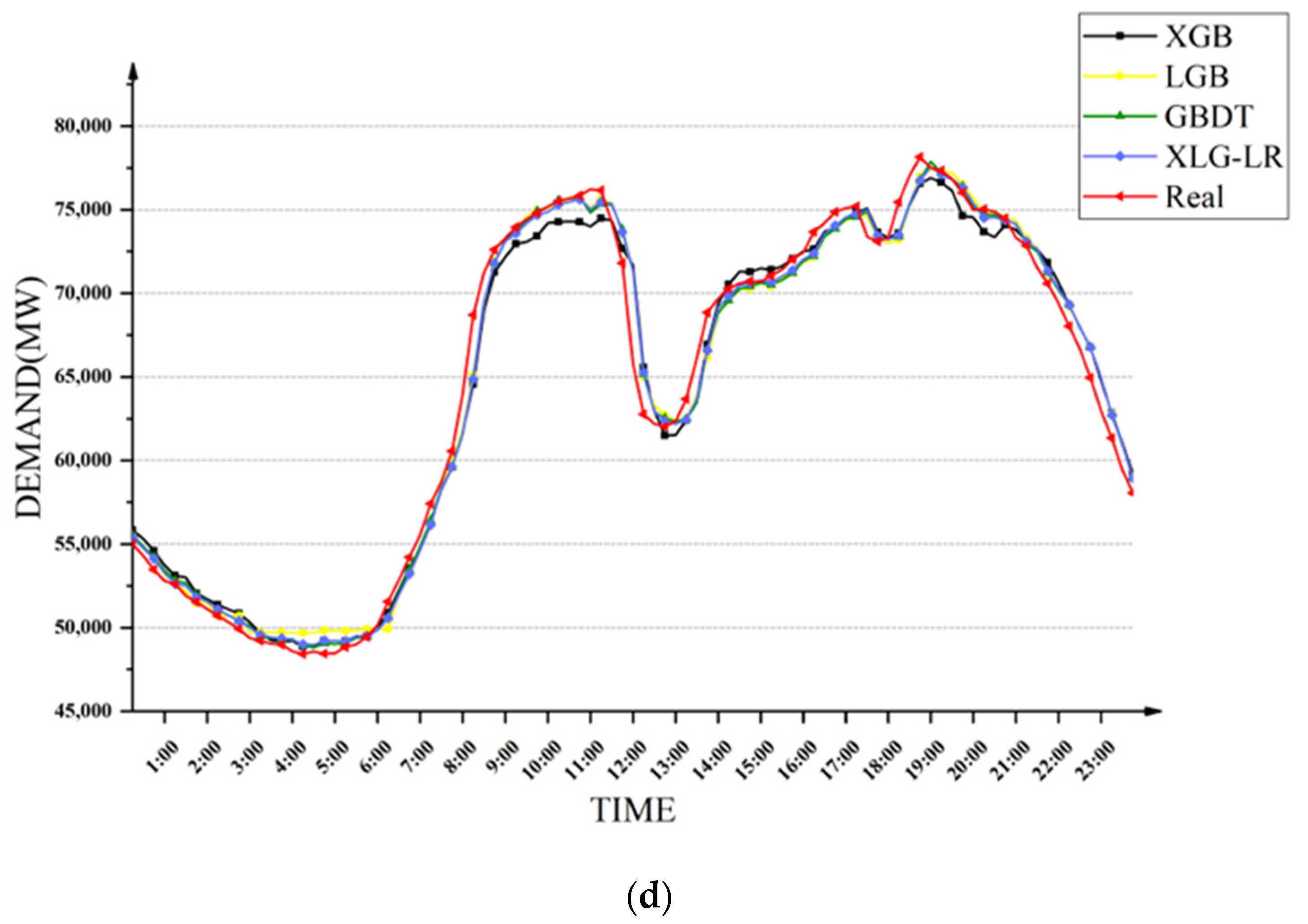
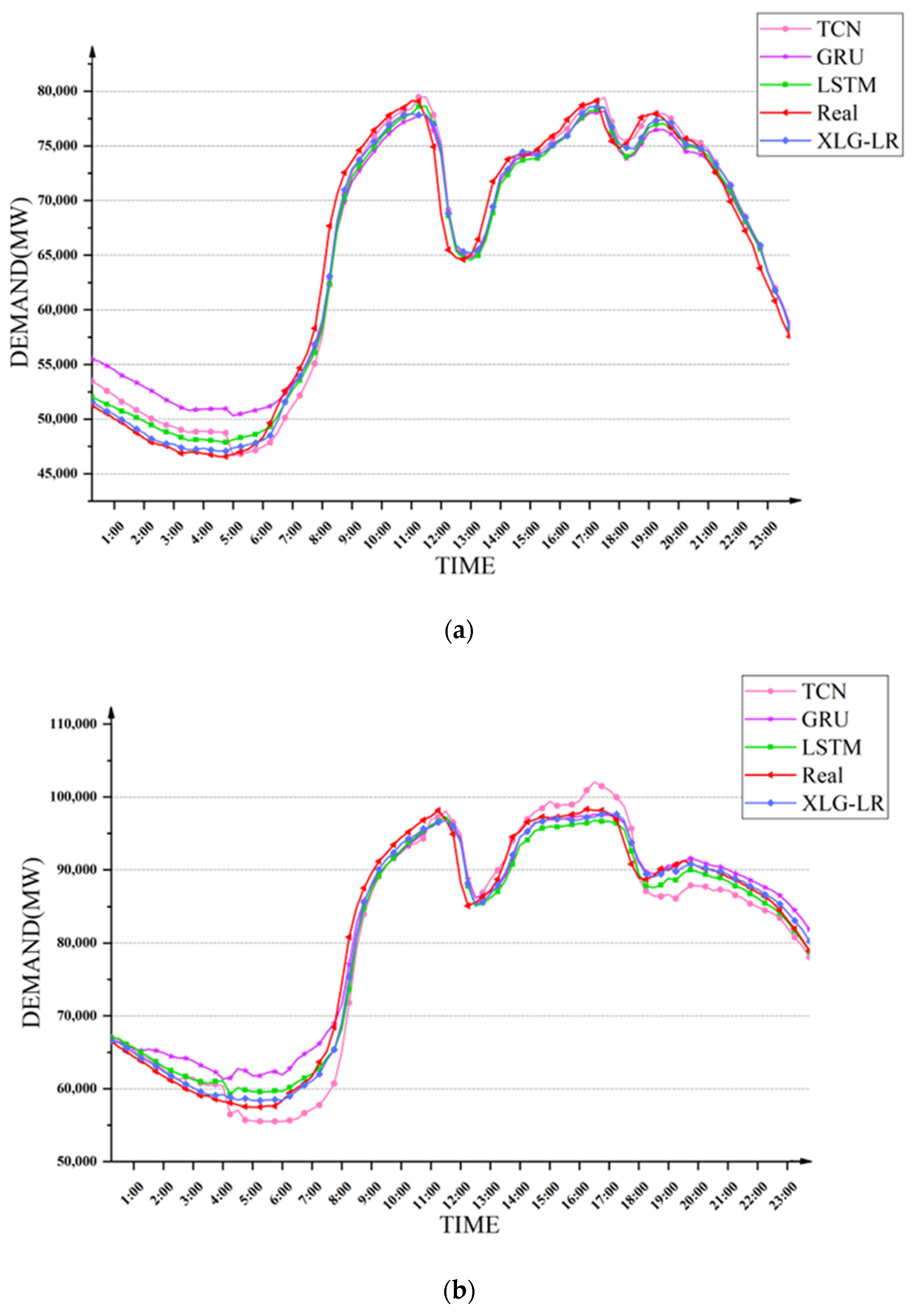
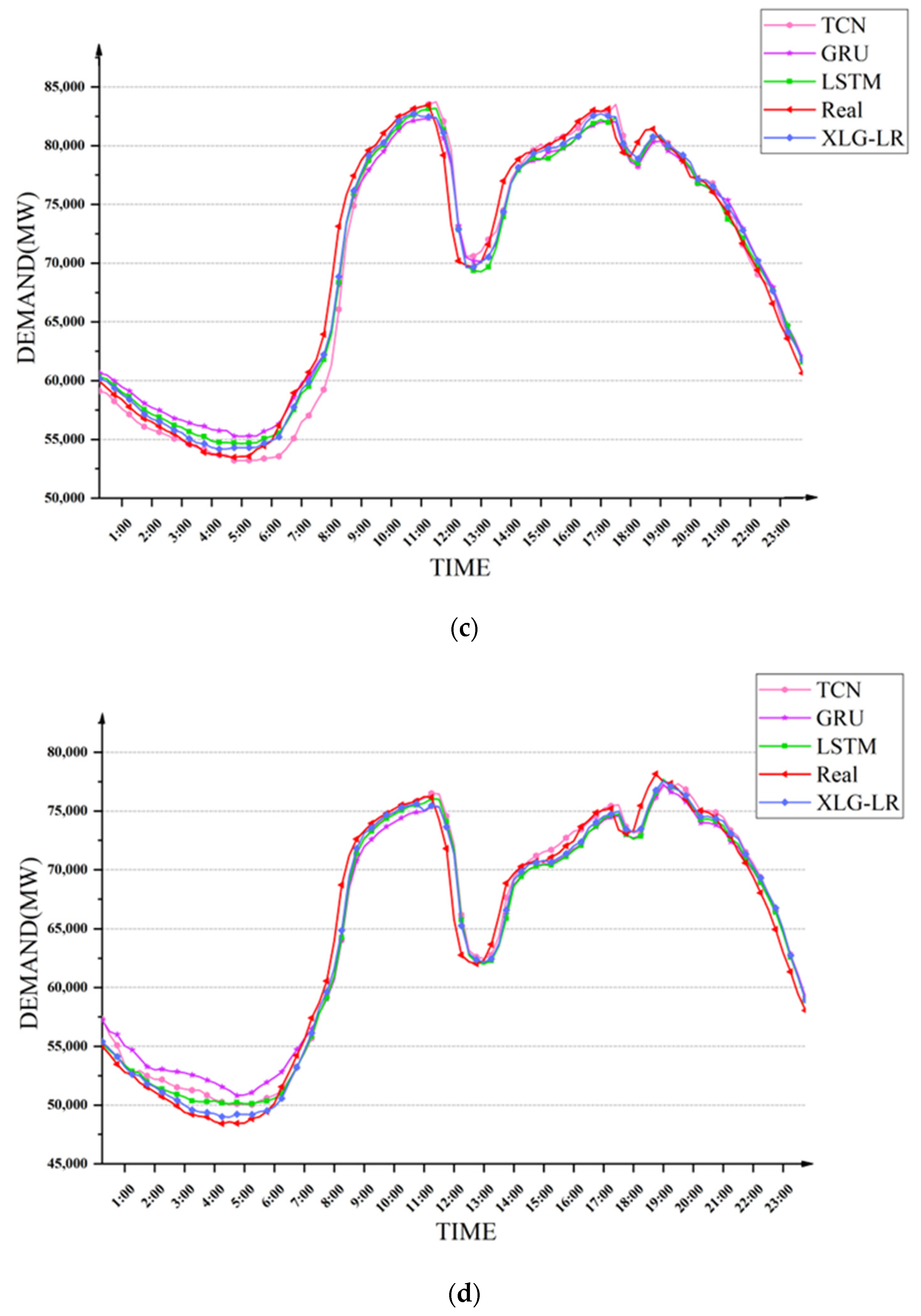
First, four methods were used to compare the seasonal power demand forecasting, and the same training set and test set as Section 5.2 were utilized to carry out experiments to investigate the accuracy of power demand forecasting in different periods of a day in a certain season. The prediction results of the four models for different seasons of electricity demand are shown in Figure 10. It can be seen that the XLG-LR model was the closest to the true value in most time periods.

The comparison between the XLG-LR model in this paper and the other three neural network methods is shown in

Table 7. Four-season Power Demand Forecasting of Different Models.

Season	Model	MAE	RMSE	MAPE	${\mathit{R}}^2$
Spring	TCN	1391.5866	1821.2366	2.3494	0.9769
	GRU	2005.0183	2518.0632	3.5355	0.9558
	LSTM	1269.7824	1574.1374	2.0255	0.9827
	XLG-LR	944.2574	1324.2092	1.4290	0.9878
Summer	TCN	2337.1998	2953.7105	2.9954	0.9604
	GRU	1968.0719	2443.3270	2.78523	0.9729
	LSTM	1568.0717	1944.5349	2.0158	0.9828
	XLG-LR	1012.3726	1476.2730	1.2631	0.9901
Autumn	TCN	1131.3771	1849.1958	1.6581	0.9698
	GRU	1262.4749	1529.5060	1.8689	0.9794
	LSTM	1059.8789	1393.1455	1.5416	0.9829
	XLG-LR	849.6115	1212.4954	1.2145	0.9870
Winter	TCN	1159.8787	1520.9946	1.9049	0.9777
	GRU	1521.1682	1856.1513	2.5641	0.9668
	LSTM	1058.4183	1397.4117	1.6953	0.9812
	XLG-LR	820.0982	1165.8157	1.2753	0.9869

. It can be seen that compared with the three models of GRU, LSTM and TCN, the XLG-LR model has significant advantages in forecasting power demand in different seasons under the four evaluation indicators.

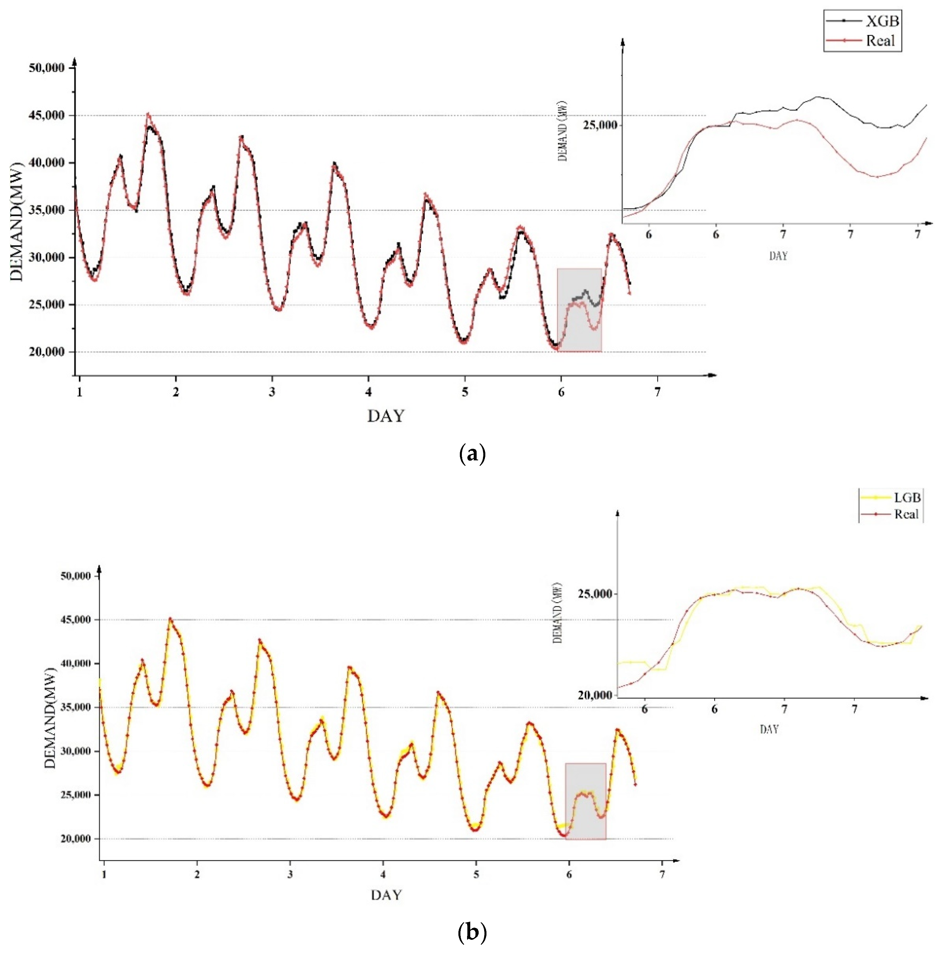
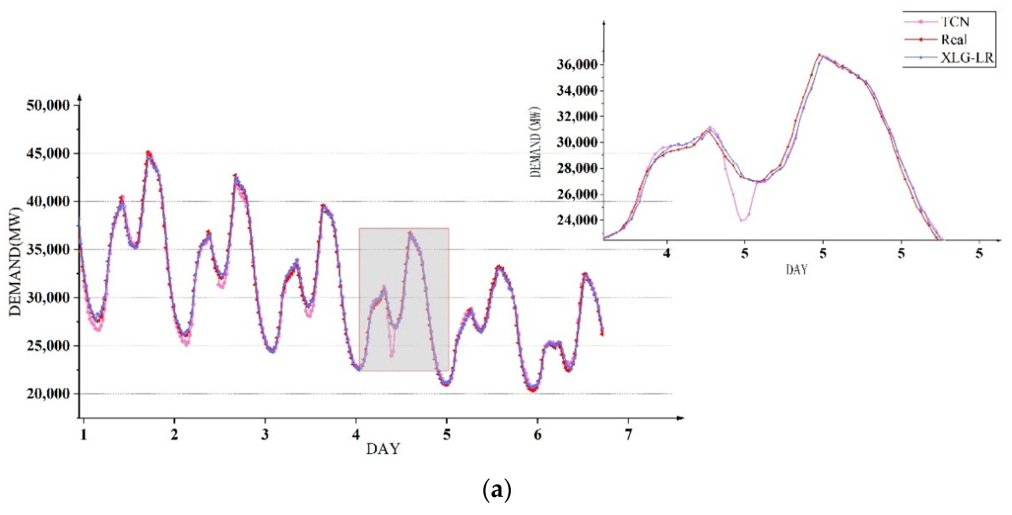
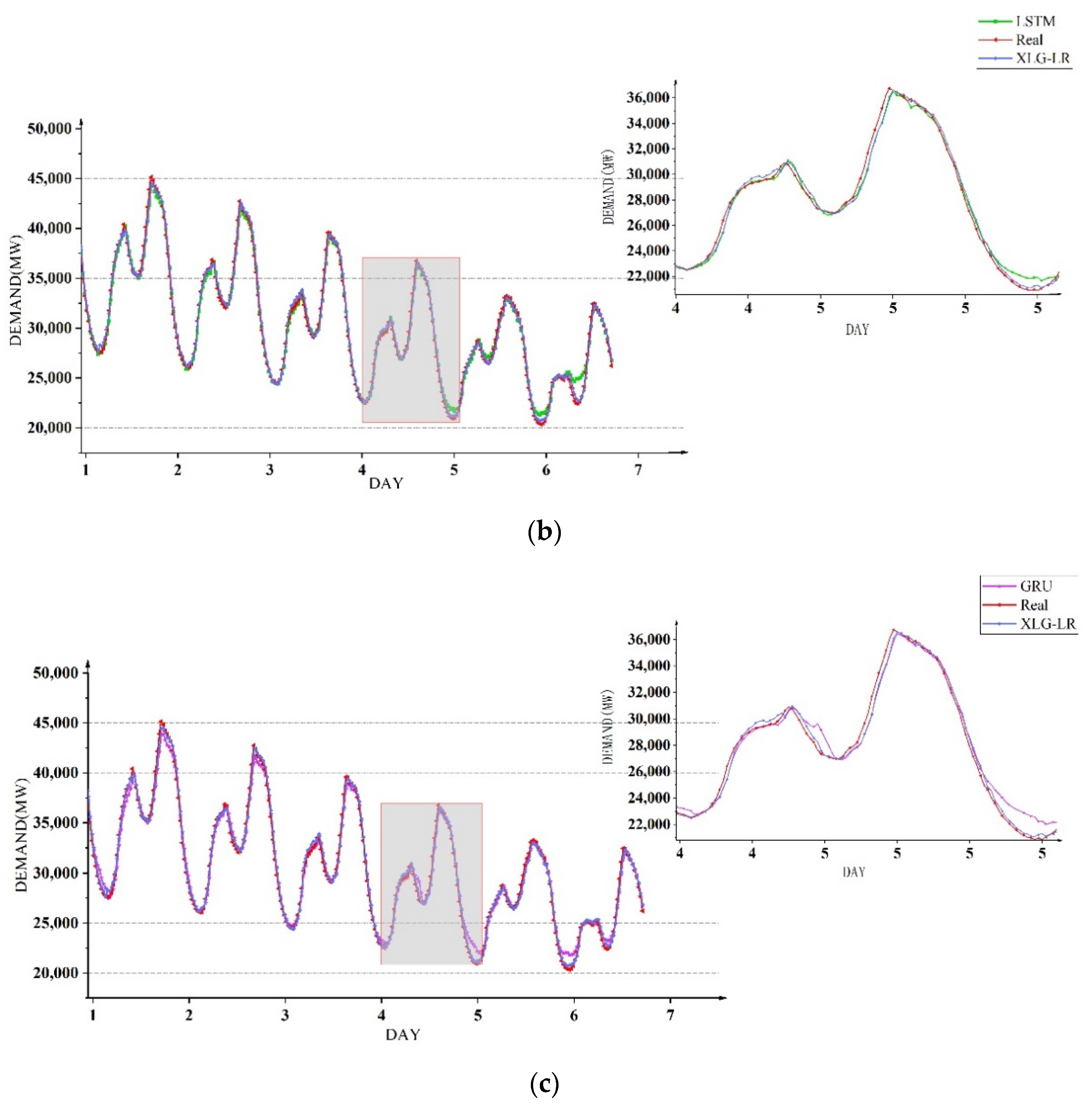
Secondly, four methods were used to compare power demand forecasting in weeks, and the same training set and test set as in Section 5.3 were utilized to conduct experiments to examine the accuracy of power demand forecasting at different time periods in a week. The prediction results of the four models for the trend of electricity demand in one week are shown in Figure 11. It can be seen that the three models GRU, LSTM and TCN had obvious prediction deviations in the periods of high and low electricity demand, while the XLG-LR model could accurately predict the change trend of power demand in most time periods.

The comparison between the XLG-LR model and the other three neural network methods are shown in

Table 8. Power Demand Forecasting of Different Models on a Weekly Basis.

Model	MAE	RMSE	MAPE	${\mathit{R}}^2$
TCN	458.1456	611.5984	1.5005	0.9908
GRU	546.6451	697.3183	1.7744	0.9881
LSTM	442.0174	605.2217	1.4582	0.9910
XLG-LR	383.7544	494.0599	1.2118	0.9940

. It can be seen that compared with the three models of GRU, LSTM and TCN, the XLG-LR model had obvious advantages in the power demand forecasting on a weekly basis under the four evaluation indicators, and all indicators were ahead of other models.

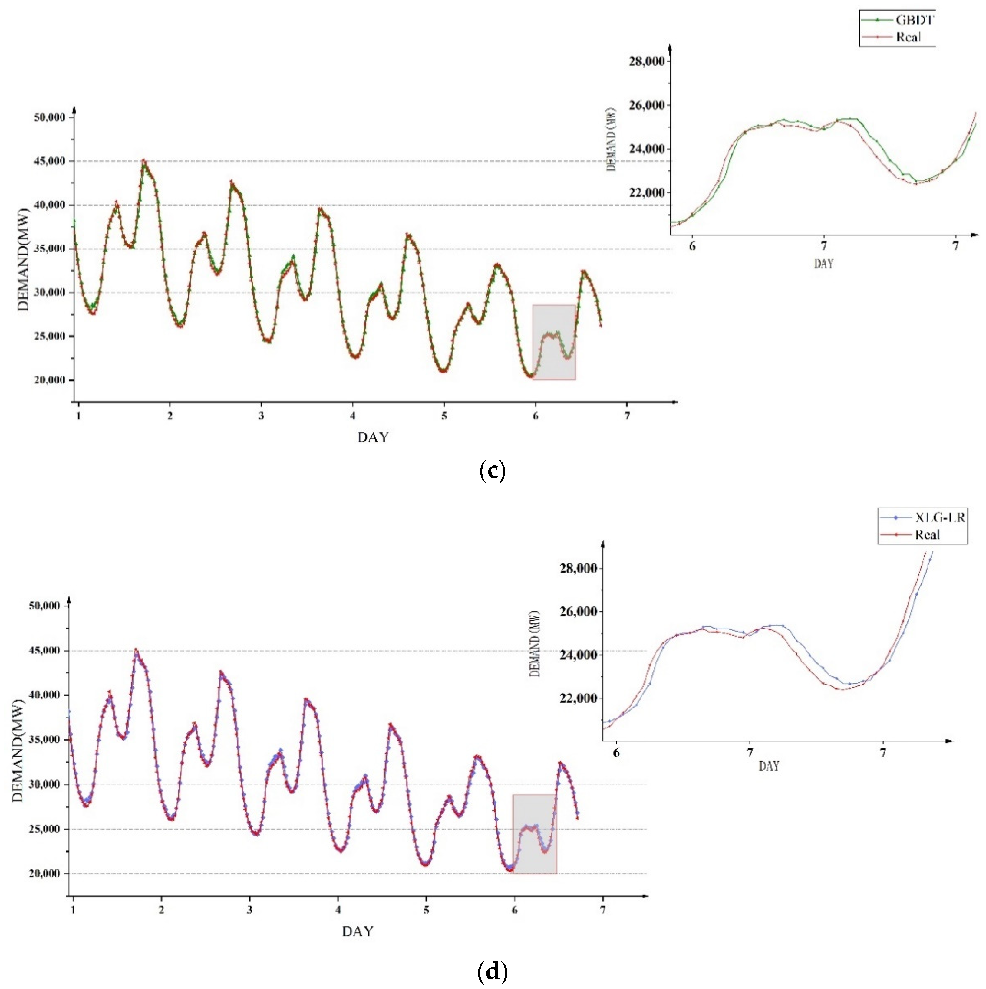
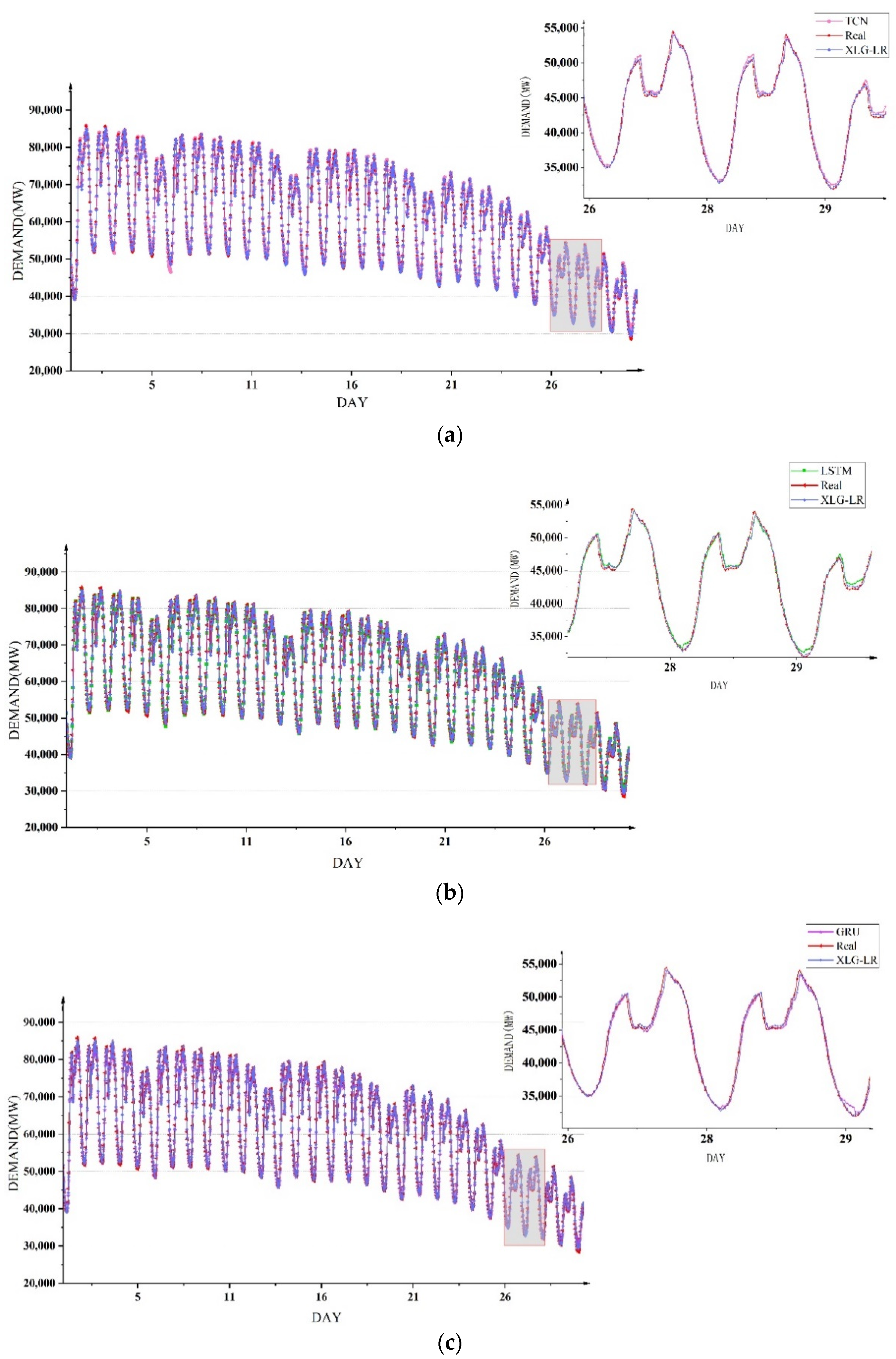
Then four methods were used to compare the power demand forecasting on a monthly basis, and the same training set and test set as Section 5.3 were utilized to conduct experiments to examine the accuracy of power demand forecasting at different time periods during the 30 days. Figure 12 shows the forecast results of the four models for the trend of electricity demand in one month. It can be seen from the figure that the three models of GRU, LSTM and TCN had obvious forecast deviations in the period of low electricity demand, while the XLG-LR model could basically match the real demand in most time periods.

The comparison between the XLG-LR model and the other three neural network methods are shown in

Table 9. Comparison of Power Demand Forecasting of Different Models on a Monthly Basis.

Model	MAE	RMSE	MAPE	${\mathit{R}}^2$
TCN	807.7706	1212.6045	1.4354	0.9928
GRU	820.3134	1222.5821	1.3882	0.9927
LSTM	811.6063	1217.4424	1.4310	0.9928
XLG-LR	700.9373	1032.5632	1.1818	0.9948

. It can be seen that compared with the three models of GRU, LSTM and TCN, the XLG-LR model had significant advantages in forecasting electricity demand on a monthly basis under the four evaluation indicators, and the curve fitting effect was the best and the power demand forecast error was the smallest.

The prediction time of the model was related to the convenience of the model in reality. This paper adopted the same training data to compare the time consumption of the XLG-LR model and the other three neural network methods in the prediction stage. The specific structure is shown in

Table 10. The Time Required for Power Demand Forecasting of Different Models in Different Scenarios.

Forecasting Scenario		Model	Predict Time(s)
Short-term power demand forecasting in different seasons	Spring	TCN	0.0745
		GRU	0.0587
		LSTM	0.0630
		XLG-LR	0.0018
	Summer	TCN	0.4250
		GRU	0.0629
		LSTM	0.0610
		XLG-LR	0.0016
	Autumn	TCN	0.0646
		GRU	0.0622
		LSTM	0.0626
		XLG-LR	0.0019
	Winter	TCN	0.0665
		GRU	0.0579
		LSTM	0.0616
		XLG-LR	0.0022
Power demand forecasting on a weekly basis		TCN	0.1432
		GRU	0.1042
		LSTM	0.1080
		XLG-LR	0.0026
Power demand forecasting on a monthly basis		TCN	0.4341
		GRU	0.2859
		LSTM	0.2748
		XLG-LR	0.0041

.

It can be seen from the table that the XLG-LR model could complete the prediction in the shortest time in each forecasting scenario. And the time required was at least one order of magnitude different than the other three neural network methods, which fully showed that the XLG-LR model had an absolute advantage in prediction time.

Through the above comparative experiments, it could be considered that the XLG-LR model had obvious advantages in terms of prediction accuracy and prediction time consumption compared with the classical neural network algorithms. The construction of the XLG-LR model mainly relies on the principle of a decision tree, and the global optimal solution is finally obtained by continuously optimizing the local optimal solution in the solving process. The neural network needs to compare the data features extracted from the test data with the trained model to give the optimal solution. However, the data in the training model has numerous features as well as a certain similarity, so it performs not as well as the XLG-LR model in terms of accuracy and time consumption. Therefore, it can be considered that the XLG-LR model in this study could achieve ideal prediction results for the power demand forecasting in different scenarios.

Although the method proposed in this paper has achieved relatively ideal power demand forecasting results, there are still some problems that need to be solved in the future.

(1) The dataset is relatively small and contains a limited amount of information. At present, the dataset used in this paper has only 13 months of data, which reduces the generalization and reliability of the model to a certain extent. The GBDT, XGBoost and LightGBM algorithms used in this paper can achieve better prediction results on small data sets, but if the data is more abundant, it should be able to achieve better prediction results. Therefore, in future research and exploration, the current dataset can be supplemented by collecting more months of data to build a larger and more informative dataset for electricity demand forecasting.

(2) More indicators other than meteorological factors may also be able to influence the forecast results. The electricity demand can be affected by many factors, including the level of local economic development and industrial structure. Although the indicators used in this study can exert the necessary influences on electricity demand to a certain extent, some other indicators may also affect it. Therefore, in the future, researchers can learn of other factors affecting electricity demand indicators from experts in related fields, and collect more index data that can have an impact on electricity demand to supplement the current data set.

7. Conclusions

Regarded as an important task in the power industry, power demand forecasting guarantees normal operation of economic development, sustains people’s daily life, and directs electric power production. This study utilized 13 months of electricity and meteorological data and adopted three models: GBDT, XGBoost and LightGBM, in order to build an XLG-LR power demand forecasting model based on stacking fusion. After the data was divided into a training set and a test set, the above four models were trained, and the test set was used to verify the feasibility of the model. The experiments in this study were carried out under the following software and hardware conditions. Software conditions required python3.7, tensorflow2.8.0, with the sklearn, seaborn, numpy, matplotlib, and the pandas development kits installed. The hardware environment required that the graphics card model was AMD Radeon(TM) Vega 8 Graphics and that the memory was 8 GB.

Verification started with different time lengths such as seasonal forecasting, weekly forecasting and monthly forecasting. It was found that under different time lengths, except for the XGBoost model, the GBDT, LightGBM and XLG-LR models all achieved relatively satisfactory results, among which the XLG-LR model proposed in this paper works best. From the perspective of prediction accuracy, the overall prediction accuracy ranked as XLG-LR > GBDT > LightGBM > XGBoost. In addition, this paper also compared the power demand prediction results of the XLG-LR model with that of the three mainstream neural network models of TCN, GRU and LSTM. The results showed that the XLG-LR model in this paper can also achieve the best experimental results in this dataset compared to the neural network model. Through the above discussion, the reliability and validity of the XLG-LR model in this paper for power demand forecasting was verified. When the power demand data or the meteorological data changes, only a new data set is needed to train the model to form a new prediction model, which can cope with the data changes and carry out the corresponding prediction. The method in this study can also be applied to power demand forecasting in other regions, and a new data set is needed to train a new forecasting model. In addition, the method has been encapsulated into corresponding software with good interoperability. It will be able to be used in a wider range of practical applications in the days to come.

In the future, more power demand data can be collected to build a larger power demand database so as to verify the accuracy and advancement of the algorithm in this paper in power demand forecasting. At the same time, under the premise that the amount of data is sufficient enough, this method could be adopted to carry out long-term electricity demand forecasting, such as forecasting the electricity demand in the next year. In addition, electricity demand is also closely related to other factors besides meteorological ones, such as the level of economic development and the regional industrial layout. In the days to come, these data can be supplemented to improve the prediction accuracy of this method. Furthermore, the method can also be applied to other fields, including the prediction of water demand and coal resource demand.