Global Prescribed-Time Stabilization of High-Order Nonlinear Systems with Asymmetric Actuator Dead-Zone

Abstract

This paper is concerned with the global prescribed-time stabilization problem for a class of uncertain high-order nonlinear systems (HONSs) with an asymmetric actuator dead-zone. Firstly, a new state-scaling transformation (SST) is developed for high-order nonlinear systems to change the original prescribed-time stabilization into the finite-time stabilization of the transformed one. The defects of the conventional one introduced in Song et al. (2017), which is unable to ensure the closed-loop stability behind a prespecified convergence time and a closed-loop system, which is only driven to the neighborhood of destination, is successfully overcome by introducing a switching mechanism in our proposed SST. Then, by using the adding a power integrator (API) technique, a state feedback controller is explicitly constructed to achieve the requirements of the closed-loop prescribed time convergence. Lastly, a liquid-level system is utilized to validate the theoretical results.

1. Introduction

During the past few years, high-order nonlinear systems (HONSs) have received a great deal of attention due to their significant value both in theory and practice [1,2]. However, the Jacobian linearization of HONSs is neither controllable nor feedback linearized, and feedback stabilization of such systems has been recognized as meaningful and challenging work. Fortunately, with the help of an added power integrator (API) [3] technique, many significant results have been produced regarding the asymptotic stabilizing/tracking control of HONSs; for examples, see [4,5,6,7] and references therein.

On the other hand, in recent years, the research on finite-time control has become a hot research area due to the finite-time stable system performing superior properties, such as both fast response and good disturbance rejection. Since the groundbreaking work in which the Lyapunov finite-time stability of nonlinear systems was introduced in [8], lots of important results have been established [9,10,11,12,13,14,15,16,17]. However, it should be pointed out that the above-mentioned results are subject to the issue that settling time functions is seriously dependent on initial system conditions, which causes their convergence time to experience unacceptably large increases as the magnitude of the initial conditions grows. To address this faultiness, the idea of fixed-time stability, which requires the upper boundedness of the involved settling time function be independent of initial system conditions, is put forward in [18]. So, under this new framework, many works have appeared to address fixed-time control of linear/nonlinear systems. Generally speaking, there are two kinds of existing design methods of fixed-time control: the bi-limit homogeneous-based method [18,19] and the Lyapunov-based method [20,21,22,23,24,25,26,27,28]. It should be mentioned that both methods suffer from some inherent shortcomings. In the former, the upper bound of the settling time (UBST) function exists, but it is usually unknown, and in the latter, the UBST is bounded and adjustable, but it is difficult or even impossible to prespecify discretionarily in the light of requirements because the derived settling time function relies on design parameters, whose choice is laborious when satisfying a pregiven settling time.

In fact, a prespecifiable settling time is desirable in many practical applications, e.g., missile guidance [29]. As a result, prescribed/predefined-time control has become an active research topic [30,31,32,33,34,35]. In particular, research has explored scaling the states using a function that increases unboundedly, trending towards the terminal time, a state-scaling design method to address the prescribed-time stabilization (PTS) of Brunovsky systems in [30]. By employing a switching mechanism to address the computationally singular aspect of the proposed controller, this technique was further extended to study the PTS of planar linear systems in [35]. However, only the linear case is studied in [35], which implies the proposed technique has difficulty handling strongly nonlinear systems, e.g., high-order nonlinear systems (HONSs) which are intrinsically nonlinear systems. This describes many practical systems [1]. Moreover, another common drawback of the aforementioned results is that the effect of the actuator dead-zone is ignored. Nevertheless, owing to physical limitations of device, many actual systems are usually inevitably subjected to input dead-zone nonlinearity during operation. Such undesirable property may significantly degrade the system’s performance or even system damage [36,37,38,39,40,41,42]. Therefore, an interesting question naturally arises: For HONSs with actuator dead-zone, is it possible to devise a controller to achieve the PTS? If possible, how can one design it? This paper focuses on addressing the problem of global PTS for a kind of HONSs with asymmetric actuator dead-zone and giving an affirmative answer to the above question. The significant contributions are underlined as follows.

(i)

Different from finite-time convergence in [41] or fixed-time convergence in [42], fully taking into consideration of practical system requirements, both asymmetric actuator dead-zone and prescribed-time convergence are included to study the stabilization problem of HONSs.

(ii)

To effectively overcome the computationally singular problem of the conventional scaling function-based design in [30], a novel switched scaling function with the switching rule involving both state and time is introduced.

(iii)

Under some weaker restricted conditions on characterizing system nonlinearities, a systematic design method is proposed by delicately utilizing the API technique to ensure the achievement of the performance requirements.

Notations. In this paper, the used notations are standard. Specifically, for a vector $x={(x_1,\dots ,x_n)}^T\in {\mathbb{R}}^n$, denote ${\overline{x}}_s=(x_1,$$\dots ,x_s{)}^T\in {\mathbb{R}}^s$, $s=1,\dots ,n$, and the function ${\lceil x\rceil }^c$ is defined as ${\lceil x\rceil }^c=\mathrm{sign}\left(x\right){\left|x\right|}^c$, with $\mathrm{sign}(·)$ being the signum function.

2. Problem Formulation and Preliminaries

2.1. Problem Formulation

Consider a kind of HONSs given by

$$\begin{array}{c}\hfill \left\{\begin{array}{c}{\dot{z}}_1=d_1\left(t\right){⌈z_2⌉}^{p_1}+f_1\left(z_1\right),\hfill \\ {\dot{z}}_2=d_2\left(t\right){⌈z_3⌉}^{p_2}+f_2\left({\overline{z}}_2\right),\hfill \\ ⋮\hfill \\ {\dot{z}}_{n-1}=d_{n-1}\left(t\right){⌈z_n⌉}^{p_{n-1}}+f_{n-1}\left({\overline{z}}_{n-1}\right),\hfill \\ {\dot{z}}_n=d_n\left(t\right)D\left(u\right)+f_n\left({\overline{z}}_n\right),\hfill \end{array}\right.\end{array}$$

(1)

where ${\overline{z}}_i=(z_1,$$\dots ,z_i{)}^T\in {\mathbb{R}}^i$ is the system state (vector), and $d_i\in \mathbb{R}$, $p_i\in {\mathbb{R}}^{+}$ (with $p_n=1$), $i=1,\dots ,n$ are the control coefficients and the power orders of the system, respectively. $f_i:{\mathbb{R}}^i\to \mathbb{R}$, $i=1,\dots ,n$ are uncertain continuous functions satisfying $f_i\left(0\right)=0$. $u\in \mathbb{R}$ is the real control input, and $D\in \mathbb{R}$ denotes the asymmetric actuator dead-zone which can be modeled as

$$D\left(u\right)=\left\{\begin{array}{ccc}{m}_r\left(t\right)(u-b_r\left(t\right)),\hfill & & u\ge b_r\left(t\right),\\ 0,\hfill & & -b_l\left(t\right)<u<b_r\left(t\right),\\ m_l\left(t\right)(u+b_l\left(t\right)),\hfill & & u\le -b_l\left(t\right),\end{array}\right.$$

(2)

where $m_r\left(t\right)$, $m_l\left(t\right)$ and $b_r\left(t\right)$, $b_l\left(t\right)$ are the corresponding the slopes and the breakpoints of the dead-zone characteristic, respectively.

The aim of this paper is to find a state feedback control mechanism which stabilizes system (1) within prescribed finite time under the following wild assumptions.

Assumption 1.

For $i=1,\dots ,n$, there are smooth functions ${\phi }_i\ge 0$ and a constant $\tau >0$ such that

$$\begin{array}{c}{\displaystyle |f_i\left({\overline{z}}_i\right)|\le {\phi }_i\left({\overline{z}}_i\right)\sum _{j=1}^i{\left|z_j\right|}^{\frac{{\lambda }_i-\tau }{{\lambda }_j}},}\hfill \end{array}$$

(3)

where ${\lambda }_i$s are recursively defined by

$$\begin{array}{c}{\lambda }_{n+1}=\tau ,p_i{\lambda }_{i+1}={\lambda }_i-\tau \ge 0,i=1,\dots ,n-1.\hfill \end{array}$$

(4)

Assumption 2.

There are positive constants ${\underline{d}}_i$ and ${\overline{d}}_i$, $i=1,\dots ,n$ such that ${\underline{d}}_i\le d_i\left(t\right)\le {\overline{d}}_i$.

Assumption 3.

There are positive constants ${\underline{m}}_r$, ${\underline{m}}_l$, ${\overline{b}}_r$ and ${\overline{b}}_l$, such that

$${\underline{m}}_r\le m_r\left(t\right),{\underline{m}}_l\le m_l\left(t\right),b_r\left(t\right)\le {\overline{b}}_r,b_l\left(t\right)\le {\overline{b}}_l.$$

(5)

Remark 1.

Assumption A1 can be regarded as a new growth-like condition where ${\lambda }_i$s are different from the traditional ones [4,5,6,7] where they are recursively given by ${\lambda }_1=1,p_i{\lambda }_{i+1}={\lambda }_i-\tau \ge 0,i=1,\dots ,n$. In addition, it should be mentioned that it is reasonable in engineering practice to impose the control coefficients and the unknown dead-zone parameters (i.e., the slopes and breakpoints) bounded in Assumptions 2 and 3. Similar requirements can be found in the existing literature [40,41].

2.2. Preliminaries

Consider the nonlinear system

$$\begin{array}{c}\dot{z}=f(t,z),z\left(0\right)=z_0\in {\mathbb{R}}^n,\hfill \end{array}$$

(6)

where $f:\mathbb{R}\times {\mathbb{R}}^n\to {\mathbb{R}}^n$ is continuous with respect to x and satisfies $f(t,0)=0$.

Definition 1

([8]). The origin of system (6) is said to be globally finite-time stable if it is globally asymptotically stable and for any $z_0\in {\mathbb{R}}^n$, a settling time function $T:{\mathbb{R}}^n\backslash \left\{0\right\}\to (0,+\infty )$ exists to ensure all solutions $z(t,z_0)$ of (6) satisfying $z(t,z_0)=0$, $\forall t\ge T\left(z_0\right)$.

Definition 2

([20]). The origin of system (6) is said to be globally fixed-time stable if it is globally finite-time stable and its settling-time function $T\left(z_0\right)$ is bounded by a positive constant; that is to say, $\exists T_{max}>0$, s.t. $T\left(z_0\right)\le T_{max}$, $\forall z_0\in {\mathbb{R}}^n$.

Definition 3

([32]). The origin of system (6) is said to be globally prescribed-time stable if it is globally fixed-time stable and for any prescribed time $T_p>0$, a tunable designing parameter $\theta \in \mathbb{R}$ exists to ensure $T\left(z_0\right)\le T_p$, $\forall z_0\in \mathbb{R}$.

Lemma 1

([8]). For system (6), if there is a $C^1$ and positive definite function $V\left(z\right)$ and some real numbers $c>0$ and $0<\alpha <1$ such that

$$\dot{V}\left(z\right)\le -c{V}^{\alpha }\left(z\right),\forall z\in {\mathbb{R}}^n.$$

Then, the origin of system (6) is finite-time stable with

$$T\left(z_0\right)\le \frac{V^{1-\alpha }\left(0\right)}{c(1-\alpha )},\forall z\in {\mathbb{R}}^n$$

Lemma 2

([3]). For any $u\in \mathbb{R}$, $v\in \mathbb{R}$, and a constant $m\ge 1$, one has (i) ${|u+v|}^m\le 2^{m-1}|u^m+v^m|$; (ii) $\left(\right|u|+{\left|v\right|)}^{1/m}\le {\left|u\right|}^{1/m}+{\left|v\right|}^{1/m}\le 2^{(m-1)/m}\left(\right|u|+{\left|v\right|)}^{1/m}$.

Lemma 3

([3]). For any constants $c,d>0$ and real-valued function $\delta (u,v)>0$, one has ${\left|u\right|}^c{\left|v\right|}^d\le \frac{c}{c+d}{\delta (u,v)\left|u\right|}^{c+d}+\frac{d}{c+d}{\delta }^{-c/d}(u,v){\left|v\right|}^{c+d}$.

Lemma 4

([4,43]). For any $u,v\in \mathbb{R}$ and constants $0<m\le 1$ and $b>0$, then, one has ${|\lceil u\rceil }^{bm}-{\lceil v\rceil }^{bm}|\le 2^{1-m}{|{\lceil u\rceil }^b-{\lceil v\rceil }^b|}^m.$

3. Main Results

This section proposes a constructive switching design mechanism of a state feedback controller to stabilize system (1) within any prescribed finite time $T_p>0$.

3.1. Scaling Function

For the aim of this paper, the following switched scaling function is introduced.

$$ϝ=\left\{\begin{array}{ccc}{\displaystyle \mathsf{\Gamma },}\hfill & \hfill & z\in \{{\mathbb{R}}^n-\mathsf{\Xi }\}\&t<T_s,\hfill \\ {\displaystyle 1,}\hfill & \hfill & \mathrm{otherwise},\hfill \end{array}\right.$$

(7)

where $\mathsf{\Xi }$ is a small closed neighborhood of origin and

$${\displaystyle \mathsf{\Gamma }=\frac{T_s}{T_s-t},}$$

(8)

with the positive design parameter $T_s$ satisfying $0<T_s<T_p$.

Remark 2.

It is obvious that Γ monotonically increases on $[0,T_s)$ with $\mathsf{\Gamma }\left(0\right)=1$ and $\mathsf{\Gamma }\left(T_s\right)=+\infty$. To address the incapability of ensuring the closed-loop viability and stability behind $T_s$, a new switched scaling function (7) is introduced in this paper. In comparison with the one used in [30], its novelty is that the switching rule is dependent on both state and time, i.e., it uses a small closed neighborhood of origin Ξ to replace the origin, which renders the system trajectory $z\left(t\right)$ to the switching set Ξ at some moment before $T_s$ can effectively overcome the computationally singular problem ($\infty \times 0$ type) of the resulting controller as $t\to T_s$.

3.2. Controller Design

Based on the above switched scaling function, the following novel coordinate transformation is given.

$$\begin{array}{c}{\zeta }_i={ϝ}^{(1+c){\lambda }_i}{z}_i,i=1,\dots ,n,D\left(v\right)={ϝ}^{(1+c){\lambda }_{n+1}}D\left(u\right),\hfill \end{array}$$

(9)

where $c\ge (1/\tau )-1$ is a design constant.

With the aid of (9), system (1) is redescribed as

$$\begin{array}{c}\hfill \left\{\begin{array}{c}{\dot{\zeta }}_1={ϝ}^{(1+c)\tau }\left(d_1{⌈{\zeta }_2⌉}^{p_1}+F_1\left({\zeta }_1\right)\right),\hfill \\ {\dot{\zeta }}_2={ϝ}^{(1+c)\tau }\left(d_2{⌈{\zeta }_3⌉}^{p_2}+F_2\left({\overline{\zeta }}_2\right)\right),\hfill \\ ⋮\hfill \\ {\dot{\zeta }}_{n-1}={ϝ}^{(1+c)\tau }\left(d_{n-1}{⌈{\zeta }_n⌉}^{p_{n-1}}+F_{n-1}\left({\overline{\zeta }}_{n-1}\right)\right),\hfill \\ {\dot{\zeta }}_n={ϝ}^{(1+c)\tau }\left(d_{n}D\left(v\right)+F_n\left({\overline{\zeta }}_n\right)\right),\hfill \end{array}\right.\end{array}$$

(10)

where

$$\begin{array}{c}{\displaystyle F_i\left({\overline{\zeta }}_i\right)={\zeta }_i\frac{(1+c){\lambda }_i\dot{ϝ}}{{ϝ}^{1+(1+c)\tau }}+{ϝ}^{(1+c)({\lambda }_i-\tau )}{f}_i\left({\overline{z}}_i\right),i=1,\dots ,n,}\hfill \end{array}$$

(11)

for which there are the smooth functions ${\overline{\phi }}_i\left({\overline{\zeta }}_i\right)\ge 0$ such that

$$\begin{array}{c}{\displaystyle |F_i\left({\overline{\zeta }}_i\right)|\le {\overline{\phi }}_i\left({\overline{\zeta }}_i\right)\sum _{j=1}^i{\left|{\zeta }_j\right|}^{\frac{{\lambda }_i-\tau }{{\lambda }_j}},i=1,\dots ,n.}\hfill \end{array}$$

(12)

Next, a state feedback stabilizing controller of system (10) is designed by employing the API technique.

Step 1. Let $\rho \ge {max}_{1\le i\le n}\left\{{\lambda }_i\right\}$ being a constant and take the Lyapunov function $V_1$ as

$$\begin{array}{c}{\displaystyle V_1=W_1={\int }_0^{{\zeta }_1}{⌈{\lceil s\rceil }^{\frac{\rho }{{\lambda }_1}}-0⌉}^{\frac{2\rho -{\lambda }_1}{\rho }}ds.}\hfill \end{array}$$

(13)

Applying Assumptions 1 and 2 and (12) produces

$$\begin{array}{c}{\displaystyle {\dot{V}}_1={ϝ}^{(1+c)\tau }{\lceil {\pi }_1\rceil }^{\frac{2\rho -{\lambda }_1}{\rho }}\left(d_1{\lceil {\zeta }_2\rceil }^{p_1}+F_1\right)}\hfill \\ {\displaystyle \le {ϝ}^{(1+c)\tau }\left({\lceil {\pi }_1\rceil }^{\frac{2\rho -{\lambda }_1}{\rho }}{d}_1{({\zeta }_2\rceil }^{p_1}-{\lceil {\zeta }_2^{*}\rceil }^{p_1})+d_1{\lceil {\pi }_1\rceil }^{\frac{2\rho -{\lambda }_1}{\rho }}{\lceil {\zeta }_2^{*}\rceil }^{p_1}+{\left|{\pi }_1\right|}^{\frac{2\rho -{\lambda }_1}{\rho }}{\overline{\phi }}_1\right),}\hfill \end{array}$$

(14)

where ${\pi }_1={\lceil {\zeta }_1\rceil }^{\frac{\rho }{{\lambda }_1}}$ and ${\zeta }_2^{*}$ is the virtual controller of ${\zeta }_2$.

Take the virtual controller

$$\begin{array}{c}{\displaystyle {\zeta }_2^{*}=-{\lceil {\pi }_1\rceil }^{\frac{{\lambda }_2}{\rho }}{\beta }_1^{\frac{{\lambda }_2}{\rho }}\left({\zeta }_1\right),}\hfill \end{array}$$

(15)

where

$$\begin{array}{c}{\displaystyle {\beta }_1\left({\zeta }_1\right)\ge {\left(\frac{n+{\overline{\phi }}_1}{{\underline{d}}_1}\right)}^{\frac{\rho }{p_1{\lambda }_2}},}\hfill \end{array}$$

(16)

is a smooth function. Then, by substituting (15) and (16) into (14), we have

$$\begin{array}{c}{\displaystyle {\dot{V}}_1\le -n{ϝ}^{(1+c)\tau }{\left|{\pi }_1\right|}^{\frac{2\rho -\tau }{\rho }}+{ϝ}^{(1+c)\tau }{d}_1{\lceil {\pi }_1\rceil }^{\frac{2\rho -{\lambda }_1}{\rho }}\left({\lceil {\zeta }_2\rceil }^{p_1}-{\lceil {\zeta }_2^{*}\rceil }^{p_1}\right).}\hfill \end{array}$$

(17)

Step 2. Define ${\pi }_2={\lceil {\zeta }_2\rceil }^{\frac{\rho }{{\lambda }_2}}-{\lceil {\zeta }_2^{*}\rceil }^{\frac{\rho }{{\lambda }_2}}$ and take the Lyapunov function $V_2=V_1+W_2$ with

$$\begin{array}{c}{\displaystyle W_2={\int }_{{\zeta }_2^{*}}^{{\zeta }_2}{⌈{\lceil s\rceil }^{\frac{\rho }{{\lambda }_2}}-{\lceil {\zeta }_2^{*}\rceil }^{\frac{\rho }{{\lambda }_2}}⌉}^{\frac{2\rho -{\lambda }_2}{\rho }}ds.}\hfill \end{array}$$

(18)

From

$$\left\{\begin{array}{c}{\displaystyle \frac{\partial W_2}{\partial {\zeta }_2}={\lceil {\pi }_2\rceil }^{\frac{2\rho -{\lambda }_2}{\rho }},}\hfill \\ {\displaystyle \frac{\partial W_2}{\partial {\zeta }_1}=-\frac{2\rho -{\lambda }_2}{\rho }\frac{\partial \left({\lceil {\zeta }_2^{*}\rceil }^{\frac{\rho }{{\lambda }_2}}\right)}{\partial {\zeta }_1}\times {\int }_{{\zeta }_2^{*}}^{{\zeta }_2}{\left|{\lceil s\rceil }^{\frac{\rho }{{\lambda }_2}}-{⌈{\zeta }_2^{*}⌉}^{\frac{\rho }{{\lambda }_2}}\right|}^{\frac{\rho -{\lambda }_2}{\rho }}ds,}\hfill \end{array}\right.$$

(19)

a direct calculation gives

$$\begin{array}{ccc}{\displaystyle {\dot{V}}_2}\hfill & \le \hfill & -n{ϝ}^{(1+c)\tau }{\left|{\pi }_1\right|}^{\frac{2\rho -\tau }{\rho }}+{ϝ}^{(1+c)\tau }{d}_1{\lceil {\pi }_1\rceil }^{\frac{2\rho -{\lambda }_1}{\rho }}\left({\lceil {\zeta }_2\rceil }^{p_1}-{\lceil {\zeta }_2^{*}\rceil }^{p_1}\right)\hfill \\ \hfill & \hfill & {\displaystyle +\frac{\partial W_2}{\partial {\zeta }_1}{ϝ}^{(1+c)\tau }(d_1{\lceil {\zeta }_2\rceil }^{p_1}+F_1)+\frac{\partial W_2}{\partial {\zeta }_2}{ϝ}^{(1+c)\tau }(d_2{\lceil {\zeta }_3\rceil }^{p_2}+F_2)}\hfill \\ \hfill & \le \hfill & -n{ϝ}^{(1+c)\tau }{\left|{\pi }_1\right|}^{\frac{2\rho -\tau }{\rho }}+{ϝ}^{(1+c)\tau }{d}_1{\lceil {\pi }_1\rceil }^{\frac{2\rho -{\lambda }_1}{\rho }}\left({\lceil {\zeta }_2\rceil }^{p_1}-{\lceil {\zeta }_2^{*}\rceil }^{p_1}\right)\hfill \\ \hfill & \hfill & {\displaystyle +{ϝ}^{(1+c)\tau }\left(\frac{\partial W_2}{\partial {\zeta }_1}(d_1{\lceil {\zeta }_2\rceil }^{p_1}+F_1)+d_2{\lceil {\pi }_2\rceil }^{\frac{2\rho -{\lambda }_2}{\rho }}\left({\lceil {\zeta }_3\rceil }^{p_2}-{\lceil {\zeta }_3^{*}\rceil }^{p_2}\right)\right.}\hfill \\ \hfill & \hfill & \left.+d_2{\lceil {\pi }_2\rceil }^{\frac{2\rho -{\lambda }_2}{\rho }}{\lceil {\zeta }_3^{*}\rceil }^{p_2}+{\lceil {\pi }_2\rceil }^{\frac{2\rho -{\lambda }_2}{\rho }}{F}_2\right),\hfill \end{array}$$

(20)

where ${\zeta }_3^{*}$ is the virtual controller to be designed later. To continue, the following upper bound estimates for some terms of (20) are needed.

Firstly, from the definitions of ${\pi }_j$ and ${\zeta }_j^{*}$ ($j=1,2$) and Lemma 4, one has

$$\begin{array}{ccc}{\displaystyle \left|{\lceil {\zeta }_2\rceil }^{p_1}-{\lceil {\zeta }_2^{*}\rceil }^{p_1}\right|}\hfill & =\hfill & \left|{\left({\lceil {\zeta }_2\rceil }^{\frac{\rho }{{\lambda }_2}}\right)}^{\frac{{\lambda }_2{p}_1}{\rho }}-{\left({\lceil {\zeta }_2^{*}\rceil }^{\frac{\rho }{{\lambda }_2}}\right)}^{\frac{{\lambda }_2{p}_1}{\rho }}\right|\hfill \\ \hfill & \le \hfill & 2^{1-\frac{{\lambda }_2{p}_1}{\rho }}|{\lceil {\zeta }_2\rceil }^{\frac{\rho }{{\lambda }_2}}-{\lceil {\zeta }_2^{*}\rceil }^{\frac{\rho }{{\lambda }_2}}{|}^{\frac{{\lambda }_2{p}_1}{\rho }}\hfill \\ \hfill & =\hfill & 2^{1-\frac{{\lambda }_2{p}_1}{\rho }}{\left|{\pi }_2\right|}^{\frac{{\lambda }_2{p}_1}{\rho }}.\hfill \end{array}$$

(21)

Thus, from (22), Assumption A2 and Lemma 3, it is obtained that

$$\begin{array}{ccc}{\displaystyle d_1{\lceil {\pi }_1\rceil }^{\frac{2\rho -{\lambda }_1}{\rho }}\left({\lceil {\zeta }_2\rceil }^{p_1}-{\lceil {\zeta }_2^{*}\rceil }^{p_1}\right)}\hfill & \le \hfill & {\displaystyle 2^{1-\frac{{\lambda }_2{p}_1}{\rho }}{\overline{d}}_1|{\pi }_1{|}^{\frac{2\rho -{\lambda }_1}{\rho }}{\left|{\pi }_2\right|}^{\frac{{\lambda }_2{p}_1}{\rho }}}\hfill \\ \hfill & \le \hfill & {\displaystyle \frac{1}{3}|{\pi }_1{|}^{\frac{2\rho -\tau }{\rho }}+{\left|{\pi }_2\right|}^{\frac{2\rho -\tau }{\rho }}{\varrho }_{21},}\hfill \end{array}$$

(22)

where ${\varrho }_{21}\ge 0$ is a smooth function.

Secondly, from (12) and Lemma 2, one gets

$$\begin{array}{ccc}|F_2|\hfill & \le \hfill & {\displaystyle {\overline{\phi }}_2\left(|{\zeta }_1{|}^{\frac{{\lambda }_2-\tau }{{\lambda }_1}}+{\left|{\zeta }_2\right|}^{\frac{{\lambda }_2-\tau }{{\lambda }_2}}\right)}\hfill \\ \hfill & \le \hfill & {\displaystyle {\overline{\phi }}_2\left(|{\pi }_1{|}^{\frac{{\lambda }_2-\tau }{\rho }}+|{\pi }_2{|}^{\frac{{\lambda }_2-\tau }{\rho }}+{\beta }_1^{\frac{{\lambda }_2-\tau }{\rho }}{\left|{\pi }_1\right|}^{\frac{{\lambda }_2-\tau }{\rho }}\right)}\hfill \\ \hfill & \le \hfill & {\tilde{\phi }}_2\left(|{\pi }_1{|}^{\frac{{\lambda }_2-\tau }{\rho }}+{\left|{\pi }_2\right|}^{\frac{{\lambda }_2-\tau }{\rho }}\right),\hfill \end{array}$$

(23)

where ${\tilde{\phi }}_2\ge$ $\left(1+{\beta }_1^{\frac{{\lambda }_2-\tau }{\rho }}\right){\overline{\phi }}_2$ is a smooth function.

Using (23) and Lemma 3 yields

$$\begin{array}{ccc}{\displaystyle {\lceil {\pi }_2\rceil }^{\frac{2\rho -{\lambda }_2}{\rho }}{F}_2}\hfill & \le \hfill & {\displaystyle {\lceil {\pi }_2\rceil }^{\frac{2\rho -{\lambda }_2}{\rho }}{\tilde{\phi }}_2\left(|{\pi }_1{|}^{\frac{{\lambda }_2-\tau }{\rho }}+{\left|{\pi }_2\right|}^{\frac{{\lambda }_2-\tau }{\rho }}\right)}\hfill \\ \hfill & \le \hfill & {\displaystyle \frac{1}{3}|{\pi }_1{|}^{\frac{2\rho -\tau }{\rho }}+{\left|{\pi }_2\right|}^{\frac{2\rho -\tau }{\rho }}{\varrho }_{22},}\hfill \end{array}$$

(24)

where ${\varrho }_{22}\ge 0$ is a smooth function.

Finally, note that

$$\begin{array}{ccc}{\displaystyle \frac{2\rho -{\lambda }_2}{\rho }{\int }_{{\zeta }_2^{*}}^{{\zeta }_2}{\left|{\lceil s\rceil }^{\frac{\rho }{{\lambda }_2}}-{⌈{\zeta }_2^{*}⌉}^{{\frac{\rho }{\lambda }}_2}\right|}^{\frac{\rho -{\lambda }_2}{\rho }}ds}\hfill & \le \hfill & {\displaystyle \frac{2\rho -{\lambda }_2}{\rho }|{\pi }_2{|}^{\frac{\rho -{\lambda }_2}{\rho }}|{\zeta }_2-{\zeta }_2^{*}|}\hfill \\ \hfill & \le \hfill & {\displaystyle \frac{2\rho -{\lambda }_2}{\rho }{2}^{1-\frac{{\lambda }_2}{\rho }}\left|{\pi }_2\right|,}\hfill \end{array}$$

(25)

and

$$\begin{array}{ccc}{\displaystyle \left|\frac{\partial \left({\lceil {\zeta }_2^{*}\rceil }^{\frac{\rho }{{\lambda }_2}}\right)}{\partial {\zeta }_1}\right|}\hfill & =\hfill & {\displaystyle \left|\frac{\partial \left({\beta }_1\lceil {\pi }_1\rceil \right)}{\partial {\zeta }_1}\right|}\hfill \\ \hfill & \le \hfill & {\displaystyle \left|\frac{\partial {\beta }_1}{\partial {\zeta }_1}\right||{\pi }_1|+\frac{\rho }{{\lambda }_1}{\beta }_1{\left|{\pi }_1\right|}^{\frac{\rho -{\lambda }_1}{\rho }}}\hfill \\ \hfill & \le \hfill & |{\pi }_1{|}^{\frac{\rho -{\lambda }_1}{\rho }}{\gamma }_2,\hfill \end{array}$$

(26)

where ${\gamma }_2\ge 0$ is a smooth function.

Therefore, in the light of (23), (25), (26) and Lemma 3, one concludes that

$${\displaystyle \begin{array}{ccc}\hfill & \hfill & {\displaystyle \frac{\partial W_2}{\partial {\zeta }_1}(d_1{\lceil {\zeta }_2\rceil }^{p_1}+F_1)}\hfill \\ \hfill & \le \hfill & {\displaystyle \frac{2\rho -{\lambda }_2}{\rho }{\int }_{{\zeta }_2^{*}}^{{\zeta }_2}{\left|{\lceil s\rceil }^{\frac{\rho }{{\lambda }_2}}-{⌈{\zeta }_2^{*}⌉}^{\frac{\rho }{{\lambda }_2}}\right|}^{\frac{\rho -{\lambda }_2}{\rho }}ds\times \left|\frac{\partial \left({\lceil {\zeta }_2^{*}\rceil }^{{\frac{\rho }{\lambda }}_2}\right)}{\partial {\zeta }_1}\right|(d_1{\lceil {\zeta }_2\rceil }^{p_1}+F_1)}\hfill \\ \hfill & \le \hfill & \frac{1}{3}|{\pi }_1{|}^{\frac{2\rho -\tau }{\rho }}+{\left|{\pi }_2\right|}^{\frac{2\rho -\tau }{\rho }}{\varrho }_{23},\hfill \end{array}}$$

(27)

where ${\varrho }_{23}\ge 0$ is a smooth function.

Substituting (22), (24) and (27) into (21) yields

$$\begin{array}{ccc}{\displaystyle {\dot{V}}_2}\hfill & \le \hfill & -(n-1){ϝ}^{(1+c)\tau }{\left|{\pi }_1\right|}^{\frac{2\rho -\tau }{\rho }}+{ϝ}^{(1+c)\tau }{d}_2{\lceil {\pi }_2\rceil }^{\frac{2\rho -r_2}{\rho }}\left({\lceil {\zeta }_3\rceil }^{p_2}-{\lceil {\zeta }_3^{*}\rceil }^{p_2}\right)\hfill \\ \hfill & \hfill & +{ϝ}^{(1+c)\tau }\left(d_2{\lceil {\pi }_2\rceil }^{\frac{2\rho -r_2}{\rho }}{\lceil {\zeta }_3^{*}\rceil }^{p_2}+({\varrho }_{21}+{\varrho }_{22}+{\varrho }_{23}){\left|{\pi }_2\right|}^{\frac{2\rho -\tau }{\rho }}\right).\hfill \end{array}$$

(28)

Then, one can design the virtual controller

$$\begin{array}{c}{\zeta }_3^{*}=-{\lceil {\pi }_2\rceil }^{\frac{{\lambda }_3}{\rho }}{\beta }_2^{\frac{{\lambda }_3}{\rho }}\left({\overline{\zeta }}_2\right),\hfill \end{array}$$

(29)

where the smooth function ${\beta }_2$ satisfies

$$\begin{array}{c}{\displaystyle {\beta }_2\left({\overline{\zeta }}_2\right)\ge {\left(\frac{n-1+{\varrho }_{21}+{\varrho }_{22}+{\varrho }_{23}}{{\underline{d}}_2}\right)}^{\frac{\rho }{q_2{\lambda }_3}},}\hfill \end{array}$$

(30)

such that

$$\begin{array}{ccc}{\displaystyle {\dot{V}}_2}\hfill & \le \hfill & -(n-1){ϝ}^{(1+c)\tau }\left(|{\pi }_1{|}^{\frac{2\rho -\tau }{\rho }}+{\left|{\pi }_2\right|}^{\frac{2\rho -\tau }{\rho }}\right)+{ϝ}^{(1+c)\tau }{d}_2{\lceil {\pi }_2\rceil }^{\frac{2\rho -r_2}{\rho }}\left({\lceil {\zeta }_3\rceil }^{p_2}-{\lceil {\zeta }_3^{*}\rceil }^{p_2}\right).\hfill \end{array}$$

(31)

Following the same arguments of Step 2 for details, for Step i ( $i=2,\dots ,n$), we can find a $C^1$ and positive definite Lyapunov function $V_i={\sum }_{j=1}^i{W}_j$ with

$$\begin{array}{c}{\displaystyle W_i={\int }_{{\zeta }_i^{*}}^{{\zeta }_i}{⌈{\lceil s\rceil }^{\frac{\rho }{{\lambda }_i}}-{\lceil {\zeta }_i^{*}\rceil }^{\frac{\rho }{{\lambda }_i}}⌉}^{\frac{2\rho -{\lambda }_i}{\rho }}ds,}\hfill \end{array}$$

(32)

and a row of continuous virtual controllers ${\zeta }_{j+1}^{*}=-{\lceil {\pi }_j\rceil }^{\frac{{\lambda }_{j+1}}{\rho }}{\beta }_j^{\frac{{\lambda }_{j+1}}{\rho }}\left({\overline{\zeta }}_j\right)$, $j=1,\dots ,i$, such that

$$\begin{array}{c}{\displaystyle {\dot{V}}_i\le -(n-i+1){ϝ}^{(1+c)\tau }\sum _{j=1}^i{\left|{\pi }_j\right|}^{\frac{2\rho -\tau }{\rho }}+{ϝ}^{(1+c)\tau }{d}_i{\lceil {\pi }_i\rceil }^{\frac{2\rho -r_i}{\rho }}({\lceil {\zeta }_{i+1}\rceil }^{p_i}-{\lceil {\zeta }_{i+1}^{*}\rceil }^{p_i}).}\hfill \end{array}$$

(33)

As a result, the previous inductive step indicates that there is a desired dead-zone output

$$\begin{array}{c}{\zeta }_{n+1}^{*}=-{\lceil {\pi }_n\rceil }^{\frac{{\lambda }_{n+1}}{\rho }}{\beta }_n^{\frac{{\lambda }_{n+1}}{\rho }}\left({\overline{\zeta }}_n\right),\hfill \end{array}$$

(34)

such that

$$\begin{array}{c}{\displaystyle {\dot{V}}_n\le -{ϝ}^{(1+c)\tau }\sum _{j=1}^n{\left|{\pi }_j\right|}^{\frac{2\rho -\tau }{\rho }}+{ϝ}^{(1+c)\tau }{\lceil {\pi }_n\rceil }^{\frac{2\rho -{\lambda }_n}{\rho }}\left(D\left(v\right)-{\zeta }_{n+1}^{*}\right)}\hfill \\ {\displaystyle \le -{ϝ}^{(1+c)\tau }\sum _{j=1}^n{\left|{\pi }_j\right|}^{\frac{2\rho -\tau }{\rho }}+{ϝ}^{2(1+c)\tau }{\lceil {\pi }_n\rceil }^{\frac{2\rho -{\lambda }_n}{\rho }}\left(D\left(u\right)-{ϝ}^{-(1+c)\tau }{\zeta }_{n+1}^{*}\right).}\hfill \end{array}$$

(35)

where

$$\begin{array}{c}{\displaystyle V_n=\sum _{j=1}^n{W}_j=\sum _{j=1}^n{\int }_{{\zeta }_j^{*}}^{{\zeta }_j}{⌈{\lceil s\rceil }^{\frac{\rho }{{\lambda }_j}}-{\lceil {\zeta }_j^{*}\rceil }^{\frac{\rho }{{\lambda }_j}}⌉}^{\frac{2\rho -{\lambda }_j}{\rho }}ds.}\hfill \end{array}$$

(36)

Therefore, Assumption 3 instructs that the state feedback control u designed as

$$u=\left\{\begin{array}{ccc}{\displaystyle \left(\frac{{ϝ}^{-(1+c)\tau }{\zeta }_{n+1}^{*}}{{\underline{m}}_r}+{\overline{b}}_r\right),}\hfill & \hfill & {\zeta }_{n+1}^{*}>0,\hfill \\ 0,\hfill & \hfill & {\zeta }_{n+1}^{*}=0,\hfill \\ {\displaystyle \left(\frac{{ϝ}^{-(1+c)\tau }{\zeta }_{n+1}^{*}}{{\underline{m}}_l}-{\overline{b}}_l\right),}\hfill & \hfill & {\zeta }_{n+1}^{*}<0,\hfill \end{array}\right.$$

(37)

renders

$$\begin{array}{c}\left(D\left(u\right)-{ϝ}^{-(1+c)\tau }{\zeta }_{n+1}^{*}\right)\hfill \\ {\displaystyle =\left\{\begin{array}{ccc}{\displaystyle m_r\left(\frac{{ϝ}^{-(1+c)\tau }{\zeta }_{n+1}^{*}}{{\underline{m}}_r}+{\overline{b}}_r-b_r\right)-{ϝ}^{-(1+c)\tau }{\zeta }_{n+1}^{*}>0,}\hfill & \hfill & {\zeta }_{n+1}^{*}>0,\hfill \\ 0,\hfill & \hfill & {\zeta }_{n+1}^{*}=0,\hfill \\ {\displaystyle m_l\left(\frac{{ϝ}^{-(1+c)\tau }{\zeta }_{n+1}^{*}}{{\underline{m}}_l}-{\overline{b}}_l+b_l\right)-{ϝ}^{-(1+c)\tau }{\zeta }_{n+1}^{*}<0,}\hfill & \hfill & {\zeta }_{n+1}^{*}<0.\hfill \end{array}\right.}\hfill \end{array}$$

(38)

By noting $-{\lceil {\pi }_n\rceil }^{\frac{2\rho -{\lambda }_n}{\rho }}{\zeta }_{n+1}^{*}\ge 0$, one gets

$$\begin{array}{c}{\displaystyle {\dot{V}}_n\le -{ϝ}^{(1+c)\tau }\sum _{j=1}^n|{\pi }_j{|}^{\frac{2\rho -\tau }{\rho }}\le -\sum _{j=1}^n{\left|{\pi }_j\right|}^{\frac{2\rho -\tau }{\rho }}.}\hfill \end{array}$$

(39)

Consequently, the following result is obtained.

Theorem 1.

For system (1) with Assumptions 1–3, the state feedback controller (37) drives the states of the CLS to zero within prescribed finite time $T_p>0$.

Proof. 

Since $V_n$ is positive definite and proper, therefore from (39) and Lemma 4.3 in [44], there are class ${\mathcal{K}}_{\infty }$ functions ${\eta }_1$, ${\eta }_2$ and ${\eta }_3$, such that

$$\begin{array}{c}{\eta }_1\left(\right|\zeta \left|\right)\le V_n\left(\zeta \right)\le {\eta }_2\left(\right|\zeta \left|\right),\end{array}$$

(40)

$$\begin{array}{c}{\displaystyle {\dot{V}}_n\le -{\eta }_3\left(\right|\zeta \left|\right),}\end{array}$$

(41)

which indicates that $\zeta \left(t\right)$ is asymptotically convergent and bounded.

On the other hand, the SST (9) gives

$$\begin{array}{c}{\displaystyle z_i\left(t\right)={ϝ}^{-(1+c){\lambda }_i}{\zeta }_i\left(t\right)={\left(\frac{T_c-t}{T_c}\right)}^{(1+c){\lambda }_i}{\zeta }_i\left(t\right),i=1,\dots ,n.}\end{array}$$

(42)

Consequently, it is further obtained that

$$\begin{array}{c}{\displaystyle \underset{t\to T_s}{lim}{z}_i\left(t\right)=\underset{t\to T_s}{lim}{\left(\frac{T_s-t}{T_s}\right)}^{(1+c){\lambda }_i}{\zeta }_i\left(t\right)=0,i=1,\dots ,n.}\end{array}$$

(43)

Therefore, when $ϝ=\mathsf{\Gamma }$, (39) indicates that the domain $\mathsf{\Xi }$ is prescribed-time attractive and the convergence time satisfies $T_a<T_s$.

When $ϝ=1$, let $C=\underset{\zeta \in \mathsf{\Xi }}{max}{V}_n\left(\zeta \right)$. Then, (39) indicates that the origin of the CLS is locally finite-time stable in the attraction domain $\mathsf{\Xi }$ and the convergence time satisfies

$$\begin{array}{c}{\displaystyle T_l\le \frac{2V_n^{\frac{\tau }{2}}\left(0\right)}{c\tau }\le \frac{2C^{\frac{\tau }{2}}}{c\tau }.}\hfill \end{array}$$

(44)

Therefore, by selecting $c\ge \left(2C^{\frac{\tau }{2}}\right)/(\tau T_1-\tau T_s)$, one has $T_l\le T_p-T_s$.

From the existence and continuation of the solutions properties, we know that the whole system is globally Lyapunov stable. As a result, it is concluded that the origin of the CLS is globally prescribed-time stable within $T_a+T_l<T_p$. Thus, the proof is completed. □

Remark 3.

The frame structure of control system (1) is as:

Step 1: For the considered system (1) and any given $T>0$, take $T_1=\vartheta T$ with $\vartheta \in (0,1)$.

Step 2: The designed controller (37) with $ϝ=\mathsf{\Gamma }$ drives the system state $\zeta \left(t\right)$ to a (small) prespecified attraction domain Ξ at some $T_a<T_1$.

Step 3: Appropriately choosing parameter c, which, together with designed controller (37) with $ϝ=1$, ensures that once the system state $\zeta \left(t\right)$ enters the attraction domain Ξ, it converges to and stays at the origin $\zeta =0$ for all $t\ge T_a+T_l<T_p$.

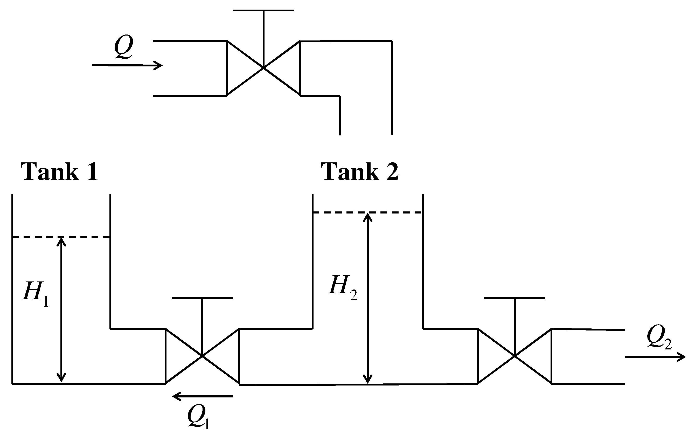
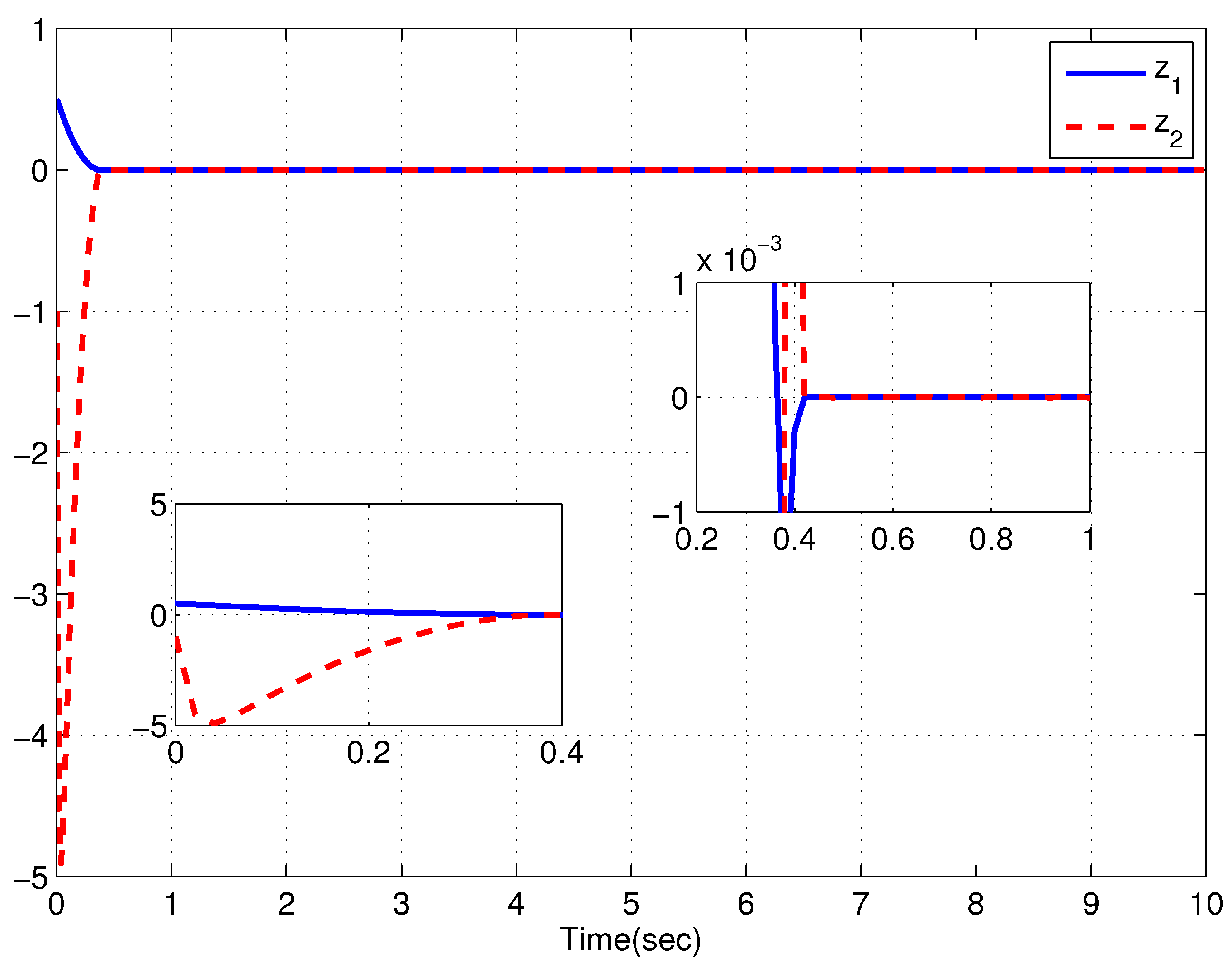
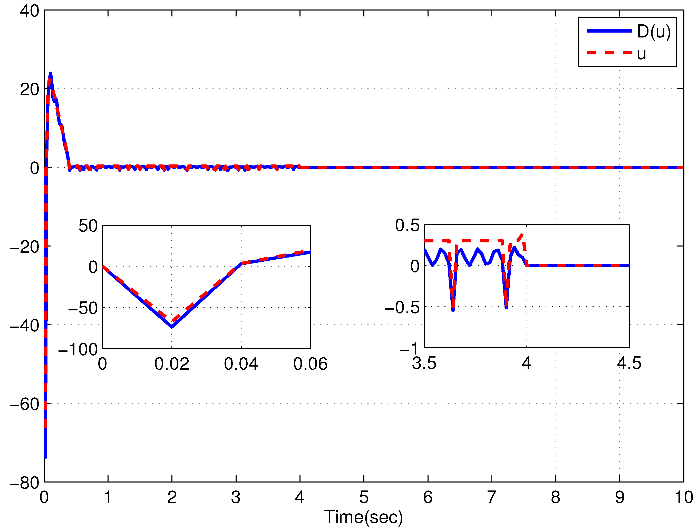
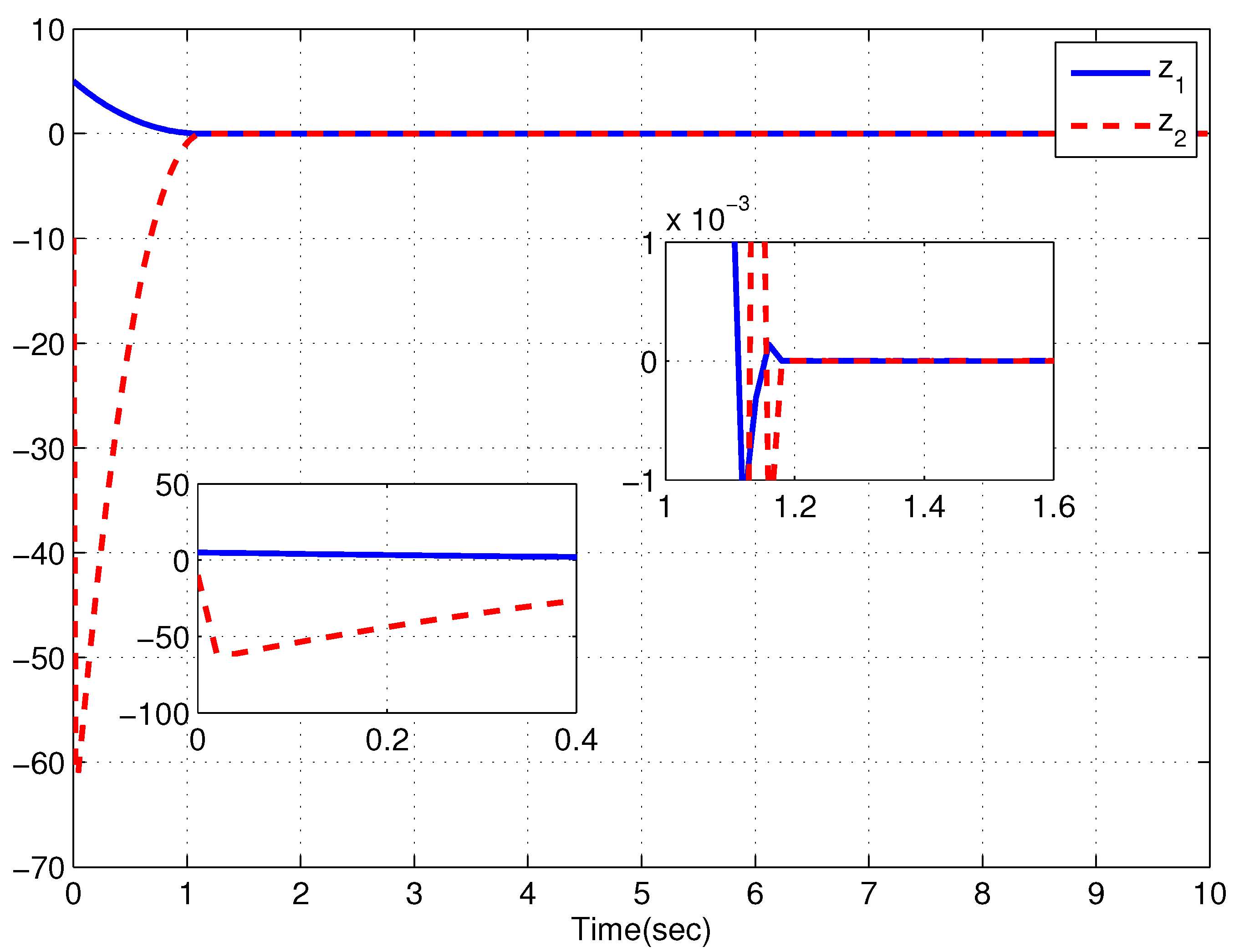
4. An Application Example

To verify the applicability of the proposed control scheme, we consider a liquid-level system exhibited in Figure 1, the dynamics of which are represented by

$$\begin{array}{ccc}{C}_1{\dot{H}}_1\hfill & =\hfill & Q_1\hfill \\ C_2{\dot{H}}_2\hfill & =\hfill & Q-Q_1-Q_2\hfill \\ Q_1\hfill & =\hfill & \left\{\begin{array}{c}{k}_1\sqrt{2g|H_2-H_1|},H_2\ge H_1,\hfill \\ -k_1\sqrt{2g|H_2-H_1|},H_2<H_1,\hfill \end{array}\right.\hfill \\ Q_2\hfill & =\hfill & k_2\sqrt{2g{H}_2},\hfill \end{array}$$

(45)

where the physical meanings of system parameters are as

$H_i$	liquid levels of tank i;
H	steady-state liquid levels of two tanks;
$C_i$	cross sections of tank i;
$k_1$	cross sections of the inlet manual valves of tanks 1 and 2;
$k_2$	cross sections of the right outlet manual valves of tank 2;
Q	inflow rate of this system;
$Q_1$	inflow rate from tank 2 to tank 1;
$Q_2$	outflow rate of this system;
g	gravitational acceleration.

By introducing the variable changes

$$\begin{array}{c}{\displaystyle z_1=H_1-H,z_2=H_2-H_1,u=\frac{Q}{C_2}-\frac{k_2\sqrt{2gH}}{C_2},}\hfill \end{array}$$

(46)

and taking the input dead-zone nonlinearity into account, the dynamics of (45) can be further modeled as

$$\begin{array}{c}{\dot{z}}_1=d_1{\lceil z_2\rceil }^{\frac{1}{2}},\hfill \\ {\dot{z}}_2=D\left(u\right)+f_2\left({\overline{z}}_2\right),\hfill \end{array}$$

(47)

where $d_1=\frac{k_1\sqrt{2g}}{C_1}$ and $f_2\left({\overline{z}}_2\right)=-\frac{C_1}{C_2}{d}_1{\lceil z_2\rceil }^{\frac{1}{2}}-\frac{k_2\sqrt{2g}}{C_2}{\lceil z_1+z_2+H\rceil }^{\frac{1}{2}}+\frac{k_2\sqrt{2g}}{C_2}{\lceil H\rceil }^{\frac{1}{2}}$, D denotes the output of dead-zone input nonlinearity described by (2) with $m_r=m_l=1+0.1sint$, $b_r=0.2+0.1sint$ and $b_l=0.4+0.1cost$, respectively. Based on Lemma 4, it is easily verified that Assumptions 1–3 hold with ${\lambda }_3=\tau =1$, ${\lambda }_1={\lambda }_2=2$, ${\underline{m}}_r={\underline{m}}_l=0.9$, ${\overline{b}}_r=0.3$, ${\overline{b}}_l=0.5$, ${\phi }_2=\frac{\sqrt{2g}}{C_2}(k_1+k_2)$.

Introducing ${\zeta }_i={ϝ}^{(1+c){\lambda }_i}{z}_i$, $i=1,2$ with

$$ϝ=\left\{\begin{array}{ccc}{\displaystyle \frac{T_s}{T_s-t},}\hfill & \hfill & \zeta \in \{{\mathbb{R}}^2-\mathsf{\Xi }\}\&t<T_s,\hfill \\ {\displaystyle 1,}\hfill & \hfill & \mathrm{otherwise},\hfill \end{array}\right.$$

(48)

where $\mathsf{\Xi }$ is a small closed neighborhood of origin and taking $\rho =2$ and $c=0$, according to Theorem 1, one can design a state feedback controller

$$u=\left\{\begin{array}{ccc}{\displaystyle \left(\frac{{ϝ}^{-1}{\zeta }_3^{*}}{{\underline{m}}_r}+{\overline{b}}_r\right),}\hfill & \hfill & {\zeta }_3^{*}>0,\hfill \\ 0,\hfill & \hfill & {\zeta }_3^{*}=0,\hfill \\ {\displaystyle \left(\frac{{ϝ}^{-1}{\zeta }_3^{*}}{{\underline{m}}_l}-{\overline{b}}_l\right),}\hfill & \hfill & {\zeta }_3^{*}<0,\hfill \end{array}\right.$$

(49)

$$\begin{array}{c}{\zeta }_3^{*}=-\left(0.1+{\varrho }_{21}+{\varrho }_{22}+{\varrho }_{23}\right){\lceil {\pi }_2\rceil }^{\frac{1}{2}},\hfill \end{array}$$

(50)

with ${\beta }_1=(1.1+\frac{2}{T_s}{(1+{\zeta }_1^2)}^{\frac{1}{2}})/d_1$ if $\zeta \in \{{\mathbb{R}}^2-\mathsf{\Xi }\}\&t<T_s$ and ${\beta }_1=1.1/d_1$ otherwise, ${\pi }_2={\zeta }_2-{\zeta }_2^{*}$, ${\zeta }_2^{*}=-{\beta }_1{\zeta }_1^2$, ${\tilde{\phi }}_2=(1+{\beta }_1^{\frac{1}{2}})(1+c){\lambda }_2{\left|{\zeta }_2\right|}^{\tau /{\lambda }_2}/T_s+{\phi }_2$, ${\varrho }_{21}=3.7712d_1^{\frac{3}{2}}$, ${\varrho }_{22}=0.6667{\tilde{\phi }}_2^{\frac{3}{2}}+{\tilde{\phi }}_2$, ${\varrho }_{23}=|\frac{\partial {\zeta }_2^{*}}{\partial {\zeta }_1}{d}_1|+0.6667|\frac{\partial {\zeta }_2^{*}}{\partial {\zeta }_1}{|}^3{(d_1{\beta }_1^{\frac{1}{2}}+\frac{2}{T_s}{(1+{\zeta }_1^2)}^{\frac{1}{2}})}^3$, which can render the system (47) globally prescribed-time stable.

For the simplicity, take the system parameters as $H=100 \mathrm{cm}$, $g=9.8 \mathrm{m}/{\mathrm{s}}^2$, $C_1=C_2=\sqrt{2g}=4.427 {\mathrm{cm}}^2$, $k_1=1 {\mathrm{cm}}^2$ and $k_2=0.25 {\mathrm{cm}}^2$ and the prescribed time as $T_p=4s$, $T_s=3.8 s$, $\mathsf{\Xi }=\{\zeta :{\zeta }_1^2+{\zeta }_2^2\le 0.01\}$. For $(z_1\left(0\right),z_2\left(0\right))=(0.5,-1)$ and $(z_1\left(0\right),z_2\left(0\right))=(5,-10)$, Figure 2, Figure 3, Figure 4 and Figure 5 are given to exhibit the responses of the CLS via MATLAB2020. It can be clearly observed that the convergence time of the system maintains below the prescribed time 4 s, which confirms the effectiveness of the control scheme.

To text the robustness of the proposed controller, the external disturbance $\omega \left(t\right)=0.1sint$ is introduced in the input channel. With the same parameters, the responses of the CLS are given in Figure 6 and Figure 7, from which it is observed that the proposed controller is robust against small external disturbances.

5. Conclusions

In this paper, a global prescribed-time stabilizing controller has been developed for a kind of HONSs with asymmetric actuator dead-zone. Due to the novel introduced SST, the significant advantage of the presented scheme is that its settling time can be preset and adjusted arbitrarily according to practical requirements by choosing the positive design parameter $T_s$. How to develop a prescribed-time controller for HONSs with parameter uncertainty and/or disturbances will be a topic for our future works. Applying the proposed method to practical systems such as rigid bodies [45], quadrotor UAVs [46] and induction motors [47] is another of our future topics.

References

1. Rui, C.; Reyhanoglu, M.; Kolmanovsky, I.; Cho, S.; McClamroch, N.H. Nonsmooth stabilization of an underactuated unstable two degrees of freedom mechanical system. Proc. IEEE Conf. Decis. Control 1997, 4, 3998–4003. [Google Scholar]
2. Cheng, D.; Lin, W. On p-normal forms of nonlinear systems. IEEE Trans. Autom. Control 2003, 48, 1242–1248. [Google Scholar] [CrossRef] [Green Version]
3. Lin, W.; Qian, C. Adding one power integrator: A tool for global stabilization of high order lower-triangular systems. Syst. Control Lett. 2000, 39, 339–351. [Google Scholar] [CrossRef]
4. Ding, S.; Li, S.; Zheng, W.X. Nonsmooth stabilization of a class of nonlinear cascaded systems. Automatica 2012, 48, 2597–2606. [Google Scholar] [CrossRef]
5. Gao, F.; Wu, Y. Global state feedback stabilisation for a class of more general high-order non-linear systems. IET Control Theory Appl. 2014, 8, 1648–1655. [Google Scholar] [CrossRef]
6. Sun, Z.Y.; Zhang, C.H.; Wang, Z. Adaptive disturbance attenuation for generalized high-order uncertain nonlinear systems. Automatica 2017, 80, 102–109. [Google Scholar] [CrossRef]
7. Chen, C.C.; Chen, G.S. A new approach to stabilization of high-order nonlinear systems with an asymmetric output constraint. Int. J. Robust Nonlinear Control 2020, 30, 756–775. [Google Scholar] [CrossRef]
8. Bhat, S.P.; Bernstein, D.S. Finite-time stability of continuous autonomous systems. SIAM J. Control Optim. 2000, 38, 751–766. [Google Scholar] [CrossRef]
9. Huang, X.; Lin, W.; Yang, B. Global finite-time stabilization of a class of uncertain nonlinear systems. Automatica 2005, 41, 881–888. [Google Scholar] [CrossRef]
10. Liu, Y. Global finite-time stabilization via time-varying feedback for uncertain nonlinear systems. SIAM J. Control Optim. 2014, 52, 1886–1913. [Google Scholar] [CrossRef]
11. Sun, Z.Y.; Xue, L.R.; Zhang, K. A new approach to finite-time adaptive stabilization of high-order uncertain nonlinear system. Automatica 2015, 58, 60–66. [Google Scholar] [CrossRef]
12. Fu, J.; Ma, R.; Chai, T. Global finite-time stabilization of a class of switched nonlinear systems with the powers of positive odd rational numbers. Automatica 2015, 54, 360–373. [Google Scholar] [CrossRef]
13. Fu, J.; Ma, R.; Chai, T. Adaptive finite-time stabilization of a class of uncertain nonlinear systems via logic-based switchings. IEEE Trans. Autom. Control 2017, 62, 5998–6003. [Google Scholar] [CrossRef]
14. Sun, Z.Y.; Shao, Y.; Chen, C.C. Fast finite-time stability and its application in adaptive control of high-order nonlinear system. Automatica 2019, 106, 339–348. [Google Scholar] [CrossRef]
15. Picó, J.; Picó-Marco, E.; Vignoni, A.; De Battista, H. Stability preserving maps for finite-time convergence: Super-twisting sliding-mode algorithm. Automatica 2013, 49, 534–539. [Google Scholar] [CrossRef]
16. Chen, C.C.; Sun, Z.Y. A unified approach to finite-time stabilization of high-order nonlinear systems with an asymmetric output constraint. Automatica 2020, 111, 108581. [Google Scholar] [CrossRef]
17. Chen, C.C.; Sun, Z.Y. Output feedback finite-time stabilization for high-order planar systems with an output constraint. Automatica 2020, 114, 108843. [Google Scholar] [CrossRef]
18. Andrieu, V.; Praly, L.; Astolfi, A. Homogeneous approximation, recursive observer design, and output feedback. SIAM J. Control Optim. 2008, 47, 1814–1850. [Google Scholar] [CrossRef] [Green Version]
19. Tian, B.; Zuo, Z.; Yan, X.; Wang, H. A fixed-time output feedback control scheme for double integrator systems. Automatica 2017, 80, 17–24. [Google Scholar] [CrossRef] [Green Version]
20. Polyakov, A. Nonlinear feedback design for fixed-time stabilization of linear control systems. IEEE Trans. Autom. Control 2012, 57, 2106–2110. [Google Scholar] [CrossRef] [Green Version]
21. Zuo, Z. Nonsingular fixed-time consensus tracking for second-order multi-agent networks. Automatica 2015, 54, 305–309. [Google Scholar] [CrossRef]
22. Defoort, M.; Demesure, G.; Zuo, Z.; Polyakov, A.; Djemai, M. Fixed-time stabilisation and consensus of non-holonomic systems. IET Control Theory Appl. 2016, 10, 2497–2505. [Google Scholar] [CrossRef]
23. Basin, M.; Rodríguez-Ramírez, P.; Avellaneda, F.G. Continuous fixed-time controller design for mechatronic systems with incomplete measurements. IEEE/ASME Trans. Mechatronics 2016, 23, 57–67. [Google Scholar] [CrossRef]
24. Chen, C.C.; Sun, Z.Y. Fixed-time stabilisation for a class of high-order non-linear systems. IET Control Theory Appl. 2018, 12, 2578–2587. [Google Scholar] [CrossRef]
25. Gao, F.; Wu, Y.; Zhang, Z.; Liu, Y. Global fixed-time stabilization for a class of switched nonlinear systems with general powers and its application. Nonlinear Anal. Hybrid Syst. 2019, 31, 56–68. [Google Scholar] [CrossRef]
26. Wang, G.; Wang, B.; Zhang, C. Fixed-time third-order super-twisting-like sliding mode motion control for piezoelectric nanopositioning stage. Mathematics 2021, 9, 1770. [Google Scholar] [CrossRef]
27. Ning, B.; Han, Q.L. Prescribed finite-time consensus tracking for multi-agent systems with nonholonomic chained-form dynamics. IEEE Trans. Autom. Control 2019, 64, 1686–1693. [Google Scholar] [CrossRef]
28. Zuo, Z.; Defoort, M.; Tian, B.; Ding, Z. Distributed consensus observer for multi-agent systems with high-order integrator dynamics. IEEE Trans. Autom. Control 2019, 65, 1771–1778. [Google Scholar] [CrossRef] [Green Version]
29. Zarchan, P. Tactical and Strategic Missile Guidance; American Institute of Aeronautics and Astronautics (AIAA): Reston, VA, USA, 2007. [Google Scholar]
30. Song, Y.; Wang, Y.; Holloway, J.; Krstic, M. Time-varying feedback for regulation of normal-form nonlinear systems in prescribed finite time. Automatica 2017, 83, 243–251. [Google Scholar] [CrossRef]
31. Sánchez-Torres, J.D.; Defoort, M.; Munoz-Vázquez, A.J. Predefined-time stabilisation of a class of nonholonomic systems. Int. J. Control 2020, 93, 2941–2948. [Google Scholar] [CrossRef]
32. Cao, Y.; Wen, C.; Tan, S.; Song, Y. Prespecifiable fixed-time control for a class of uncertain nonlinear systems in strict-feedback form. Int. J. Robust Nonlinear Control 2020, 30, 1203–1222. [Google Scholar] [CrossRef]
33. Gao, F.; Wu, Y.; Zhang, Z. Global fixed-time stabilization of switched nonlinear systems: A time-varying scaling transformation approach. IEEE Trans. Circuits Syst. II Exp. Briefs 2019, 66, 1890–1894. [Google Scholar] [CrossRef]
34. Seeber, R.; Haimovich, H.; Horn, M.; Fridman, L.M.; De Battista, H. Robust exact differentiators with predefined convergence time. Automatica 2021, 134, 109858. [Google Scholar] [CrossRef]
35. Kairuz, R.I.V.; Orlov, Y.; Aguilar, L.T. Prescribed-time stabilization of controllable planar systems using switched state feedback. IEEE Control Syst. Lett. 2021, 5, 2048–2053. [Google Scholar] [CrossRef]
36. Tao, G.; Kokotovic, P.V. Adaptive control of plants with unknown dead-zones. IEEE Trans. Autom. Control 1994, 39, 59–68. [Google Scholar]
37. Zhao, X.; Shi, P.; Zheng, X.; Zhang, L. Adaptive tracking control for switched stochastic nonlinear systems with unknown actuator dead-zone. Automatica 2015, 60, 193–200. [Google Scholar] [CrossRef]
38. Zhang, Z.; Xu, S.; Zhang, B. Exact tracking control of nonlinear systems with time delays and dead-zone input. Automatica 2015, 52, 272–276. [Google Scholar] [CrossRef]
39. Zhang, Z.; Park, J.H.; Zhang, K.; Lu, J. Adaptive control for a class of nonlinear time-delay systems with dead-zone input. J. Frankl. Inst. 2016, 353, 4400–4421. [Google Scholar] [CrossRef]
40. Hua, C.; Li, Y.; Guan, X. Finite/fixed-time stabilization for nonlinear interconnected systems with dead-zone input. IEEE Trans. Autom. Control 2017, 62, 2554–2560. [Google Scholar] [CrossRef]
41. Gao, F.; Wu, Y.; Liu, Y. Finite-time stabilization for a class of switched stochastic nonlinear systems with dead-zone input nonlinearities. Int. J. Robust Nonlinear Control 2018, 28, 3239–3257. [Google Scholar] [CrossRef]
42. Gao, F.; Shang, Y.; Wu, Y.; Liu, Y. Global fixed-time stabilization for a class of uncertain high-order nonlinear systems with dead-zone input nonlinearity. Trans. Inst. Meas. Control 2019, 41, 1888–1895. [Google Scholar] [CrossRef]
43. Ding, S.; Chen, W.H.; Mei, K.; Murray-Smith, D. Disturbance observer design for nonlinear systems represented by input-output models. IEEE Trans. Ind. Electron. 2019, 67, 1222–1232. [Google Scholar] [CrossRef] [Green Version]
44. Khalil, H.K. Nonlinear Systems, 3rd ed.; Prentice-Hall: Hoboken, NJ, USA, 2002. [Google Scholar]
45. Golestani, M.; Mobayen, S.; Din, S.U.; El-Sousy, F.F.; Vu, M.T.; Assawinchaichote, W. Prescribed performance attitude stabilization of a rigid body under physical limitations. IEEE Trans. Aerosp. Electron. Syst. 2022. [Google Scholar] [CrossRef]
46. Mobayen, S.; Pouzesh, M. Event-triggered fractional-order sliding mode control technique for stabilization of disturbed quadrotor unmanned aerial vehicles. Aerosp. Sci. Technol. 2022, 121, 107337. [Google Scholar]
47. Sabzalian, M.H.; Alattas, K.A.; El-Sousy, F.F.M.; Mohammadzadeh, A.; Mobayen, S.; Vu, M.T.; Aredes, M. A neural controller for induction motors: Fractional-order stability analysis and online learning algorithm. Mathematics 2022, 10, 1003. [Google Scholar] [CrossRef]
Figure 1. Schematic diagram of the liquid-level system.
Mathematics 10 02147 g001
Figure 2. The state responses of the CLS with initial condition ( z 1 ( 0 ) , z 2 ( 0 ) ) = ( 0.5 , 1 ) .
Mathematics 10 02147 g002
Figure 3. The input responses of the CLS with initial condition ( z 1 ( 0 ) , z 2 ( 0 ) ) = ( 0.5 , 1 ) .
Mathematics 10 02147 g003
Figure 4. The state responses of the CLS with initial condition ( z 1 ( 0 ) , z 2 ( 0 ) ) = ( 5 , 10 ) .
Mathematics 10 02147 g004
Figure 5. The input responses of the CLS with initial condition ( z 1 ( 0 ) , z 2 ( 0 ) ) = ( 5 , 10 ) .
Mathematics 10 02147 g005
Figure 6. The state responses of the CLS with external disturbance and initial condition ( z 1 ( 0 ) , z 2 ( 0 ) ) = ( 1 , 5 ) .
Mathematics 10 02147 g006
Figure 7. The input responses of the CLS with external disturbance and initial condition ( z 1 ( 0 ) , z 2 ( 0 ) ) = ( 1 , 5 ) .
Mathematics 10 02147 g007
Publisher’s Note: MDPI stays neutral with regard to jurisdictional claims in published maps and institutional affiliations.