
Study on a Quantitative Indicator for Surface Stability Evaluation of Limestone Strata with a Shallowly Buried Spherical Karst Cave


Abstract
:1. Introduction
2. Theoretical Analysis of Spatial Stress Distribution
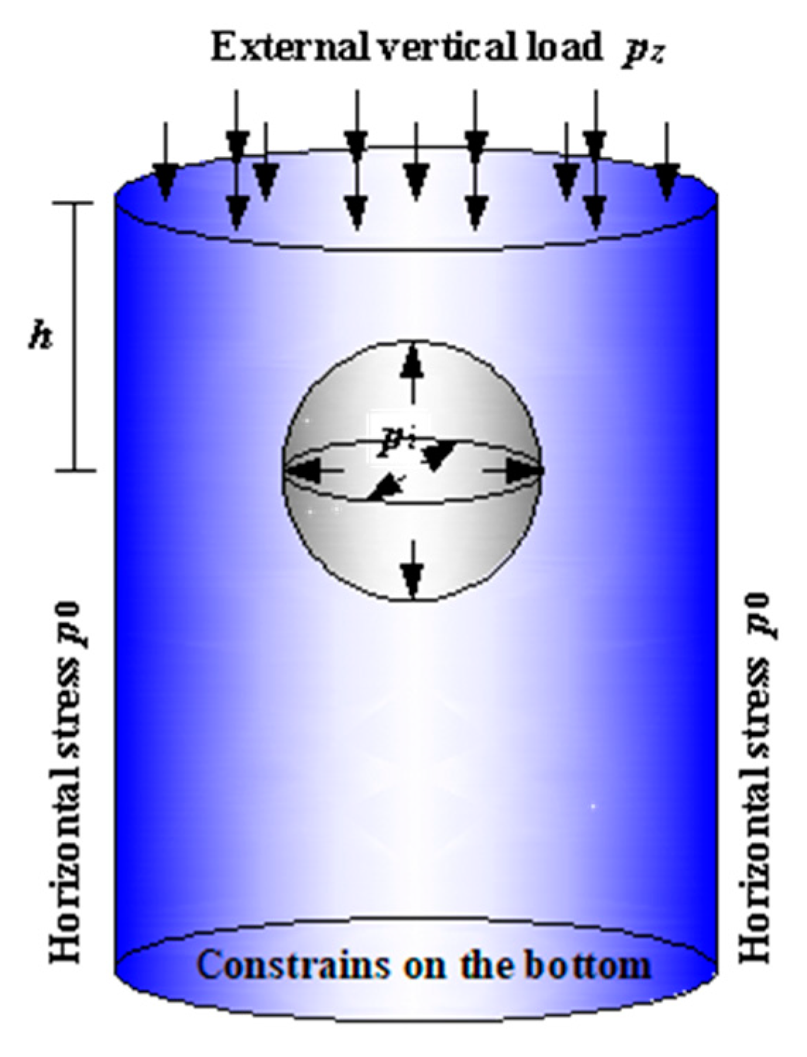
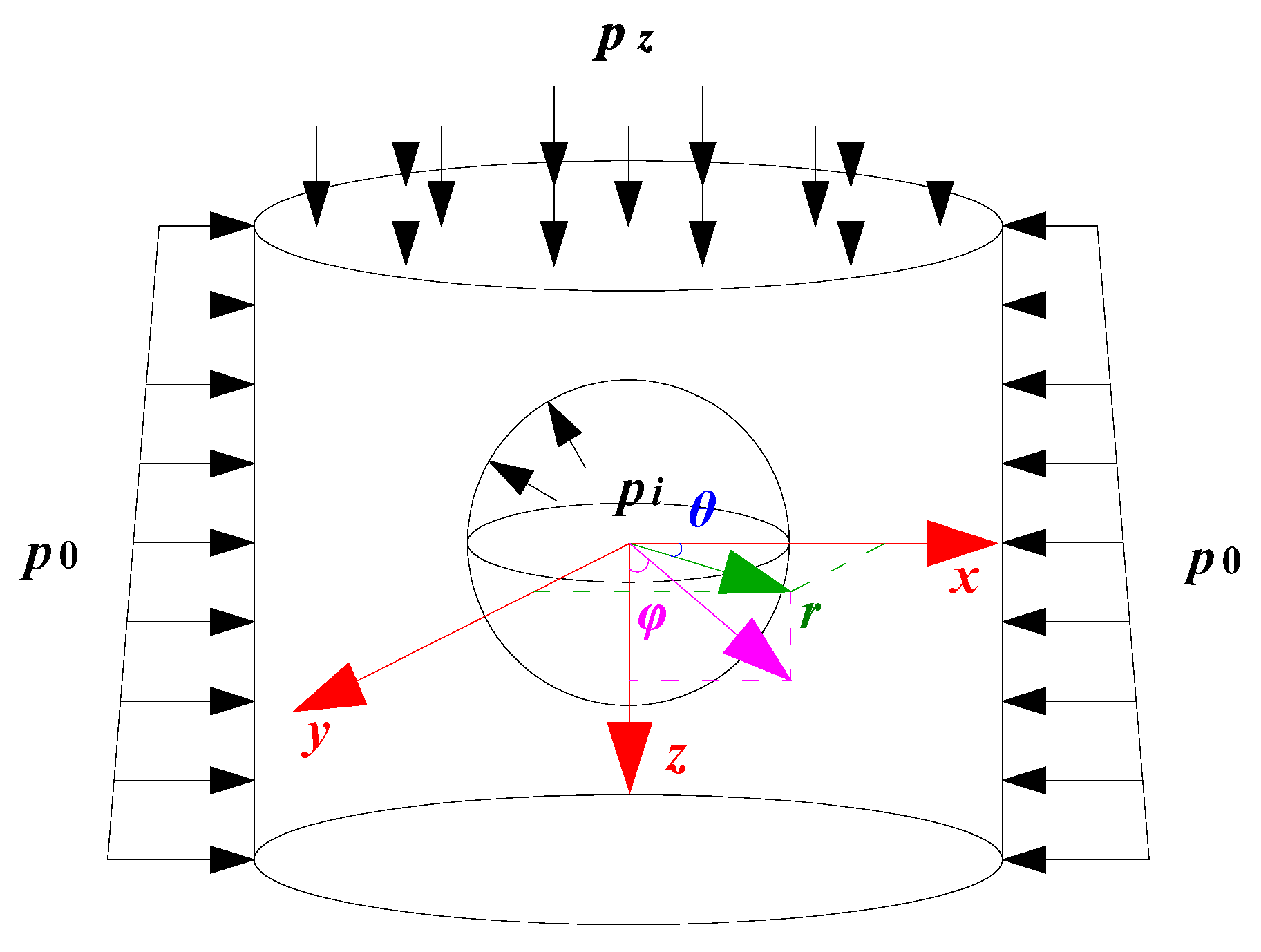
2.1. Mathematical Model and Boundary Conditions
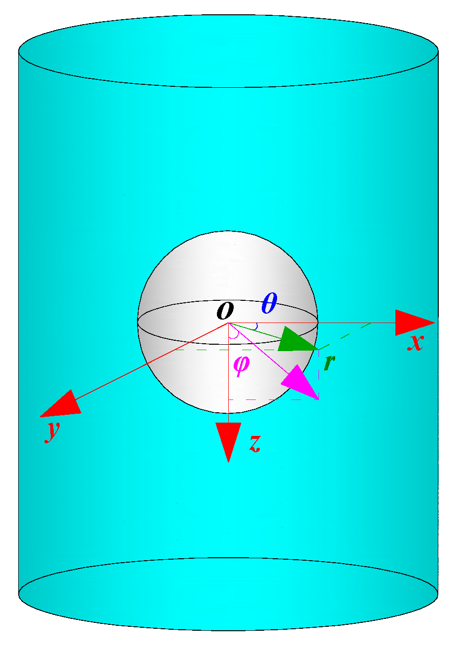
2.1.1. Mathematical Model
2.1.2. Boundary Conditions
- (1)
- , ;
- (2)
- , ;
- (3)
- , ;
- (4)
- , .
2.2. Theoretical Analysis
2.2.1. The Basic Theory
2.2.2. The General Solution
3. Bearing Capacity of Limestone Strata Roof
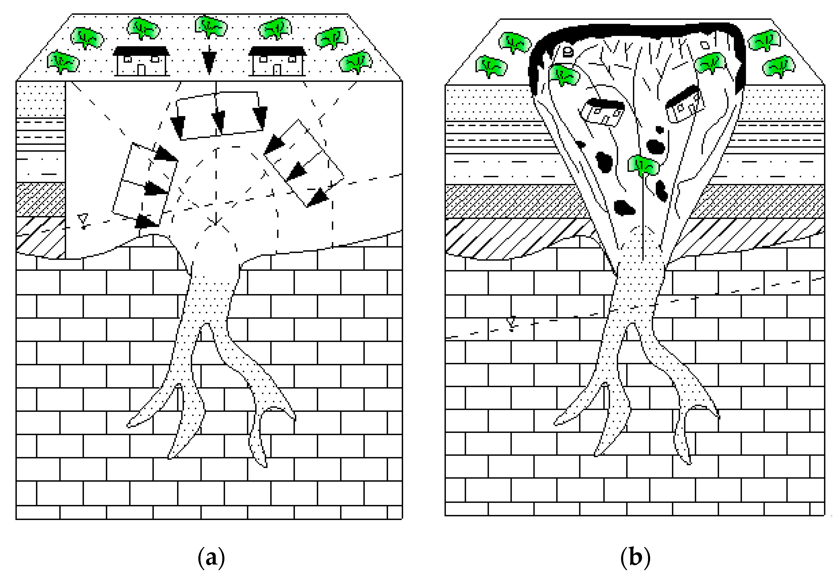
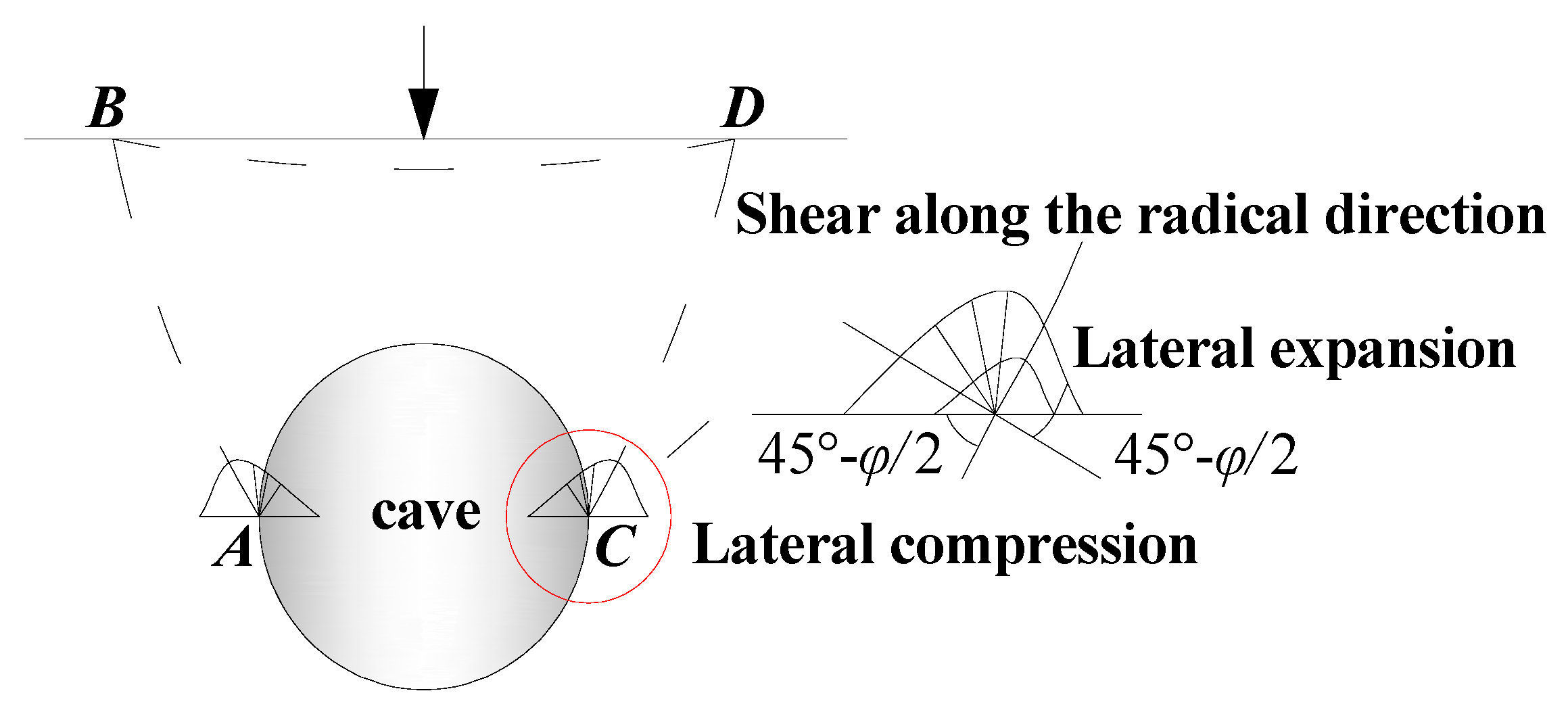
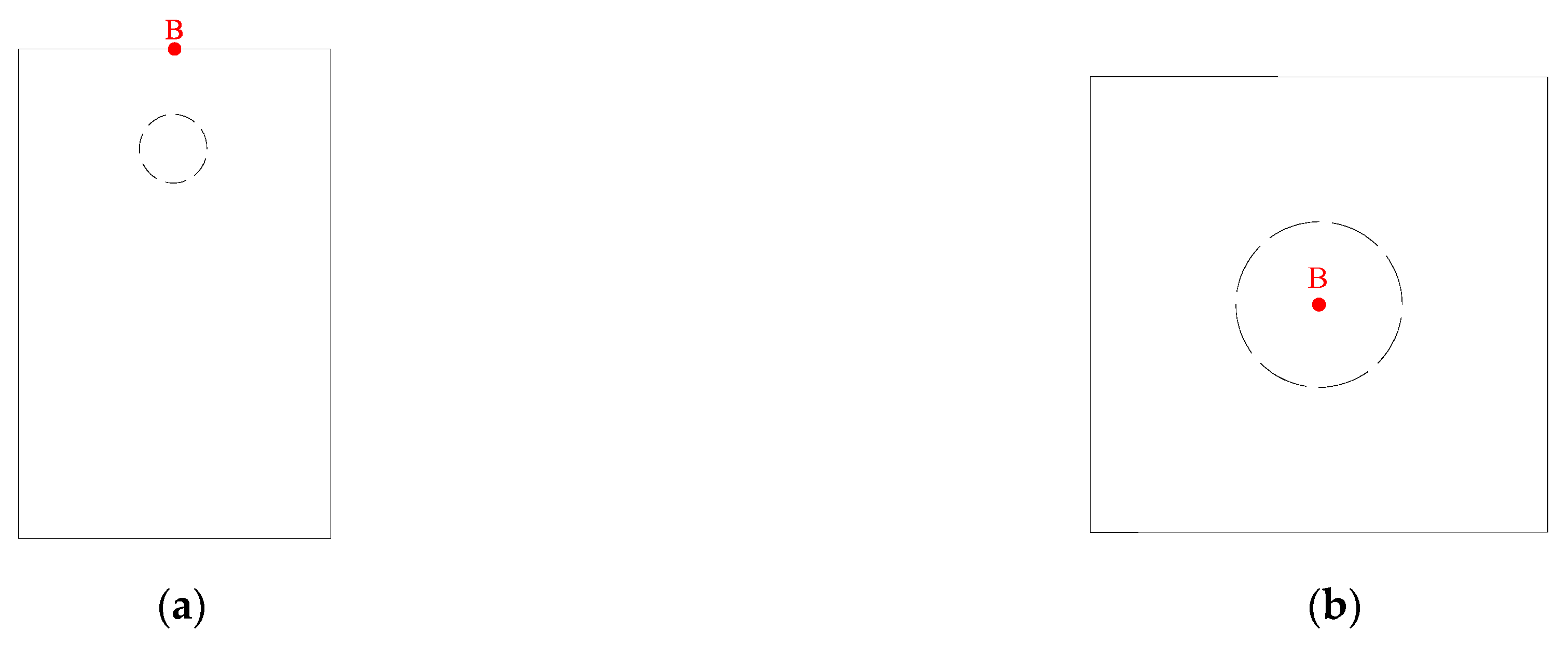
3.1. Failure Mechanism of Ground Collapse
3.2. Theoretical Analysis of Bearing Capacity
3.2.1. The Basic Theory
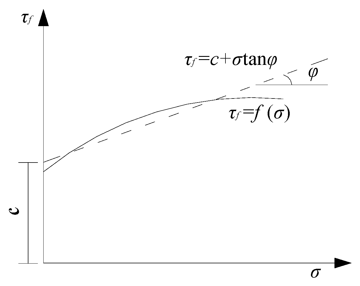
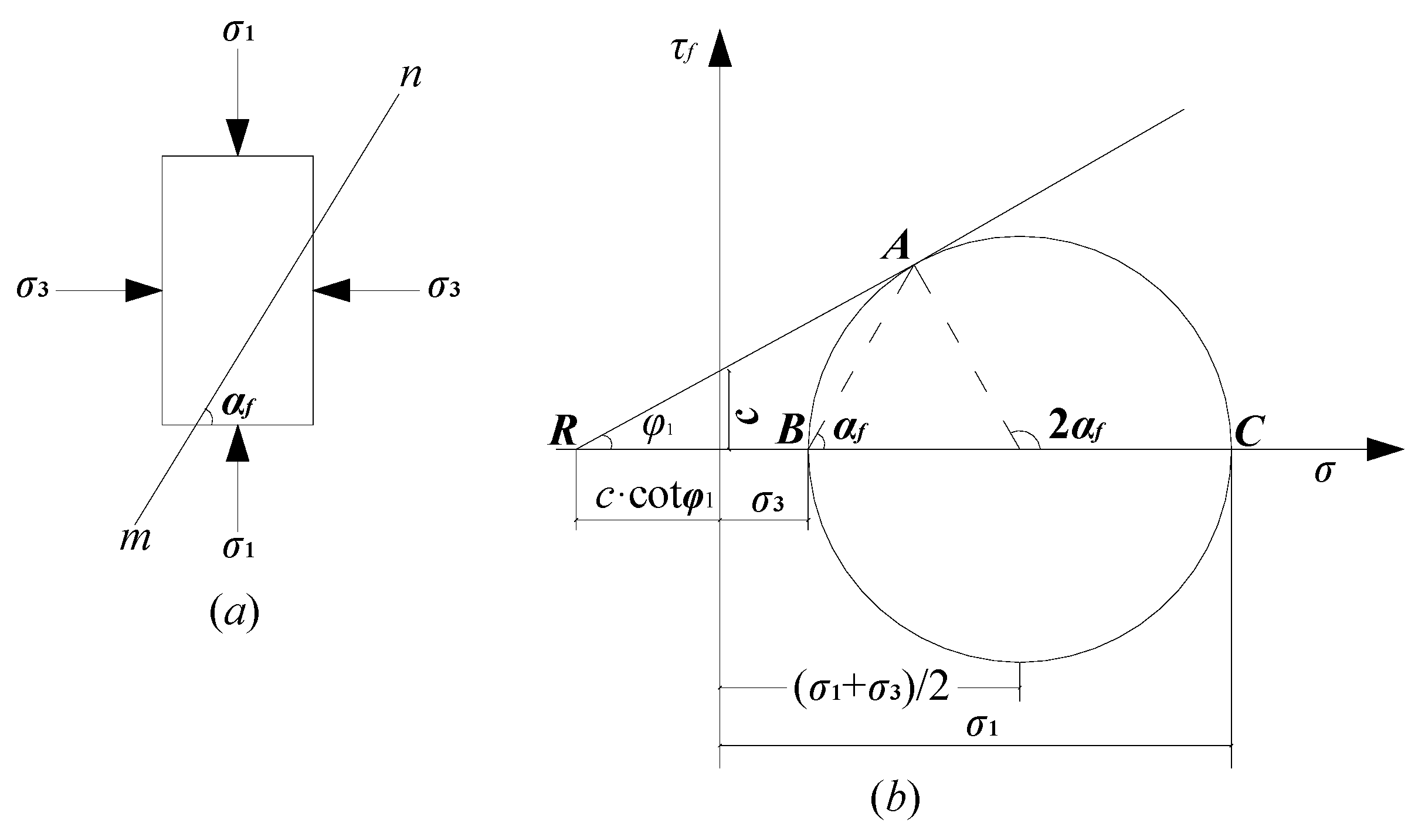
Mohr-Coulomb Strength Theory
Principle Stress of Any Point
Transformation of Stress Components in Different Coordinate Systems
3.3. General Solution of Bearing Capacity Calculation Formula
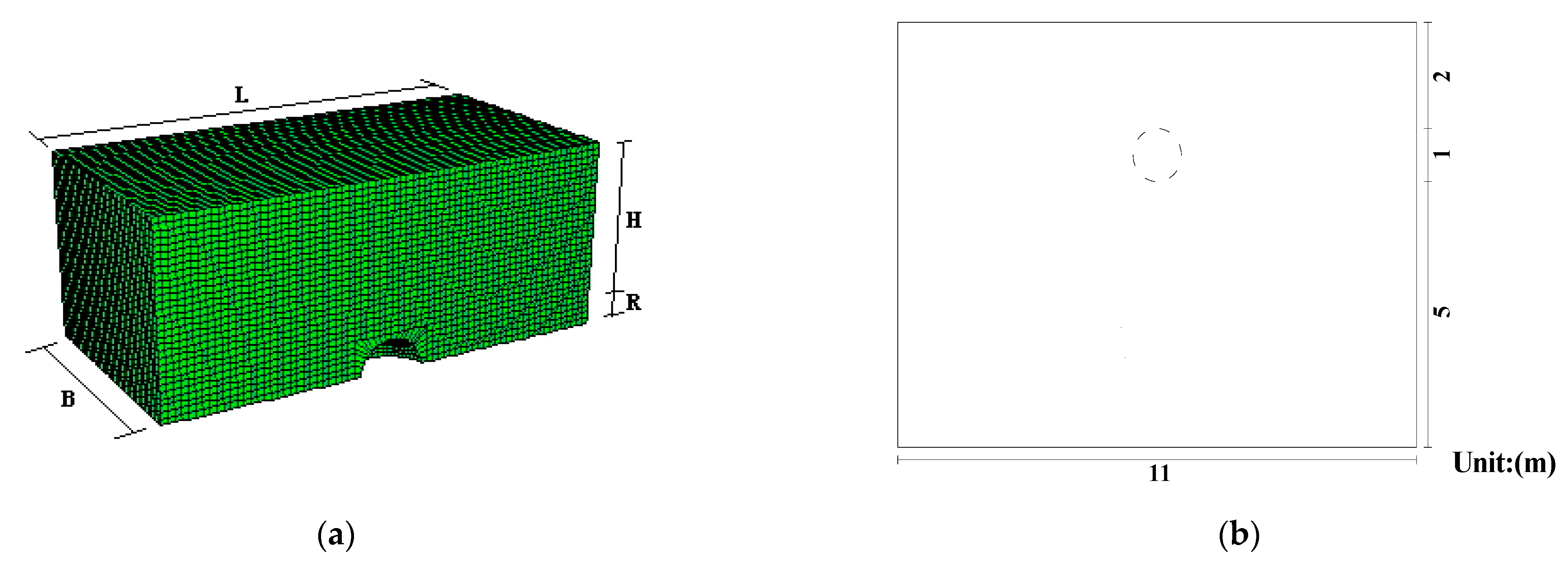
4. Application and Validation Test
5. Discussion
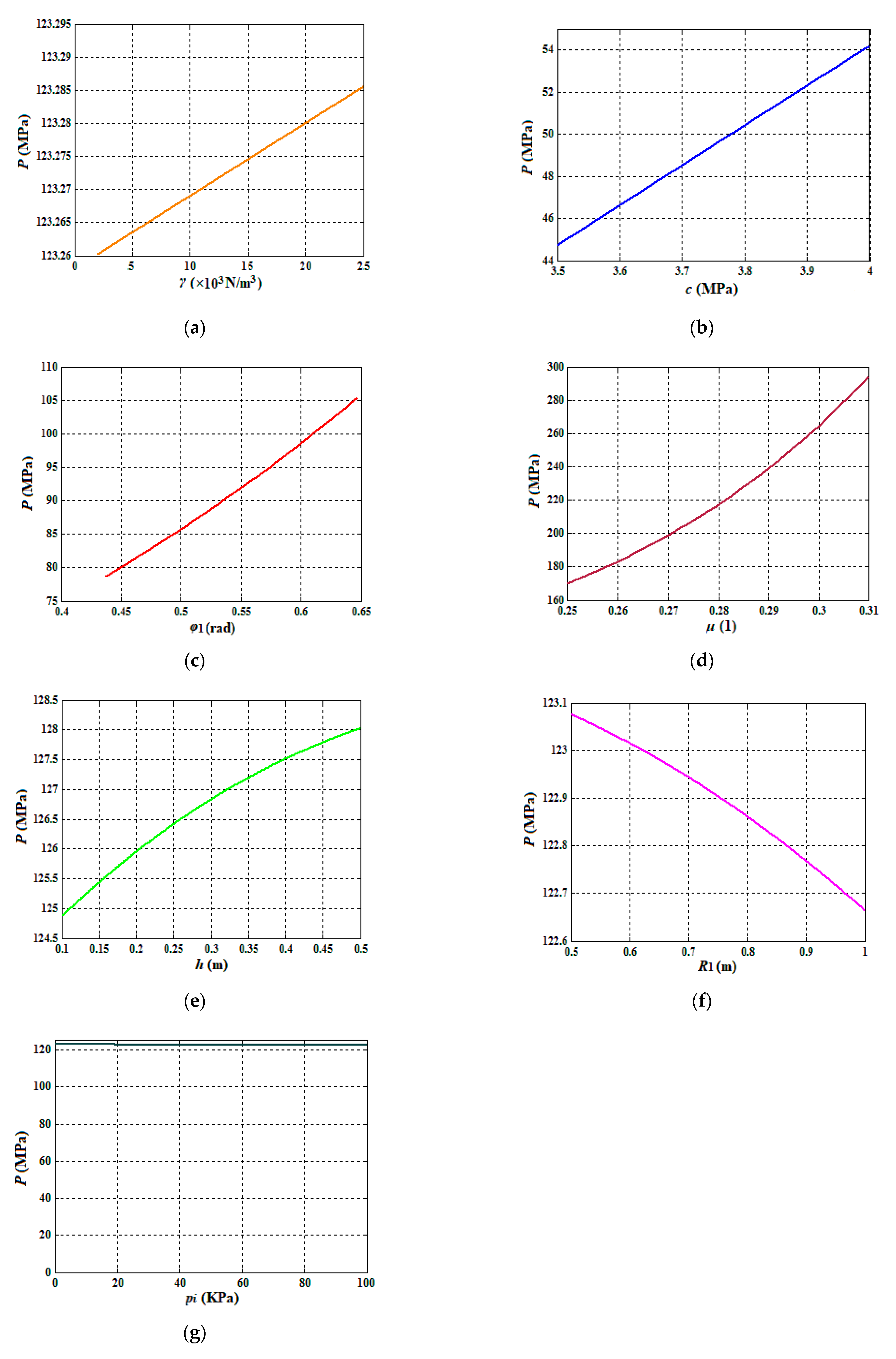
5.1. Bearing Capacity Change Caused by Various Factors
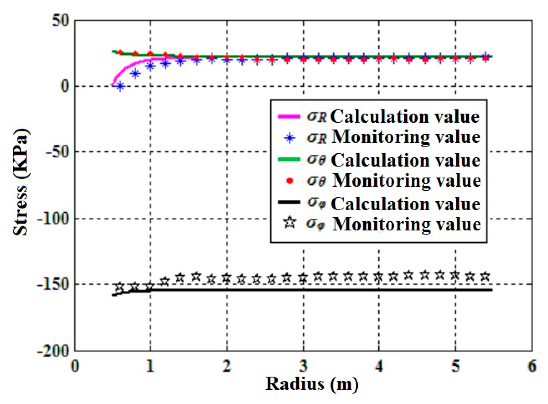
5.2. General Solution of Stress Components
6. Conclusions
Author Contributions
Funding
Institutional Review Board Statement
Informed Consent Statement
Conflicts of Interest
References
- Xie, P.; Wen, H.J.; Zhang, Y.Y.; Zhang, X.X.; Hu, J. A method for identification and reconstruction of hard structural planes, weak interlayer, and cavities in the limestone near surface. Eur. J. Environ. Civ. Eng. 2020, 24, 2489–2511. [Google Scholar] [CrossRef]
- Gutierrez, F.; Parise, M.; Dewaele, J.; Jourde, H. A review on natural and human-induced geohazards and impacts in karst. Earth-Sci. Rev. 2014, 138, 61–88. [Google Scholar] [CrossRef]
- Xie, P.; Wen, H.; Xiao, P.; Zhang, Y. Evaluation of ground-penetrating radar (GPR) and geology survey for slope stability study in mantled karst region. Environ. Earth Sci. 2018, 77, 122. [Google Scholar] [CrossRef]
- Xiao, X.X.; Gutiérrez, F.; Guerrero, J. The impact of groundwater drawdown and vacuum pressure on sinkhole development. Physical laboratory models. Eng. Geol. 2020, 279, 105894. [Google Scholar] [CrossRef]
- Wang, X.L.; Lai, J.X.; He, S.Y.; Garnes, R.S.; Zhang, Y.W. Karst geology and mitigation measures for hazards during metro system construction in Wuhan, China. Nat. Hazards 2020, 103, 2905–2927. [Google Scholar] [CrossRef]
- Yin, J.F.; Lei, Y.; Chen, Q.N. Summary about researches on the calculation method for the bearing capacity of cave roof. J. Hunan Univ. Arts Sci. 2017, 29, 68–72. (In Chinese) [Google Scholar]
- Goodier, J.N. Concentrations of stress around spheroidal and cylindrical inclusions and flaws. Trans. ASME J. Appl. Mech. 1933, 55, 39–44. [Google Scholar] [CrossRef]
- Howland, R.C.J.; Knight, R.C. Stress functions for a plate containing groups of circular holes. Philos. Trans. R. Soc. A 1939, 238, 357–392. [Google Scholar]
- Xu, X.; Fallahi, N.; Yang, H. Efficient CUF-based FEM analysis of thin-wall structures with Lagrange polynomial expansion. Mech. Adv. Mater. Struct. 2020, 29, 1316–1337. [Google Scholar] [CrossRef]
- Xu, X.; Yang, H. Vision Measurement of Tunnel Structures with Robust Modelling and Deep Learning Algorithms. Sensors 2020, 20, 4945. [Google Scholar] [CrossRef] [PubMed]
- Xu, X.; Shi, P.; Zhou, X.; Liu, W.; Yang, H.; Wang, T.; Yan, M.; Fan, W. A novel vision measurement system for health monitoring of tunnel structures. Mech. Adv. Mater. Struct. 2020, 29, 2208–2218. [Google Scholar] [CrossRef]
- Xie, P.; Ma, S.K.; Wen, H.J.; Li, L.Y.; Jie, S.L.; Li, R.B. Theoretical analysis on stress distribution characteristics around a shallow buried cylinder Karst cave containing filling in limestone strata. Arab. J. Geosci. 2022, 15, 224. [Google Scholar] [CrossRef]
- Xie, P.; Ma, S.K.; Wen, H.J.; Li, L.Y. Theoretical analysis on stress distribution characteristics around a shallow buried spherical Karst cave containing fill materials in limestone strata. Environ. Earth Sci. 2022, 81, 97. [Google Scholar] [CrossRef]
- Zhao, H.; Xiao, Y.; Zhao, M.H.; Yang, C.W. Stability assessment method for subgrade with underlying rectangular cavity. China J. Highw. Transp. 2018, 31, 165–180. [Google Scholar]
- Xie, P.; Wen, H.J.; Ma, S.K.; Yue, Z.R.; Li, L.Y.; Liu, J.F.; Li, R.B.; Cui, J. The bearing capacity analysis of limestone strata roof containing a shallow buried cylinder Karst cave. Mech. Adv. Mater. Struct. 2021, 1–8. [Google Scholar] [CrossRef]
- Lei, Y.; Deng, J.Z.; Liu, Z.Y.; Li, J.J.; Zou, G. A method to calculate ultimate bearing capacity of rock foundation with cavities considering load position offset. Rock Soil Mech. 2020, 41, 3326–3332. (In Chinese) [Google Scholar]
- Keawsawasvong, S.; Ukritchon, B. Undrained stability of a spherical cavity in cohesive soils using finite element limit analysis. J. Rock Mech. Geotech. Eng. 2019, 11, 1274–1285. [Google Scholar] [CrossRef]
- Keawsawasvong, S.; Ukritchon, B. Design equation for stability of shallow unlined circular tunnels in Hoek-Brown rock masses. Bull. Eng. Geol. Environ. 2020, 79, 4167–4190. [Google Scholar] [CrossRef]
- Keawsawasvong, S. Limit analysis solutions for spherical cavities in sandy soils under overloading. Innov. Infrastruct. Solut. 2021, 6, 33. [Google Scholar] [CrossRef]
- Keawsawasvong, S.; Shiau, J. Stability of Spherical Cavity in Hoek–Brown Rock Mass. Rock Mech. Rock Eng. 2022, 1–12. [Google Scholar] [CrossRef]
- Timoshenko, S.; Goodier, J.N. Theory of Elasticity; Xu, Z.; Wu, Y., Translators; Higher Education Press: Beijing, China, 1965. [Google Scholar]


| Parameters | γ (kN/m3) | E (GPa) | c (MPa) | φ (°) | μ | R1 (m) | pz (KPa) | pi (KPa) | h (m) | |
|---|---|---|---|---|---|---|---|---|---|---|
| Materials | ||||||||||
| Limestone strata | 26,500 | 35 | 7.8 | 42.3 | 0.25 | 0.5 | 0 | 0 | 2 | |
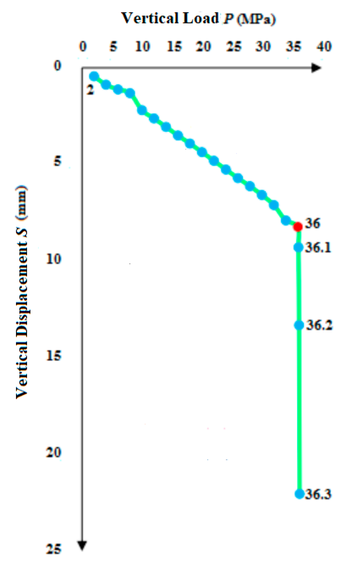
| Serial Number | External Vertical P (MPa) | Subsidence S (mm) |
|---|---|---|
| 1 | 2 | 0.437865 |
| 2 | 4 | 0.874118 |
| 3 | 6 | 1.12011 |
| 4 | 8 | 1.3118 |
| 5 | 10 | 2.19316 |
| 6 | 12 | 2.61823 |
| 7 | 14 | 3.05638 |
| 8 | 16 | 3.5 |
| 9 | 18 | 3.91891 |
| 10 | 20 | 4.36046 |
| 11 | 22 | 4.80857 |
| 12 | 24 | 5.2625 |
| 13 | 26 | 5.7035 |
| 14 | 28 | 6.1208 |
| 15 | 30 | 6.5762 |
| 16 | 32 | 7.10112 |
| 17 | 34 | 7.89486 |
| 18 | 36 | 8.22704 |
| 19 | 36.1 | 9.28338 |
| 20 | 36.2 | 13.3104 |
| 21 | 36.3 | 22.0348 |
Publisher’s Note: MDPI stays neutral with regard to jurisdictional claims in published maps and institutional affiliations. |
© 2022 by the authors. Licensee MDPI, Basel, Switzerland. This article is an open access article distributed under the terms and conditions of the Creative Commons Attribution (CC BY) license (https://creativecommons.org/licenses/by/4.0/).
Share and Cite
Xie, P.; Duan, H.; Wen, H.; Yang, C.; Ma, S.; Yue, Z. Study on a Quantitative Indicator for Surface Stability Evaluation of Limestone Strata with a Shallowly Buried Spherical Karst Cave. Mathematics 2022, 10, 2149. https://doi.org/10.3390/math10122149
Xie P, Duan H, Wen H, Yang C, Ma S, Yue Z. Study on a Quantitative Indicator for Surface Stability Evaluation of Limestone Strata with a Shallowly Buried Spherical Karst Cave. Mathematics. 2022; 10(12):2149. https://doi.org/10.3390/math10122149
Chicago/Turabian StyleXie, Peng, Huchen Duan, Haijia Wen, Chao Yang, Shaokun Ma, and Zurun Yue. 2022. "Study on a Quantitative Indicator for Surface Stability Evaluation of Limestone Strata with a Shallowly Buried Spherical Karst Cave" Mathematics 10, no. 12: 2149. https://doi.org/10.3390/math10122149