WAVECNV: A New Approach for Detecting Copy Number Variation by Wavelet Clustering

Abstract

Copy number variation (CNV) detection based on second-generation sequencing technology is the basis of much gene research, but the read depth is affected by mapping errors, repeated reads, and GC bias. The existing methods have low sensitivity to variation regions with a short length and small variation range. Therefore, it is necessary to improve the sensitivity of algorithms to short-variation fragments. This study proposes a new CNV-detection method named WAVECNV to solve this issue. The algorithm uses wavelet clustering to process the read depth and determine the normal cluster and abnormal cluster according to the size of the cluster. Then, according to the distance between genome bins and normal clusters, the outlier of each genome bin is evaluated. Finally, a statistical model is established, and the p-value test is used for calling CNVs. Through this method, the information of the short variation region is retained. WAVECNV was tested and compared with peer methods in terms of simulated data and real cancer-sequencing data. The results show that the sensitivity of WAVECNV is better than the existing methods. It also has high precision in data with low purity and coverage. In real data experiments, WAVECNV can detect more cancer genes than existing methods. Therefore, this method can be regarded as a conventional method in the field of genomic mutation analysis of cancer samples.

1. Introduction

Copy number variation (CNV) is a mutation that often occurs during cell division. Generally, it is defined as the duplication or deletion of DNA fragments greater than 1 KB, accounting for 12–16% of the whole human genome [1,2]. In many next-generation sequencing (NGS) [3] data-based studies, the influence of CNV needs to be considered, such as somatic mutation calling [4], cancer sub-clonal population inferring [5], and so on. Therefore, obtaining accurate mutation location and copy number (CN) through CNV-detection methods is necessary for NGS data analysis. In recent years, many classical CNV-detection methods have been developed using machine learning and statistical analysis. However, most of these methods used circular binary segmentation (CBS) [6] by default as the division method of CNV segments. For example, one of the classical methods, iCopyDav [7], filters the low-quality read segments first, and then, CBS is employed to segment the sequencing data. This filtering process filters out many low-quality reads but does not further process the sequenced data. Therefore, very little information can be retained for data with low coverage, resulting in poor detection accuracy. To solve this issue, after filtering the low-quality reads, CNVkit [8] further fits the filtered data and uses CBS to segment the sequencing data, which improves the accuracy of detection. However, CBS also has its inherent defects. CBS generally erases the segments with short lengths and only retains the segments with large differences or areas when processing data [9]. In other words, CBS often ignores short CNV segments in sequencing data. Some research did not employ CBS as the default segmentation approach, such as CNV-IFTV [10], which uses the isolated forest to calculate the read depth (RD) of each bin and uses the p-value to detect the CNV. Because this method ignores the positional relationship between each bin, the detection results are discontinuous, and the length of segments is short. One of the most popular CNV-detection methods, CNVnator [11], uses bins to count the RD of each base in sequencing data and uses the mean-shift [12] algorithm to segment the bins. Then, the segments with similar RDs are merged by bandwidth, and the CNVs are identified according to each segment’s t-test. However, the bandwidth has a great influence on the accuracy of CNVnator results, and the length of CNVs is affected by the segment, which cannot locate the start and the end of CNVs accurately. LOF-CNV [13] uses the local outlier factor (LOF) as the evaluation standard of CNV. This method considers the correlation between the RD and the position of each bin. However, the score of outliers cannot accurately fit the existing distribution. Therefore, when setting the threshold to divide the variation area, the cutoff method is used, and the stability of the algorithm is difficult to ensure.

Although the above methods have significant effects in some scenarios, there are still some drawbacks: (1) The algorithms based on the CBS method will ignore the fragment with a small copy number or length [14]. (2) Some algorithms do not deal with the unbalanced amplitude between gene sequence duplication and deletion, and therefore, the detection results are inaccurate. (3) Some algorithms did not use a statistical test to call the variation fragments but used the cutoff values to filter the variation area, which cannot ensure the universality of the algorithm. Considering the aforementioned issues in the existing methods, we propose a new CNV detection method based on wavelet clustering, called WAVECNV. The method used WaveletCluster [15] to cluster bins after correcting GC bias and filtering low-quality reads. Then, according to the clustering results, the RD distribution was corrected by calculating the distance between clusters, and the unbalanced amplitude was corrected between the deletion and duplication segments by a logarithmic function. Finally, the outliers of clustering were scored, and the abnormal interval was divided by the p-value check. Compared with the CBS algorithm, wavelet clustering can retain more detailed information with shorter segments and smaller variations. Therefore, the region of CNV can be detected more accurately in data with low coverage and low purity. Compared with the isolation forest [16] algorithm, the main feature of wavelet clustering is that it adds the location information of each bin and considers the relationship between adjacent RDs, and the start and end positions of segments are more accurate. Compared with the CNVnator algorithm, wavelet clustering weakens the influence of parameters on the variation results of copy numbers.

To demonstrate the efficacy and reliability of our proposed algorithm, we used the simulation data and the real lung cancer WGS data to compare and verify the precision and sensitivity of our proposed algorithm with the existing five methods (CNVnator [11], CNVkit [8], FREEC [17], CNV-IFTV [10], and iCopyDav [7]). The comparison results show that our algorithm is similar to the existing algorithms in precision while higher in sensitivity than the compared algorithms and can detect many short CNV segments.

2. Materials and Methods

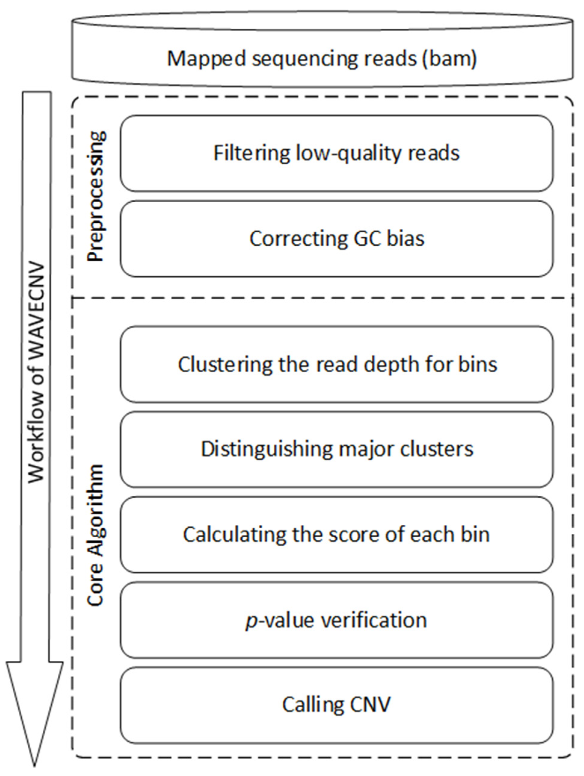
2.1. Workflow of WAVECNV

RD is affected by many artifacts, including sequencing error, repeatability of reads, and GC bias, which will lead to the uneven distribution of reads mapped in the reference genome. WAVECNV infers CNV by RD values in a single sample without control-matched samples. WAVECNV accepts alignment files stored in BAM format as input, which is usually aligned by BWA [18] software. Based on the BAM file, WAVECNV detects CNV through the following five processes, as shown in Figure 1: (1) Preprocessing: In this step, we discard the positions of “N” in the reference genome, every 1000 bases are considered as a bin, and the RD of each bin are counted. Then, the total number of bases “G” and “C” are counted in each bin, and GC bias correction is performed [19]. (2) Clustering the RDs of bins by wavelet clustering: In this step, we use the wavelet clustering method to cluster all the bins. The center position and average RD of clustering results are also recorded. (3) Distinguishing normal and abnormal clusters: In this step, several clusters with the largest number of bins are taken as the main clusters, and the number of bins in these main clusters should reach 80% of the total number. (4) Calculating the scores of each bin: In this step, the relative distance between each bin and the normal cluster is used as one of the important basis for scoring. Then, we use the logarithmic function to eliminate the imbalance between the amplitudes of missing and repeated segments. (5) Calling CNVs by p-value verification: In this step, we use the p-value to predict CNVs according to the distribution of scores. The complete method process is published at https://github.com/BDanalysis/waveCNV (accessed on 30 May 2022).

2.2. Preprocessing

In this stage, we used the widely effective methods in prior research for reference [20], filtered the invalid data in the gene, counted the RDs, and corrected the GC bias. Firstly, the “N” positions were removed from the reference genome. Secondly, the starting positions of reads were obtained from the BAM file, and the number of reads on 1000 consecutive bases was recorded as the RD of each bin. Finally, the GC deviation was corrected according to the ratio of bases “G” and “C” in each bin [19].

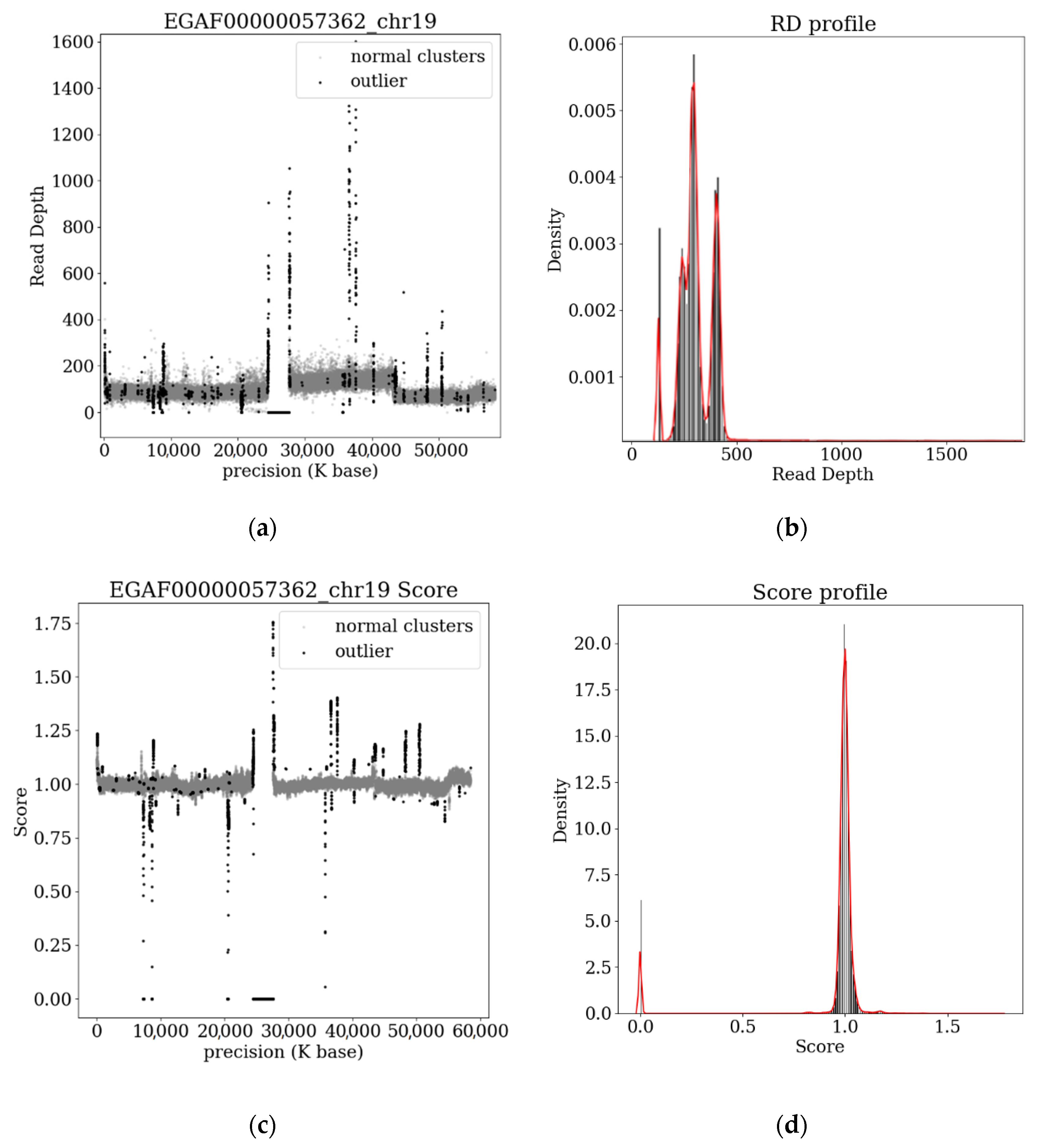
2.3. Clustering the RDs of Bins by Wavelet Clustering

In the clustering stage, we considered that each bin has its RD and position, so the basis of clustering should comprehensively consider these two features. We used Wavelet Cluster instead of the segmentation function of CBS. Compared with CBS, wavelet clustering can preserve the characteristics of small segment variation [14]. These preserved small segment variation characteristics help us find the variation area that is ignored by the CBS method. Wavelet clustering determines different clusters through the density relationship of data in a grid. The parameters of wavelet clustering control the number of units to segment data, and the number of clusters is not required as parameter input. We chose the same cluster with a density error of less than 1% by controlling the threshold to merge clusters with similar densities. Finally, we obtained the final clustering result. The detailed steps of wavelet clustering are described in the Supplementary Materials.

2.4. Distinguishing Normal and Abnormal Clusters

According to Richard Redon’s study, CNVs only account for 12~16% of the whole genome [2], but due to the influence of tumor purity, this ratio fluctuates for each sample. As an “abnormality” in gene duplication, the length of copy number variants should be smaller than the length of normal genes. However, there are cases where the length of the copy number variation is greater than 20% of the total length. For these individual cases, we use the threshold $\mathsf{\delta }$ as an input parameter; on the one hand, we believe that the normal gene length will not be less than 50% of the total length, and on the other hand, the variation of this threshold has little effect on the results, and we set the default value to 80%. The selection process of normal clusters is as follows: (1) The clustering results were sorted according to the number of bins to generate sequence C, and (2) the number of bins of the first m clusters in sequence C was summed. If the sum of bins was greater than $\mathsf{\delta }$ of the total number, the first m clusters were regarded as normal clusters.

2.5. Calculating the Scores of Each Bin

To correctly measure the outlier degree of each bin, it is necessary to calculate the distance between a bin and its nearest normal cluster. Each bin generally has two attributes: its RD and position. Therefore, we use $\left(r_i,p_i\right)$ to describe a bin, where $r_i$ and $p_i$ represent the RD and the position of the i-th bin, respectively. Similarly, for the j-th cluster, there are two attributes: average RD and center position, which are represented by $\left({\overline{R}}_j,{\overline{P}}_j\right)$.

The calculation formula for outlier degree is as follows:

$$D\left(i\right)=\underset{1\le j\le m}{\min }\left[{\left(r_i-{\overline{R}}_j\right)}^2+{\left(p_i-{\overline{P}}_j\right)}^2\right]$$

(1)

where D(i) represents the distance between the i-th bin and the nearest normal cluster.

$$S\left(r_i\right)=\frac{{\log }_2\left(r_i+1\right)}{{\log }_2\left(\overline{R}+1\right)}$$

(2)

where $S\left(r_i\right)$ represents the score of each bin, $r_i$ is the RD of i-th bin, and $\overline{R}$ represents the average RD of the normal cluster closest to the i-th bin. Scoring each bin relative to the nearest normal cluster through Formula (2) can eliminate the problem of uneven RDs caused by sequencing errors and repeated reads and reduce the imbalance of the amplitudes of CNVs between duplication and deletion.

The relationship between RD and location is shown in Figure 2a, and RD distribution is shown in Figure 2b. The relationship between the score and position according to Formula (2) is shown in Figure 2c, and the score distribution is shown in Figure 2d.

2.6. Calling CNVs by p-Value Verification

Since the distribution varies between samples, it is not reasonable to manually define an appropriate cutoff value for each sample. Nevertheless, in statistical hypothesis testing, a commonly used value can be assigned to the significance level. We assume that the outlier score obtained by RDs through formula (2) fits the normal distribution. Then, the statistical hypothesis test procedure was used to evaluate the significance of each abnormal bin. Considering the ability to detect variation in both duplication and deletion, we used the p-value of the two-sided test as the criterion for calling CNV (i.e., $P=P\left\{\left|X\right|>C\right\} ,\alpha =0.01$).

After determining the CNV areas by p-value [21], it is necessary to determine the variant type of the areas and calculate the corresponding CN. We used the classical calculation method to estimate the absolute copy number of the current fragment based on tumor purity, ploidy, and average RD [22]. The specific formula is as follows:

$$\mathrm{CN}=\frac{\left(r_t-\left(1-\phi \right)·r_n\right)·\rho }{\phi ·r_n}$$

(3)

where $r_t$ represents the average RD of CNV fragments, $r_n$ represents the average RD of normal fragments, $\rho$ represents tumor ploidy, and $\phi$ represents tumor purity.

3. Results

The evaluation and comparison of performance with existing methods is an important step to verify the accuracy and universality of an algorithm. To compare the performance of WAVECNV and other existing methods, we used IntSiM to generate 140 simulation data with different purity and coverage. The precision, sensitivity, and F1 score of CNV detection methods with different purity and coverage were compared between WAVECNV and five existing methods (CNVnator, CNVkit, FREEC, CNV-IFTV, and icopydav). We also used real data to compare the six methods. The real data come from the EGA database [23], which records the gene sequencing files of a large number of cancer samples. We used five samples from the lung cancer dataset numbered EGAD00000100144. The sequencing data of these five samples are whole-genome sequencing data from different patients with average coverage ranging from 5× to 12×. It is able to represent most of the possible scenarios in human genomic cancer-sequencing data.

The test results show the CNV overlaps detected among the six methods, and the detection results were compared with the cancer genes in the cancer gene census (CGC) [24]. We compared the number of cancer genes that could be detected by the six methods.

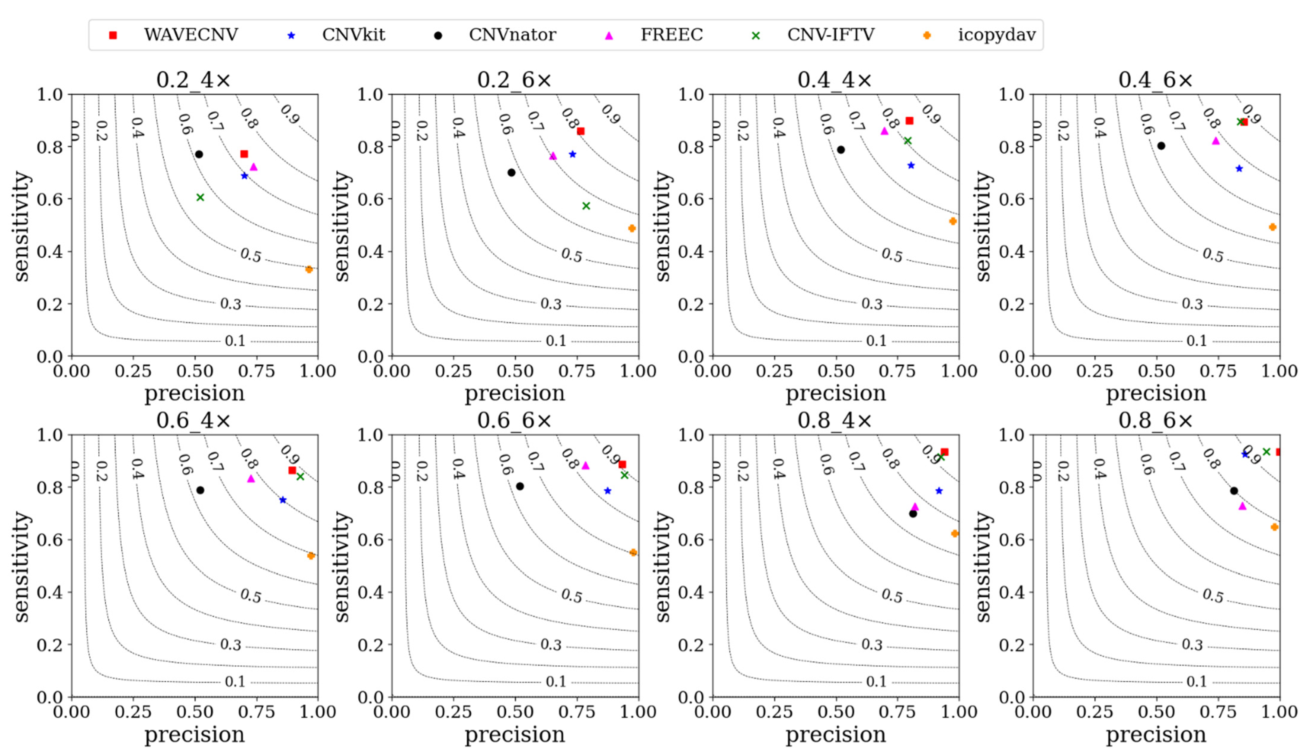
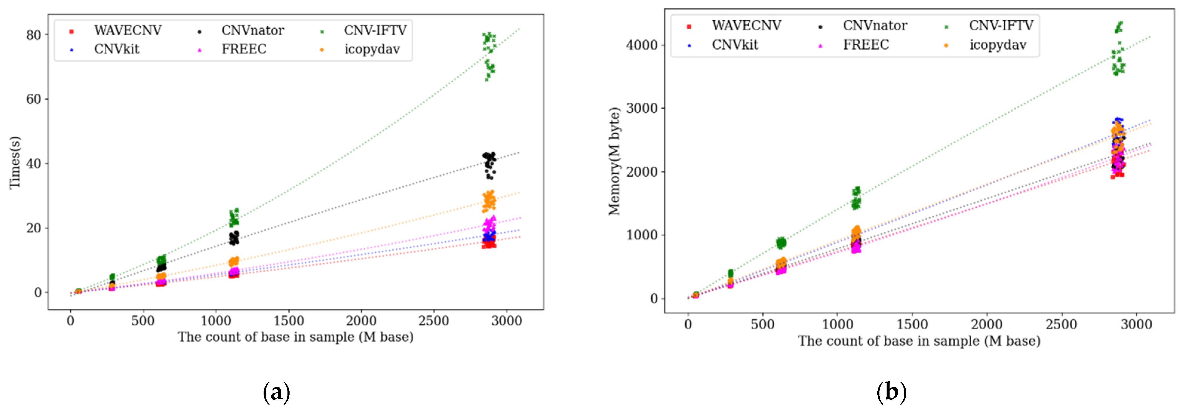
3.1. Simulation Studies

IntSIM [25] software can generate simulated data with different purity and coverage according to the parameters. The simulation data used in the experiment have tumor purity from 0.2 to 0.8 and coverage of 4× and 6×. The simulation data contain 10 CNV regions with length ranging from 5 kb to 50 kb. The precision and sensitivity of the compared six methods in different purity and coverage data are shown in Figure 3. Among the six methods, WAVECNV has the highest sensitivity in all tumor purity and sequencing coverage configurations, which shows that wavelet clustering can effectively retain the shorter CNV fragments in the RD data. Therefore, the sensitivity of WAVECNV to variation fragments is higher than that of the other five methods. Considering the balance between precision and sensitivity, the F1 scores of six methods are also calculated, among which WAVECNV has the highest F1 scores in all of the configurations. Only in high-purity and high-coverage data were some of the methods able to achieve the same precision and sensitivity as WAVECNV.

In addition, we use the above six methods to detect the simulation data with noise, and WAVECNV still has good performance. The detailed test results are shown in the Supplementary Materials.

We also compared the time and memory consumed by the whole process of six methods in processing these simulation data. We designed input files of different sizes according to different lengths of chromosomes and counted the time and memory used by the six methods in processing these files. According to Figure 4, in terms of computing time, WAVECNV, FREEC, iCopyDav, and CNVkit methods use the shortest time. The time used by WAVECNV is the same as that of the fastest method, CNVkit. Both CNVnator and CNV-IFTV methods consumed a long time. The comparison of memory usage shows that except for CNVkit, the memory usage of other methods is not much different.

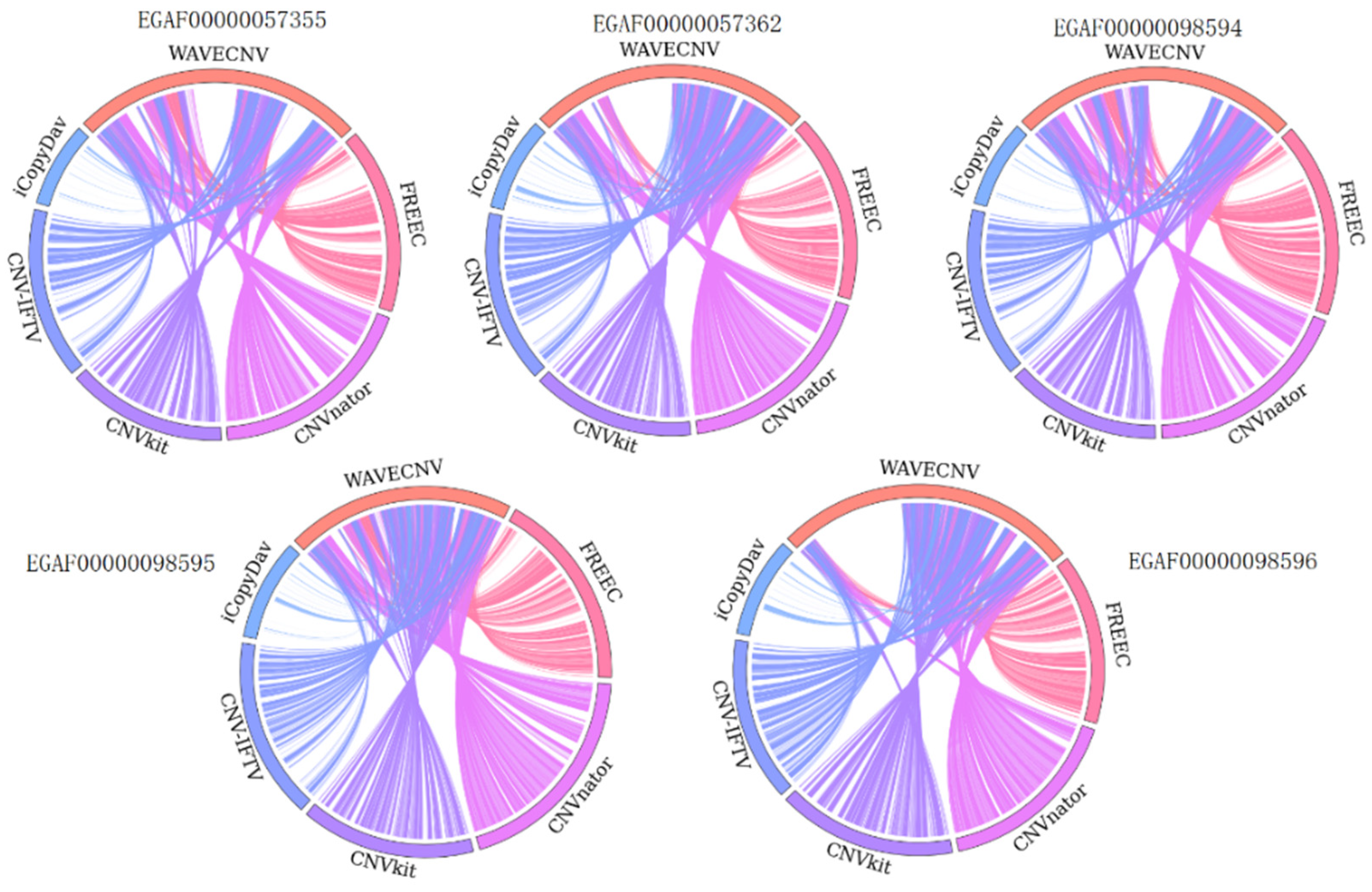
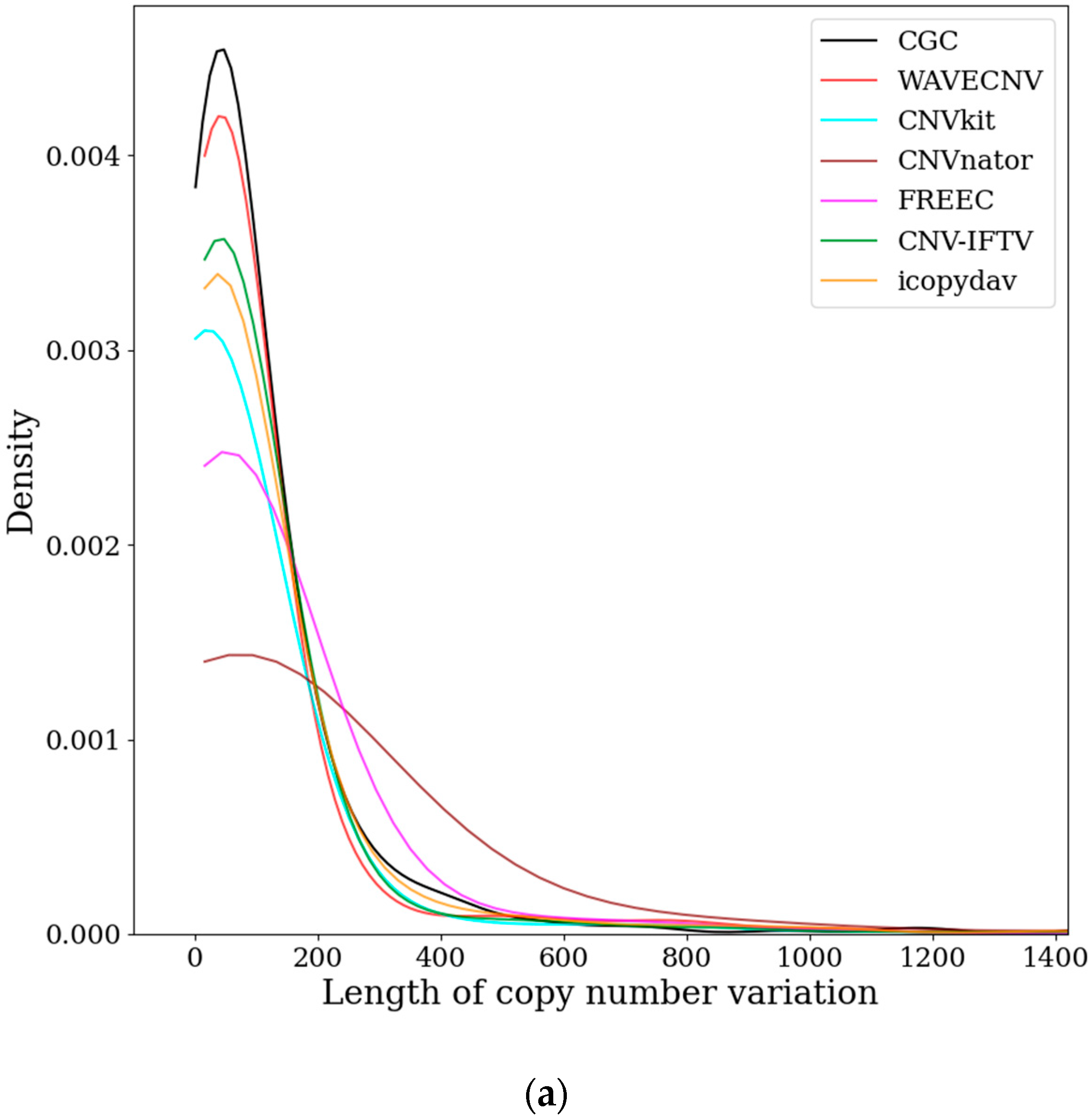
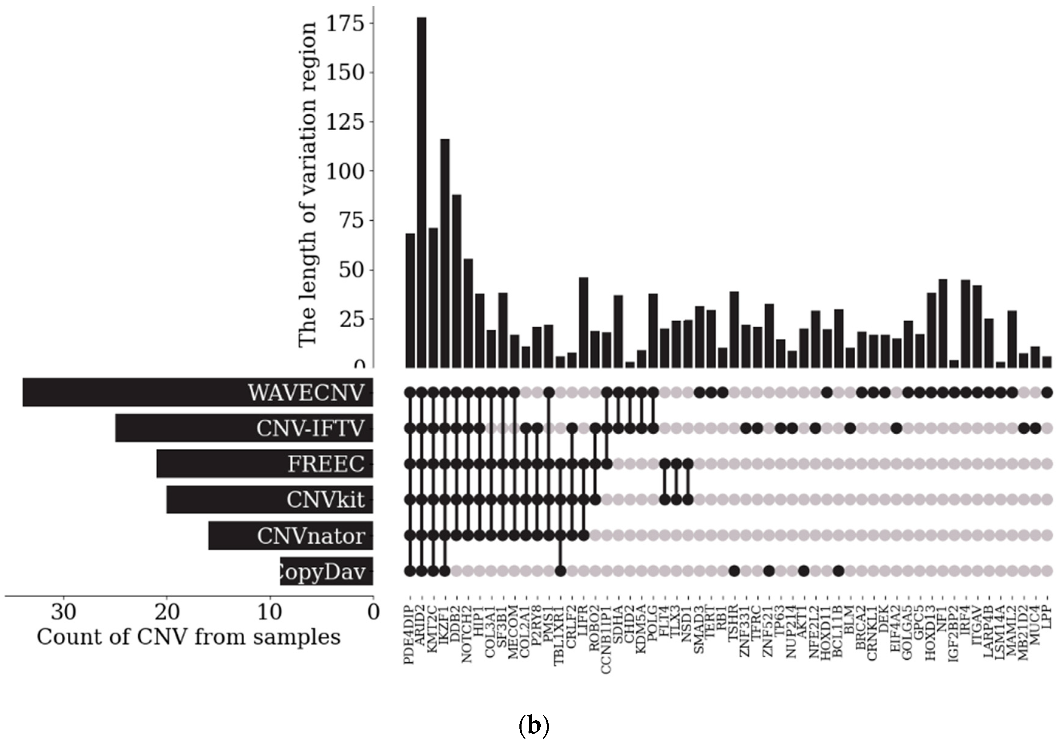
3.2. Analysis of Samples from the EGA

In addition to simulation data, the application of our proposed method to real data is equally important, and we used five samples from the lung cancer dataset EGAD0000100144 to compare the six methods. The five samples are EGAF00000057355, EGAF00000057362, EGAF00000098594, EGAF00000098595, and EGAF00000098596. The comparison results of the six methods are shown in Figure 5. It can be seen that WAVECNV has the widest coverage of the CNV region and can detect the most CNV regions compared to other methods. We also compared the detection results with the cancer genes published by the CGC, retained the overlapping parts of the detection results with the cancer gene positions published in the CGC, and compared the length distribution of the overlapping sections. As can be seen from the curve in Figure 6a, the copy number length detected by WAVECNV is closest to the CGC gene length distribution. In further depth, the number of cancer genes detected by the six methods, the length of overlapping segments, and the names of cancer genes detected by each method can be seen in Figure 6b. Figure 6b shows that WAVECNV detected the most cancer variant segments. The four cancer genes with long variant segments can be detected by all six methods, and WAVECNV can detect other shorter variant segments overlapping the cancer gene. This shows that WAVECNV can find some new short-length variant regions in the detection of CNV in cancer samples.

4. Discussion

This study proposes a new method for detecting CNV based on single-NGS samples. The method uses wavelet clustering and distance-based scoring, which on one hand ensures high-resolution clustering results and on other hand uses distance features to filter out the noise generated by clustering, thus ensuring the accuracy of variant fragments. Compared with other existing methods, WAVECNV has the following advantages: (1) Wavelet clustering has higher resolution and can keep the detailed information of RD data. This means that the deletion fragments in RD with smaller magnitudes can be distinguished with wavelet clustering. (2) The distance-based scoring method can estimate the outlier degree of the bin according to the RD difference between the bin and the normal segment. That is, this method greatly reduces the impact of unbalanced RDs in sequencing data on the detection results. (3) Using wavelet clustering to deal with RD data requires fewer parameters, which can avoid the uncertain influence of too many parameters on the variation result of copy number.

Through experiments with a large number of simulated data and real data, we compared the precision, sensitivity, and F1-score of WAVECNV and the existing five methods. WAVECNV has the best sensitivity and F1 score, and in the calculation process, it takes a short time and occupies a small memory. From the results of real data, WAVECNV can accurately detect the position of CNV and detect many neglected CNV fragments in real lung cancer data.

About work for future improvements, we plan to improve the function of WAVECNV and open the input of some optional parameters so that users can more flexibly control the precision of CNV-detection results [26]. We will use additional information from the sequencing data, such as variant allele frequency (VAF) [27,28], to more accurately estimate tumor purity and absolute copy number. In addition, we will develop a multi-sample CNV-detection method of WAVECNV to study the changes in the absolute copy number of genes in cancer patients at different periods [9] and lay a solid foundation for the inference of tumor subclonal populations.

References

1. Handsaker, R.E.; Doren, V.V.; Berman, J.R.; Genovese, G.; Kashin, S.; Boettger, L.M.; McCarroll, S.A. Large multiallelic copy number variations in humans. Nat. Genet. 2015, 47, 296–303. [Google Scholar] [CrossRef] [Green Version]
2. Redon, R.; Ishikawa, S.; Fitch, K.; Feuk, L.; Perry, G.; Andrews, T.; Fiegler, H.; Shapero, M.; Carson, A.; Chen, W.; et al. Global variation in copy number in the human genome. Nature 2006, 444, 444–454. [Google Scholar] [CrossRef] [PubMed] [Green Version]
3. Metzker, M.L. Sequencing technologies—The next generation. Nat. Rev. Genet. 2010, 11, 31–46. [Google Scholar] [CrossRef] [PubMed] [Green Version]
4. Mao, Y.-F.; Yuan, X.-G.; Cun, Y.-P. A novel machine learning approach (svmSomatic) to distinguish somatic and germline mutations using next-generation sequencing data. J. Zool. Res. 2021, 42, 246–249. [Google Scholar] [CrossRef]
5. Tarabichi, M.; Salcedo, A.; Deshwar, A.G.; Ni Leathlobhair, M.; Wintersinger, J.; Wedge, D.C.; Van Loo, P.; Morris, Q.D.; Boutros, P.C. A practical guide to cancer subclonal reconstruction from DNA sequencing. Nat. Methods 2021, 18, 144–155. [Google Scholar] [CrossRef] [PubMed]
6. Olshen, A.B.; Venkatraman, E.S.; Lucito, R.; Wigler, M. Circular binary segmentation for the analysis of array-based DNA copy number data. Biostatistics 2004, 5, 557–572. [Google Scholar] [CrossRef] [PubMed]
7. Prashanthi, D.; Sriharsha, V.; Nita, P.; Ulrich, M.J.P.O. iCopyDAV: Integrated platform for copy number variations—Detection, annotation and visualization. PLoS ONE 2018, 13, e0195334. [Google Scholar]
8. Talevich, E.; Shain, A.H.; Botton, T.; Bastian, B.C. CNVkit: Genome-Wide Copy Number Detection and Visualization from Targeted DNA Sequencing. PLoS Comput. Biol. 2016, 12, e1004873. [Google Scholar] [CrossRef]
9. Zaccaria, S.; Raphael, B.J. Accurate quantification of copy-number aberrations and whole-genome duplications in multi-sample tumor sequencing data. Nat. Commun. 2020, 11, 4301. [Google Scholar] [CrossRef]
10. Yuan, X.; Yu, J.; Xi, J.; Yang, L.; Shang, J.; Li, Z.; Duan, J. CNV_IFTV: An isolation forest and total variation-based detection of CNVs from short-read sequencing data. IEEE/ACM Trans. Comput. Biol. Bioinform. 2019, 18, 539–549. [Google Scholar] [CrossRef]
11. Abyzov, A.; Urban, A.E.; Snyder, M.; Gerstein, M.J.G.R. CNVnator: An approach to discover, genotype, and characterize typical and atypical CNVs from family and population genome sequencing. Genome Res. 2011, 21, 974–984. [Google Scholar] [CrossRef] [PubMed] [Green Version]
12. Comaniciu, D.; Meer, P. Mean shift: A robust approach toward feature space analysis. IEEE Trans. Pattern Anal. Mach. Intell. 2002, 24, 603–619. [Google Scholar] [CrossRef] [Green Version]
13. Yuan, X.; Li, J.; Bai, J.; Xi, J. A Local outlier factor-based detection of copy number variations from NGS data. IEEE/ACM Trans. Comput. Biol. Bioinform. 2019, 18, 1811–1820. [Google Scholar] [CrossRef] [PubMed]
14. Lai, W.R.; Johnson, M.D.; Kucherlapati, R.; Park, P.J. Comparative analysis of algorithms for identifying amplifications and deletions in array CGH data. Bioinformatics 2005, 21, 3763–3770. [Google Scholar] [CrossRef] [PubMed] [Green Version]
15. Sheikholeslami, G.; Chatterjee, S.; Zhang, A. WaveCluster: A wavelet-based clustering approach for spatial data in very large databases. VLDB J. 2000, 8, 289–304. [Google Scholar] [CrossRef]
16. Liu, F.T.; Ting, K.; Zhou, Z.-H. Isolation Forest. In Proceedings of the 2008 Eighth IEEE International Conference on Data Mining, Pisa, Italy, 15–19 December 2008; pp. 413–422. [Google Scholar] [CrossRef]
17. Boeva, V.; Popova, T.; Bleakley, K.; Chiche, P.; Cappo, J.; Schleiermacher, G.; Janoueix-Lerosey, I.; Delattre, O.; Barillot, E.J.B. Control-FREEC: A tool for assessing copy number and allelic content using next-generation sequencing data. Bioinformatics 2011, 28, 423–425. [Google Scholar] [CrossRef]
18. Li, H.; Durbin, R. Fast and accurate short read alignment with Burrows–Wheeler transform. Bioinformatics 2009, 25, 1754–1760. [Google Scholar] [CrossRef] [Green Version]
19. Benjamini, Y.; Speed, T.P. Summarizing and correcting the GC content bias in high-throughput sequencing. Nucleic Acids Res. 2012, 40, e72. [Google Scholar] [CrossRef] [Green Version]
20. Miller, C.A.; Hampton, O.; Coarfa, C.; Milosavljevic, A. ReadDepth: A parallel r package for detecting copy number alterations from short sequencing reads. PLoS ONE 2011, 6, e16327. [Google Scholar] [CrossRef] [Green Version]
21. Yu, Z.; Li, A.; Wang, M. CloneCNA: Detecting subclonal somatic copy number alterations in heterogeneous tumor samples from whole-exome sequencing data. BMC Bioinform. 2016, 17, 310. [Google Scholar] [CrossRef] [Green Version]
22. Poell, J.B.; Mendeville, M.; Sie, D.; Brink, A.; Brakenhoff, R.H.; Ylstra, B.J.B. ACE: Absolute copy number estimation from low-coverage whole-genome sequencing data. Bioinformatics 2019, 35, 2847–2849. [Google Scholar] [CrossRef] [PubMed]
23. Freeberg, M.A.; Fromont, L.A.; D’Altri, T.; Romero, A.F.; Ciges, J.I.; Jene, A.; Kerry, G.; Moldes, M.; Ariosa, R.; Bahena, S.; et al. The European Genome-phenome Archive in 2021. Nucleic Acids Res. 2021, 50, D980–D987. [Google Scholar] [CrossRef] [PubMed]
24. Sondka, Z.; Bamford, S.; Cole, C.G.; Ward, S.A.; Dunham, I.; Forbes, S.A. The COSMIC Cancer Gene Census: Describing genetic dysfunction across all human cancers. Nat. Cancer 2018, 18, 696–705. [Google Scholar] [CrossRef]
25. Yuan, X.; Zhang, J.; Yang, L. IntSIM: An Integrated Simulator of Next-Generation Sequencing Data. IEEE Trans. Biomed. Eng. 2016, 64, 441–451. [Google Scholar] [CrossRef]
26. Chen, Y.; Zhao, L.; Wang, Y.; Cao, M.; Gelowani, V.; Xu, M.; Agrawal, S.A.; Li, Y.; Daiger, S.P.; Gibbs, R.; et al. SeqCNV: A novel method for identification of copy number variations in targeted next-generation sequencing data. BMC Bioinform. 2017, 18, 147. [Google Scholar] [CrossRef] [Green Version]
27. Cmero, M.; Yuan, K.; Ong, C.S.; Schröder, J.; Adams, D.J.; Anur, P.; Beroukhim, R.; Boutros, P.C.; Bowtell, D.D.L.; Campbell, P.J.; et al. Inferring structural variant cancer cell fraction. Nat. Commun. 2020, 11, 730. [Google Scholar] [CrossRef] [PubMed] [Green Version]
28. Deshwar, A.G.; Vembu, S.; Yung, C.K.; Jang, G.H.; Stein, L.; Morris, Q. PhyloWGS: Reconstructing subclonal composition and evolution from whole-genome sequencing of tumors. Genome Biol. 2015, 16, 35. [Google Scholar] [CrossRef] [Green Version]
Figure 1. The workflow of WAVECNV.
Mathematics 10 02151 g001
Figure 2. The clustering result of chromosome 19 in sample EGAF00000057362. (a) RD–position diagram shows the RD of each bin. The gray dots represent the bins in the normal cluster, and the black dots represent the bins in the abnormal cluster, also known as an outlier. (b) RD vs. frequency distribution curve. (c) This chart shows the score of each bin, in which the uneven RDs have been corrected. (d) Fractional frequency distribution diagram. By correcting the uneven RDs and unbalanced amplitudes, the normal distribution is able to fit the scores of all bins.
Mathematics 10 02151 g002
Figure 3. The precision, sensitivity, and F1 scores of the six methods are compared in the simulation data with different coverage and purity. The dotted line in the figure represents the contour line of the F1 score, the decimal of the title in the figure represents the tumor purity, and 4× and 6× represent 4 or 6 times the coverage. Among them, WAVECNV has the highest sensitivity and highest precision.
Mathematics 10 02151 g003
Figure 4. The figure shows the time and memory used by the six methods to call CNVs in the simulated data with the coverage of 8×. (a) The trend of algorithm calculation time with the count of bases in a sample. (b) Relationship between the size of memory and the count of bases in a sample.
Mathematics 10 02151 g004
Figure 5. The length of the circle in the figure represents the total length of CNV detected by the six methods, and the connecting line in the circle represents the same CNV region detected by different methods.
Mathematics 10 02151 g005
Figure 6. (a) The black curve represents the length distribution of cancer genes published by CGC. The red curve represents the length distribution coinciding with the cancer gene fragment in the WAVECNV test results. The curves of other colors represent the length distribution of the detection results of the remaining five methods coinciding with the cancer gene fragment. (b) The histogram at the top of the figure represents the length of cancer genes, and the bar chart at the left of the figure represents the number of cancer genes in the results of the six methods. The dot graph at the bottom right of the figure represents the cancer gene fragments detected by the six methods. Black dots represent the fragments that can be detected by this method, and gray dots represent the fragments that are not detected by this method.
Mathematics 10 02151 g006aMathematics 10 02151 g006b
Publisher’s Note: MDPI stays neutral with regard to jurisdictional claims in published maps and institutional affiliations.