Convergence Behavior of Optimal Cut-Off Points Derived from Receiver Operating Characteristics Curve Analysis: A Simulation Study

Abstract

The area under the receiver operating characteristics curve is a popular measure of the overall discriminatory power of a continuous variable used to indicate the presence of an outcome of interest, such as disease or disease progression. In clinical practice, the use of cut-off points as benchmark values for further treatment planning is greatly appreciated, despite the loss of information that such a dichotomization implies. Optimal cut-off points are often derived from fixed sample size studies, and the aim of this study was to investigate the convergence behavior of optimal cut-off points with increasing sample size and to explore a heuristic and path-based algorithm for cut-off point determination that targets stagnating cut-off point values. To this end, the closest-to-(0,1) criterion in receiver operating characteristics curve analysis was used, and the heuristic and path-based algorithm aimed at cut-off points that deviated less than 1% from the cut-off point of the previous iteration. Such a heuristic determination stopped after only a few iterations, thereby implicating practicable sample sizes; however, the result was, at best, a rough estimate of an optimal cut-off point that was unbiased and positively and negatively biased for a prevalence of 0.5, smaller than 0.5, and larger than 0.5, respectively.

1. Introduction

The search for biomarkers that indicate a clinical outcome of interest (such as disease presence or recurrence) has been an incessant endeavor in medical research during the past decades. Several performance measures quantify a biomarker’s added value in predictive modeling, including both categorizing a continuous marker with cut-off points and using the whole of the information that a biomarker provides on a continuous scale [1]. The categorization of continuous variables has the advantage of straightforward implementation in clinical practice at the cost of information loss. The distance of a biomarker value to a given cut-off point may be small or large but still indicates the same classification of the subject, and functional relationships with the outcome of interest are easily disguised [2,3]. A clinical example is the Framingham Risk Score, used for estimating the 10-year cardiovascular risk of an individual, with low (less than 10%), moderate (10–19%), and high (20% or higher) risk categories [4,5,6]. Another example is the Agatston score for coronary calcification, which is classified, for instance, into 0, 1–9, 10–99, 100–399, and 400 or higher [7,8]. Based on the results of the Multi-Ethnic Study of Atherosclerosis, the Framingham Risk Score was extended using the Agatston score, illuminating the differences in the Framingham Risk Score when incorporating or disregarding the Agatston score for coronary calcification [9,10,11].

In diagnostic research, several criteria for cut-off point optimality have been proposed that are based on the receiver operating characteristics (ROC) curve [12,13]. The closest-to-(0,1) criterion [14] and the Youden index [15] indicate the optimal cut-off point as the one closest to perfect discrimination of subjects with or without the condition of interest and the point farthest from no discrimination, respectively [16]. Liu [17] introduced the concordance probability of the dichotomized measure at the optimal cut-off point, which geometrically represents the area of a rectangle below the ROC curve, with the optimal cut-off point as the top-left corner. In Stata, these three criteria are implemented in the command cutpt, with Liu’s method used as the default. Lopez-Raton et al. [18] introduced the R package OptimalCutpoints to select optimal cut-off points. They included criteria based on sensitivity and specificity (e.g., Youden index and closest-to-(0,1) criterion), predictive values, diagnostic likelihood ratios, cost–benefit analysis of the diagnosis, and maximum chi-squared or minimum p-value criterion.

In cancer research, first-in-human dose-finding trials aim to determine a maximal tolerable dose, which is associated with a probability of observing dose-limiting toxicity of 33%. Traditionally, the rule-based 3 + 3 design was used; nowadays, more efficient but computationally more demanding model-based (especially the continual reassessment method) and model-assisted (such as Bayesian optimal interval design) designs are employed [19,20,21].

This study aimed to transfer the idea of up-and-down designs in cancer dose-finding trials (such as the traditional 3 + 3 dose-escalation rule) to cut-off point-finding endeavors in diagnostic research. To achieve this, we investigated the convergence behavior of optimal cut-off points with increasing sample size in a simulation study and explored a heuristic and path-based algorithm for cut-off point determination that targeted stagnating cut-off point values.

2. Materials and Methods

2.1. Simulation Set-Up

The distribution of scores in subjects with (D1) and without (D0) a target condition can take very different forms. Hypothetical distributions employ normal distributions [12,13,22] and right-skewed distributions [23]. In practice, the abovementioned Agatston scores for coronary calcification are an example of a variable that often follows a right-skewed distribution, as the calcification scores are nonnegative integers, often with an overexpression of zeros in disease-free subjects [10,24]. Four sets of distributions were assumed for D0 and D1.

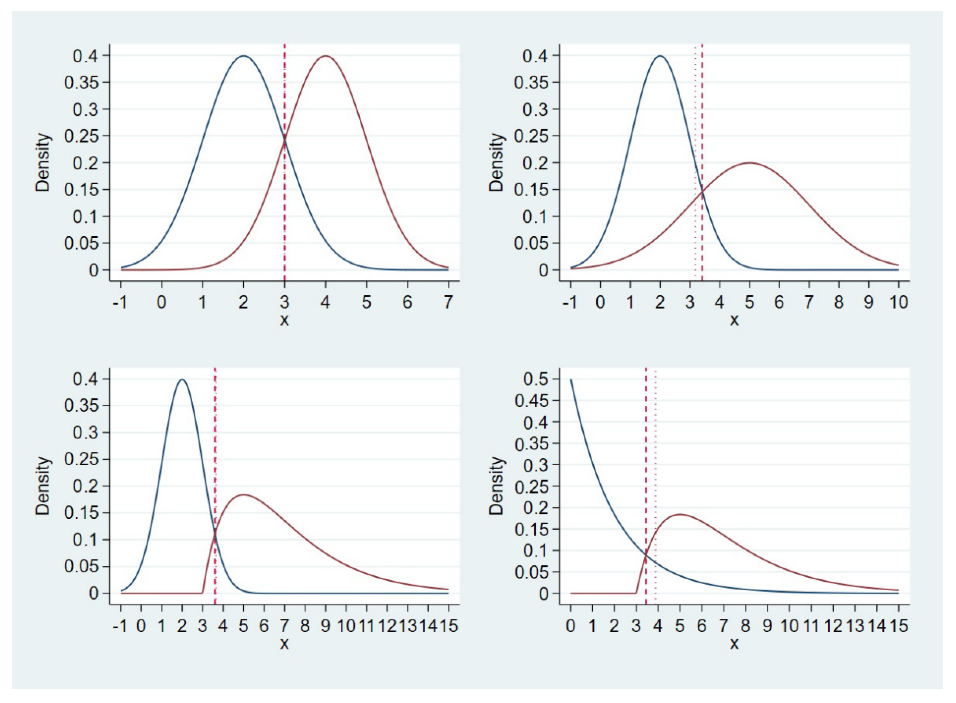
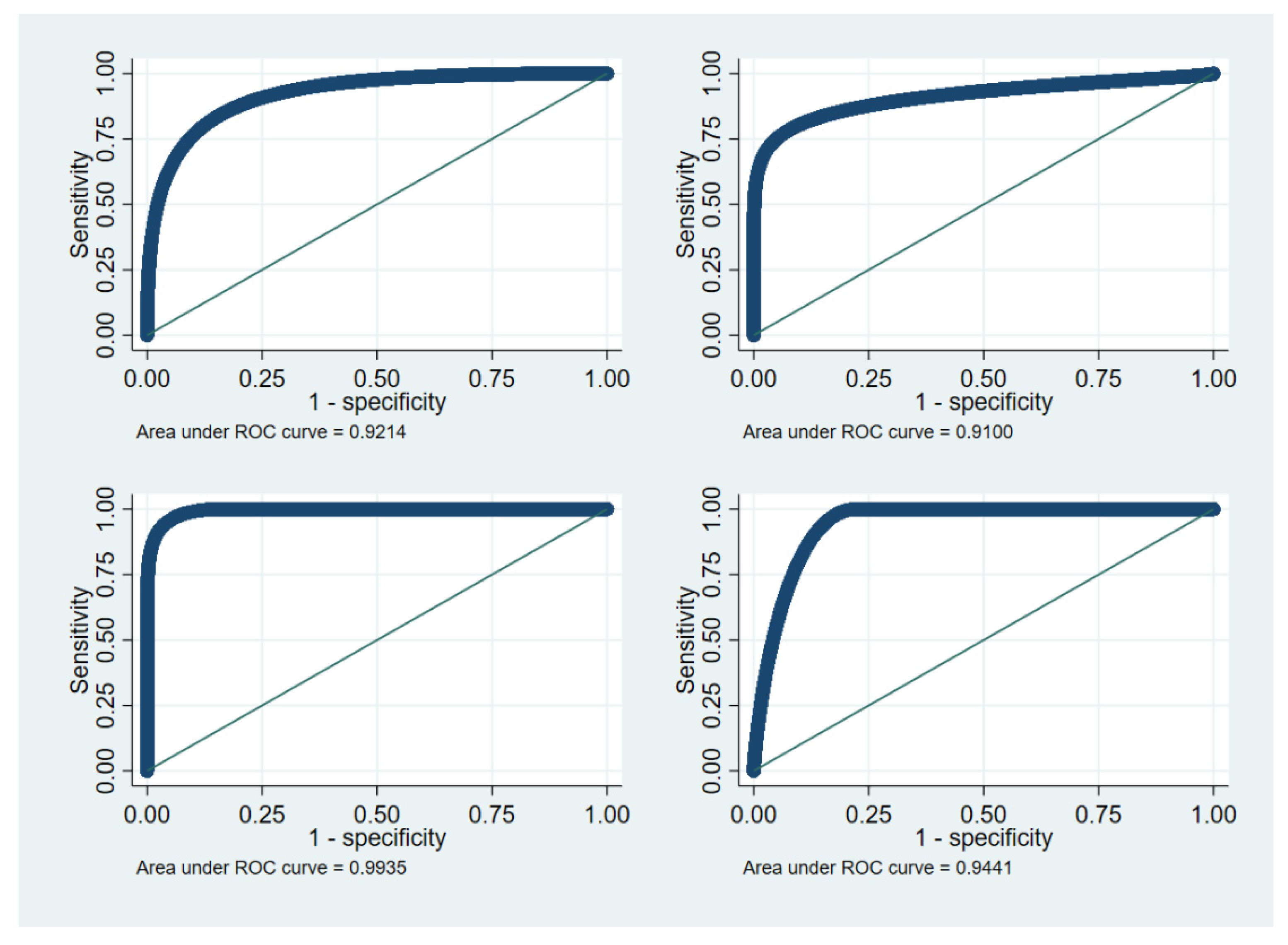
• Scenario 1: normal (mean = 2, variance = 1) and normal (mean = 4, variance = 1) for D0 and D1, respectively; top left corner of Figure 1;
• Scenario 2: normal (mean = 2, variance = 1) and normal (mean = 5, variance = 2) for D0 and D1, respectively; top right corner of Figure 1;
• Scenario 3: normal (mean = 2, variance = 1) and gamma (shape = 2, scale = 2, location = 3) for D0 and D1, respectively; bottom left corner of Figure 1;
• Scenario 4: exponential (scale = 2) and gamma (shape = 2, scale = 2, location = 3) for D0 and D1, respectively; bottom right corner of Figure 1.

Figure 1. Four sets of assumed distributions for D0 (left, blue line) and D1 (right, red line) subjects. Top left: scenario 1—normal (mean = 2, variance = 1) and normal (mean = 4, variance = 1). Top right: scenario 2—normal (mean = 2, variance = 1) and normal (mean = 5, variance = 2). Bottom left: scenario 3—normal (mean = 2, variance = 1) and gamma (shape = 2, scale = 2, location = 3). Bottom right: scenario 4—exponential (scale = 2) and gamma (shape = 2, scale = 2, location = 3). The vertical, dashed line indicates the optimal cut-off point according to the Youden index, which was 3, 3.42, 3.6, and 3.45 for scenarios 1–4, respectively. The vertical, dotted line indicates the optimal cut-off point according to the closest-to-(0,1) criterion, which was 3, 3.18, 3.65, and 3.88 for scenarios 1–4, respectively.

Figure 1. Four sets of assumed distributions for D0 (left, blue line) and D1 (right, red line) subjects. Top left: scenario 1—normal (mean = 2, variance = 1) and normal (mean = 4, variance = 1). Top right: scenario 2—normal (mean = 2, variance = 1) and normal (mean = 5, variance = 2). Bottom left: scenario 3—normal (mean = 2, variance = 1) and gamma (shape = 2, scale = 2, location = 3). Bottom right: scenario 4—exponential (scale = 2) and gamma (shape = 2, scale = 2, location = 3). The vertical, dashed line indicates the optimal cut-off point according to the Youden index, which was 3, 3.42, 3.6, and 3.45 for scenarios 1–4, respectively. The vertical, dotted line indicates the optimal cut-off point according to the closest-to-(0,1) criterion, which was 3, 3.18, 3.65, and 3.88 for scenarios 1–4, respectively.

The prevalence of the disease was assumed to be 0.1, 0.3, 0.5, and 0.7, and the number of simulated trials was 1000. An optimal cut-off point according to the closest-to-(0,1) criterion was determined with a minimum sample size of 100 to ensure a minimum of approximately 10 cases. We chose 101 subjects instead of 100 as the starting point to increase the chance of identifying a unique, optimal cut-off point; as the empirical ROC curve is a step function, cutpt may identify more than one closest-to-(0,1) cut-off point, leading to ties and termination of the procedure.

Reproducible Stata codes for all results are available in Supplementary Materials S1, and Stata data files, including optimal cut-off points by trial number and n = 101–801 in increments of 50 subjects, are available in Supplementary Materials S2. All analyses were performed using Stata/MP 17.0 (StataCorp, College Station, TX 77845 USA).

2.2. Criterion for Optimality of a Cut-Off Point

The Stata package cutpt enables cut-off point determination according to the Youden index, closest-to-(0,1) criterion, and Liu’s method. We employed the closest-to-(0,1) criterion because of its algorithmic stability when conducting the simulation study, as the non-identifiability of a unique optimal cut-off point, which leads to immediate termination of the algorithm, occurs less often with the closest-to-(0,1) criterion than with the other two methods.

2.3. True Optimal Cut-Off Points

With Se(c) and Sp(c) representing sensitivity (true-positives divided by the sum of true-positives and false-negatives) and specificity (true-negatives divided by the sum of true-negatives and false-positives), respectively, evaluated at cut-off point c, the optimal cut-off point is defined for each of these methods as follows [17]:

• Closest-to-(0,1) criterion:$c_{closest}=\underset{c}{\min }\sqrt{{\left[1-Se\left(c\right)\right]}^2+{\left[1-Sp\left(c\right)\right]}^2}$;
• Liu’s method:$c_{Liu}=\underset{c}{\max }\left(Se\left(c\right)Sp\left(c\right)\right)$;
• Youden index:$c_{Youden}=\underset{c}{\max }\left(Se\left(c\right)+Sp\left(c\right)-1\right)$.

As the assumed distributions for D0 and D1 are given (Figure 1), the true optimal cut-off points in scenarios 1–4 were evaluated by grid search (Supplementary Materials S1). For the closest-to-(0,1) criterion, the true optimal cut-off points were 3, 3.18, 3.65, and 3.88 for scenarios 1–4, respectively. Notably, the true optimal cut-off points were identical for the Youden index, closest-to-(0,1) criterion, and Liu’s method only for homoscedastic scenario 1, whereas these were different for the remaining heteroscedastic scenarios (

Table 1. True optimal cut-off points for all scenarios and closest-to-(0,1) criterion, Liu’s method, and Youden index.

Scenario	Closest-to-(0,1) Criterion	Liu’s Method	Youden Index
1	3	3	3
2	3.18	3.34	3.42
3	3.65	3.61	3.6
4	3.88	3.52	3.45

). Figure A1 depicts the respective ROC curves for all scenarios.

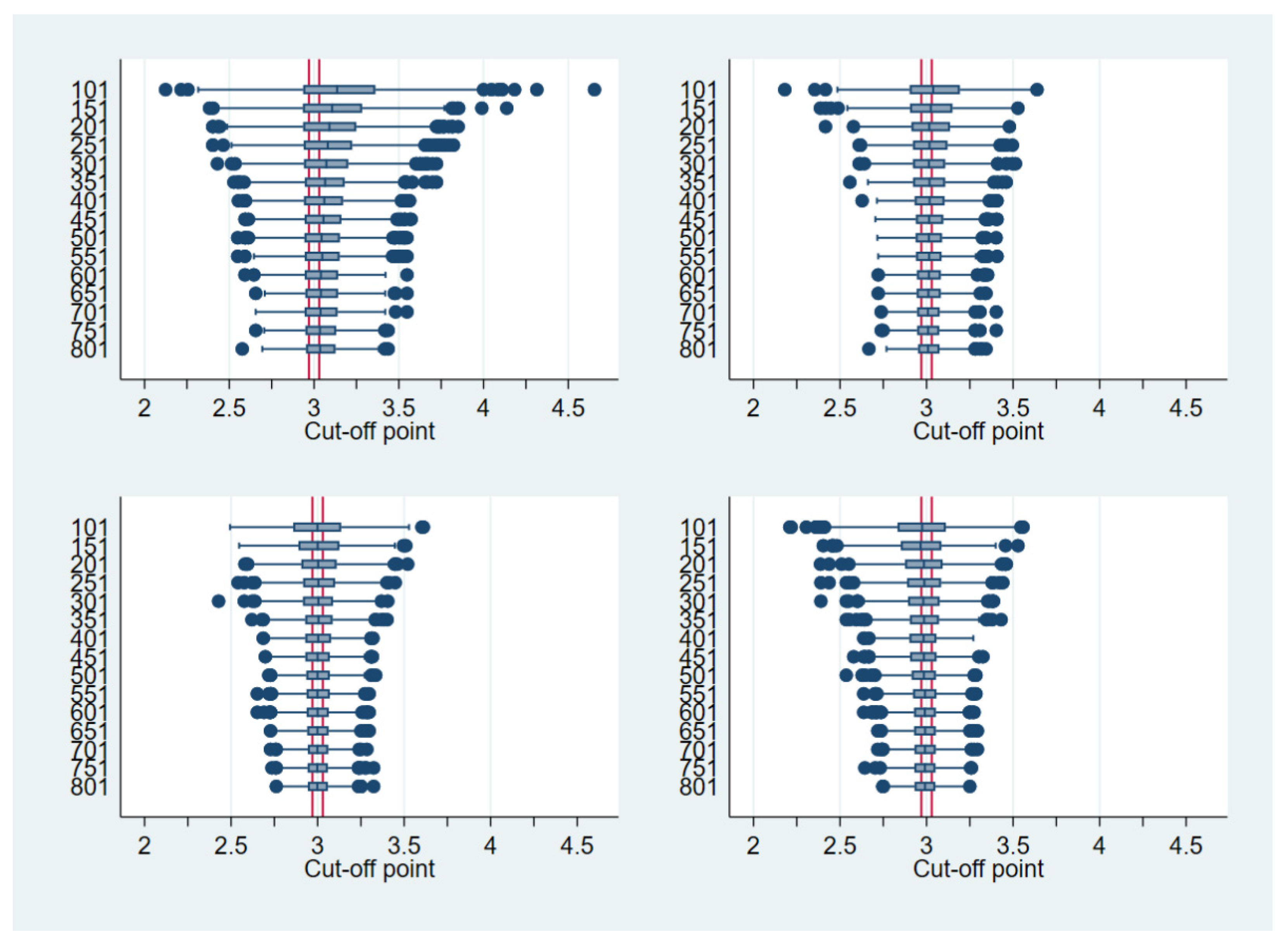
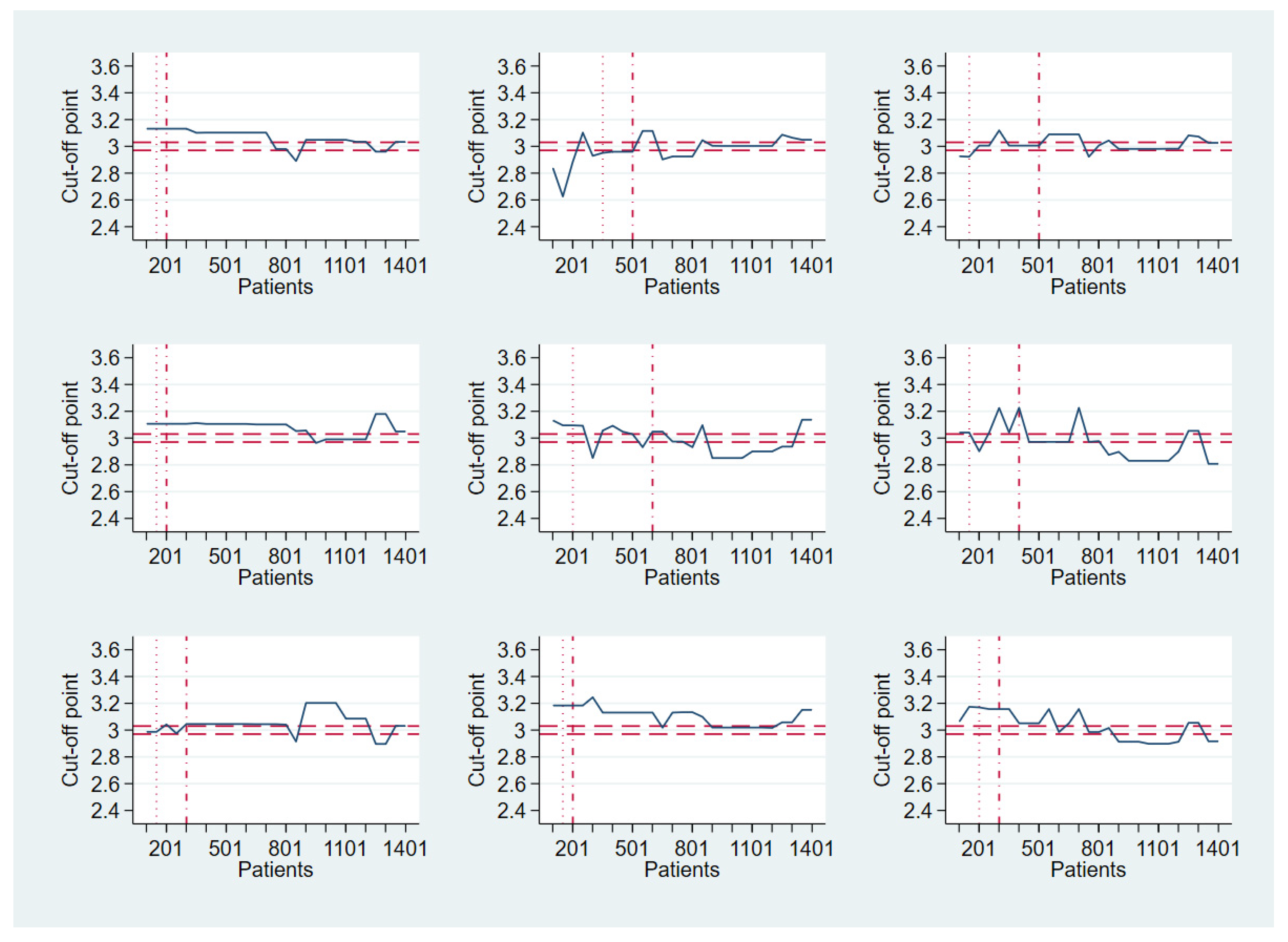
2.4. Convergence Behavior of Optimal Cut-off Points with Increasing Sample Size

For each setting and trial, the optimal cut-off points were determined for all sample sizes, n = 101, 151, 201, …, 801. For every estimated optimal cut-off point, the bias (in %) and mean squared error (MSE) in relation to the true values were derived. A bias smaller than a 1% deviation from the true optimal cut-off point was considered reasonably close to the true value. Boxplots demonstrate the location and skewness of the cut-off point distributions. Values larger than the third quartile plus 1.5 times the interquartile range and values smaller than the first quartile minus 1.5 times the interquartile range are shown individually, in accordance with the definition of boxplot outliers in Stata.

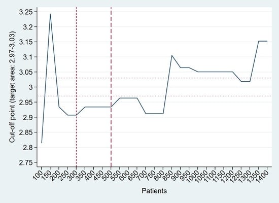
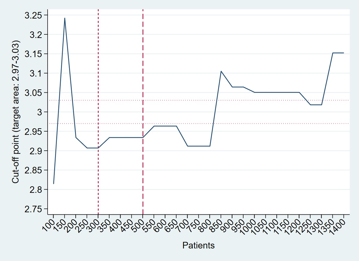
2.5. A Heuristic and Path-Based Algorithm for Cut-Off Point Determination

The optimal cut-off point estimate for ROC curves varies with increasing sample size and eventually converges to the true value. For each simulated trial, the search started with n = 101 subjects, and the cut-off point was estimated after increments of 50 (heuristic algorithm 1) and 100 (heuristic algorithm 2). The algorithm was stopped, and the cut-off point was identified when the estimated cut-off point deviated by less than 1% from the precedent estimate. To this end, the simulations in the previous section were used. The bias (in %) and MSE of the identified optimal cut-off points, as well as the mean number of patients and their respective 95% confidence intervals (95% CI), are reported.

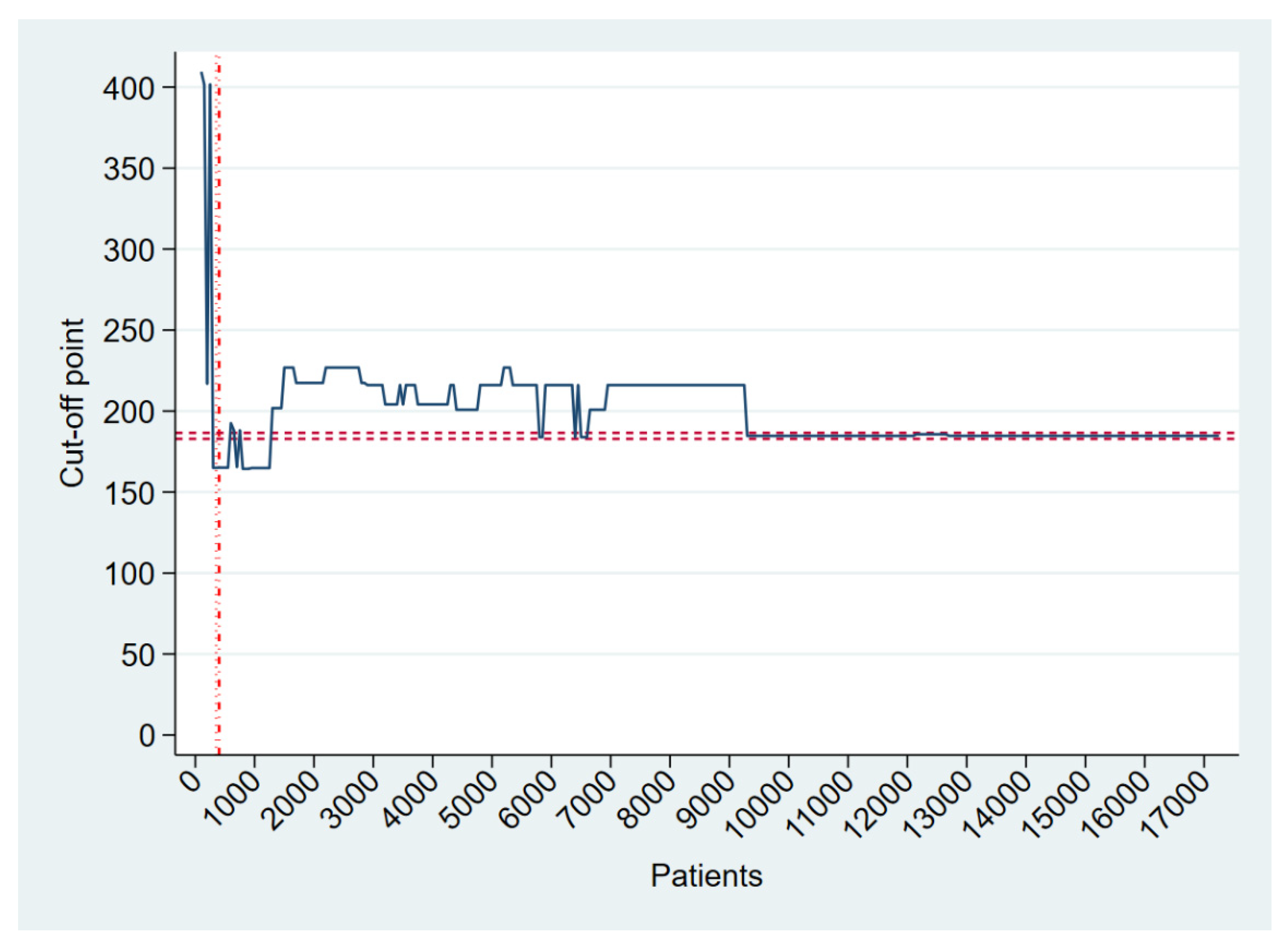
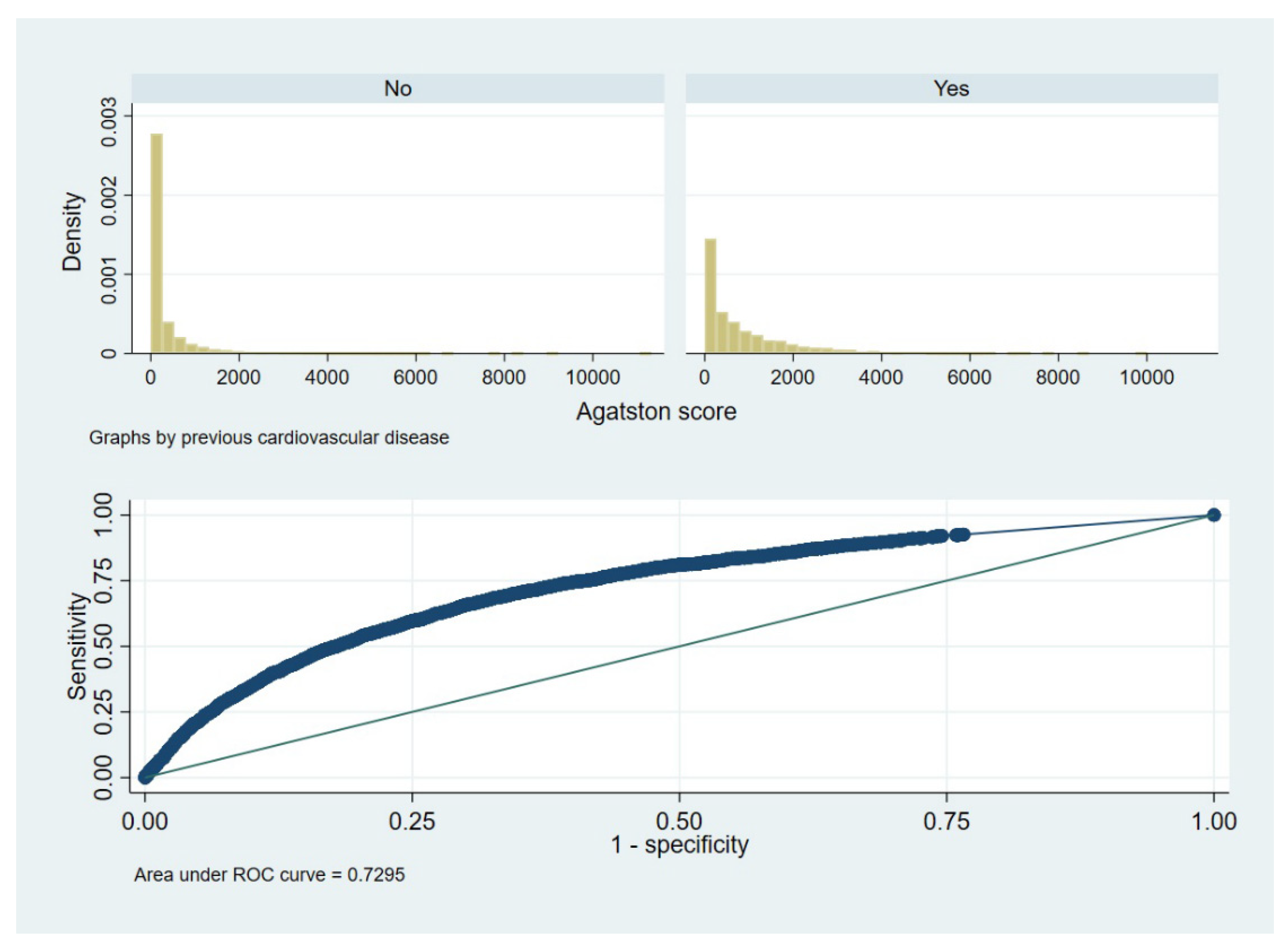
2.6. Real-Life Example Data

The Agatston score for coronary calcification is a nonnegative marker based on a coronary computed tomography (CT) scan. It is the total calcium score across all calcific lesions detected on slices obtained from the proximal coronary arteries [7]. The Agatston score has become a cardiovascular risk factor in addition to those previously known (male sex, age, smoking, systolic blood pressure, and total cholesterol) [25] and was measured as part of two population-based cardiac CT screening cohorts [26,27,28]. These Danish samples comprised 17,252 participants aged 50 to 75 years, among which 15% had a history of cardiovascular disease and 11.2% were female [24]. The data were randomly sorted by using 20,221,019 as seed.

The real-life example data are available in Supplementary Materials S4, and the Stata codes are part of Supplementary Materials S1.

3. Results

3.1. Fixed Sample Size

Figure 2 shows boxplots for optimal cut-off points for sample sizes n = 101, 151, 201, …, 801 and scenario 1 by prevalence. For a prevalence below 0.5, the optimal cut-off point was overestimated on average (Figure 2, top left corner: prevalence = 0.1; Figure 2, top right corner: prevalence = 0.3).

The smaller the prevalence, the higher the likelihood that sampling would include more D0 subjects in the tails of the distribution and, therefore, to the right of the true optimal cut-off point (see vertical, dashed, and dotted lines in Figure 1, top left corner). In contrast, sampling also included fewer D1 subjects in the tails of the distribution, leading to an overestimation of the estimated optimal cut-off point. With increasing sample size, the convergence of the estimate to the true optimal cut-off point was visible by means of narrower boxes (i.e., smaller interquartile ranges) around the true value of 3 (Figure 2). However, only for a prevalence of 0.5 (Figure 2, bottom left corner) did the first and third quartiles close onto the interval of 1% deviation from the true value, which was 2.97 to 3.03. The same was true for scenarios 2–4 (Supplementary Materials S3).

It was also only for a prevalence of 0.5 that the mean bias fell short of a 1% deviation from the true value across all four scenarios (

Table 2. Bias and mean squared error (MSE) of cut-off points in fixed sample designs.

Prevalence	Patients	Scenario 1		Scenario 2		Scenario 3		Scenario 4
		Bias, %	MSE	Bias, %	MSE	Bias, %	MSE	Bias, %	MSE
0.1	101	5.1	0.128	9.2	0.360	7.5	0.293	8.4	0.504
	201	3.4	0.068	4.7	0.154	4.5	0.130	5.8	0.242
	301	2.5	0.047	3.0	0.093	3.4	0.089	4.8	0.168
	401	1.9	0.034	2.7	0.074	2.9	0.065	3.8	0.122
	501	1.6	0.028	1.9	0.057	2.5	0.049	3.3	0.105
	601	1.4	0.023	1.5	0.044	2.1	0.038	2.8	0.085
	701	1.4	0.021	1.4	0.037	1.9	0.032	2.6	0.073
	801	1.3	0.018	1.5	0.033	1.7	0.028	2.2	0.061
0.3	101	1.5	0.045	1.7	0.098	1.8	0.069	2.7	0.169
	201	0.76	0.026	1.1	0.052	1.1	0.037	1.7	0.084
	301	0.63	0.019	0.90	0.035	0.98	0.026	1.2	0.064
	401	0.62	0.016	0.73	0.028	0.89	0.021	1.03	0.050
	501	0.50	0.012	0.60	0.023	0.81	0.017	1.01	0.043
	601	0.46	0.011	0.57	0.022	0.72	0.014	0.88	0.038
	701	0.38	0.010	0.61	0.019	0.62	0.013	0.82	0.033
	801	0.38	0.009	0.48	0.016	0.62	0.012	0.66	0.029
0.5	101	−0.06	0.039	0.34	0.074	−0.11	0.053	0.25	0.125
	201	0.26	0.022	−0.07	0.045	0.10	0.029	0.23	0.071
	301	0.12	0.016	−0.05	0.032	0.15	0.020	0.36	0.051
	401	0.13	0.012	−0.15	0.025	0.18	0.015	0.27	0.039
	501	0.13	0.010	−0.01	0.022	0.11	0.013	0.07	0.033
	601	0.04	0.009	−0.24	0.019	0.08	0.011	0.09	0.029
	701	0.09	0.008	−0.26	0.016	0.14	0.010	0.19	0.026
	801	0.07	0.007	−0.24	0.015	0.18	0.008	0.06	0.023
0.7	101	−1.1	0.046	−1.7	0.075	−1.7	0.067	−1.6	0.174
	201	−0.54	0.026	−1.1	0.044	−0.74	0.033	−0.74	0.993
	301	−0.59	0.019	−0.90	0.033	−0.64	0.025	−0.61	0.065
	401	−0.63	0.014	−0.81	0.026	−0.35	0.019	−0.35	0.051
	501	−0.56	0.012	−0.75	0.021	−0.56	0.016	−0.17	0.043
	601	−0.38	0.010	−0.64	0.019	−0.51	0.014	−0.17	0.035
	701	−0.25	0.008	−0.70	0.016	−0.48	0.012	−0.18	0.031
	801	−0.28	0.008	−0.58	0.015	−0.43	0.011	−0.05	0.026

Bold print: Mean bias deviated less than 1% from the true optimal cut point.

, see bold print), even with a sample size as small as 101. With sample sizes of at least 201 or 301, this held true for a prevalence of 0.3 or 0.7 in scenarios 1–3 as well as for a prevalence of 0.7 in scenario 4. For a prevalence of 0.1, the mean bias exceeded a 1% deviation from the true value in all scenarios and sample sizes. The MSE decreased with increasing sample size for every prevalence and increased from scenario 1 to 4. The MSE was considerably larger in scenario 4 than in scenarios 1–3, probably because of the extreme assumption of exponentially distributed D0 values.

3.2. Heuristic and Path-Based Algorithm for Cut-Off Point Determination

Starting with n = 101 subjects and using increments of n = 50 (heuristic algorithm 1) until a cut-off point deviated less than 1% from the precedent estimate, 189 to 203 subjects were used on average to arrive at an optimal cut-off (

Table 3. Bias, mean squared error (MSE), and mean number of patients (95% CI) of cut-off points derived by the heuristic algorithm 1.

Prevalence	Scenario 1		Scenario 2		Scenario 3		Scenario 4
	Bias, % (MSE)	Mean No. of Patients, 95% CI	Bias, % (MSE)	Mean No. of Patients, 95% CI	Bias, % (MSE)	Mean No. of Patients, 95% CI	Bias, % (MSE)	Mean No. of Patients, 95% CI
0.1	3.7 (0.071)	192 [189–196]	4.8 (0.169)	192 [188–195]	4.7 (0.153)	189 [186–192]	5.4 (0.241)	200 [196–204]
0.3	0.94 (0.028)	194 [190–198]	1.3 (0.056)	198 [194–201]	1.4 (0.043)	195 [191–198]	2.0 (0.096)	197 [193–201]
0.5	0.10 (0.024)	199 [195–204]	0.02 (0.047)	196 [192–200]	−0.04 (0.032)	193 [189–197]	0.17 (0.078)	199 [195–202]
0.7	−0.66 (0.026)	197 [193–201]	−1.2 (0.047)	203 [199–207]	−0.98 (0.038)	190 [187–194]	−0.81 (0.100)	197 [193–201]

Bold print: Mean bias deviated less than 1% from the true optimal cut point.

). The bias and MSE values were slightly larger than the respective values for a fixed sample size of n = 201 (Table 2).

Apparently, the heuristic and path-based search was most often completed with 151 or 201 subjects. Figure 3 shows the path of supposedly optimal cut-off points for the first nine simulated trials in scenario 1 with a prevalence of 0.5 when the sample sizes increased for illustration purposes from n = 101 to n = 1401 in increments of 50. In six out of nine trials, the cut-off point was chosen with n = 151 subjects (see vertical, dotted lines); in three trials, n = 351 (top middle), 201 (middle center), and 201 subjects (bottom right) were necessary.

Starting with n = 101 subjects and using increments of n = 100 instead (heuristic algorithm 2) led to cut-off point determination with n = 310 to 343 subjects on average (

Table 4. Bias, mean squared error (MSE), and mean number of patients (95% CI) of cut-off points derived by the heuristic algorithm 2.

Prevalence	Scenario 1		Scenario 2		Scenario 3		Scenario 4
	Bias, % (MSE)	Mean No. of Patients, 95% CI	Bias, % (MSE)	Mean No. of Patients, 95% CI	Bias, % (MSE)	Mean No. of Patients, 95% CI	Bias, % (MSE)	Mean No. of Patients, 95% CI
0.1	2.7 (0.048)	312 [305–319]	3.2 (0.103)	312 [304–319]	3.2 (0.082)	319 [312–326]	4.4 (0.158)	343 [335–352]
0.3	0.71 (0.021)	310 [302–318]	0.99 (0.036)	327 [319–336]	0.98 (0.027)	312 [304–319]	1.3 (0.065)	335 [327–343]
0.5	0.15 (0.017)	319 [311–328]	−0.02 (0.033)	323 [315–331]	0.15 (0.022)	315 [307–323]	0.28 (0.049)	330 [322–338]
0.7	−0.57 (0.020)	321 [313–330]	−0.92 (0.034)	336 [328–345]	−0.62 (0.025)	316 [308–324]	−0.49 (0.068)	322 [314–330]

Bold print: Mean bias deviated less than 1% from the true optimal cut point.

). As before, bias and MSE were slightly larger than respective numbers for a fixed sample size of n = 301 (Table 2), and the heuristic and path-based search was most often already completed after a few “follow-up looks” as well. As shown in Figure 3, this was the case thrice with n = 201 subjects (top left, middle left, bottom middle; see vertical, dashed lines), twice with n = 301 (bottom left, bottom right), twice with n = 501 (top middle, top right), and once with n = 401 (middle right) and 601 (middle center).

Finally, Figure 3 suggests that the chosen cut-off point with n = 1401 subjects was very close to or within a 1% deviation of the true value in five out of nine trials (top row and left column). In contrast, the chosen cut-off point deviated considerably from the true value of 3 for three of the remaining four simulated trials at n = 1401 (middle center, middle right, and bottom middle).

4. Real-Life Example

For the sake of this example, we assumed that the Agatston score could serve as marker for previous cardiovascular disease in the subjects. Larger values for the Agatston score are associated with increased risk. Further, we declared the full dataset as a population from which we sampled. Then, the prevalence was 0.15, the area under the ROC curve was 0.73 (95% CI: [0.72–0.74]), and the empirical optimal cut-off point based on the full dataset was 184.7 (Figure A2).

The real-life example data were analyzed analogously to the simulated data before; that is, in consecutive order. For all sample sizes n = 101, 151, 201, …, 17,251, optimal cut-off points were determined according to the closest-to-(0,1) criterion (Figure 4). The heuristic algorithms 1 and 2 stopped at n = 351 and n = 401, respectively. The chosen cut-off point oscillated heavily for smaller and still considerably for larger sample sizes. The smallest sample size, at which the chosen cut-off deviated less than 1% from the empirical optimal cut-off point of 184.7, was n = 5801. Only for sample sizes equal to or larger than n = 9301 did the chosen cut-off point deviate less than 1% from the empirical value. This illustrates our findings of slow convergence. Moreover, most chosen cut-off points for sample sizes less than 9301 were larger than the empirical value of 184.7 in Figure 4. This positive bias of the chosen cut-off point was due to the small prevalence of only 0.15 (see also Figure 2, top left).

5. Discussion

5.1. Main Findings

With a disease prevalence of 0.5, the optimal cut-off point estimation was, on average, unbiased for all sample sizes, but positively biased for a prevalence smaller than 0.5 and negatively biased for a prevalence larger than 0.5. For a prevalence of 0.5, the mean bias fell short of a 1% deviation from the true optimal cut-off point across all four scenarios. The MSE value was the worst in scenario 4, in which the D0 distribution was assumed to be exponential and highly right-skewed. The heuristic and path-based algorithm that looked for a deviation of up to 1% within two consecutive cut-off points stopped after only a few iterations, resulting in an imprecise cut-off point estimate. This was independent of whether increments of 50 or 100 subjects were used, leading to average sample sizes up to n = 203 (heuristic algorithm 1) and n = 343 (heuristic algorithm 2).

5.2. “Optimality” of a Cut-Off Point

According to Leeflang et al. [23], a prevalence of 50% is the most efficient to ensure that the combined uncertainty in sensitivity and specificity is the smallest. Perkins and Schisterman [16] pointed out that the Youden index and the closest-to-(0,1) criterion lead to the same chosen cut-off points in some situations but to different cut-off points in others. The Youden index reflects the intention of maximizing overall correct classification proportions and, thus, minimizing misclassification, whereas the closest-to-(0,1) criterion lacks such a clinical meaning. Thus, Perkins and Schisterman advised against the use of the closest-to-(0,1) criterion. In our simulation study, both the closest-to-(0,1) criterion and the Youden index identified the very same cut-off point as optimal only in scenario 1 (3) but different ones in scenario 2 (3.18 vs. 3.42), 3 (3.65 vs. 3.6), and 4 (3.88 vs. 3.45). From Figure 1, it becomes apparent that the indicated optimal cut-off points according to the Youden index (vertical, dashed lines) are clearly those that maximize the overall correct classification, as they indicate where the D0 and D1 distributions cross.

López-Ratón et al., focused on the symmetry point (also known as the point of equivalence) in optimal cut-off point determination [29,30]. The symmetry point is defined by the intersection of the ROC curve and the line y = 1 − x and can be interpreted as the point that maximizes simultaneously both types of correct classifications; that is, true-positives and true-negatives. Liu [17] proposed an alternative criterion to the Youden index, and Schisterman et al. [31] discussed a generalized Youden index to integrate the costs of different types of errors (i.e., false-negatives and false-positives). Further, Schisterman et al. [31] proposed deriving bootstrapped 95% CIs to reflect the estimation uncertainty of the chosen cut-off point. However, these optimality criteria apply only if the sensitivity and specificity are weighted equally and any differential consequences are ignored. In contrast, Laking et al. [32] and Greiner et al. [33] also considered the impact of the cost of false-negative and false-positive results on the choice of the cut-off point. Pepe et al. [34] related the target values for the sensitivity and specificity of a diagnostic test to its clinical value. They argued that the necessary information comprises knowledge of the disease prevalence in the clinical population and the ratio of the benefit associated with the clinical consequences of a positive biomarker test in cases to the cost associated with a positive biomarker test in controls. In a practical application, the optimality criterion must be chosen with care; for the purpose of this simulation study, considering the straightforward closest-to-(0,1) criterion is sufficient to investigate its convergence pattern with increasing sample size. Peng et al. [35] proposed the broadest framework to categorize a continuous scale according to an ordinal outcome. They suggested a nonparametric cut-off point estimator that encompasses the Youden index in the context of ROC curve analysis.

The term “optimality” may suggest that a single, universal optimal cut-off point does actually exist. However, every criterion implicates its “own” optimal cut-off point, leading to differences in “optimal” cut-off points across methods (Table 1). Any “optimal” cut-off point is, just as in any optimization problem, optimized according to the pre-specified criterion.

Finally, several approaches have been proposed that refrain from dichotomization of a continuous marker at all [36,37,38] but allow for an interval of uncertainty or a gray zone of transition where D0 and D1 overlap [39,40,41,42,43,44], possibly heavily so (see, for instance, D0 and D1 for 2 < x < 4 in Figure 1, top left). Briggs and Zaretzki [45] proposed a graphical technique to evaluate continuous diagnostic tests, the skill plot. The skill plot gives insight into the interval of marker values for which peak diagnostic performance occurs. Moreover, the skill plot indicates clearly whether any threshold value offers diagnostic power beyond a naive forecast (of an always present or always absent target condition).

5.3. Transferability of a Path-Based Design from Early Phase Cancer Research

The idea of path-based cut-off point determination is different from fixed-sample cut-off point determination followed by validation endeavors [23]. In phase I cancer research, dose-finding studies serve the purpose of identifying a dose to be used for clinical development. As the risk of dose-limiting toxicity increases with increasing doses, caution is advised in dose escalation. In diagnostic trials, the choice of a cut-off point has indirect consequences on the subjects, as treatment planning may later depend on the biomarker value, with the inherent risks of false-positive (the cut-off point was chosen as too small) and false-negative (the cut-off point was chosen as too large) decisions. The chosen optimal dose represents the best estimate of the target dose level, implicating a certain probability of dose-limiting toxicity. In contrast, cut-off point selection based on the heuristic rules shown here represents, at best, a rough estimate of an optimal cut-off point, although admittedly at moderately, and thereby practicable, sample sizes. However, the need for internal, temporal, and external validation of any chosen cut-off point remains [46,47].

5.4. Limitations of the Study

We employed the closest-to-(0,1) criterion despite its lack of clinical interpretability—in opposition to both Liu’s method and the Youden index—due to algorithmic stability in our Monte Carlo simulations. We believe, though, that the study of the convergence behavior in finding an optimal cut-off point according to the closest-to-(0,1) criterion is defensible as we would expect similar patterns with Liu’s method or the Youden index.

The syntax of the cutpt command in Stata is derived from the roctab command that provides nonparametric estimation of the ROC curve for a given classifier and true-status reference variable. The points on the nonparametric ROC curve are generated by using each possible outcome of the diagnostic test as a classification cut-off point and computing the corresponding sensitivity and specificity. These points are, then, simply connected by straight lines, and the area under the resulting ROC curve is computed using the trapezoidal rule. Generally, the estimation of cut-off points can significantly vary with the shape of the ROC curve that can result from nonparametric, semiparametric, or parametric estimation [12,13,48,49,50,51,52]. Especially when the ROC curve is estimated empirically (for smaller sample sizes or for cases with extreme marker distributions), the cut-off point could be different as compared to when the ROC curve is estimated as a smooth curve based on parametric or semi-parametric estimation. The shape of the ROC curve (concave or non-concave) can also impact the cut-off point estimation. In short, the estimation process of the ROC curve will affect the cut-off point estimate and, thus, the convergence pattern could also vary with respect to the ROC estimation. Our work is based on one specific criterion for optimality (closest-to-(0,1)) and one specific nonparametric ROC curve estimation.

6. Conclusions

The optimal cut-off points derived from the ROC curve analysis converged to the true but unknown optimal cut-off point beyond n = 1000 included subjects. Special attention should be paid to the prevalence of a disease in the cut-off point estimation. Simple heuristic rules may serve as a preliminary cut-off point estimate, which warrants further validation.

References

1. Cook, N.R. Quantifying the added value of new biomarkers: How and how not. Diagn. Progn. Res. 2018, 2, 14. [Google Scholar] [CrossRef] [PubMed]
2. Kuss, O. The danger of dichotomizing continuous variables: A visualization. Teach. Stat. 2013, 35, 78–79. [Google Scholar] [CrossRef]
3. Altman, D.G.; Royston, P. The cost of dichotomising continuous variables. BMJ 2006, 332, 1080. [Google Scholar] [CrossRef] [PubMed] [Green Version]
4. Mahmood, S.S.; Levy, D.; Vasan, R.S.; Wang, T.J. The Framingham Heart Study and the epidemiology of cardiovascular disease: A historical perspective. Lancet 2014, 383, 999–1008. [Google Scholar] [CrossRef] [Green Version]
5. D’Agostino, R.B., Sr.; Vasan, R.S.; Pencina, M.J.; Wolf, P.A.; Cobain, M.; Massaro, J.M.; Kannel, W.B. General cardiovascular risk profile for use in primary care: The Framingham Heart Study. Circulation 2008, 117, 743–753. [Google Scholar] [CrossRef] [PubMed] [Green Version]
6. Framingham Heart Study. Available online: https://www.framinghamheartstudy.org/fhs-risk-functions/cardiovascular-disease-10-year-risk/ (accessed on 5 October 2022).
7. Agatston, A.S.; Janowitz, W.R.; Hildner, F.J.; Zusmer, N.R.; Viamonte, M.; Detrano, R. Quantification of coronary artery calcium using ultrafast computed tomography. J. Am. Coll. Cardiol. 1990, 15, 827–832. [Google Scholar] [CrossRef] [Green Version]
8. Diederichsen, A.C.; Mahabadi, A.A.; Gerke, O.; Lehmann, N.; Sand, N.P.; Moebus, S.; Lambrechtsen, J.; Kälsch, H.; Jensen, J.M.; Jöckel, K.H.; et al. Increased discordance between HeartScore and coronary artery calcification score after introduction of the new ESC prevention guidelines. Atherosclerosis 2015, 239, 143–149. [Google Scholar] [CrossRef]
9. McClelland, R.L.; Jorgensen, N.W.; Budoff, M.; Blaha, M.J.; Post, W.S.; Kronmal, R.A.; Bild, D.E.; Shea, S.; Liu, K.; Watson, K.E.; et al. 10-Year Coronary Heart Disease Risk Prediction Using Coronary Artery Calcium and Traditional Risk Factors: Derivation in the MESA (Multi-Ethnic Study of Atherosclerosis) With Validation in the HNR (Heinz Nixdorf Recall) Study and the DHS (Dallas Heart Study). J. Am. Coll. Cardiol. 2015, 66, 1643–1653. [Google Scholar] [CrossRef] [Green Version]
10. McClelland, R.L.; Chung, H.; Detrano, R.; Post, W.; Kronmal, R.A. Distribution of coronary artery calcium by race, gender, and age: Results from the Multi-Ethnic Study of Atherosclerosis (MESA). Circulation 2006, 113, 30–37. [Google Scholar] [CrossRef] [Green Version]
11. MESA Homepage 10+. Available online: https://www.mesa-nhlbi.org/MESACHDRisk/MesaRiskScore/RiskScore.aspx (accessed on 5 October 2022).
12. Zhou, X.H.; Obuchowski, N.A.; McClish, D.K. Statistical Methods in Diagnostic Medicine, 2nd ed.; Wiley: Hoboken, NJ, USA, 2011. [Google Scholar]
13. Zou, K.H.; Liu, A.; Bandos, A.I.; Ohno-Machado, L.; Rockette, H.E. Statistical Evaluation of Diagnostic Performance: Topics in ROC Analysis; Chapman and Hall/CRC: Boca Raton, FL, USA, 2012. [Google Scholar]
14. Coffin, M.; Sukhatme, S. Receiver operating characteristic studies and measurement errors. Biometrics 1997, 53, 823–837. [Google Scholar] [CrossRef]
15. Youden, W.J. Index for rating diagnostic tests. Cancer 1950, 3, 32–35. [Google Scholar] [CrossRef]
16. Perkins, N.J.; Schisterman, E.F. The inconsistency of “optimal” cutpoints obtained using two criteria based on the receiver operating characteristic curve. Am. J. Epidemiol. 2006, 163, 670–675. [Google Scholar] [CrossRef] [PubMed] [Green Version]
17. Liu, X. Classification accuracy and cut point selection. Stat. Med. 2012, 31, 2676–2686. [Google Scholar] [CrossRef]
18. López-Ratón, M.; Rodríguez-Álvarez, M.X.; Cadarso-Suárez, C.; Gude-Sampedro, F. Optimalcutpoints: An R package for selecting optimal cutpoints in diagnostic tests. J. Stat. Softw. 2014, 61, 1–36. [Google Scholar] [CrossRef] [Green Version]
19. Araujo, D.V.; Oliva, M.; Li, K.; Fazelzad, R.; Liu, Z.A.; Siu, L.L. Contemporary dose-escalation methods for early phase studies in the immunotherapeutics era. Eur. J. Cancer 2021, 158, 85–98. [Google Scholar] [CrossRef]
20. Cook, N.; Hansen, A.R.; Siu, L.L.; Abdul Razak, A.R. Early phase clinical trials to identify optimal dosing and safety. Mol. Oncol. 2015, 9, 997–1007. [Google Scholar] [CrossRef] [PubMed]
21. Le Tourneau, C.; Lee, J.J.; Siu, L.L. Dose escalation methods in phase I cancer clinical trials. J. Natl. Cancer Inst. 2009, 101, 708–720. [Google Scholar] [CrossRef] [PubMed] [Green Version]
22. Obuchowski, N.A.; Bullen, J.A. Receiver operating characteristic (ROC) curves: Review of methods with applications in diagnostic medicine. Phys. Med. Biol. 2018, 63, 07TR01. [Google Scholar] [CrossRef]
23. Leeflang, M.M.; Moons, K.G.; Reitsma, J.B.; Zwinderman, A.H. Bias in sensitivity and specificity caused by data-driven selection of optimal cutoff values: Mechanisms, magnitude, and solutions. Clin. Chem. 2008, 54, 729–737. [Google Scholar] [CrossRef] [Green Version]
24. Gerke, O.; Lindholt, J.S.; Abdo, B.H.; Lambrechtsen, J.; Frost, L.; Steffensen, F.H.; Karon, M.; Egstrup, K.; Urbonaviciene, G.; Busk, M.; et al. Prevalence and extent of coronary artery calcification in the middle-aged and elderly population. Eur. J. Prev. Cardiol. 2021, 28, 2048–2055. [Google Scholar] [CrossRef]
25. Schmermund, A. The Agatston calcium score: A milestone in the history of cardiac CT. J. Cardiovasc. Comput. Tomogr. 2014, 8, 414–417. [Google Scholar] [CrossRef] [PubMed]
26. Diederichsen, A.C.; Sand, N.P.; Nørgaard, B.; Lambrechtsen, J.; Jensen, J.M.; Munkholm, H.; Aziz, A.; Gerke, O.; Egstrup, K.; Larsen, M.L.; et al. Discrepancy between coronary artery calcium score and HeartScore in middle-aged Danes: The DanRisk study. Eur. J. Prev. Cardiol. 2012, 19, 558–564. [Google Scholar] [CrossRef] [PubMed]
27. Diederichsen, A.C.; Rasmussen, L.M.; Søgaard, R.; Lambrechtsen, J.; Steffensen, F.H.; Frost, L.; Egstrup, K.; Urbonaviciene, G.; Busk, M.; Olsen, M.H.; et al. The Danish Cardiovascular Screening Trial (DANCAVAS): Study protocol for a randomized controlled trial. Trials 2015, 16, 554. [Google Scholar] [CrossRef] [Green Version]
28. Lindholt, J.S.; Rasmussen, L.M.; Søgaard, R.; Lambrechtsen, J.; Steffensen, F.H.; Frost, L.; Egstrup, K.; Urbonaviciene, G.; Busk, M.; Olsen, M.H.; et al. Baseline findings of the population-based, randomized, multifaceted Danish cardiovascular screening trial (DANCAVAS) of men aged 65-74 years. Br. J. Surg. 2019, 106, 862–871. [Google Scholar] [CrossRef] [PubMed]
29. López-Ratón, M.; Cadarso-Suárez, C.; Molanes-López, E.M.; Letón, E. Confidence intervals for the symmetry point: An optimal cutpoint in continuous diagnostic tests. Pharm. Stat. 2016, 15, 178–192. [Google Scholar] [CrossRef]
30. López-Ratón, M.; Molanes-López, E.M.; Letón, E.; Cadarso-Suárez, C. GsymPoint: An R package to estimate the generalized symmetry point, an optimal cut-off point for binary classification in continuous diagnostic tests. R J. 2017, 9, 262–283. [Google Scholar] [CrossRef] [Green Version]
31. Schisterman, E.F.; Faraggi, D.; Reiser, B.; Hu, J. Youden Index and the optimal threshold for markers with mass at zero. Stat. Med. 2008, 27, 297–315. [Google Scholar] [CrossRef] [Green Version]
32. Laking, G.; Lord, J.; Fischer, A. The economics of diagnosis. Health. Econ. 2006, 15, 1109–1120. [Google Scholar] [CrossRef]
33. Greiner, M.; Pfeiffer, D.; Smith, R.D. Principles and practical application of the receiver-operating characteristic analysis for diagnostic tests. Prev. Vet. Med. 2000, 45, 23–41. [Google Scholar] [CrossRef]
34. Pepe, M.S.; Janes, H.; Li, C.I.; Bossuyt, P.M.; Feng, Z.; Hilden, J. Early-Phase Studies of Biomarkers: What Target Sensitivity and Specificity Values Might Confer Clinical Utility? Clin. Chem. 2016, 62, 737–742. [Google Scholar] [CrossRef]
35. Peng, L.; Manatunga, A.; Wang, M.; Guo, Y.; Rahman, A.F. A general approach to categorizing a continuous scale according to an ordinal outcome. J. Stat. Plan. Inference 2016, 172, 23–35. [Google Scholar] [CrossRef] [PubMed] [Green Version]
36. Mallett, S.; Halligan, S.; Thompson, M.; Collins, G.S.; Altman, D.G. Interpreting diagnostic accuracy studies for patient care. B.M.J. 2012, 345, e3999. [Google Scholar] [CrossRef] [PubMed] [Green Version]
37. Royston, P.; Altman, D.G.; Sauerbrei, W. Dichotomizing continuous predictors in multiple regression: A bad idea. Stat. Med. 2006, 25, 127–141. [Google Scholar] [CrossRef] [PubMed]
38. Altman, D.G. Problems in dichotomizing continuous variables. Am. J. Epidemiol. 1994, 139, 442–455. [Google Scholar] [CrossRef]
39. Landsheer, J.A. The Clinical Relevance of Methods for Handling Inconclusive Medical Test Results: Quantification of Uncertainty in Medical Decision-Making and Screening. Diagnostics 2018, 8, 32. [Google Scholar] [CrossRef] [PubMed] [Green Version]
40. Landsheer, J.A. Interval of Uncertainty: An Alternative Approach for the Determination of Decision Thresholds, with an Illustrative Application for the Prediction of Prostate Cancer. PLoS ONE 2016, 11, e0166007. [Google Scholar] [CrossRef]
41. Coste, J.; Jourdain, P.; Pouchot, J. A gray zone assigned to inconclusive results of quantitative diagnostic tests: Application to the use of brain natriuretic peptide for diagnosis of heart failure in acute dyspneic patients. Clin. Chem. 2006, 52, 2229–2235. [Google Scholar] [CrossRef] [PubMed] [Green Version]
42. Coste, J.; Pouchot, J. A grey zone for quantitative diagnostic and screening tests. Int. J. Epidemiol. 2003, 32, 304–313. [Google Scholar] [CrossRef] [Green Version]
43. Greiner, M. Two-graph receiver operating characteristic (TG-ROC): Update version supports optimisation of cut-off values that minimise overall misclassification costs. J. Immunol. Methods 1996, 191, 93–94. [Google Scholar] [CrossRef]
44. Greiner, M.; Sohr, D.; Göbel, P. A modified ROC analysis for the selection of cut-off values and the definition of intermediate results of serodiagnostic tests. J. Immunol. Methods 1995, 185, 123–132. [Google Scholar] [CrossRef]
45. Briggs, W.M.; Zaretzki, R. The Skill Plot: A graphical technique for evaluating continuous diagnostic tests. Biometrics 2008, 64, 250–256. [Google Scholar] [CrossRef] [PubMed]
46. Altman, D.G.; Vergouwe, Y.; Royston, P.; Moons, K.G. Prognosis and prognostic research: Validating a prognostic model. B.M.J. 2009, 338, b605. [Google Scholar] [CrossRef] [PubMed]
47. Ciocan, A.; Al Hajjar, N.; Graur, F.; Oprea, V.C.; Ciocan, R.A.; Bolboaca, S.D. Receiver operating characteristic prediction for classification: Performances in cross-validation by example. Mathematics 2020, 8, 1741. [Google Scholar] [CrossRef]
48. Krzanowski, W.J.; Hand, D.J. ROC Curves for Continuous Data; Chapman & Hall/CRC: Boca Raton, FL, USA, 2009. [Google Scholar]
49. Pepe, M.; Longton, G.; Janes, H. Estimation and Comparison of Receiver Operating Characteristic Curves. Stata J. 2009, 9, 1–16. [Google Scholar] [CrossRef] [Green Version]
50. Hajian-Tilaki, K.O.; Hanley, J.A.; Joseph, L.; Collet, J.P. A comparison of parametric and nonparametric approaches to ROC analysis of quantitative diagnostic tests. Med. Decis. Making 1997, 17, 94–102. [Google Scholar] [CrossRef] [PubMed] [Green Version]
51. Hsieh, F.; Turnbull, B.W. Nonparametric methods for evaluating diagnostic tests. Stat. Sin. 1996, 6, 47–62. [Google Scholar]
52. Hsieh, F.; Turnbull, B.W. Nonparametric and semiparametric estimation of the receiver operating characteristic curve. Ann. Stat. 1996, 24, 25–40. [Google Scholar] [CrossRef]
Figure 2. Boxplots of chosen cut-off points by sample size for scenario 1 and a prevalence of 0.1 (top left), 0.3 (top right), 0.5 (bottom left), and 0.7 (bottom right). Values smaller than the first quartile minus 1.5 times the interquartile range and values larger than the third quartile plus 1.5 times the interquartile range are shown individually as outliers. The vertical, solid lines indicate a maximum of 1% deviation from the true optimal cut-off point (target area).
Mathematics 10 04206 g002
Figure 3. Line plots of chosen cut-off points for the first nine trials of scenario 1 with a prevalence of 0.5. Cut-off points were determined for n = 101, 151, 201, …, 1401 (dark blue lines). Horizontal, dashed lines indicate a maximum of 1% deviation from the true optimal cut-off point (target area). Vertical, dotted lines and vertical, dashed-dotted lines represent the points at which the heuristic and path-based algorithm hypothetically stops when using increments of n = 50 and n = 100 subjects, respectively, as these estimated cut-off points are within 1% of the corresponding precedent estimate.
Mathematics 10 04206 g003
Figure 4. Line plot of chosen cut-off points for the real-life example. Cut-off points were determined for n = 101, 151, 201, …, 17,251 (dark blue lines). Horizontal, dashed lines indicate a maximum of 1% deviation from the empirical optimal cut-off point (184.7; target area). Vertical, dotted lines and vertical dashed-dotted lines represent the point at which the heuristic and path-based algorithm stops when using increments of n = 50 and n = 100 subjects, respectively.
Mathematics 10 04206 g004