
Utilization of Artificial Neural Networks for Precise Electrical Load Prediction
 , , ,
, , , 
Abstract
:1. Introduction
- Long-term forecasting (LTF): 1–20 years. The LTF is crucial for the inclusion of new-generation units in the system and the development of the transmission system.
- Medium-term forecasting (MTF): 1 week–12 months. The MTF is most helpful for the setting of tariffs, the planning of the system maintenance, financial planning, and the scheduling of fuel supply.
- Short-term forecasting (STF): 1 h–1 week. The STF is necessary for the data supply to the generation units to schedule their start-up and shutdown time, to prepare the spinning reserves, and to conduct an in-depth analysis of the restrictions in the transmission system. STF is also crucial for the evaluation of power system security.
2. Theoretical Background
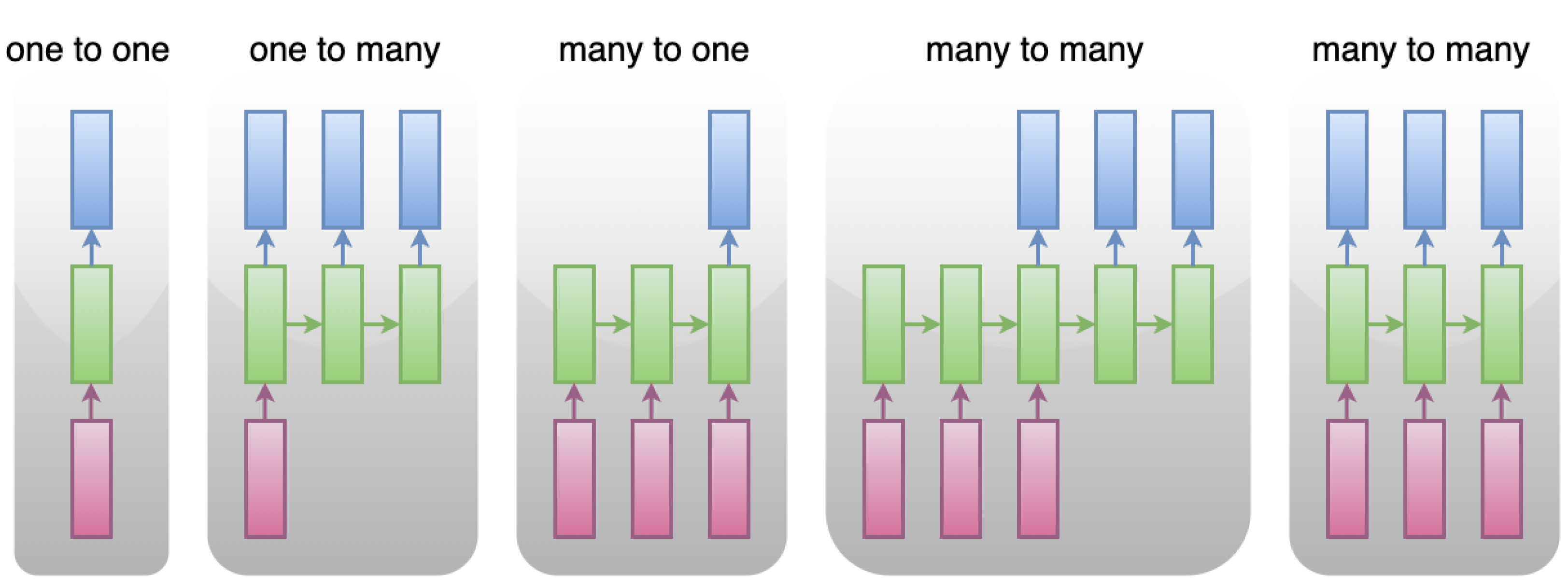
2.1. RNN for Variable Inputs/Outputs
- One to Many, applied in fields of image captioning, text generation
- Many to One, applied in fields of sentiment analysis, text classification
- Many to Many, applied in fields of machine translation, voice recognition
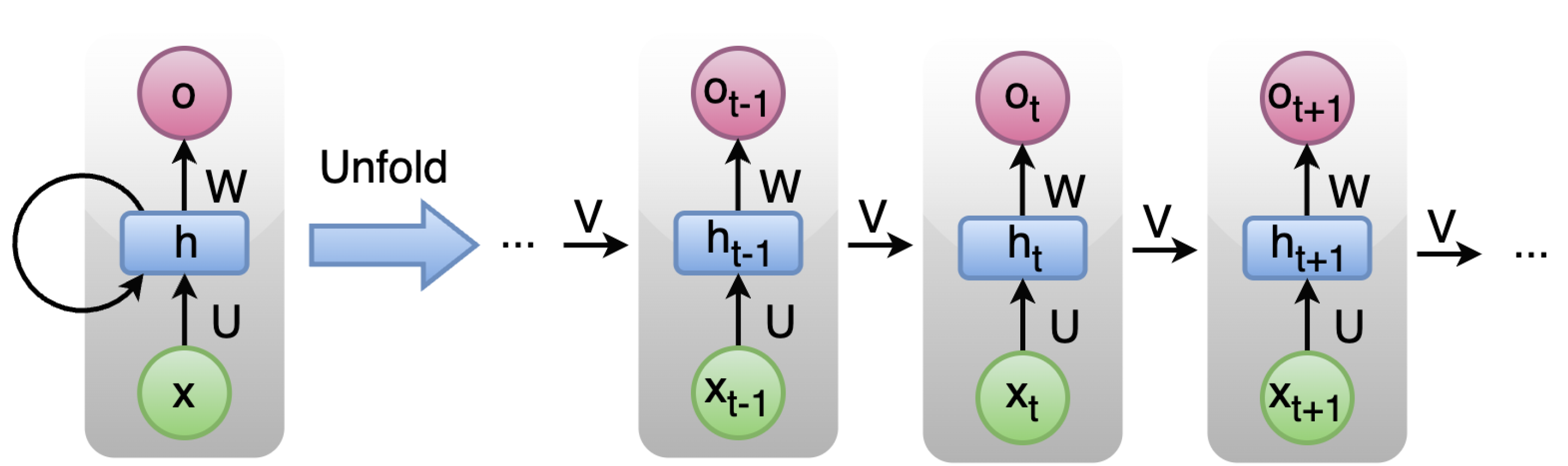
2.2. Vanilla RNN
- Inputs and outputs are of variable size
- In each stage the hidden state from the previous stage as well as the current input is utilized to compute the current hidden state that feeds the next stage. Consequently, knowledge from past data is transmitted through the hidden states to the next stages. Hence, the hidden state is a means of connecting the past with the present as well as input with output.
- The set of parameters U, V, and W as well as the activation function are common to all RNN cells.
2.3. Long Short-Term Memory
2.4. Convolutional Neural Network
2.5. Gated Recurrent Unit
3. Materials and Methods
3.1. Dataset
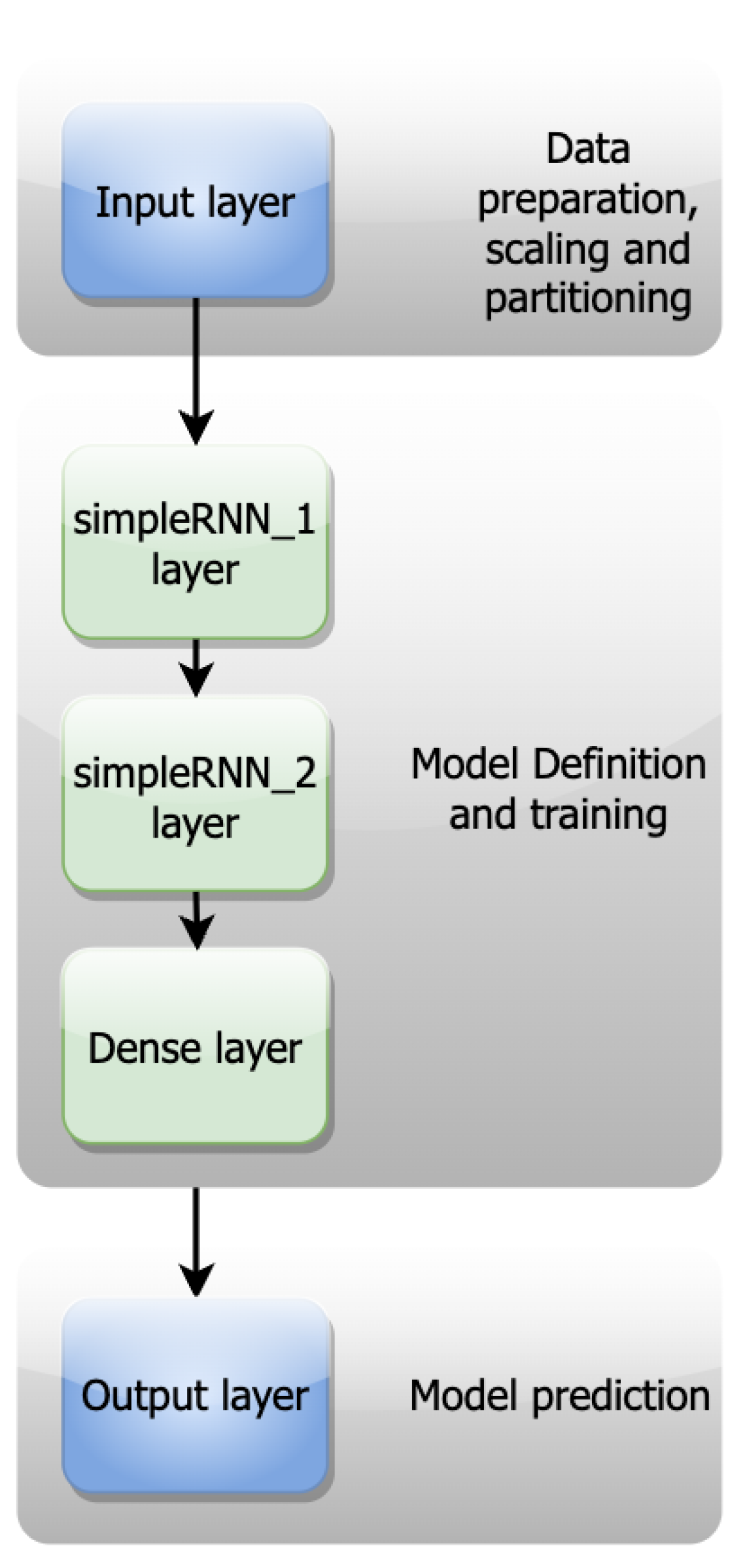
3.2. Proposed Methodology
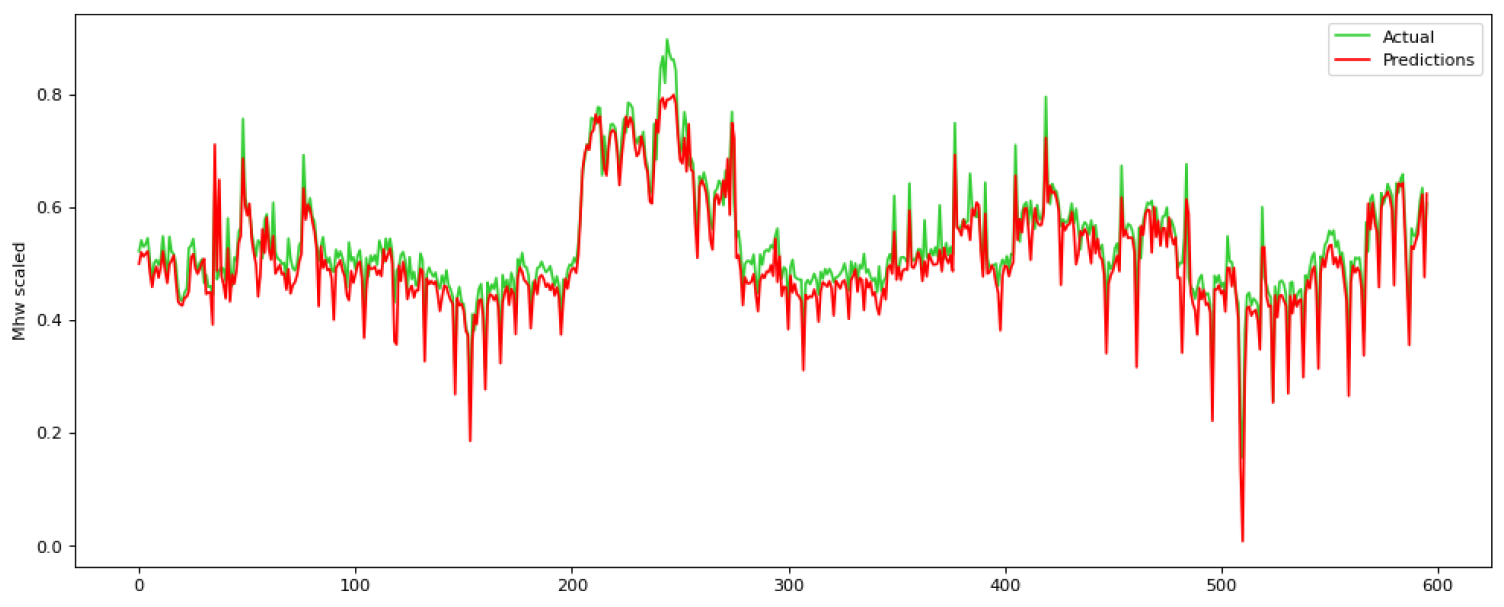
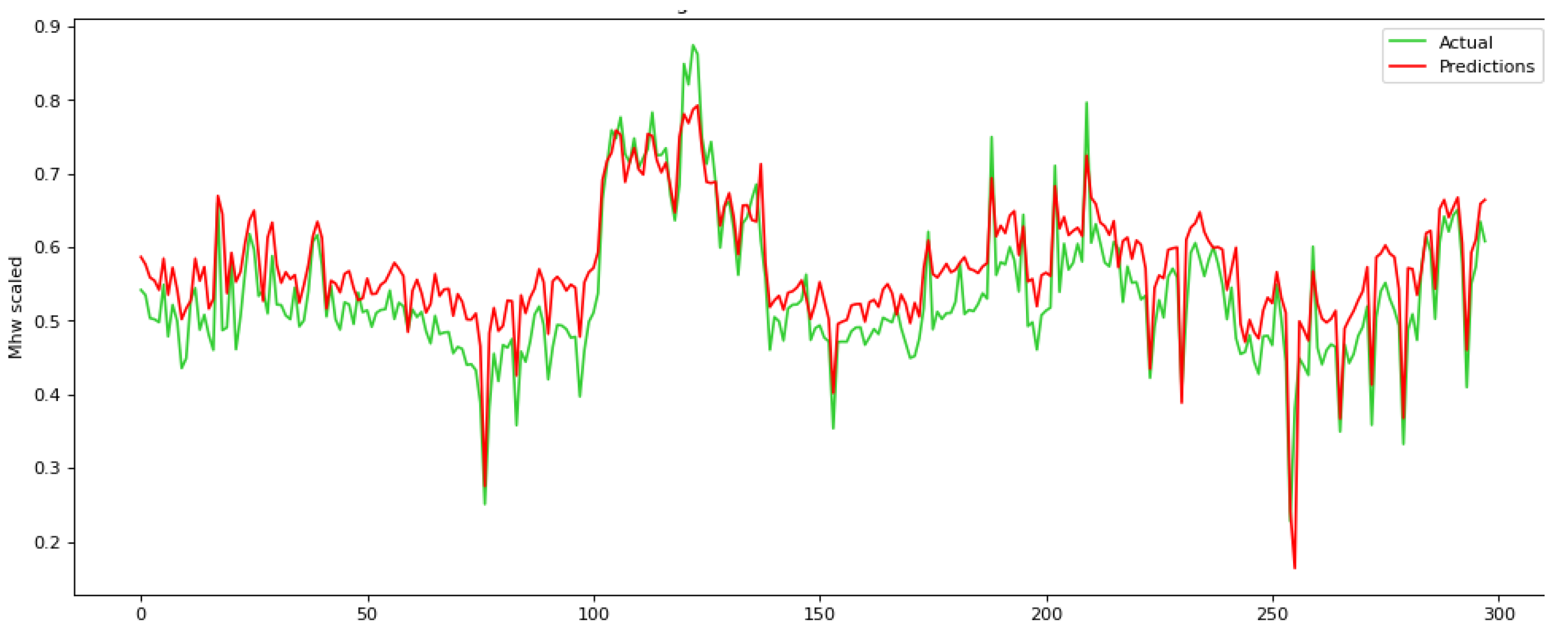
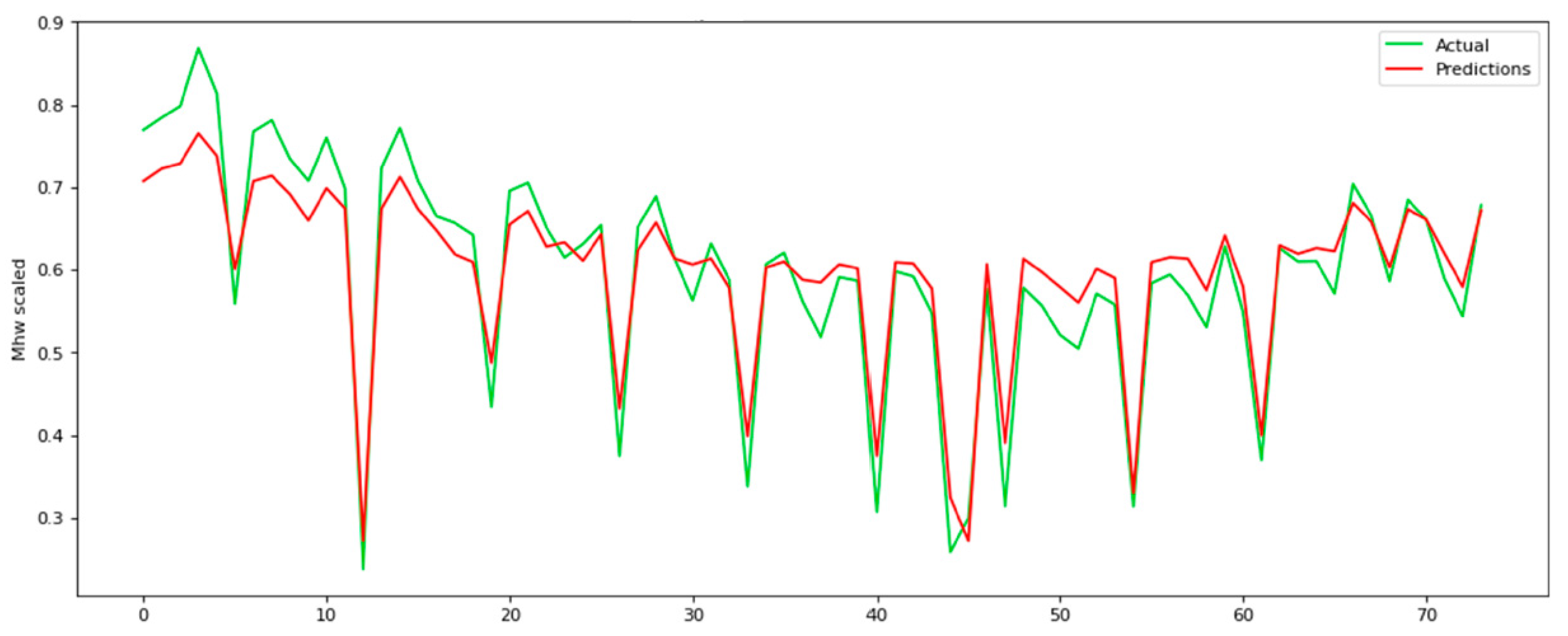
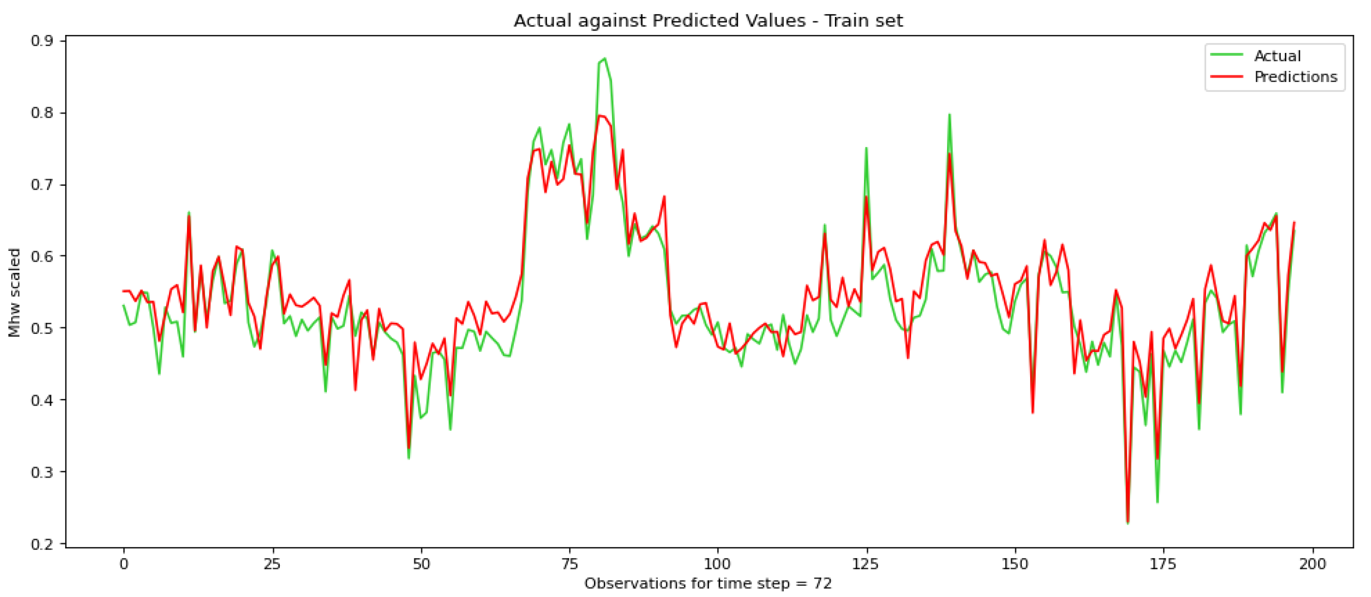
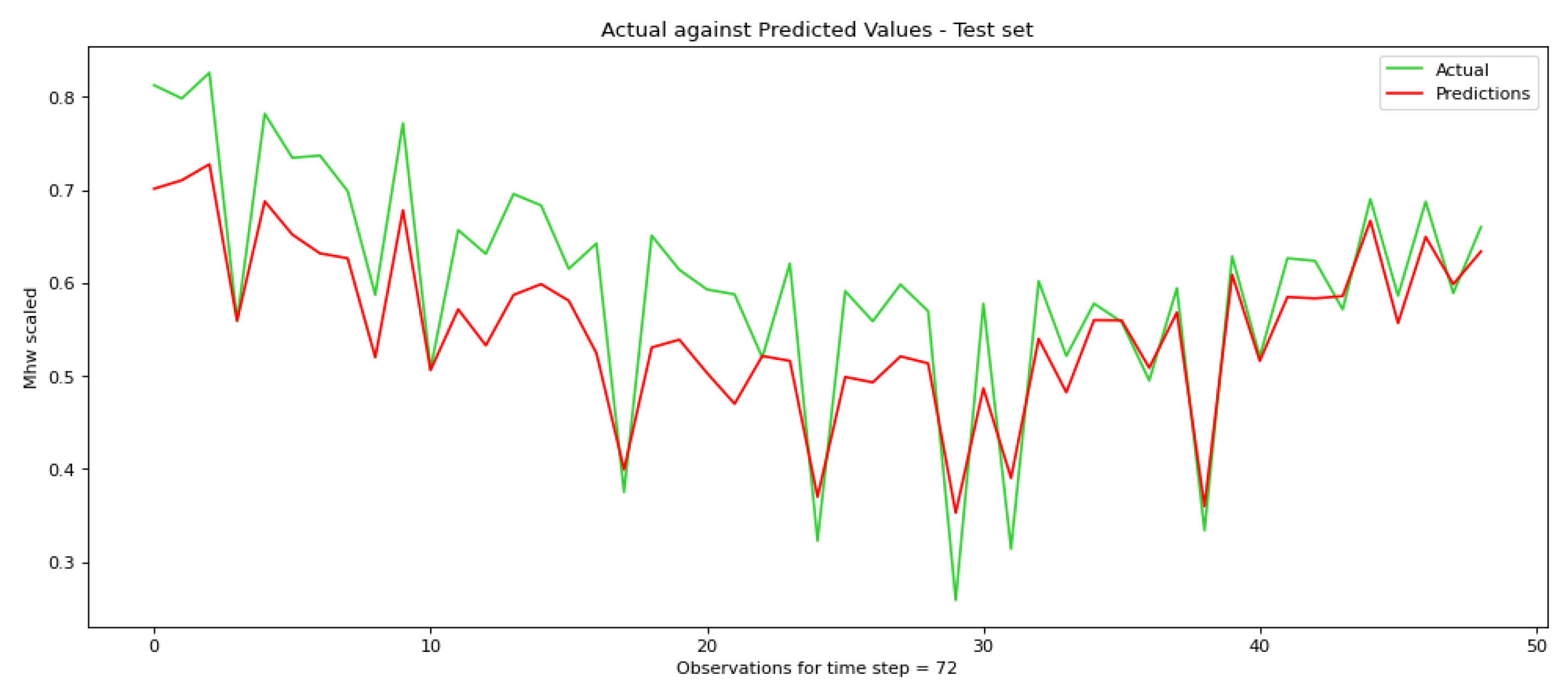
4. Results and Discussion
5. Conclusions
Author Contributions
Funding
Institutional Review Board Statement
Informed Consent Statement
Data Availability Statement
Conflicts of Interest
Abbreviations
| AGC | Automatic Generation Control |
| ANN | Artificial Neural Network |
| CNN | Convolutional Neural Network |
| DSO | Distribution System Operators |
| ELD | Economic Load Dispatch |
| GRU | Gated Recurrent Unit |
| HETS | Hellenic Electricity Transmission System |
| IPTO | Independent Power Transmission Operator |
| LD | Linear dichroism |
| LSTM | Long Short-Term Memory |
| LTF | Long-term forecasting |
| MAE | Mean Absolute Error |
| MTF | Medium-term forecasting |
| RMSE | Root Mean Square Error |
| RNN | Recurrent Neural Network |
| STF | Short-term forecasting |
| TSO | Transmission System Operator |
References
- Kang, C.; Xia, Q.; Zhang, B. Review of power system load forecasting and its development. Autom. Electr. Power Syst. 2004, 28, 1–11. [Google Scholar]
- Shi, T.; Lu, F.; Lu, J.; Pan, J.; Zhou, Y.; Wu, C.; Zheng, J. Phase Space Reconstruction Algorithm and Deep Learning-Based Very Short-Term Bus Load Forecasting. Energies 2019, 12, 4349. [Google Scholar] [CrossRef]
- Zhang, K.; Tian, X.; Hu, X.; Guo, Z.N. Partial Least Squares regression load forecasting model based on the combination of grey Verhulst and equal-dimension and new-information model. In Proceedings of the 7th International Forum on Electrical Engineering And Automation (IFEEA), Hefei, China, 25–27 September 2020; pp. 915–919. [Google Scholar] [CrossRef]
- Liu, Z.; Wang, X.; Pan, S.; Zhang, M.; Ji, Y.Z. Midterm Power Load Forecasting Model Based on Kernel Principal Compo-nent Analysis. Big Data 2019, 7, 130–138. [Google Scholar] [CrossRef] [PubMed]
- Al-Hamadi, H.; Soliman, S.A. Long-term/mid-term electric load forecasting based on short-term correlation and annual growth. Electr. Power Syst. Res. 2005, 74, 353–361. [Google Scholar] [CrossRef]
- Baek, S. Mid-term Load Pattern Forecasting with Recurrent Artificial Neural Network. IEEE Access 2019, 7, 172830–172838. [Google Scholar] [CrossRef]
- Nalcaci, G.; Ozmen, A.; Weber, G.W. Long-term load forecasting: Models based on MARS, ANN and LR methods. Cent. Eur. J. Oper. Res. 2019, 27, 1033–1049. [Google Scholar] [CrossRef]
- Adhiswara, R.; Abdullah, A.G.; Mulyadi, Y. Long-term electrical consumption forecasting using Artificial Neural Network (ANN). J. Phys. Conf. Ser. 2019, 1402, 033081. [Google Scholar] [CrossRef]
- Tsakoumis, A.C.; Vladov, S.S.; Mladenov, V.M. Electric load forecasting with multilayer perceptron and Elman neural network. In Proceedings of the 6th Seminar on Neural Network Applications in Electrical Engineering, Belgrade, Yugoslavia, 26–28 September 2002; pp. 87–90, ISBN 0-7803-7593-9. [Google Scholar] [CrossRef]
- Dondon, P.; Carvalho, J.; Gardere, R.; Lahalle, P.; Tsenov, G.; Mladenov, V. Implementation of a feed-forward Artificial Neural Network in VHDL on FPGA. In Proceedings of the 12th Symposium on Neural Network Applications in Electrical Engineering, Belgrade, Serbia, 25–27 November 2014; pp. 37–40, ISBN 978-147995888-7. [Google Scholar] [CrossRef]
- Abu-Shikhah, N.; Aloquili, F.; Linear, O.; Regression, N. Smart Grid and Renewable Energy. Smart Grid Renew. Energy 2011, 2, 126–135. [Google Scholar] [CrossRef]
- Pappas, S.; Ekonomou, L.; Moussas, V.C.; Karampelas, P.; Katsikas, S.K. Adaptive Load Forecasting Of The Hellenic Electric Grid. J. Zhejiang Univ. Sci. 2008, 2, 1724–1730. [Google Scholar] [CrossRef]
- Pappas, S.; Ekonomou, L.; Karampelas, P.; Karamousantas, D.C.; Katsikas, S.K.; Chatzarakis, G.E.; Skafidas, P.D. Electricity Demand Load Forecasting of the Hellenic Power System Using an ARMA Model. Electr. Power Syst. Res. 2010, 80, 256–264. [Google Scholar] [CrossRef]
- Ekonomou, L.; Oikonomou, S.D. Application and comparison of several artificial neural networks for forecasting the Hellenic daily electricity demand load. In Proceedings of the 7th WSEAS International Conference on Artificial Intelligence, Knowledge Engineering and Data Bases (AIKED’ 08), Cambridge, UK, 20–22 February 2008; pp. 67–71. [Google Scholar]
- Ekonomou, L.; Christodoulou, C.A.; Mladenov, V. A short-term load forecasting method using artificial neural networks and wavelet analysis. Int. J. Power Syst. 2016, 1, 64–68. [Google Scholar]
- Karampelas, P.; Pavlatos, C.; Mladenov, V.; Ekonomou, L. Design of artificial neural network models for the prediction of the Hellenic energy consumption. In Proceedings of the 10th Symposium on Neural Network Applications in Electrical Engineering, Belgrade, Serbia, 23–25 September 2010. [Google Scholar]
- Hwan, K.J.; Kim, G.W. A short-term load forecasting expert system. In Proceedings of the 5th Korea-Russia International Symposium on Science and Technology, Tomsk, Russia, 26 June–3 July 2001; Volume 1, pp. 112–116. [Google Scholar]
- Ali, M.; Adnan, M.; Tariq, M.; Poor, H.V. Load Forecasting through Estimated Parametrized Based Fuzzy Inference System in Smart Grids. IEEE Trans. Fuzzy Syst. 2021, 29, 156–165. [Google Scholar] [CrossRef]
- Bhotto, M.Z.A.; Jones, R.; Makonin, S.; Bajić, I.V. Short-Term Demand Prediction Using an Ensemble of Linearly-Constrained Estimators. IEEE Trans. Power Syst. 2021, 36, 3163–3175. [Google Scholar] [CrossRef]
- Jiang, H.; Zhang, Y.; Muljadi, E.; Zhang, J.J.; Gao, D.W. A Short-Term and High-Resolution Distribution System Load Forecasting Using Support Vector Regression with Hybrid Parameters Optimization. IEEE Trans. Smart Grid 2018, 9, 3341–3350. [Google Scholar] [CrossRef]
- Li, G.; Li, Y.; Roozitalab, F. Midterm Load Forecasting: A Multistep Approach Based on Phase Space Reconstruction and Sup-port Vector Machine. IEEE Syst. J. 2020, 14, 4967–4977. [Google Scholar] [CrossRef]
- Zafeiropoulou, M.; Sijakovic, I.; Terzic, N.; Fotis, G.; Maris, T.I.; Vita, V.; Zoulias, E.; Ristic, V.; Ekonomou, L. Forecasting Transmission and Distribution System Flexibility Needs for Severe Weather Condition Resilience and Outage Management. Appl. Sci. 2022, 12, 7334. [Google Scholar] [CrossRef]
- Fotis, G.; Vita, V.; Maris, I.T. Risks in the European Transmission System and a Novel Restoration Strategy for a Power System after a Major Blackout. Appl. Sci. 2023, 23, 83. [Google Scholar] [CrossRef]
- Sambhi, S.; Kumar, H.; Fotis, G.; Vita, V.; Ekonomou, L. Techno-Economic Optimization of an Off-Grid Hybrid Power Generation for SRM IST Delhi-NCR Campus. Energies 2022, 15, 7880. [Google Scholar] [CrossRef]
- Sambhi, S.; Bhadoria, H.; Kumar, V.; Chaurasia, P.; Chaurasia, G.S.; Fotis, G.; Vita, G.; Ekonomou, V.; Pavlatos, C. Economic Feasibility of a Renewable Integrated Hybrid Power Generation System for a Rural Village of Ladakh. Energies 2022, 15, 9126. [Google Scholar] [CrossRef]
- Khuntia, S.; Rueda, J.; Meijden, M. Forecasting the load of electrical power systems in mid- and long-term horizons: A review. IET Gener. Transm. Distrib. 2016, 10, 3971–3977. [Google Scholar] [CrossRef]
- Directive (EU) 2019/944 of the European Parliament and of the Council of 5 June 2019 on Common Rules for the Internal Market for Electricity and Amending Directive 2012/27/EU. Available online: https://eur-lex.europa.eu/legal-content/EN/TXT/?qid=1570790363600&uri=CELEX:32019L0944 (accessed on 29 December 2022).
- IRENA. Innovation Landscape Brief: Market Integration of Distributed Energy Resources; International Renewable Energy Agency: Abu Dhabi, United Arab Emirates, 2019. [Google Scholar]
- Commission, M.; Company, D. Integrating Renewables into Lower Michigan Electric Grid. Available online: https://www.brattle.com/wp-content/uploads/2021/05/15955_integrating_renewables_into_lower_michigans_electricity_grid.pdf (accessed on 29 December 2022).
- Wang, F.C.; Hsiao, Y.S.; Yang, Y.Z. The Optimization of Hybrid Power Systems with Renewable Energy and Hydrogen Gen-eration. Energies 1948, 11, 1948. [Google Scholar] [CrossRef]
- Wang, F.; Lin, K.-M. Impacts of Load Profiles on the Optimization of Power Management of a Green Building Employing Fuel Cells. Energies 2019, 12, 57. [Google Scholar] [CrossRef]
- Sun, W.; Zhang, C. A Hybrid BA-ELM Model Based on Factor Analysis and Similar-Day Approach for Short-Term Load Forecasting. Energies 2018, 11, 1282. [Google Scholar] [CrossRef]
- Goller, C.; Kuchler, A. Learning task-dependent distributed representations by backpropagation through structure. In Proceedings of the International Conference on Neural Networks (ICNN’96), Washington, DC, USA, 3–6 June 1996; Volume 1, pp. 347–352. [Google Scholar]
- Sherstinsky, A. Fundamentals of recurrent neural network (RNN) and long short-term memory (LSTM) network. Phys. D Nonlinear Phenom. 2020, 404, 132306. [Google Scholar] [CrossRef]
- Hochreiter, S.; Schmidhuber, J. Long Short-Term Memory. Neural Comput. 1997, 9, 1735–1780. [Google Scholar] [CrossRef]
- Lecun, Y.; Bottou, L.; Bengio, Y.; Haffner, P. Gradient-based learning applied to document recognition. Proc. IEEE 1998, 86, 2278–2324. [Google Scholar] [CrossRef]
- Abdel-Basset, M.; Moustafa, N.; Hawash, H. Dive Into Recurrent Neural Networks. In Deep Learning Approaches for Security Threats in IoT Environments; IEEE: Piscataway, NJ, USA, 2023; pp. 209–229. [Google Scholar]
- Cho, K.; Van Merriënboer, B.; Bahdanau, D.; Bengio, Y. On the properties of neural machine translation: Encoder-decoder approaches. arXiv 2014, arXiv:1409.1259. [Google Scholar]
- Available online: https://www.data.gov.gr/datasets/admie_realtimescadasystemload/ (accessed on 29 December 2022).


| Time Horizon | Area of Application |
|---|---|
| 12 months–20 months | Planning of the Power System |
| 1 week–12 months | Scheduling the maintenance of the power system elements |
| 1 min–1 week | Commitment analysis of the power units |
| Automatic Generation Control (AGC) | |
| Economic load dispatch (ELD) | |
| ms–s | Power system dynamic analysis |
| ns–ms | Power system transient analysis |
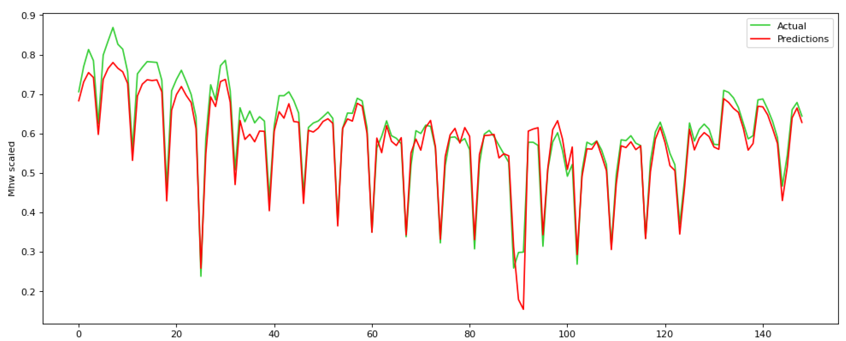
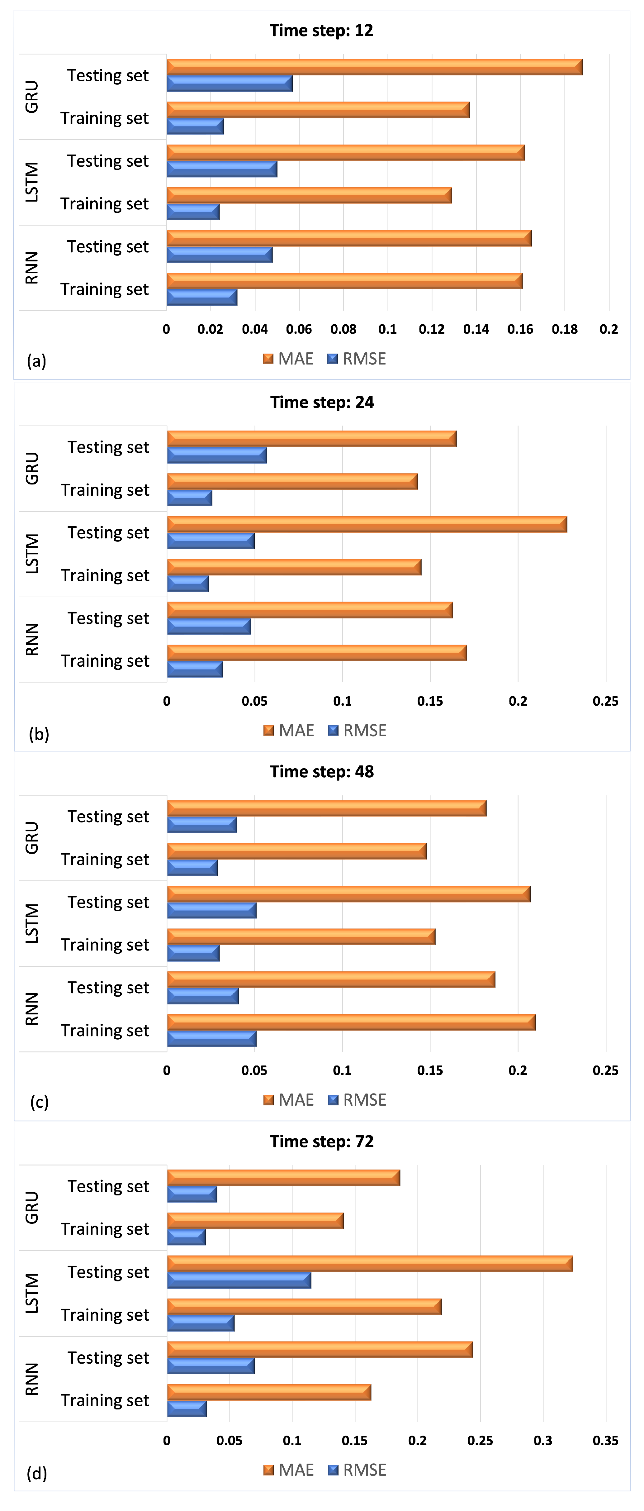
| Time Step | 12 | 24 | 48 | 72 | |||||
|---|---|---|---|---|---|---|---|---|---|
| RMSE | MAE | RMSE | MAE | RMSE | MAE | RMSE | MAE | ||
| RNN | Training set | 0.032 | 0.161 | 0.038 | 0.171 | 0.051 | 0.210 | 0.032 | 0.163 |
| Testing set | 0.048 | 0.165 | 0.033 | 0.163 | 0.041 | 0.187 | 0.070 | 0.244 | |
| LSTM | Training set | 0.024 | 0.129 | 0.030 | 0.145 | 0.030 | 0.153 | 0.054 | 0.219 |
| Testing set | 0.050 | 0.162 | 0.055 | 0.228 | 0.051 | 0.207 | 0.115 | 0.324 | |
| GRU | Training set | 0.026 | 0.137 | 0.032 | 0.143 | 0.029 | 0.148 | 0.031 | 0.141 |
| Testing set | 0.057 | 0.188 | 0.033 | 0.165 | 0.040 | 0.182 | 0.040 | 0.186 | |
Disclaimer/Publisher’s Note: The statements, opinions and data contained in all publications are solely those of the individual author(s) and contributor(s) and not of MDPI and/or the editor(s). MDPI and/or the editor(s) disclaim responsibility for any injury to people or property resulting from any ideas, methods, instructions or products referred to in the content. |
© 2023 by the authors. Licensee MDPI, Basel, Switzerland. This article is an open access article distributed under the terms and conditions of the Creative Commons Attribution (CC BY) license (https://creativecommons.org/licenses/by/4.0/).
Share and Cite
Pavlatos, C.; Makris, E.; Fotis, G.; Vita, V.; Mladenov, V. Utilization of Artificial Neural Networks for Precise Electrical Load Prediction. Technologies 2023, 11, 70. https://doi.org/10.3390/technologies11030070
Pavlatos C, Makris E, Fotis G, Vita V, Mladenov V. Utilization of Artificial Neural Networks for Precise Electrical Load Prediction. Technologies. 2023; 11(3):70. https://doi.org/10.3390/technologies11030070
Chicago/Turabian StylePavlatos, Christos, Evangelos Makris, Georgios Fotis, Vasiliki Vita, and Valeri Mladenov. 2023. "Utilization of Artificial Neural Networks for Precise Electrical Load Prediction" Technologies 11, no. 3: 70. https://doi.org/10.3390/technologies11030070