
HADD: High-Accuracy Detection of Depressed Mood

Abstract
:1. Introduction
- HADD is new in that it supports multimodal analysis of mobile data consisting of subjective EMA data and objective sensor data to enhance the accuracy of the detection of depressed mood. Despite the potential synergy that can be created by analyzing multimodal data, research on detecting depressed mood by analyzing EMA and passive sensing data is in an early stage, and related work is relatively scarce [26,27,28,29,30].
- To support high accuracy in depressed mood detection even when the given/available dataset is small and imbalanced, HADD enhances state-of-the-art ML models as follows: (1) HADD supports effective data augmentation equipped with a self-validity check; (2) it selects key features from a comprehensive set of multimodal mobile/wearable data to support high-accuracy detection of depressed mood with minimal model complexity; (3) HADD supports a new two-stage detection method that detects depressed mood in two stages in order to detect anomalies (depressed mood) with a high accuracy even when the available dataset is small and imbalanced. In the first stage, a state-of-the-art supervised ML model is used to detect/classify depressed mood in users on a daily basis. In the second stage, we analyze the statistical distribution of the daily detection results collected for an extended period of time, such as a month, to detect outliers—users with a depressed mood. By doing this, HADD aims to avoid misclassifying transient mood changes in healthy users as indicating a depressed mood and to further enhance the accuracy of depressed mood detection. Notably, our proposed techniques are not tied to a specific ML model, but are generally applicable to enhance the accuracy of ML models for depressed mood detection.
- HADD is a new general machine learning framework for depressed mood detection and is not tied to a specific machine learning model, unlike the examples in the related work discussed in Section 2. It can support a wide variety of machine learning models and, therefore, enables a mental healthcare provider (MHP) to choose a model that is most appropriate for their job. In this paper, we use 12 machine learning models and compare their performance by evaluating each model in HADD, one by one. An MHP can choose any of the models based on, for example, the detection accuracy or explainability. Furthermore, HADD is extensible: An MHP or a data scientist can easily add new models if necessary.
- In this paper, we thoroughly evaluate the performance of HADD by using the StudentLife dataset [12]. It is a relatively small dataset that consists of many subjective and objective features that were collected using smartphones. HADD enhances the accuracy of depressed mood detection by 17% on average in comparison with the accuracy of 12 state-of-the-art ML models that all used subjective/objective features without feature selection and did not exploit the data augmentation or two-stage outlier detection supported by HADD.
2. Related Work
2.1. EMA/Questionnaires
2.2. Passive Sensing
2.3. EMA and Passive Sensing
3. HADD
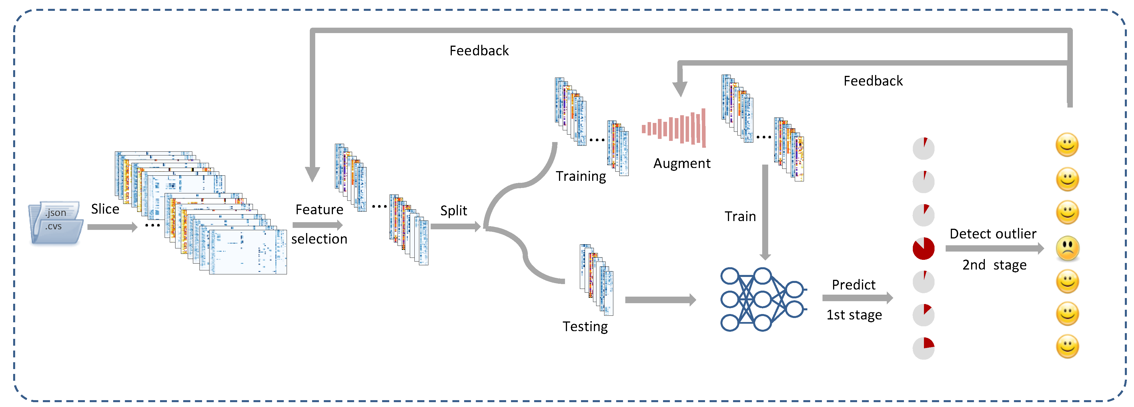
3.1. An Overview of the Method
- Data preparation: In this paper, we divided the input data into 24 h slices to enable daily detection of depressed mood, as illustrated in Figure 1. In this paper, we considered that a user had a depressed mood if their PHQ-9 score was at least 10 (moderately depressed [10]); however, our approach can be used with different depression screening instruments, such as BDI-II. A more detailed discussion of the data preprocessing is given in Section 4.
- Feature selection: As shown in Figure 1, we selected a subset of the features that were closely correlated with depression to support high accuracy with minimal model complexity and computational overhead.
- Data augmentation: To support high accuracy even when the available dataset is small, we augmented the training set, if necessary, to enhance the accuracy by mitigating the imbalance between the samples in depressed and non-depressed moods, as depicted in Figure 1.
- Two-stage detection of depressed mood: To further enhance the prediction performance, we also propose a new method for the two-stage detection of depressed mood. In the first stage, HADD runs a trained ML model against each participant’s daily data to estimate their depressed mood over an extended period of time, such as several weeks or months. In the second phase, HADD analyzes the statistical distribution to detect outliers, i.e., users with depressed mood, as illustrated in Figure 1.
3.2. Feature Selection
3.3. Augmenting Training Data
- 1.
- Initialize the augmentation factor .
- 2.
- Perform data augmentation using .
- 3.
- Compute the statistical distribution and check the validity.
- 4.
- If the validity check is successful, save the augmented dataset and increment by 1. Go to Step 2.
- 5.
- Otherwise, abort the augmentation and revert to the dataset generated in the previous iteration. Revert to the original dataset if the validity check fails when . Stop data augmentation and exit.
3.4. Two-Stage Detection of Depressed Mood
3.4.1. Stage 1
- Logistic Regression (LR) is one of the most popular classification algorithms. It uses the sigmoid function as the cost function:where is the set of the features and represents the model parameters. In the training phase, it minimizes the cost function and learns by using the gradient descent method. It then uses the trained model to classify new data unseen during the training.
- A Support Vector Machine (SVM) finds a hyperplane that has the maximum margin against the support vectors in order to divide training samples into the classes. The SVM supports effective classification if data are linearly separable. Otherwise, its performance may not be significantly different from that provided by LR.
- k-Nearest Neighbors (kNN) computes the distance from a new test data to the stored training data. The k-nearest data then determine the class of the new data via voting.
- A Decision Tree (DT) mimics the human decision process by constructing a tree in which each non-leaf node splits based on a feature. Thus, it is human-interpretable if it is short. A deeper tree tends to be harder to interpret and subject to overfitting.
- The Gradient-Boosting Decision Tree (GBDT), Ada Boost (AB), and Random Forest (RF) trade the interpretability of DT for performance by leveraging ensemble learning. In the GBDT and AB, each DT model learns from the error of the previous model. In contrast, the RF applies the bagging method. The DT models in an RF use randomly selected features and learn in parallel. The trained models in the RF classify new data via the majority vote.
- Gaussian Naive Bayes (GNB) is a variant of Naive Bayes that uses the Bayes theorem under the naive assumption that features are independent. GNB assumes that the density of each class is normally distributed.
- Linear Discriminant Analysis (LDA) is simple yet powerful. It uses a linear discriminant function based on the Bayesian and maximum likelihood rules to determine the region (class) to which data belong under the assumption that all classes share the same covariance matrix.
- Quadratic Discriminant Analysis (QDA) uses a quadratic discriminant function. In addition, it does not make the assumption of a shared covariance matrix across classes, unlike LDA. In general, it is more flexible than LDA, but is more susceptible to overfitting than LDA is. For more details on LDA and QDA, interested readers are referred to [58].
- A Deep Neural Network (DNN) is effective for ML due to its capability of nonlinear approximation. In this paper, we designed a DNN that consisted of four fully connected layers with 64, 32, 16, and 2 neurons to classify participants as depressed or non-depressed.
- A Convolutional Neural Network (CNN) is powerful in many ML tasks, e.g., computer vision. In this paper, we designed a CNN that consisted of a convolution layer and three fully connected layers with 64, 32, 16, and 2 neurons, respectively. For convolution, the kernel size was 2 and stride was 1. Following convolution, the CNN performed max pooling.
3.4.2. Stage 2
- 1.
- HADD builds the vector , where the random variable is defined in Equation 3 and collected for each user in Stage 1.
- 2.
- It computes the mean, , and standard deviation, , of the vector .
- 3.
- Finally, HADD classifies the client i as class 1 (being in a depressed mood) if the following condition holds:where is looked up in the t-table using the confidence level and the degrees of freedom [60].
4. Evaluation
4.1. Data Preparation
4.1.1. Dataset
4.1.2. Data Preprocessing
4.1.3. Data Augmentation
4.1.4. Selecting Objective and Subjective Features

| Item | Feature | r | p-Value |
|---|---|---|---|
| 1 | Dark_duration | 0.117010485 | 7.33954 |
| 2 | Conversation_duration | −0.10050095 | 4.12932 |
| 3 | PAM_picture_idx | 0.086854646 | 3.82635 |
| 4 | Audio_inference | −0.082883614 | 1.26971 |
| 5 | Mood_happyornot | 0.081726937 | 1.78281 |
| 6 | Sleep_social | 0.080808105 | 2.32707 |
| 7 | Mood_sad | 0.075941272 | 9.10363 |
| 8 | Phonecharge_duration | 0.070690366 | 3.63055 |
| 9 | Phonelock_duration | 0.063472895 | 0.000209513 |
| 10 | Class_experience | 0.055680536 | 0.001148481 |
| 11 | Sleep_rate | 0.050727791 | 0.003058695 |
| 12 | Administration response_apathetic | 0.049628777 | 0.003761137 |
| 13 | Activity_inference | −0.047794521 | 0.005265698 |
| 14 | Boston Bombing_boston | 0.047554704 | 0.005498195 |
| 15 | Dimensions protestors_appreciative | 0.045303212 | 0.008176002 |
| 16 | Dimensions protestors_proud | 0.044667622 | 0.009118687 |
| 17 | Mood_tomorrow | 0.04460978 | 0.009209115 |
| 18 | Stress_level | 0.044346094 | 0.00963156 |
| 19 | Exercise_exercise | −0.04327199 | 0.01153625 |
| 20 | Dimensions protestors_empathic | 0.042928071 | 0.01221311 |
| 21 | Behavior_sympathetic | 0.042189111 | 0.013787576 |
| 22 | Dining Halls_dinner | -0.03940632 | 0.021438194 |
| 23 | Class_hours | 0.036251256 | 0.034354408 |
| 24 | Administration response_appreciative | 0.036075483 | 0.035237284 |
| 25 | Lab_duration | 0.0310954 | 0.06955524 |
| 26 | Exercise_schedule | −0.029959267 | 0.080384652 |
| ... | ... | ... | ... |
| 76 | Dartmouth now_saddened | −0.001650002 | 0.92330252 |
| 77 | Behavior_critical | −0.00147211 | 0.931549995 |
| 78 | Dartmouth now_frustrated | 3.92106 | 0.99817455 |
- 1.
- Dark duration indicates the length of the time period for which the screen remains dark for more than one hour.
- 2.
- Audio inference continuously detected audio signals using the microphone (0: silence, 1: voice, 2: noise, 3: unknown).
- 3.
- Phone charge duration records the time spent charging the smartphone.
- 4.
- Activity was continuously analyzed using the accelerometer (0: stationary, 1: walking, 2: running, 3: unknown).
- 1.
- PAM_pictur_idx: A participant selected a picture that best represented their mood from a grid of 16 pictures provided randomly from a library of 48 photos designed for a photographic affect meter (PAM) [61].
- 2.
- mood_happy_or_not question: “Do you feel at all happy right now?” (1: yes, 2: no).
- 3.
- sleep_social question: “How often did you have trouble staying awake yesterday while in class, eating meals, or engaging in social activity?” (1: none, 2: once, 3: twice, 4: three or more times).
- 4.
- mood_sad question: “How sad do you feel?” (1: a little bit, 2: somewhat, 3: very much, 4: extremely).
- 5.
- sleep_rate question: “How would rate your overall sleep last night?” (1: very good, 2: fairly good, 3: fairly bad, 4: very bad).
- 6.
- stress_level question: “Stress level?” (1: a little stressed, 2: definitely stressed, 3: stressed out, 4: feeling good, 5: feeling great).
4.2. Tuning the Model Parameters
- LR: We set L-BFGS (Limited-Memory Broyden–Fletcher–Goldfarb–Shanno) algorithm [65] as the optimizer to tune the logistic regression parameters in a gradient-descent manner with an L2 norm regularization penalty, which is known as ridge regression, to reduce overfitting.
- SVM: We used the radial basis function (RBF) kernel to support the nonlinear classification. To avoid possible overfitting, we set the generalization penalty parameter to C = 1.0 and the kernel coefficient to , where is the number of features and is the variance of the training data.
- kNN: In kNN, the number of neighbors k affects the performance. We used the Euclidean distance to measure the error. We set to minimize the error by trial and error.
- DT: We used the Gini impurity as the classification criterion for splitting the nodes to build the decision tree by using the training data.
- AB, GBDT, and RF: These ensemble models are designed to be more robust to noise than a simple decision tree by aggregating multiple weak learners. We used a decision tree classifier as the weak learner/base estimator for all three of these ensemble algorithms. We set the numbers of trees to 50, 100, and 10 for AB, GBDT, and RF, respectively. A more detailed description of the process for tuning AB, GBDT, and RF follows.
- –
- For AB, we set the learning rate to 1.0, and used the boosting algorithm of SAMME.R. AB built the model by adding up the weights of each tree, which were learned and updated via iterations.
- –
- For GBDT, we set the learning rate to 0.1, the maximum depth of a tree to 3, and the minimum sample leaf to 1. GBDT calculated the residual from the previous tree and aggregated all of them as the whole model.
- –
- To configure RF, we set the square root of the total number of the features as the maximum number of features for each individual tree, and we set the minimum sample leaf to 1. RF randomly selected subsets of features from the training set to build the decision trees and make the final decision with the majority vote.
- GNB: The GNB model applied the Bayes theorem in order to calculate the conditional probability of each label under every selected feature of the training data.
- LDA and QDA: LDA and QDA both used the Bayes rule to fit the class-conditional probability densities to the training data and build the decision boundary. LDA assumed that there was a common covariance of both classes, while QDA considered a separate covariance for each class.
- DNN and CNN: To train both the DNN and CNN, we randomly picked one-third of the training set as a validation set and performed cross-validation to tune the model parameters carefully, thus avoiding overfitting. We used the stochastic gradient descent algorithm to tune the parameters by using the mean squared error (MSE) as the loss function. We also used the Adam optimizer [66]. Specifically, the batch size was 32. We had a total of 200 epochs with a learning rate of 0.001.
4.3. Evaluation Results
4.3.1. Effectiveness of the Multimodal Approach in Detecting Depressed Mood
- 1.
- B1 (all features): This baseline simply uses all 78 features in the StudentLife dataset to predict depression.
- 2.
- 3.
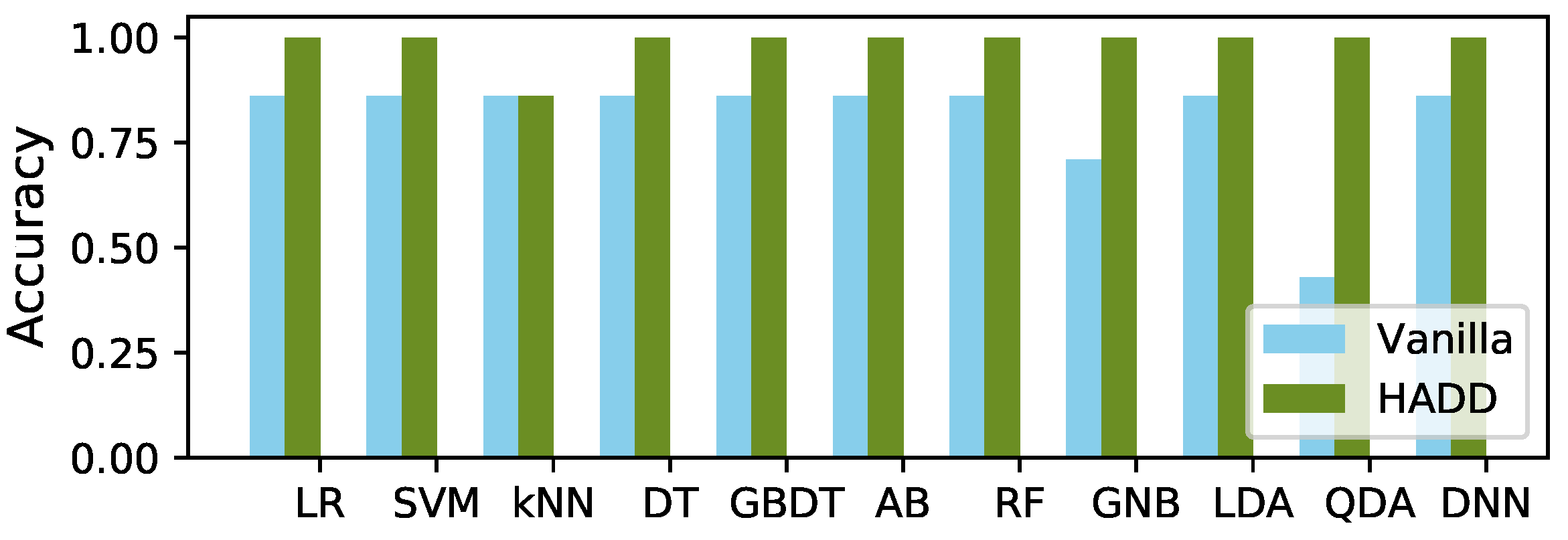
4.3.2. Overall Accuracy Improvement by HADD
5. Conclusions and Future Work
Author Contributions
Funding
Data Availability Statement
Conflicts of Interest
References
- World Health Organization. Depression. Available online: https://www.who.int/news-room/fact-sheets/detail/depression (accessed on 27 September 2022).
- National Alliance on Mental Health. Mental Health By the Numbers. Available online: https://www.nami.org/mhstats (accessed on 27 September 2022).
- American Psychiatric Association Foundation. Quantifying the Cost of Depression. Available online: https://www.workplacementalhealth.org/Mental-Health-Topics/Depression/Quantifying-the-Cost-of-Depression (accessed on 27 September 2022).
- Asare, K.O.; Visuri, A.; Ferriera, D.S. Towards early detection of depression through smartphone sensing. In Proceedings of the UbiComp/ISWC 2019-Adjunct Proceedings of the 2019 ACM International Joint Conference on Pervasive and Ubiquitous Computing and Proceedings of the 2019 ACM International Symposium on Wearable Computers, London, UK, 9–13 September 2019. [Google Scholar]
- Moshe, I.; Terhorst, Y.; Asare, K.O.; Sander, L.B.; Ferreira, D.; Baumeister, H.; Mohr, D.C.; Pulkki-Råback, L. Predicting Symptoms of Depression and Anxiety Using Smartphone and Wearable Data. Front. Psychiatry 2021, 12, 625247. [Google Scholar] [CrossRef] [PubMed]
- National Network of Depression Centers. Get the Facts. Available online: https://nndc.org/facts/ (accessed on 27 September 2022).
- Marshall, J.M.; Dunstan, D.A.; Bartik, W. The Digital Psychiatrist: In Search of Evidence-Based Apps for Anxiety and Depression. Front. Psychiatry 2019, 10, 831. [Google Scholar] [CrossRef] [PubMed] [Green Version]
- Bardram, J.E.; Matic, A. A Decade of Ubiquitous Computing Research in Mental Health. IEEE Pervasive Comput. 2020, 19, 62–72. [Google Scholar] [CrossRef]
- Vahratian, A.; Blumberg, S.J.; Terlizzi, E.P.; Schiller, J.S. Symptoms of Anxiety or Depressive Disorder and Use of Mental Health Care among Adults during the COVID-19 Pandemic—United States, August 2020–February 2021. MMWR Morb. Mortal. Wkly. Rep. 2021, 70, 490–494. [Google Scholar] [CrossRef] [PubMed]
- Kroenke, K.; Spitzer, R.L.; Williams, J.B. The PHQ-9: Validity of a brief depression severity measure. J. Gen. Intern. Med. 2001, 16, 606–613. [Google Scholar] [CrossRef] [PubMed]
- Beck, A.T.; Steer, R.A.; Brown, G.K. Beck Depression Inventory-II; Psychological Corporation: San Antonio, TX, USA, 1996. [Google Scholar]
- Wang, R.; Chen, F.; Chen, Z.; Li, T.; Harari, G.; Tignor, S.; Zhou, X.; Ben-Zeev, D.; Campbell, A.T. StudentLife: Assessing mental health, academic performance and behavioral trends of college students using smartphones. In Proceedings of the 2014 ACM International Joint Conference on Pervasive and Ubiquitous Computing, Seattle, WA, USA, 13–17 September 2014; pp. 3–14. [Google Scholar]
- O’Brien, J.T.; Gallagher, P.; Stow, D.; Hammerla, N.; Ploetz, T.; Firbank, M.; Ladha, C.; Ladha, K.; Jackson, D.; McNaney, R.; et al. A study of wrist-worn activity measurement as a potential real-world biomarker for late-life depression. Psychol. Med. 2017, 47, 93–102. [Google Scholar] [CrossRef] [PubMed] [Green Version]
- da Estrela, C.; McGrath, J.; Booij, L.; Gouin, J.P. Heart rate variability, sleep quality, and depression in the context of chronic stress. Ann. Behav. Med. 2021, 55, 155–164. [Google Scholar] [CrossRef] [PubMed]
- Shatte, A.B.; Hutchinson, D.M.; Teague, S.J. Machine learning in mental health: A scoping review of methods and applications. Psychol. Med. 2019, 49, 1426–1448. [Google Scholar] [CrossRef] [Green Version]
- Thieme, A.; Belgrave, D.; Doherty, G. Machine learning in mental health: A systematic review of the HCI literature to support the development of effective and implementable ML systems. ACM Trans. Comput. Hum. Interact. (TOCHI) 2020, 27, 1–53. [Google Scholar] [CrossRef]
- Chikersal, P.; Doryab, A.; Tumminia, M.J.; Villalba, D.K.; Dutcher, J.M.; Liu, X.; Cohen, S.; Creswell, K.G.; Mankoff, J.; Creswell, J.D.; et al. Detecting Depression and Predicting its Onset Using Longitudinal Symptoms Captured by Passive Sensing: A Machine Learning Approach With Robust Feature Selection. ACM Trans. Comput. Hum. Interactation 2021, 28, 1–41. [Google Scholar] [CrossRef]
- Jacobson, N.C.; Chung, Y.J. Passive sensing of prediction of moment-to-moment depressed mood among undergraduates with clinical levels of depression sample using smartphones. Sensors 2020, 20, 3572. [Google Scholar] [CrossRef]
- Cai, H.; Han, J.; Chen, Y.; Sha, X.; Wang, Z.; Hu, B.; Yang, J.; Feng, L.; Ding, Z.; Chen, Y.; et al. A pervasive approach to EEG-based depression detection. Complexity 2018, 2018, 5238028. [Google Scholar] [CrossRef] [Green Version]
- Booij, S.H.; Bos, E.H.; Bouwmans, M.E.; van Faassen, M.; Kema, I.P.; Oldehinkel, A.J.; de Jonge, P. Cortisol and α-amylase secretion patterns between and within depressed and non-depressed individuals. PLoS ONE 2015, 10, e0131002. [Google Scholar] [CrossRef] [PubMed] [Green Version]
- Sadeque, F.; Xu, D.; Bethard, S. Measuring the latency of depression detection in social media. In Proceedings of the Eleventh ACM International Conference on Web Search and Data Mining, Los Angeles, CA, USA, 5–9 February 2018; pp. 495–503. [Google Scholar]
- Xu, X.; Chikersal, P.; Dutcher, J.M.; Sefidgar, Y.S.; Seo, W.; Tumminia, M.J.; Villalba, D.K.; Cohen, S.; Creswell, K.G.; Creswell, J.D.; et al. Leveraging Collaborative-Filtering for Personalized Behavior Modeling: A Case Study of Depression Detection among College Students. Proc. ACM Interact. Mob. Wearable Ubiquitous Technol. 2021, 5, 1–27. [Google Scholar] [CrossRef]
- Nasir, M.; Jati, A.; Shivakumar, P.G.; Nallan Chakravarthula, S.; Georgiou, P. Multimodal and multiresolution depression detection from speech and facial landmark features. In Proceedings of the 6th International Workshop on Audio/Visual Emotion Challenge, Amsterdam, The Netherlands, 16 October 2016; pp. 43–50. [Google Scholar]
- Shen, J.; Zhao, S.; Yao, Y.; Wang, Y.; Feng, L. A novel depression detection method based on pervasive EEG and EEG splitting criterion. In Proceedings of the 2017 IEEE International Conference on Bioinformatics and Biomedicine (BIBM), Kansas City, MO, USA, 13–16 November 2017; pp. 1879–1886. [Google Scholar]
- Estrin, D. A survey on image data augmentation for deep learning. Commun. ACM 2014, 57, 32–34. [Google Scholar] [CrossRef]
- Minaeva, O.; Riese, H.; Lamers, F.; Antypa, N.; Wichers, M.; Booij, S.H. Screening for depression in daily life: Development and external validation of a prediction model based on actigraphy and experience sampling method. J. Med. Internet. Res. 2020, 22, e22634. [Google Scholar] [CrossRef] [PubMed]
- Kim, H.; Lee, S.H.; Lee, S.E.; Hong, S.; Kang, H.J.; Kim, N. Depression prediction by using ecological momentary assessment, actiwatch data, and machine learning: Observational study on older adults living alone. JMIR mHealth uHealth 2019, 7, e14149. [Google Scholar] [CrossRef] [Green Version]
- Narziev, N.; Goh, H.; Toshnazarov, K.; Lee, S.A.; Chung, K.M.; Noh, Y. STDD: Short-term depression detection with passive sensing. Sensors 2020, 20, 1396. [Google Scholar] [CrossRef] [PubMed] [Green Version]
- Van Breda, W.; Pastor, J.; Hoogendoorn, M.; Ruwaard, J.; Asselbergs, J.; Riper, H. Exploring and comparing machine learning approaches for predicting mood over time. In Proceedings of the International Conference on Innovation in Medicine and Healthcarem, Puerto de la Cruz, Spain, 15–17 June 2016; pp. 37–47. [Google Scholar]
- Ghandeharioun, A.; Fedor, S.; Sangermano, L.; Ionescu, D.; Alpert, J.; Dale, C.; Sontag, D.; Picard, R. Objective assessment of depressive symptoms with machine learning and wearable sensors data. In Proceedings of the 2017 Seventh International Conference On Affective Computing And Intelligent Interaction (ACII), San Antonio, TX, USA, 23–26 October 2017; pp. 325–332. [Google Scholar]
- Asselbergs, J.; Ruwaard, J.; Ejdys, M.; Schrader, N.; Sijbrandij, M.; Riper, H. Mobile phone-based unobtrusive ecological momentary assessment of day-to-day mood: An explorative study. J. Med. Internet. Res. 2016, 18, e5505. [Google Scholar] [CrossRef] [PubMed] [Green Version]
- Becker, D.; Bremer, V.; Funk, B.; Asselbergs, J.; Riper, H.; Ruwaard, J. How to predict mood? delving into features of smartphone-based data. In Proceedings of the 22nd Americas Conference on Information Systems, San Diego, CA, USA, 11–14 August 2016. [Google Scholar]
- Kumar, P.; Garg, S.; Garg, A. Assessment of anxiety, depression and stress using machine learning models. Procedia Comput. Sci. 2020, 171, 1989–1998. [Google Scholar] [CrossRef]
- Open-Source Psychometrics Project. Available online: https://openpsychometrics.org/_rawdata/ (accessed on 27 September 2022).
- Suhara, Y.; Xu, Y.; Pentland, A. Deepmood: Forecasting depressed mood based on self-reported histories via recurrent neural networks. In Proceedings of the 26th International Conference on World Wide Web, Perth, Australia, 3–7 April 2017; pp. 715–724. [Google Scholar]
- Wahle, F.; Kowatsch, T.; Fleisch, E.; Rufer, M.; Weidt, S. Mobile sensing and support for people with depression: A pilot trial in the wild. JMIR mHealth uHealth 2016, 4, e5960. [Google Scholar] [CrossRef] [PubMed] [Green Version]
- Farhan, A.A.; Yue, C.; Morillo, R.; Ware, S.; Lu, J.; Bi, J.; Kamath, J.; Russell, A.; Bamis, A.; Wang, B. Behavior vs. introspection: Refining prediction of clinical depression via smartphone sensing data. In Proceedings of the 2016 IEEE Wireless Health (WH), Bethesda, MD, USA, 25–27 October 2016; pp. 1–8. [Google Scholar]
- Wang, R.; Wang, W.; DaSilva, A.; Huckins, J.F.; Kelley, W.M.; Heatherton, T.F.; Campbell, A.T. Tracking depression dynamics in college students using mobile phone and wearable sensing. Proc. ACM Interact. Mob. Wearable Ubiquitous Technol. 2018, 2, 1–26. [Google Scholar] [CrossRef]
- Zanella-Calzada, L.A.; Galván-Tejada, C.E.; Chávez-Lamas, N.M.; Gracia-Cortés, M.; Magallanes-Quintanar, R.; Celaya-Padilla, J.M.; Galván-Tejada, J.I.; Gamboa-Rosales, H. Feature extraction in motor activity signal: Towards a depression episodes detection in unipolar and bipolar patients. Diagnostics 2019, 9, 8. [Google Scholar] [CrossRef] [PubMed] [Green Version]
- Garcia-Ceja, E.; Riegler, M.; Jakobsen, P.; Tørresen, J.; Nordgreen, T.; Oedegaard, K.J.; Fasmer, O.B. Depresjon: A Motor Activity Database of Depression Episodes in Unipolar and Bipolar Patients. In Proceedings of the 9th ACM on Multimedia Systems Conference, Amsterdam, The Netherlands, 12–15 June 2018; pp. 474–477. [Google Scholar]
- Pedrelli, P.; Fedor, S.; Ghandeharioun, A.; Howe, E.; Ionescu, D.F.; Bhathena, D.; Fisher, L.B.; Cusin, C.; Nyer, M.; Yeung, A.; et al. Monitoring changes in depression severity using wearable and mobile sensors. Front. Psychiatry 2020, 1413. [Google Scholar] [CrossRef]
- Penninx, B.W.; Beekman, A.T.; Smit, J.H.; Zitman, F.G.; Nolen, W.A.; Spinhoven, P.; Cuijpers, P.; De Jong, P.J.; Van Marwijk, H.W.; Assendelft, W.J.; et al. The Netherlands Study of Depression and Anxiety (NESDA): Rationale, objectives and methods. Int. J. Methods Psychiatr. Res. 2008, 17, 121–140. [Google Scholar] [CrossRef] [PubMed]
- Torous, J.; Staples, P.; Shanahan, M.; Lin, C.; Peck, P.; Keshavan, M.; Onnela, J.P. Utilizing a personal smartphone custom app to assess the patient health questionnaire-9 (PHQ-9) depressive symptoms in patients with major depressive disorder. JMIR Ment. Health 2015, 2, e3889. [Google Scholar] [CrossRef] [Green Version]
- Hung, S.; Li, M.S.; Chen, Y.L.; Chiang, J.H.; Chen, Y.Y.; Hung, G.C.L. Smartphone-based ecological momentary assessment for Chinese patients with depression: An exploratory study in Taiwan. Asian J. Psychiatry 2016, 23, 131–136. [Google Scholar] [CrossRef] [PubMed]
- Targum, S.D.; Sauder, C.; Evans, M.; Saber, J.N.; Harvey, P.D. Ecological momentary assessment as a measurement tool in depression trials. J. Psychiatr. Res. 2021, 136, 256–264. [Google Scholar] [CrossRef] [PubMed]
- Deady, M.; Johnston, D.; Milne, D.; Glozier, N.; Peters, D.; Calvo, R.; Harvey, S. Preliminary effectiveness of a smartphone app to reduce depressive symptoms in the workplace: Feasibility and acceptability study. JMIR mHealth uHealth 2018, 6, e11661. [Google Scholar] [CrossRef] [PubMed]
- Adams, L.; Igbinedion, G.; DeVinney, A.; Azasu, E.; Nestadt, P.; Thrul, J.; Joe, S. Assessing the real-time influence of racism-related stress and suicidality among black men: Protocol for an ecological momentary assessment study. JMIR Res. Protoc. 2021, 10, e31241. [Google Scholar] [CrossRef]
- Burns, M.N.; Begale, M.; Duffecy, J.; Gergle, D.; Karr, C.J.; Giangrande, E.; Mohr, D.C. Harnessing context sensing to develop a mobile intervention for depression. J. Med. Internet. Res. 2011, 13, e55. [Google Scholar] [CrossRef] [PubMed] [Green Version]
- Boonstra, T.W.; Nicholas, J.; Wong, Q.J.; Shaw, F.; Townsend, S.; Christensen, H. Using mobile phone sensor technology for mental health research: Integrated analysis to identify hidden challenges and potential solutions. J. Med. Internet. Res. 2018, 20, e10131. [Google Scholar] [CrossRef] [PubMed]
- Dang, M.; Mielke, C.; Diehl, A.; Haux, R. Accompanying Depression with FINE-A Smartphone-Based Approach. In Proceedings of the MIE, Munich, Germany, 28 August–2 September 2016; pp. 195–199. [Google Scholar]
- Porras-Segovia, A.; Molina-Madueño, R.M.; Berrouiguet, S.; Lopez-Castroman, J.; Barrigón, M.L.; Pérez-Rodríguez, M.S.; Marco, J.H.; Díaz-Oliván, I.; de León, S.; Courtet, P.; et al. Smartphone-based ecological momentary assessment (EMA) in psychiatric patients and student controls: A real-world feasibility study. J. Affect. Disord. 2020, 274, 733–741. [Google Scholar] [CrossRef] [PubMed]
- Schueller, S.M.; Begale, M.; Penedo, F.J.; Mohr, D.C. Purple: A modular system for developing and deploying behavioral intervention technologies. J. Med. Internet. Res. 2014, 16, e3376. [Google Scholar] [CrossRef] [PubMed]
- Chandrashekar, G.; Sahin, F. A survey on feature selection methods. Comput. Electr. Eng. 2014, 40, 16–28. [Google Scholar] [CrossRef]
- Permutation Test. Available online: https://www.sciencedirect.com/topics/mathematics/permutation-test (accessed on 27 September 2022).
- Witten, I.H.; Frank, E. Data mining: Practical machine learning tools and techniques with Java implementations. ACM Sigmod Rec. 2002, 31, 76–77. [Google Scholar] [CrossRef]
- Zhai, Y.; Ma, N.; Ruan, D.; An, B. An effective over-sampling method for imbalanced data sets classification. Chin. J. Electron. 2011, 20, 489–494. [Google Scholar]
- Yen, S.J.; Lee, Y.S. Cluster-based under-sampling approaches for imbalanced data distributions. Expert Syst. Appl. 2009, 36, 5718–5727. [Google Scholar] [CrossRef]
- Ghojogh, B.; Crowley, M. Linear and quadratic discriminant analysis: Tutorial. arXiv 2019, arXiv:1906.02590. [Google Scholar]
- Chandola, V.; Banerjee, A.; Kumar, V. Anomaly detection: A survey. ACM Comput. Surv. (CSUR) 2009, 41, 1–58. [Google Scholar] [CrossRef]
- Boslaugh, S.; Watters, D.P.A. Statistics In a Nutshell, 2nd ed.; O’Reilly & Associates, Inc.: Sebastopol, CA, USA, 2014. [Google Scholar]
- Pollak, J.P.; Adams, P.; Gay, G. PAM: A photographic affect meter for frequent, in situ measurement of affect. In Proceedings of the Sigchi Conference on Human Factors in Computing Systems, Vancouver, BC, Canada, 7–12 May 2011; pp. 725–734. [Google Scholar]
- Buitinck, L.; Louppe, G.; Blondel, M.; Pedregosa, F.; Mueller, A.; Grisel, O.; Niculae, V.; Prettenhofer, P.; Gramfort, A.; Grobler, J.; et al. API design for machine learning software: Experiences from the scikit-learn project. In Proceedings of the ECML PKDD Workshop: Languages for Data Mining and Machine Learning, Prague, Czech Republic, 23–27 September 2013; pp. 108–122. [Google Scholar]
- Chollet, F. Keras. 2015. Available online: https://github.com/fchollet/keras (accessed on 27 September 2022).
- scipy.stats.pearsonr. Available online: https://docs.scipy.org/doc/scipy/reference/generated/scipy.stats.pearsonr.html (accessed on 27 September 2022).
- Liu, D.C.; Nocedal, J. On the limited memory BFGS method for large scale optimization. Math. Program. 1989, 45, 503–528. [Google Scholar] [CrossRef]
- Kingma, D.P.; Ba, J. Adam: A method for stochastic optimization. arXiv 2014, arXiv:1412.6980. [Google Scholar]


| Work | Dataset | Performance | Sensing | EMA | Questionnaire |
|---|---|---|---|---|---|
| [31] | iYouVU | accuracy: 0.76 | ✕ | ✓ | ✕ |
| [32] | iYouVU [31] | RMSE: 0.53 | ✕ | ✓ | ✕ |
| [33] | OSPP [34] | accuracy: 0.96 | ✕ | ✕ | ✓ |
| [35] | proprietary | AUC: 0.886 | ✕ | ✓ | ✓ |
| [17] | proprietary | accuracy: 0.857 | ✓ | ✕ | ✕ |
| [19] | proprietary | accuracy: 0.7698 | ✓ | ✕ | ✕ |
| [22] | proprietary | accuracy: 0.825, F1-score: 0.855 | ✓ | ✕ | ✕ |
| [36] | proprietary | accuracy: 0.601 | ✓ | ✕ | ✕ |
| [37] | proprietary | recall: 0.89, F1-score: 0.86 | ✓ | ✕ | ✕ |
| [38] | StudentLife [12] | recall: 0.815, precision: 0.691, AUC: 0.809 | ✓ | ✕ | ✕ |
| [39] | Depresjon [40] | accuracy: 0.893, AUC: 0.893 | ✓ | ✕ | ✕ |
| [41] | proprietary | RMSE: 4.88 | ✓ | ✕ | ✕ |
| [26] | NESDA [42], MOOVD [20] | AUC: 0.993 for the development set [42] and 0.892 for the validation set [20] | ✓ | ✓ | ✕ |
| [27] | proprietary | accuracy: 0.91, AUC: 0.96 | ✓ | ✓ | ✕ |
| [28] | proprietary | recall: 0.96 | ✓ | ✓ | ✕ |
| [29] | iYouVU [31] | MSE: 0.41 | ✓ | ✓ | ✕ |
| [30] | proprietary | RMSE: 4.5 | ✓ | ✓ | ✕ |
| HADD (this paper) | StudentLife [12] | accuracy: 0.98, precision: 0.92, recall: 1, F1-score: 0.95 | ✓ | ✓ | ✕ |
| Model | Non-Depression | Depression | Accuracy | ||||
|---|---|---|---|---|---|---|---|
| Precision | Recall | F1-Score | Precision | Recall | F1-Score | ||
| (a) B1 (All Features): Average accuracy = 0.75 | |||||||
| LR | 1.00 | 0.83 | 0.91 | 0.50 | 1.00 | 0.67 | 0.86 |
| SVM | 0.00 | 0.00 | 0.00 | 0.14 | 1.00 | 0.25 | 0.14 |
| kNN | 1.00 | 1.00 | 1.00 | 1.00 | 1.00 | 1.00 | 1.00 |
| DT | 1.00 | 0.83 | 0.91 | 0.50 | 1.00 | 0.67 | 0.86 |
| GBDT | 1.00 | 0.83 | 0.91 | 0.50 | 1.00 | 0.67 | 0.86 |
| AB | 1.00 | 0.83 | 0.91 | 0.50 | 1.00 | 0.67 | 0.86 |
| RF | 0.80 | 0.67 | 0.73 | 0.00 | 0.00 | 0.00 | 0.57 |
| GNB | 0.80 | 0.67 | 0.73 | 0.00 | 0.00 | 0.00 | 0.57 |
| LDA | 1.00 | 1.00 | 1.00 | 1.00 | 1.00 | 1.00 | 1.00 |
| QDA | 0.83 | 0.83 | 0.83 | 0.00 | 0.00 | 0.00 | 0.71 |
| DNN | 1.00 | 0.83 | 0.91 | 0.50 | 1.00 | 0.67 | 0.86 |
| CNN | 0.83 | 0.83 | 0.83 | 0.00 | 0.00 | 0.00 | 0.71 |
| mean | 0.86 | 0.76 | 0.81 | 0.39 | 0.67 | 0.47 | 0.75 |
| (b) B2 (Sensing Only): Average accuracy = 0.60 | |||||||
| LR | 0.00 | 0.00 | 0.00 | 0.14 | 1.00 | 0.25 | 0.14 |
| SVM | 0.00 | 0.00 | 0.00 | 0.14 | 1.00 | 0.25 | 0.14 |
| kNN | 1.00 | 0.83 | 0.91 | 0.50 | 1.00 | 0.67 | 0.86 |
| DT | 1.00 | 0.67 | 0.80 | 0.33 | 1.00 | 0.50 | 0.71 |
| GBDT | 1.00 | 0.83 | 0.91 | 0.50 | 1.00 | 0.67 | 0.86 |
| AB | 1.00 | 0.83 | 0.91 | 0.50 | 1.00 | 0.67 | 0.86 |
| RF | 0.80 | 0.67 | 0.73 | 0.00 | 0.00 | 0.00 | 0.57 |
| GNB | 0.83 | 0.83 | 0.83 | 0.00 | 0.00 | 0.00 | 0.71 |
| LDA | 0.00 | 0.00 | 0.00 | 0.14 | 1.00 | 0.25 | 0.14 |
| QDA | 1.00 | 0.83 | 0.91 | 0.50 | 1.00 | 0.67 | 0.86 |
| DNN | 0.75 | 0.50 | 0.60 | 0.00 | 0.00 | 0.00 | 0.43 |
| CNN | 1.00 | 0.83 | 0.91 | 0.50 | 1.00 | 0.67 | 0.86 |
| mean | 0.70 | 0.57 | 0.63 | 0.27 | 0.75 | 0.38 | 0.60 |
| (c) B3 (EMA Only): Average accuracy = 0.80 | |||||||
| LR | 0.00 | 0.00 | 0.00 | 0.14 | 1.00 | 0.25 | 0.14 |
| SVM | 1.00 | 1.00 | 1.00 | 1.00 | 1.00 | 1.00 | 1.00 |
| kNN | 1.00 | 1.00 | 1.00 | 1.00 | 1.00 | 1.00 | 1.00 |
| DT | 1.00 | 0.83 | 0.91 | 0.50 | 1.00 | 0.67 | 0.86 |
| GBDT | 1.00 | 0.83 | 0.91 | 0.50 | 1.00 | 0.67 | 0.86 |
| AB | 1.00 | 1.00 | 1.00 | 1.00 | 1.00 | 1.00 | 1.00 |
| GNB | 1.00 | 1.00 | 1.00 | 1.00 | 1.00 | 1.00 | 1.00 |
| RF | 1.00 | 1.00 | 1.00 | 1.00 | 1.00 | 1.00 | 1.00 |
| LDA | 0.00 | 0.00 | 0.00 | 0.14 | 1.00 | 0.25 | 0.14 |
| QDA | 1.00 | 1.00 | 1.00 | 1.00 | 1.00 | 1.00 | 1.00 |
| DNN | 1.00 | 0.83 | 0.91 | 0.50 | 1.00 | 0.67 | 0.86 |
| CNN | 0.83 | 0.83 | 0.83 | 0.00 | 0.00 | 0.00 | 0.71 |
| mean | 0.82 | 0.78 | 0.80 | 0.65 | 0.92 | 0.71 | 0.80 |
| (d) HADD (EMA+Sensing): Average accuracy = 0.88 | |||||||
| LR | 0.00 | 0.00 | 0.00 | 0.14 | 1.00 | 0.25 | 0.14 |
| SVM | 1.00 | 1.00 | 1.00 | 1.00 | 1.00 | 1.00 | 1.00 |
| kNN | 1.00 | 0.83 | 0.91 | 0.50 | 1.00 | 0.67 | 0.86 |
| DT | 1.00 | 1.00 | 1.00 | 1.00 | 1.00 | 1.00 | 1.00 |
| GBDT | 1.00 | 1.00 | 1.00 | 1.00 | 1.00 | 1.00 | 1.00 |
| AB | 1.00 | 1.00 | 1.00 | 1.00 | 1.00 | 1.00 | 1.00 |
| RF | 1.00 | 1.00 | 1.00 | 1.00 | 1.00 | 1.00 | 1.00 |
| GNB | 1.00 | 1.00 | 1.00 | 1.00 | 1.00 | 1.00 | 1.00 |
| LDA | 1.00 | 1.00 | 1.00 | 1.00 | 1.00 | 1.00 | 1.00 |
| QDA | 1.00 | 1.00 | 1.00 | 1.00 | 1.00 | 1.00 | 1.00 |
| DNN | 1.00 | 1.00 | 1.00 | 1.00 | 1.00 | 1.00 | 1.00 |
| CNN | 0.80 | 0.67 | 0.73 | 0.00 | 0.00 | 0.00 | 0.57 |
| mean | 0.90 | 0.86 | 0.88 | 0.76 | 0.92 | 0.80 | 0.88 |
| Model | Non-Depression | Depression | Accuracy | ||||
|---|---|---|---|---|---|---|---|
| Precision | Recall | F1-Score | Precision | Recall | F1-Score | ||
| LR | 1.00 | 1.00 | 1.00 | 1.00 | 1.00 | 1.00 | 1.00 |
| SVM | 1.00 | 1.00 | 1.00 | 1.00 | 1.00 | 1.00 | 1.00 |
| kNN | 1.00 | 0.83 | 0.91 | 0.50 | 1.00 | 0.67 | 0.86 |
| DT | 1.00 | 1.00 | 1.00 | 1.00 | 1.00 | 1.00 | 1.00 |
| GBDT | 1.00 | 1.00 | 1.00 | 1.00 | 1.00 | 1.00 | 1.00 |
| AB | 1.00 | 1.00 | 1.00 | 1.00 | 1.00 | 1.00 | 1.00 |
| RF | 1.00 | 1.00 | 1.00 | 1.00 | 1.00 | 1.00 | 1.00 |
| GNB | 1.00 | 1.00 | 1.00 | 1.00 | 1.00 | 1.00 | 1.00 |
| LDA | 1.00 | 1.00 | 1.00 | 1.00 | 1.00 | 1.00 | 1.00 |
| QDA | 1.00 | 1.00 | 1.00 | 1.00 | 1.00 | 1.00 | 1.00 |
| DNN | 1.00 | 1.00 | 1.00 | 1.00 | 1.00 | 1.00 | 1.00 |
| CNN | 1.00 | 0.83 | 0.91 | 0.50 | 1.00 | 0.67 | 0.86 |
| mean | 1.00 | 0.97 | 0.99 | 0.92 | 1.00 | 0.95 | 0.98 |
Publisher’s Note: MDPI stays neutral with regard to jurisdictional claims in published maps and institutional affiliations. |
© 2022 by the authors. Licensee MDPI, Basel, Switzerland. This article is an open access article distributed under the terms and conditions of the Creative Commons Attribution (CC BY) license (https://creativecommons.org/licenses/by/4.0/).
Share and Cite
Liu, Y.; Kang, K.-D.; Doe, M.J. HADD: High-Accuracy Detection of Depressed Mood. Technologies 2022, 10, 123. https://doi.org/10.3390/technologies10060123
Liu Y, Kang K-D, Doe MJ. HADD: High-Accuracy Detection of Depressed Mood. Technologies. 2022; 10(6):123. https://doi.org/10.3390/technologies10060123
Chicago/Turabian StyleLiu, Yu, Kyoung-Don Kang, and Mi Jin Doe. 2022. "HADD: High-Accuracy Detection of Depressed Mood" Technologies 10, no. 6: 123. https://doi.org/10.3390/technologies10060123