Article

Orbital Stability and Invariant Manifolds on Distant Retrograde Orbits around Ganymede and Nearby Higher-Period Orbits

School of Aerospace Engineering, Tsinghua University, Beijing 100084, China
*
Author to whom correspondence should be addressed.
These authors contribute equally to this work.
Aerospace 2022, 9(8), 454; https://doi.org/10.3390/aerospace9080454
Submission received: 24 July 2022 / Revised: 16 August 2022 / Accepted: 16 August 2022 / Published: 18 August 2022
(This article belongs to the Special Issue Recent Advances in Spacecraft Dynamics and Control)

Abstract

:
In the past few years, distant retrograde orbits (DROs) have become increasingly popular due to their conspicuous stability. Nevertheless, it is this characteristic that results in the challenge to the design of transfer orbits into/out of DROs. This paper investigates the DROs around Ganymede in order to utilize their dynamical characteristics for Jupiter system exploration. In particular, the DRO family is calculated by numerical integration and numerical continuation, higher-period orbits near the DROs are detected using bifurcation theory, and characteristics including orbital stability and invariant manifolds of these orbits are investigated through stability indices and manifold theory. The stability of DROs and the higher-period orbits are first investigated in the circular restricted three-body problem and are then verified in a third-body gravitation perturbation model. The results show that the strong stability of DROs makes it possible to observe the Galilean moons for long periods and that the higher-period orbits that bifurcate from the DROs offer additional insight into the motion of probes approaching/departing from the vicinities of the DROs. Further investigation of the invariant manifolds around higher-period orbits reveals the feasibility of utilizing the DRO family and the nearby unstable structures for multi-target exploration and low-energy transfer between the Galilean moons.

1. Introduction

Distant retrograde orbits (DROs) were originally studied by Hénon in his extensive exploration of the whole solution of the planar restricted three-body problem [1]. These orbits are becoming an increasingly popular target for deep space exploration with the Asteroid Redirect Robotic Mission proposed by NASA, which plans to capture an asteroid and then redirect it into a stable orbit, perhaps a DRO around the Moon, as a testbed for potential exploration [2,3]. As deep space exploration increases, several near-time missions have taken the Jupiter system as their target. The Europa Clipper Mission and the Jupiter Icy Moons Explorer (JUICE) mission are expected to be launched no later than 2025 by NASA and ESA, respectively [4,5]. The JAXA’s MMX mission will collect observations of Phobos from stable retrograde relative trajectories and aims to reveal the origin of the Martian moons, enhance our comprehension of the Martian system, and pave the way for the human exploration of Mars [6,7]. In order to investigate the application of DROs to Jupiter system exploration, this work will be carried out on the Jupiter–Ganymede system.
The study of the characteristics of DROs began in the 1960s. Hénon first showed that DROs, classified as the family f in his paper, are stable in Hill’s problem and have no true upper limit on size [1,8]. At around the same time, Broucke studied periodic orbits, including DROs, called family C in his paper, in the Earth–Moon restricted three-body problem [9]. Based on the f family found by Hénon, Benest explored the stability of retrograde satellites in the circular plane-restricted problem with varying mass ratios in the mid-1970s [10,11,12]. At that time, Hénon studied the stability of planar periodic orbits with respect to the perturbations perpendicular to the plane in Hill’s limiting case of the restricted three-body problem, and reached the conclusion that the orbits of family f are always stable [13,14]. Since then, several researchers have researched the evolution of DROs in full ephemeris or higher-fidelity dynamical models for different three-body systems [15,16]. This new interest in the study of DROs also motivates researchers to dig further into the possibilities offered by the analytical approach. Lara proposed a perturbation approach to the Hill problem that allows us to provide a very simple low-order analytical solution via trigonometric functions and to compute higher orders of the solution while still depending on special functions [17].
In addition to the characteristics of DROs, the transfer to/from DROs is also a hot research topic. A direct transfer from a low Earth orbit (LEO) to a DRO was studied, both in the circular restricted three-body problem (CR3BP) and in a high-fidelity model of the solar system [18]. For the similar LEO-to-DRO transfer problem, Demeyer et al. examined the possibility of using the hyperbolic network associated with the horizontal Lyapunov orbits around the L1 point in the Sun–Earth system and found that it can provide transfer orbits to a wider range of DROs with lower budgets of ΔV and/or travel times [19]. Based on the mission of redirecting the captured asteroid to a DRO around the Earth, strategies for DRO transfer design were proposed in the Sun–Earth system [20,21]. In the Jupiter system, some DROs around Europa were explored and a DRO-type capture method was proposed for the transfers to and captures from Europa [22,23]. Recently, McCarthy et al. expanded the DROs to the lunar synodic resonant quasi-DROs, considering natural eclipse avoidance [24].
Due to the interest in long-term space exploration activities, the DRO family, which is linearly stable, offers potential utilizations. However, this stability will pose a challenge to transfer design. In particular, stable and unstable invariant manifolds, typically leveraged for initial guess generation to support transfer design in the CR3BP, are nonexistent. Alternatively, unstable structures that exist in the vicinity of DROs may be available for approaching and departing from those DROs with low energy. To detect the nearby periodic orbit families that may offer useful orbital flows across the region, an in-depth investigation of the dynamical structures in the vicinity of DROs is imperative. The framework for this investigation is based on the identification and exploration of the bifurcations of DROs around Ganymede. We chose Ganymede for our study for two main reasons. First, the mission scenario considered in this paper is one where the probe explores one of the Galilean moons for a set period of time and then transfers to the other Galilean moons to continue the mission. Ganymede lies between Europa and Callisto; thus, the probe can transfer from or to Ganymede, either outward or inward, to achieve multi-target exploration in the Jupiter system. DROs at higher altitudes can be regarded as not being captured by the small body but as being of a higher energy level and with a certain ability of orbital maneuver. Second, the space around Ganymede is less affected by Jupiter’s magnetic field and radiation because of its larger distance from Jupiter than Io and Europa, meeting a prerequisite for long-term detection. Meanwhile, Ganymede is the most massive moon in the Jupiter system, and the DRO in the three-body system of Ganymede and Jupiter is less affected by gravitational perturbations from other moons.
The paper is organized as follows. Section 2 introduces the dynamical models and numerical methods that are to be used to compute the periodic orbits and some useful dynamical behavior concerning stability, bifurcations, and invariant manifolds. In Section 3, the Ganymede DRO family and bifurcating periodic orbits in the CR3BP and their linear stability are first presented. The results of exploring bifurcations motivate a further investigation to exploit the invariant manifold structures for a transfer design. In addition, a perturbation model is employed to verify the feasibility and accuracy of solutions in the CR3BP. In the last section, our conclusions are presented.

2. Dynamical Model, Numerical Methods, and Dynamical Theories

This section introduces the dynamical model used in this work, the numerical methods employed to compute the families of periodic solutions in the CR3BP, and the dynamical theories applied to investigate the bifurcation of orbits, the linear stability of periodic orbits, and invariant manifold structures around unstable orbits.

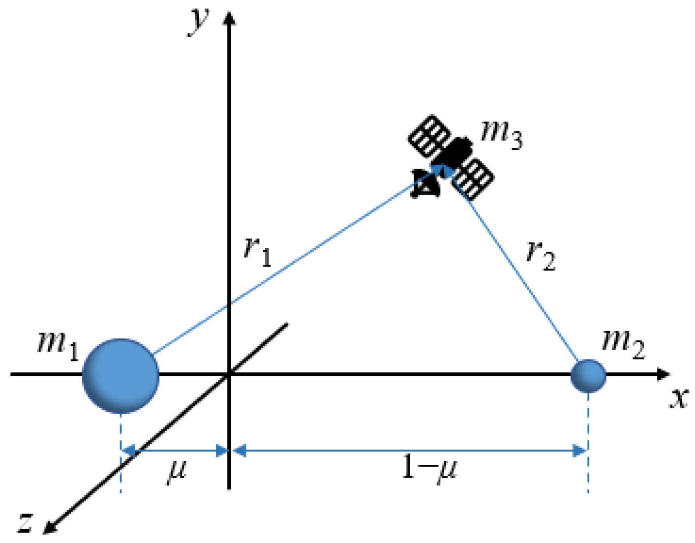
2.1. The Circular Restricted Three-Body Problem

Ganymede has an orbital eccentricity of 0.0013, which is very small; this means that the CR3BP can be used to provide an approximation of Jupiter–Ganymede dynamics. The dynamical model in the CR3BP consists of three bodies, with masses m1, m2, and m3. The third body m3 is massless compared to the two primaries, m1 and m2, without the loss of generality, assuming m1 > m2. The CR3BP assumes that two primary bodies are moving in a circular orbit about their common barycenter and that the motion of m3 is dominated by the gravitational attractions of them. Conventionally, the system is normalized, such that both the distance between m1 and m2, LU, and the mean motion of the primaries, WU, are constant and equal to unity, which means that the orbital period of m2 is 2π time units. In addition, let μ denote the ratio of the mass of the secondary body to the total mass, so that the first and secondary primaries’ masses are nondimensional and equal to 1 − μ and μ, respectively. The motion of the third body is then described using a normalized dimensionless synodic system. The synodic system is a rotating coordinate system, with its origin at the barycenter of the primaries, an x-axis directed from the origin in a direction away from the primary, a y-axis aligned with the direction of the velocity vector of the secondary, and a z-axis completing the right-handed coordinate system, as depicted in Figure 1. In this rotating frame, the equations of motion for the third body are written thus, as seen in [25]:
{ x ¨ 2 y ˙ = U x y ¨ + 2 x ˙ = U y z ¨ = U z
where U denotes the pseudo-potential expressed thus, as seen in [25]:
U = x 2 + y 2 2 + 1 μ r 1 + μ r 2
with r1 and r2 defined thus, as seen in [25]:
r 1 = ( x + μ ) 2 + y 2 + z 2 r 2 = ( x 1 + μ ) 2 + y 2 + z 2 .
Equation (1) admits an energy-like integral of the motion, called the Jacobi constant, which serves to characterize the families of trajectories and is written thus, as seen in [25]:
J = x 2 + y 2 + 2 ( 1 μ ) r 1 + 2 μ r 2 + μ ( 1 μ ) ( v x 2 + v y 2 + v z 2 ) .
To describe the simplified Jupiter–Ganymede system, μ = 7.8063 × 10⁻⁵, LU = 1.0704 × 10⁶ km and WU = 1.0164 × 10⁻⁵ rad/s are used in this work.

2.2. Numerical Methods

Solutions that are symmetric about the x-axis and the xz plane are evident from the symmetry in Equation (1). For the application of the periodicity theorem proposed by Roy and Ovenden [26] for the CR3BP, it is immediately obvious that a trajectory that perpendicularly crosses the xz plane or the x-axis twice is a closed periodic orbit. Therefore, there are actually three possible types of symmetric periodic solutions in the CR3BP: an axis-symmetric (AS) orbit, which has two perpendicular crossings of the x-axis, a plane-symmetric (PS) orbit, which has two perpendicular crossings of the xz plane, and a doubly symmetric (DS) orbit, which satisfies an AS configuration and a PS configuration [27,28,29]. In this work, DROs, which belong to the AS orbits in the planar CR3BP, are investigated.
Let [x0, 0, 0, 0, vy0, 0]T denote the initial state of a DRO, where y0 = 0, z0 = 0, vx0 = 0, and vz0 = 0 indicate that the planar orbit perpendicularly crosses the plane y = 0 at the initial time. To obtain a periodic, symmetric, and planar orbit, this initial state will be propagated forward in time for half a period, when this orbit should perpendicularly cross the plane y = 0 once again. In this work, the MATLAB function, ODE45, is employed to solve the dynamical differential equations of DR3BP. Specifically, we set both the absolute and relative error tolerance of 10−10 and use the “Events” option to specify that the integration terminates at a zero where the event function is increasing. The steps of numerical computation that are used to achieve a family of symmetric periodic orbits are summarized as follows. First, given the initial position x0, the initial velocity vy0 can be calculated in the two-body system; thus, we have the initial guess for a starting point. Next, dichotomy or differential correction can be used to correct vy0, such that the orbit will pass perpendicularly through the plane y = 0; thus, the first orbit is found. Then, by means of numerical continuation with respect to x0, a family of orbits can be obtained.

2.2.1. Dichotomy

Since only one variable needs to be adjusted, we can use dichotomy to establish a sufficiently precise initial value. Generally, we choose 0.1 or 0.01 as the length of the dichotomy interval for the dimensionless variable vy0 after normalization. Unless otherwise stated, the following calculations and drawings are carried out in the normalized coordinate system. Qualitatively, when the probe passes through the plane y = 0, the centripetal or centrifugal trend of the probe can be determined by judging the direction of the velocity vector (or the direction of vx), as shown in Figure 2, where the middle orbital is perpendicular to the x-axis, the left orbital has vx < 0, and the right orbital has vx > 0. Then, the initial velocity value is corrected by dichotomy. This method has a high convergence speed for calculating two-dimensional periodic orbits with good symmetry, but its disadvantages are that the convergence range is small, the input guess initial value cannot differ too much from the “exact value”, and the length of the dichotomy interval cannot be too large. When the problem is extended to three dimensions, the dichotomy method fails. At that time, a shooting correction method for the state transition matrix is still needed.

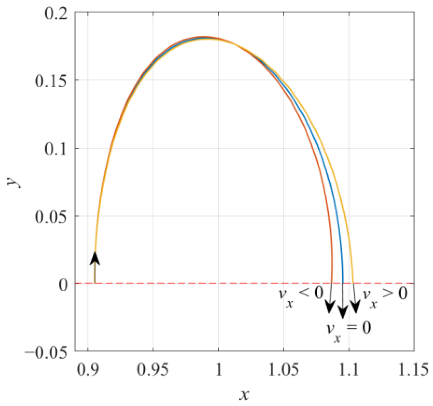
2.2.2. Differential Correction

The state transition matrix (STM), the product of which, with the state vector at an initial time t0, gives the state vector at a later time t, is denoted by Φ(t, t0) here. Considering the three-dimensional orbits that are symmetric about the plane y = 0, let [x0, 0, z0, 0, vy0, 0]T denote the initial state of the orbit. If correction is not performed, the state when the probe passes through the plane y = 0 can be expressed as [x, 0, z, vx, vy, vz]T. When fix z0 and correct x0 and vy0, the first-order relationship between the free variables and the boundary values at half a period can be expressed thus, as seen in [30]:
[ δ v x , T / 2 δ v z , T / 2 ] = [ φ 41 v ˙ x φ 21 y ˙ φ 45 v ˙ x φ 25 y ˙ φ 61 v ˙ z φ 21 y ˙ φ 65 v ˙ z φ 25 y ˙ ] [ δ x 0 δ v y 0 ]
where φij denotes the element in the ith row and the jth column of Φ(T/2, t0). Based on this relationship, the initial condition of a periodic orbit is calculated when vx,T/2 and vz,T/2 are reduced to a defined small value by several iterations. If the problem is a two-dimensional one, Equation (5) can be simplified as:
δ v x , T / 2 = ( φ 45 v ˙ x φ 25 y ˙ ) δ v y 0 .

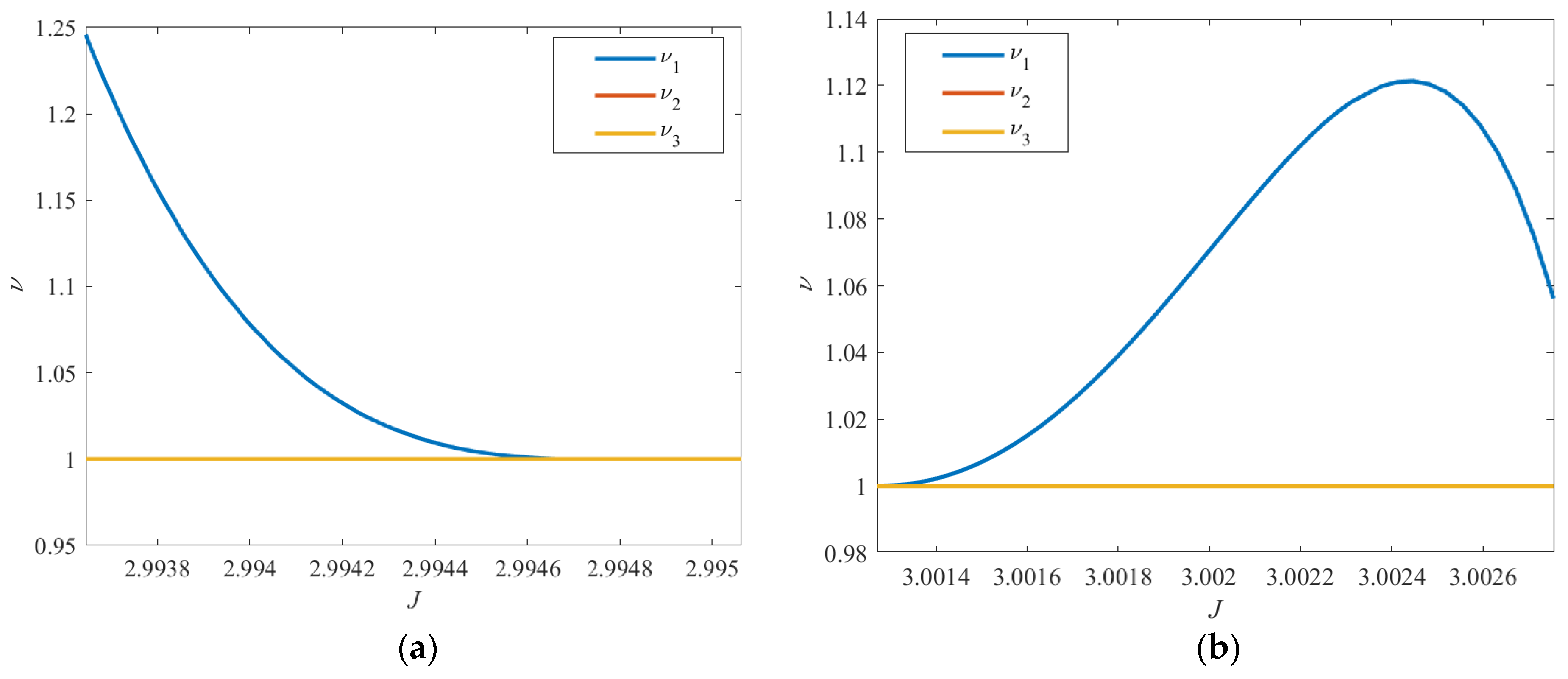
2.3. Orbital Stability

The monodromy matrix is the STM evaluated after one period along a periodic solution, written as M = Φ(t0 + T, t0). For more details of the monodromy matrix, readers are referred to Ref. [31]. In the CR3BP, the second-order system possesses three degrees of freedom and, thus, M is defined in terms of six eigenvalues. First, because the monodromy matrix is a symplectic map, if λi is an eigenvalue of the matrix M, then 1/λi is also an eigenvalue. Second, because the monodromy matrix is associated with a periodic solution, at least one unity eigenvalue will always exist. Furthermore, the fact that eigenvalues of matrix M must come in reciprocal pairs results in at least two unity eigenvalues. Thus, the set of eigenvalues from the monodromy matrix for a particular periodic orbit occurs in the form (λ1, 1/λ1, λ2, 1/λ2, λ3, 1/λ3), where λi represents the eigenvalue of M and λ1 = 1/λ1 = 1. The eigenvalues of matrix M are used to assess the stability characteristics of a periodic orbit in a linear sense. The eigenvalue with a magnitude greater than one indicates instability, while the eigenvalue with a magnitude equal to one reflects orbit periodicity, and the eigenvalue with a magnitude less than one indicates stability. Accordingly, the linear stability of an orbit can be described by stability indices, which are defined thus, as seen in [9,32,33]:
ν i = 1 2 ( λ i + 1 λ i ) , i = 1 , 2 , 3 .
If all the stability indices are equal to unity, the orbit is said to be linearly stable and possesses neither stable nor unstable manifolds; if any stability index is greater than unity, the orbit is considered unstable, and invariant manifolds that approach and depart from the periodic orbit will exist. Evidently, the stability index that corresponds to the two unity eigenvalues is always equal to unity. Therefore, merely considering the other two indices, in the case where they are both equal to unity, the linear instability of the orbit is order zero; in cases where they are both greater than unity, the linear instability of the orbit is order two; otherwise, the linear instability of the orbit is order one. That is to say, the linear instability in this system can be of orders zero, one, or two. The order of orbital instability yields the linear stability level of the orbits. A periodic orbit with instability order zero is the most stable orbit, in a linear sense.

2.4. Bifurcations

In dynamical systems, a change in the stability of the periodic orbits results in a bifurcation. There are three distinct ways in which the stability can change, denoted by a tangent bifurcation, period-doubling bifurcation, and secondary Hopf bifurcation, respectively. In addition, other types of bifurcation occur along the original solution without a change in the order of instability, such as period-multiplying bifurcations and a modified secondary Hopf bifurcation. For more details on bifurcations, readers are referred to Ref. [34]. The stability of a periodic orbit reflects the behavior of nearby trajectories; thus, monitoring the eigenvalues of the monodromy matrix corresponding to each periodic orbit in a family is a good method by which to detect and characterize the local bifurcations.
In 1969, Broucke [35] introduced an alternative method to discuss stability, based on two stability coefficients of the orbit, α and β:
α = ( λ 2 + 1 λ 2 + λ 3 + 1 λ 3 ) = 2 Tr ( M ) β = 1 2 [ α 2 ( λ 2 2 + 1 λ 2 2 + λ 3 2 + 1 λ 3 2 ) ] = 1 2 [ α 2 + 2 Tr ( M 2 ) ]
In this technique, four nontrivial eigenvalues of the monodromy matrix for each family member are fully defined by the scalars α and β. The Broucke stability diagram in Figure 3a offers insight into the orbital stability in the α-β plane. A more informative stability diagram [34], based on the Broucke stability diagram, is constructed as shown in Figure 3b. Each periodic orbit may be represented by a point in Figure 3b; thus, a curve that illustrates a family of periodic orbits can be drawn. Bifurcations occur when this curve intersects those in Figure 3b and bifurcation points, namely, intersections are found. In Table 1, bifurcation types are described with the equations of curves in Figure 3b.

2.5. Invariant Manifolds

Invariant stable and unstable manifolds are considered in this work. If the probe moves on the stable manifolds of a periodic orbit, it will asymptotically approach that orbit without providing external energy; if it moves on unstable manifolds, it will asymptotically depart from that orbit without providing external energy. Accordingly, invariant manifolds can be leveraged to design low-energy orbital transfer. Consider a periodic orbit that possesses one pair of stable and unstable eigenvalues, indicated by |λs| < 1 and |λu| > 1. Correspondingly, there is a pair of stable and unstable eigenvectors, indicated by es and eu. The invariant manifolds corresponding to the propagations of es and −es are stable manifolds, while those corresponding to the propagations of eu and −eu are unstable manifolds. For a point of an unstable orbit, xo, we introduce a small disturbance in the direction of the corresponding eigenvectors, thereby producing initial conditions for the stable and unstable manifolds, xs,0 and xu,0, respectively:
x s , 0 = x o ± ε e s x u , 0 = x o ± ε e u
where ε is a sufficiently small real-valued number. The stable and unstable manifolds at this point can be computed by propagating the initial conditions forward and backward in time, respectively. Note that when dissipative forces are considered, the manifold obtained above needs to be modified in the initial value, or halfway, to achieve the transfer orbit between the target bodies. If we discretize the orbit into numerous points and repeat the steps above, then the stable and unstable manifold structures are obtained [36,37]. For orbits that have complex geometric configurations, such as period-multiplying orbits, drawing manifolds directly is detrimental to subsequent analysis; therefore, a Poincaré section is employed to delineate the manifold structures in this case.

3. The Ganymede DRO Family and Its Bifurcations

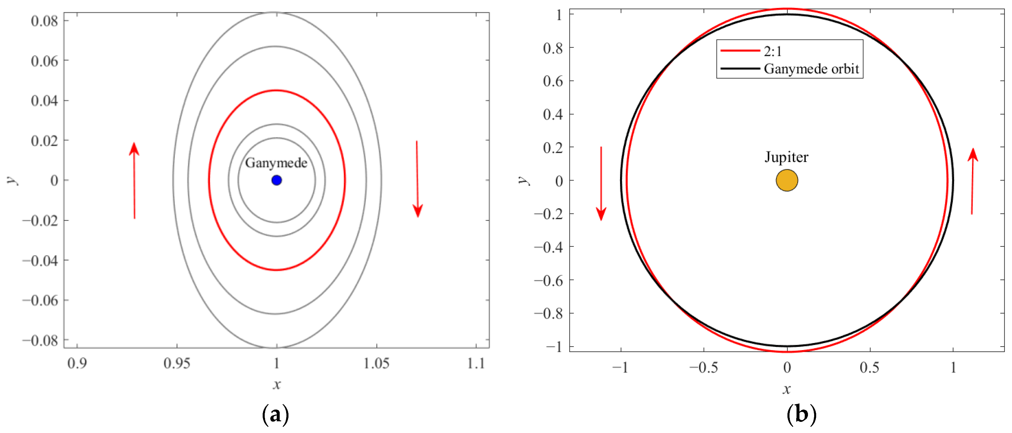
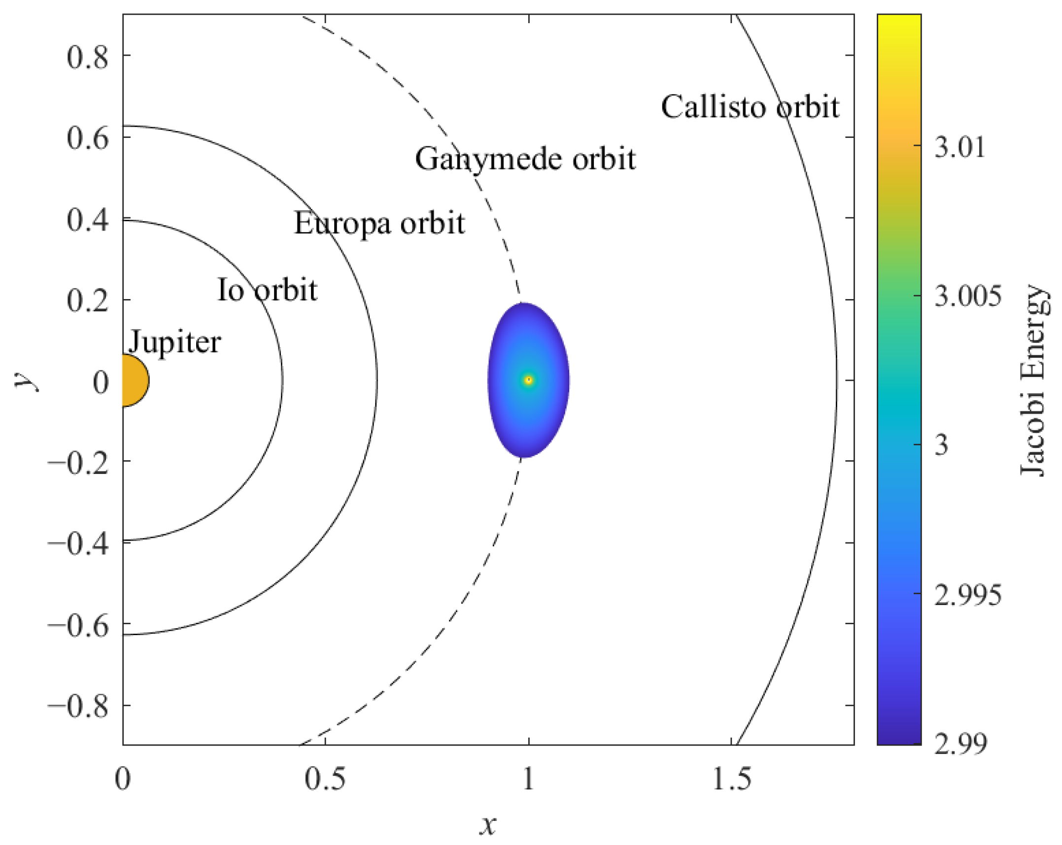
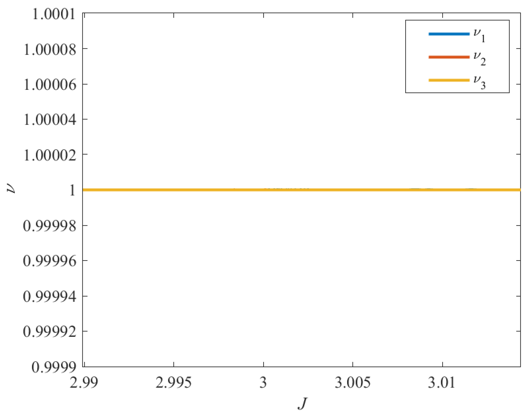
3.1. The DRO Family and Its Linear Stability

A resonant DRO (2:1) and its direction of motion in the synodic frame and in the Jupiter-centered inertial frame are shown in red in subgraphs (a) and (b) of Figure 4, respectively. It is evident that the DRO around the secondary body is in a direction opposite to the direction of the secondary body orbiting around the barycenter when viewed in the rotating frame, and orbits in a prograde direction following the secondary body when viewed in the inertial frame; hence, it is called a distant retrograde orbit (DRO).
Considering the positions and perturbations of the other three Galilean moons, the DRO family whose initial position x0 covers from 0.9 to 0.995 with an interval of 0.0005 is calculated, as shown in Figure 5. Each color of orbit indicates each Jacobi constant value, as specified by the color bar on the right. Jupiter and the four Galilean moons’ orbits around Jupiter are drawn to real proportion. It is apparent that the DROs orbiting closer to Ganymede possess higher Jacobin constant values, which can be as high as the Jacobin constant values for L1 and L2. Figure 6 shows that the three stability indices of DROs are equal to unity; namely, all the orbits of this family are linearly stable.

3.2. Bifurcations of DROs

As indicated by the stability indices, DROs cannot be targeted with a low-energy transfer along stable and unstable manifolds, as with unstable orbits in the CR3BP. Therefore, alternative strategies are necessary to understand and exploit the natural flows in the vicinity of the DROs. In dynamical systems, a bifurcation may result in a new family of periodic orbits intersecting with the current family, and it is in this new family that useful stable and unstable manifold structures may arise. Bifurcation theory is applied to give a further investigation of the dynamical structures in the DRO vicinity, providing insight into the complex trajectory behavior in this region.

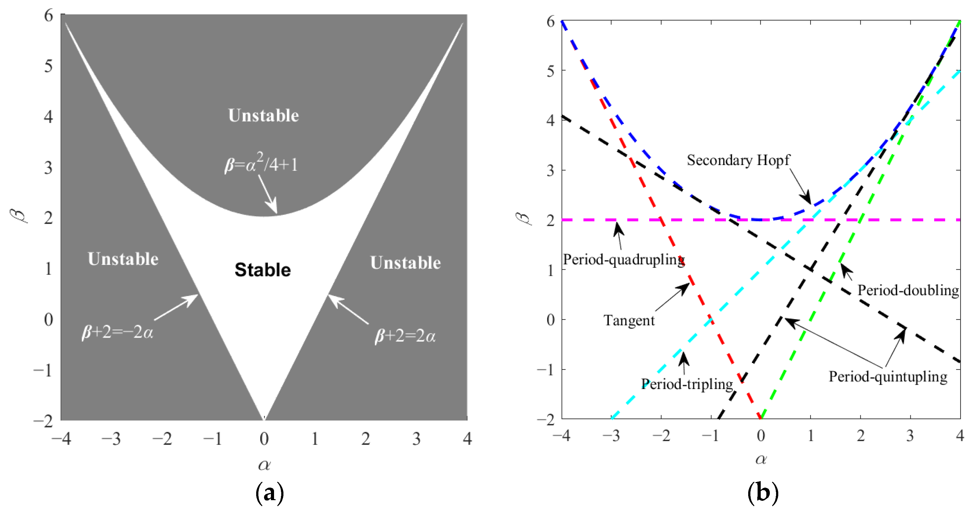
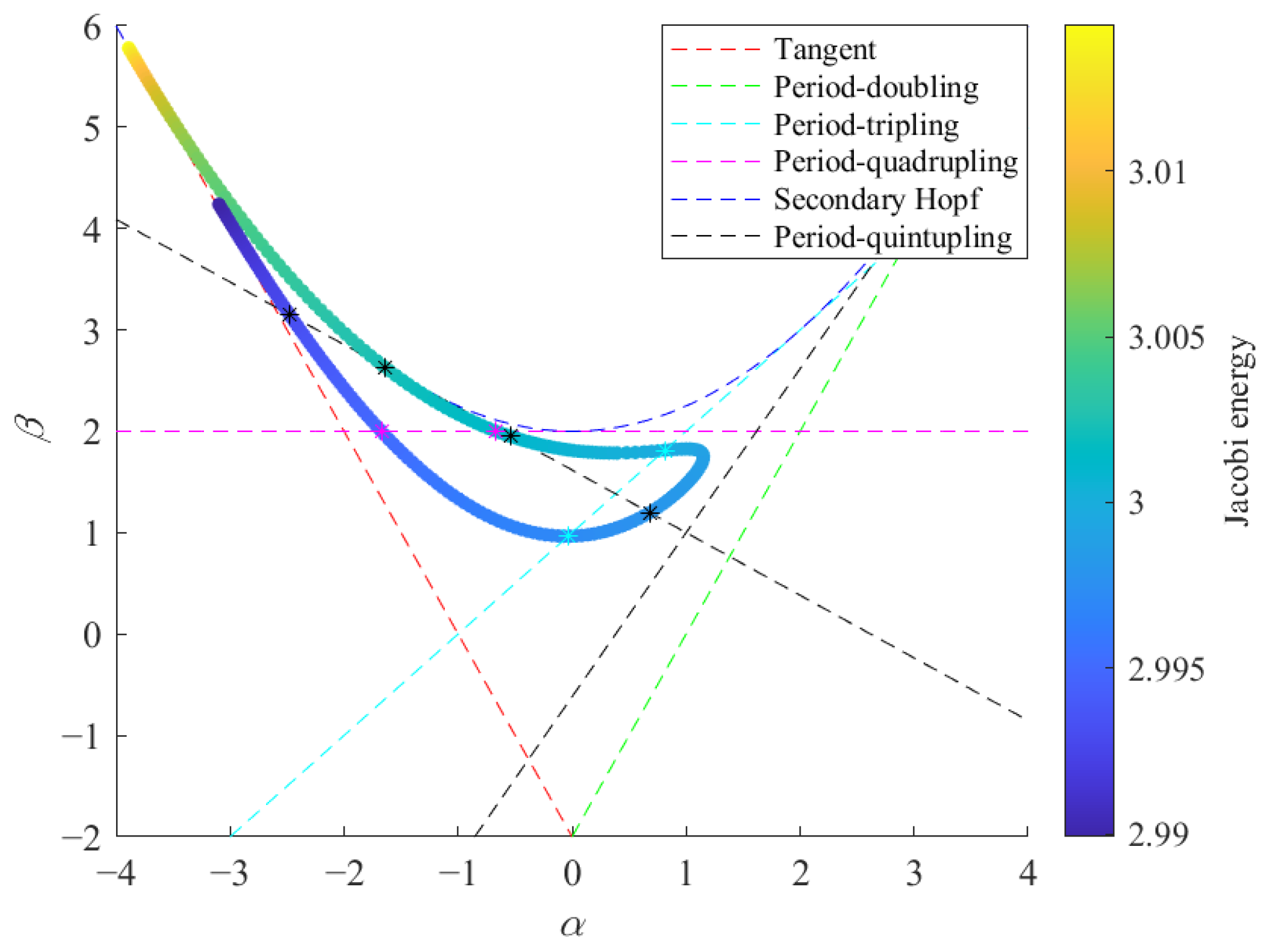
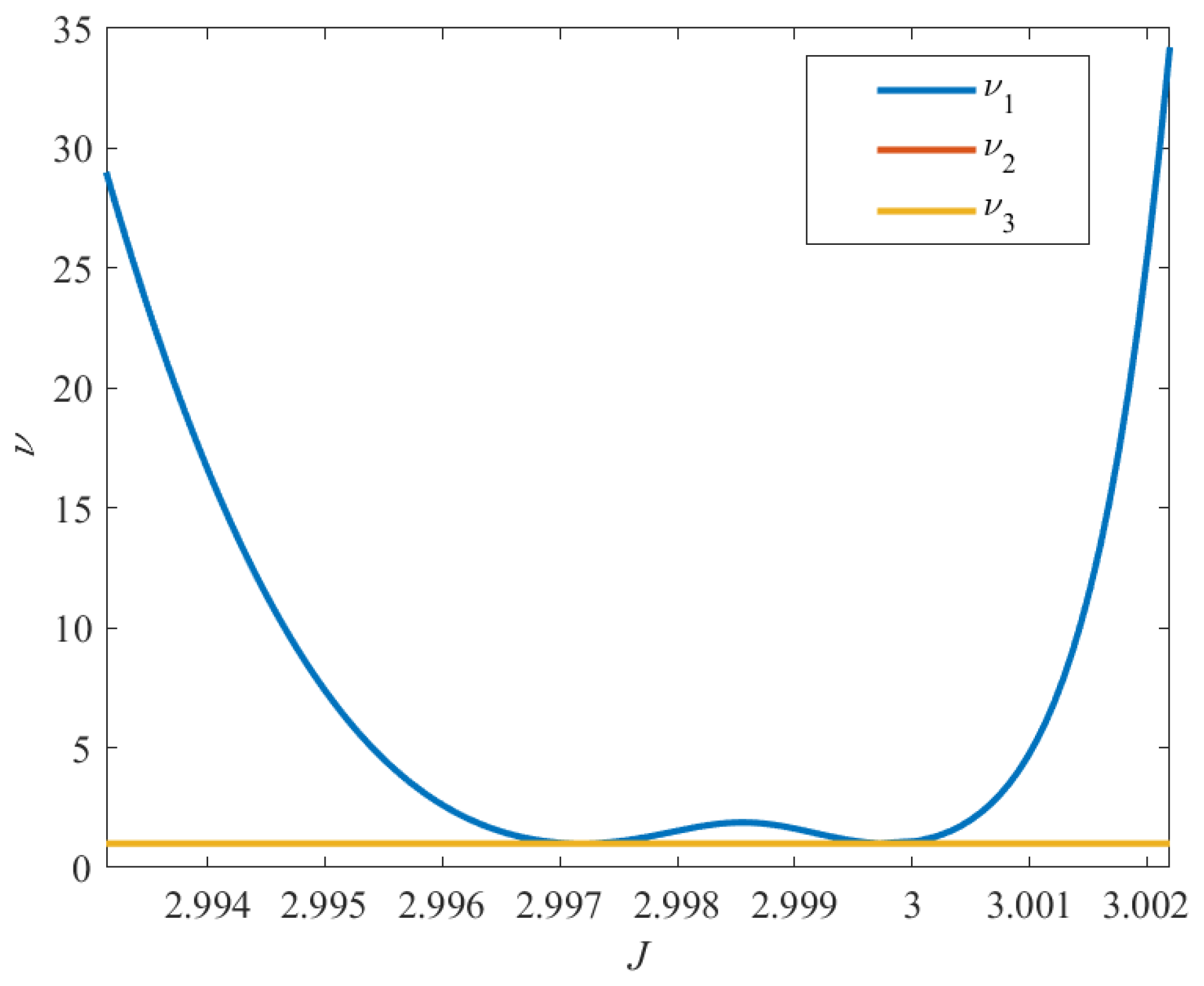
3.2.1. DRO Stability Diagram

In Figure 7, a colorful curve is plotted on the stability diagram that corresponds to the DRO family. The color of each point indicates the Jacobi constant value for this orbit. In this figure, colored asterisks reflect the bifurcation points that correspond to bifurcations with the same color. Evidently, period-tripling, period-quadrupling, and period-quintupling bifurcations occur. To easily recognize these bifurcating orbits and the corresponding families to which they belong, a naming convention [33] for these new families is necessary. For period-multiplying bifurcations, the naming format is defined as follows: “PmDROn”, where “Pm” refers to the order of the period-multiplication (e.g., period-tripling is reflected as m = 3), and “n” denotes a sub-family identifier (i.e., for multiple bifurcations of the same type, the first family, in order of increasing initial position x0, is labeled n = 1, the second family is labeled n = 2, etc.). Accordingly, new families originating from period-tripling bifurcation are named P3DRO1, P3DRO2, and P3DRO3; new families originating from period-quadrupling bifurcation are named P4DRO1 and P4DRO2; new planar families originating from period-quintupling bifurcation are named P5DRO1 and P5DRO2. Employing the numerical methods stated in the previous section, all the new families of periodic orbits originating at each of these bifurcations are computed. In Section 3.2.2, Section 3.2.3 and Section 3.2.4, the bifurcating orbits and their stability are investigated to find the underlying unstable manifold structures for low-energy transfer design between DROs.

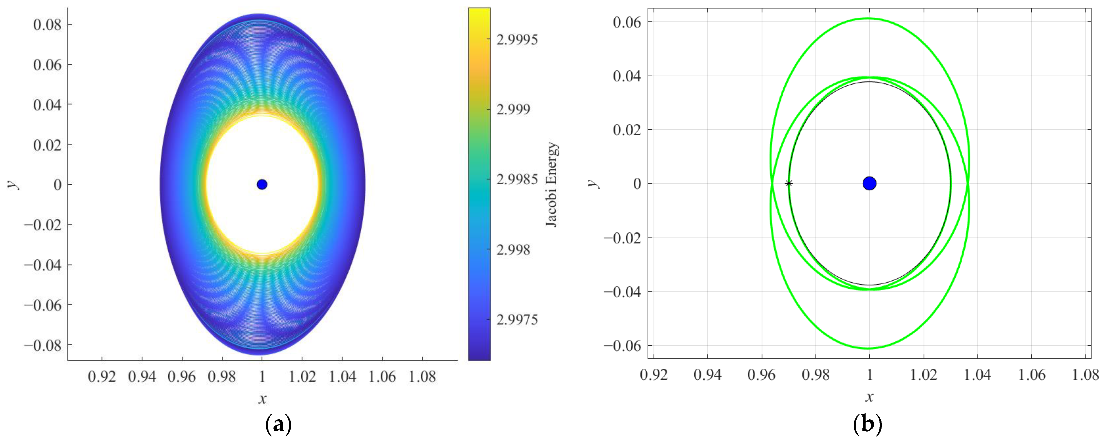
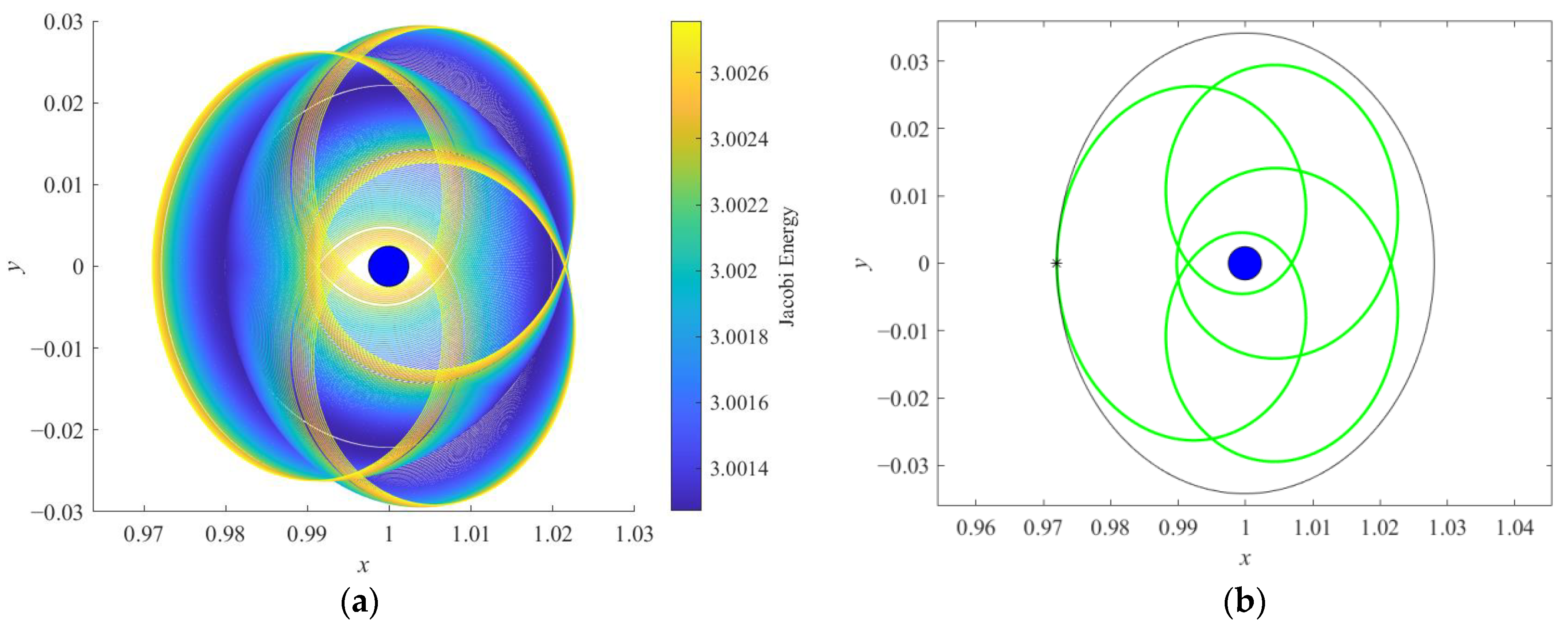
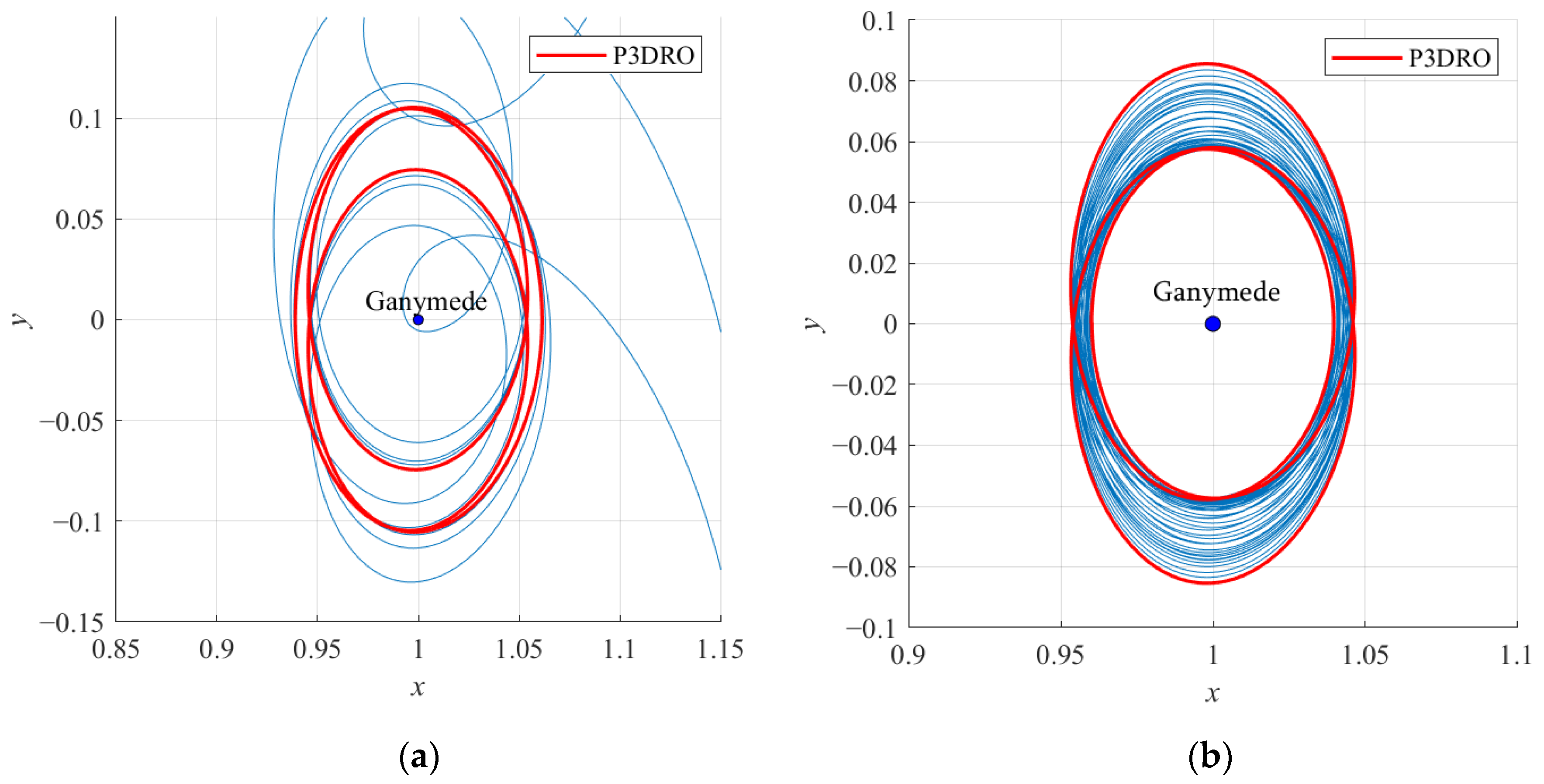
3.2.2. Period-Tripling Bifurcation

The P3DRO families and their linear stability are studied in this subsection. The characteristics of orbits in the P3DRO1, P3DRO2, and P3DRO3 families are illustrated in Figure 8a, Figure 9a, and Figure 10a, respectively. In Figure 8b, Figure 9b, and Figure 10b, a member from each of these new families is computed and plotted in the synodic system to illustrate their complex multi-revolution geometries, along with their unique and distinct characteristics. In each of these figures, an orbit of new periodic families is plotted in green, along with a DRO of the same initial position x0 in black, while Ganymede appears as a blue sphere, and the initial point along each trajectory is marked with an asterisk.
The families of period-tripling bifurcating orbits possess periods that are approximately three times the period of the DROs, and the periods decrease as the orbits approach Ganymede. Each family possesses different levels of Jacobi energy and different geometries. The P3DRO1 family possesses a Jacobi energy of less than 2.9972. Orbits in this family are a long distance from Ganymede, even though they propagate from a position far from Ganymede to a closer one. The P3DRO2 family with a Jacobi energy from 2.9972 to 2.9998 closely approximates a DRO-like motion, albeit periodic, with three Ganymede passes instead of one. The P3DRO3 family possesses a Jacobi energy greater than 2.9998. Some of the larger members of this family offer positions close enough to Ganymede; note that, with a further extension of this family, the members with higher Jacobi energy will pass inside Ganymede’s radius. This property may prove useful in landing or impact missions. Figure 11 presents the stability information of period-tripling bifurcating orbits. Apparently, only the orbits at the bifurcation points are linearly stable, while the other orbits are linearly unstable, with a maximum index from 1 to 35. Accordingly, the unstable P3DRO families can be taken into consideration when designing low-energy trajectories in the vicinity of the DROs.

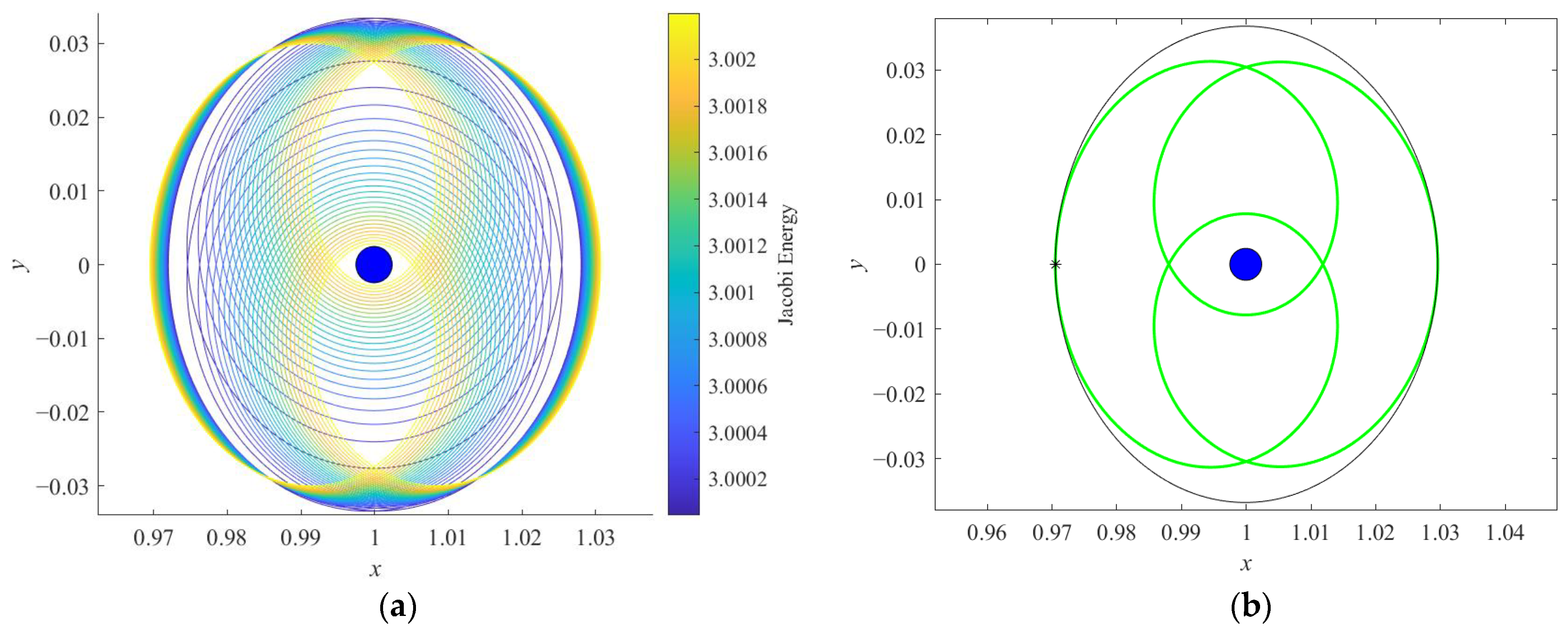
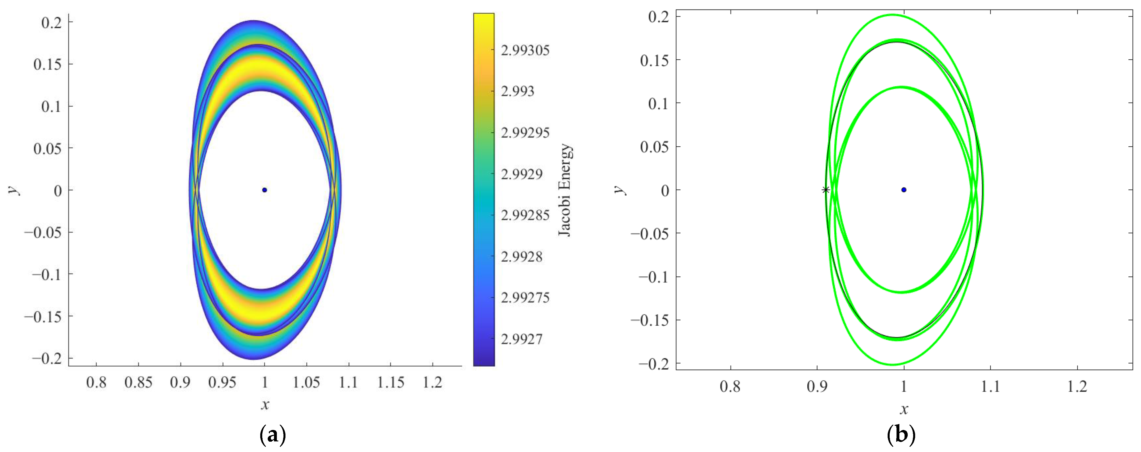
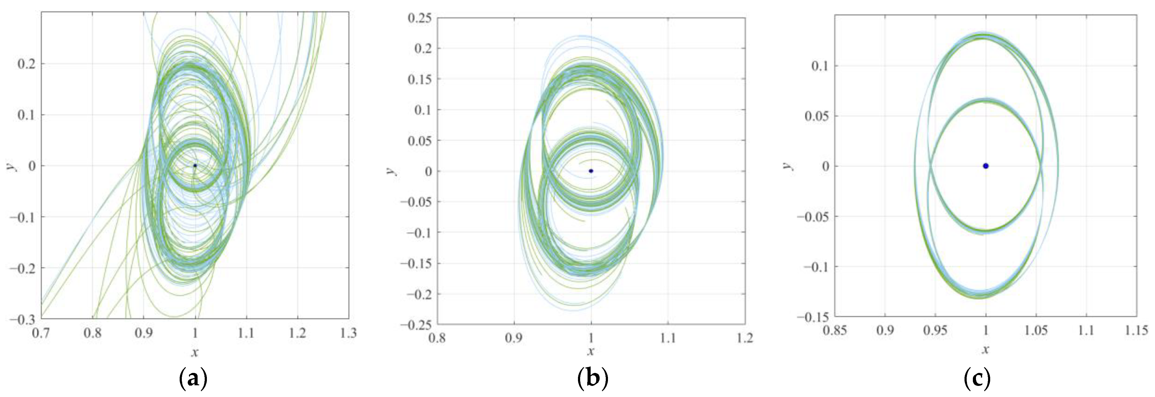
3.2.3. Period-Quadrupling Bifurcation

The P4DRO families and their linear stability are studied in this subsection. The P4DRO1 and P4DRO2 families appear in Figure 12 and Figure 13, following the same convention as the period-tripling bifurcation, respectively. Orbits in the P4DRO1 family possess a Jacobi energy of less than 2.9951, while orbits in the P4DRO2 family possess a Jacobi energy larger than 3.0013. In contrast to the P4DRO1 family, the P4DRO2 family has a smaller size and exists in the vicinity of Ganymede. A range of orbits in the P4DRO2 family can reach within the radius of Ganymede (not pictured here), while the portion plotted here offers a fully low altitude. These new families of periodic orbits that are calculated here are linearly stable or nearly stable, as delineated in Figure 14, which means that there is no manifold structure available by which to design low-energy transfer orbits.

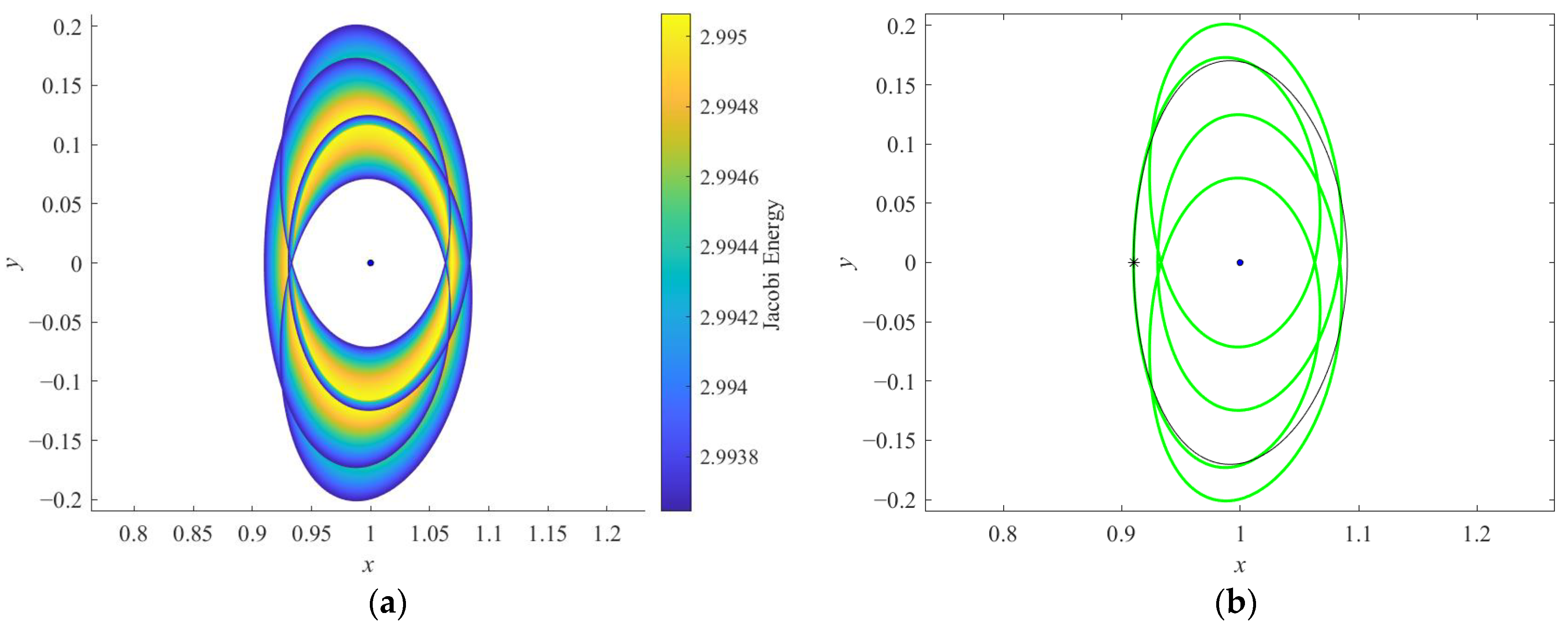
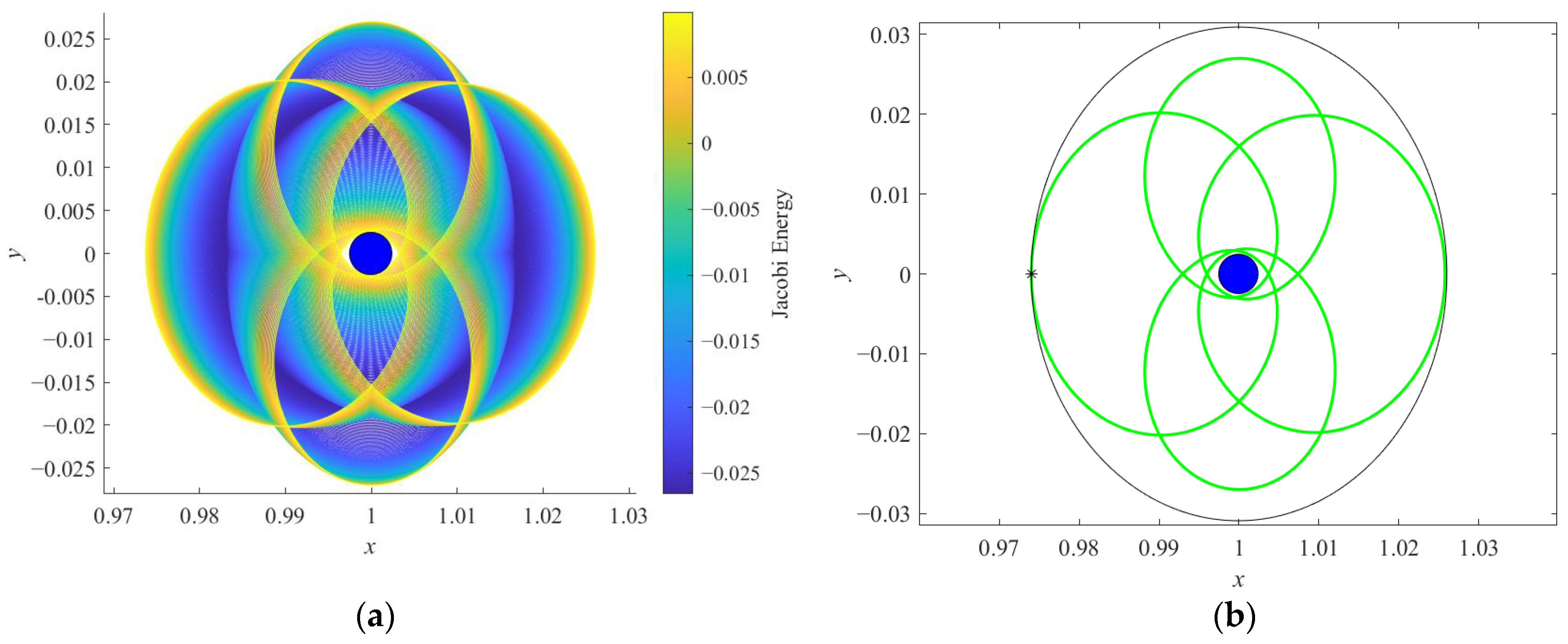
3.2.4. Period-Quintupling Bifurcation

The P5DRO families and their linear stability are studied in this subsection. According to the stability diagram for DROs, two planar families and two three-dimensional families of period-quintupling bifurcating orbits are identified. In this investigation, only two planar families of period-quintupling bifurcating orbits, namely, P5DRO1 with a Jacobi energy of less than 2.9931 and P5DRO2, with a Jacobi energy larger than 3.0023, are discussed. Note that, for the P5DRO2 family, two trajectories of different multi-revolution geometries may exist while sharing the same Jacobi energy. Figure 15, Figure 16 and Figure 17 illustrate the family P5DRO1 and two sub-P5DRO2 families with different structures, respectively. The P5DRO1 family is far from Ganymede, has a larger size, and possesses a low level of Jacobi energy, while the P5DRO2 family has a smaller size, where the orbit sometimes moves very close to Ganymede. A remarkable distinction between the two sub-P5DRO2 is that in the synodic system, the third body orbits Ganymede inward and outward, as shown in Figure 16 and Figure 17, respectively. As indicated in Figure 18, the planar families of period-quintupling bifurcating orbits are linearly stable or nearly stable.

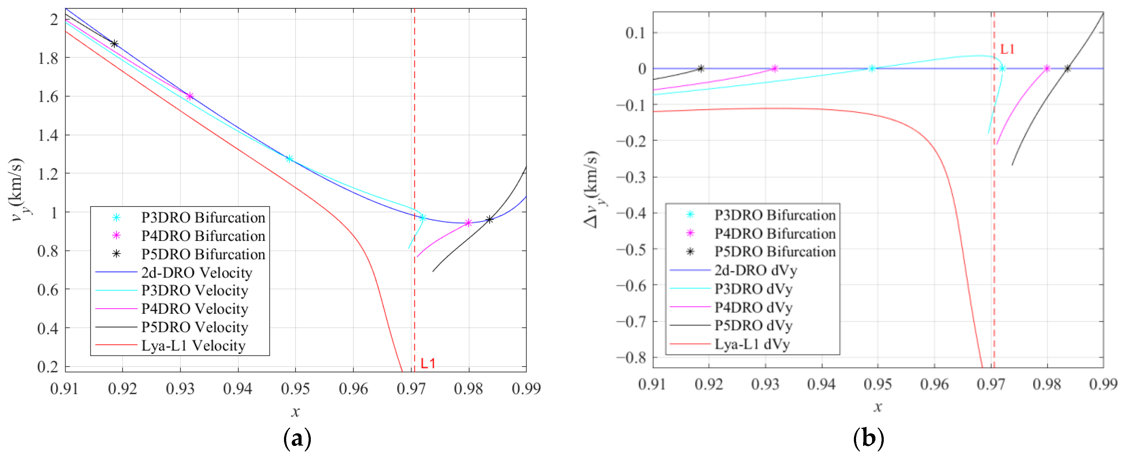
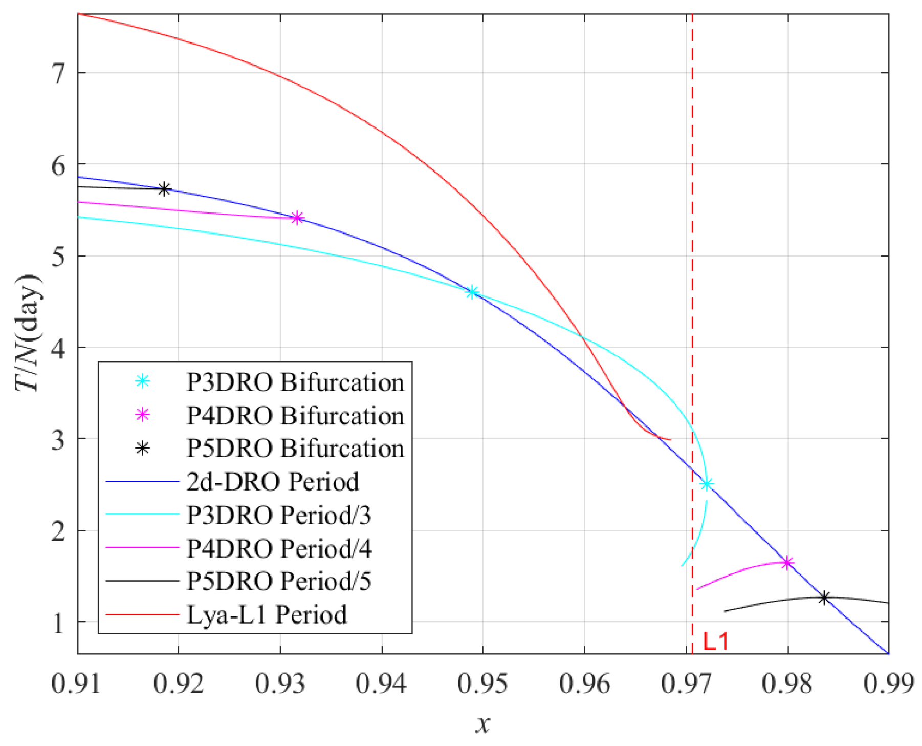
3.3. Analysis of Perturbations

Previous research [38] focuses on the perturbations of the low orbit of Europa (100~400 km of altitude). At this altitude, Europa’s gravitational influence is dominant, while the gravitational influence of other moons is not obvious. The DROs around Ganymede that we are studying are at higher altitudes of more than 3000 km, even reaching 100,000 km. The DROs are also dominated by the gravitational influence of Jupiter and Ganymede. The higher orbits would increase the gravitational influence of Europa or Callisto, especially for the unstable bifurcation orbits of DROs, while the gravitational perturbations of other moons will disrupt the structure of the bifurcation orbits.
In the Jupiter–Ganymede CR3BP system without any perturbation, the DROs around Ganymede are stable. However, because of the special periodic resonance relationship between the Galilean moons and their short period characteristics, the perturbations cannot be ignored for practical missions. Thus, the gravitations of the Galilean moons and the Sun are considered as perturbations in this work, to investigate the time evolution of a massless body orbiting Jupiter. Here, we use an inertial frame with Jupiter at its center, while the Galilean moons and the Sun are moving in circular orbits about the origin of this coordinate system.
The initial condition X0 of a DRO can be calculated in the CR3BP system, then transformed to the inertial system and given the Galilean moons’ and the Sun’s initial phase angles θi0 (i = 1, 2, 3, 4) and θs0, respectively. The DRO affected by their gravitational perturbations can be obtained by propagating X0 forward. One example of perturbed DRO at X0 = [0.9400, 0, 0, 0, 0.13208, 0]T with θi0 = 0 and θs0 = 0 and a propagation time of 1 year is shown in Figure 19. The influence of the Sun’s gravity in the Jupiter system is very small, so the main perturbation influence comes from the other Galilean moons. Meanwhile, the investigated DRO is a considerable distance from the other Galilean moons, as shown in Figure 19b. Therefore, the perturbed DRO remains in a similar trajectory to the DRO, without any perturbation within the given propagation time. When this trajectory crosses the y = 0 plane, the position error in the x-direction is about ±0.0006, actually about ±600 km. The position errors between the perturbed and unperturbed DRO orbits in the x direction at different times are plotted, as shown in Figure 20. It shows that although the perturbed DRO orbit is stable around the original DRO orbit, the orbit position error shows an increasing trend. Therefore, it is still necessary to maintain the orbit in a timely manner.
Furthermore, we consider the motions of period-tripling DRO bifurcating orbits under the gravitational perturbations and find that for some of these orbits, they will quickly move away from the original orbit and diverge outward after being affected by the perturbations (Figure 21a), while some can maintain their orbit for a long period of time without diverging within a certain range, and become quasi-periodic orbits (Figure 21b). This behavior is related to the stability of the orbits, which will be explained briefly in the next subsection. In addition, this is also related to the structure of the orbit. When the altitude relative to Ganymede is higher, the perturbation effect is stronger.

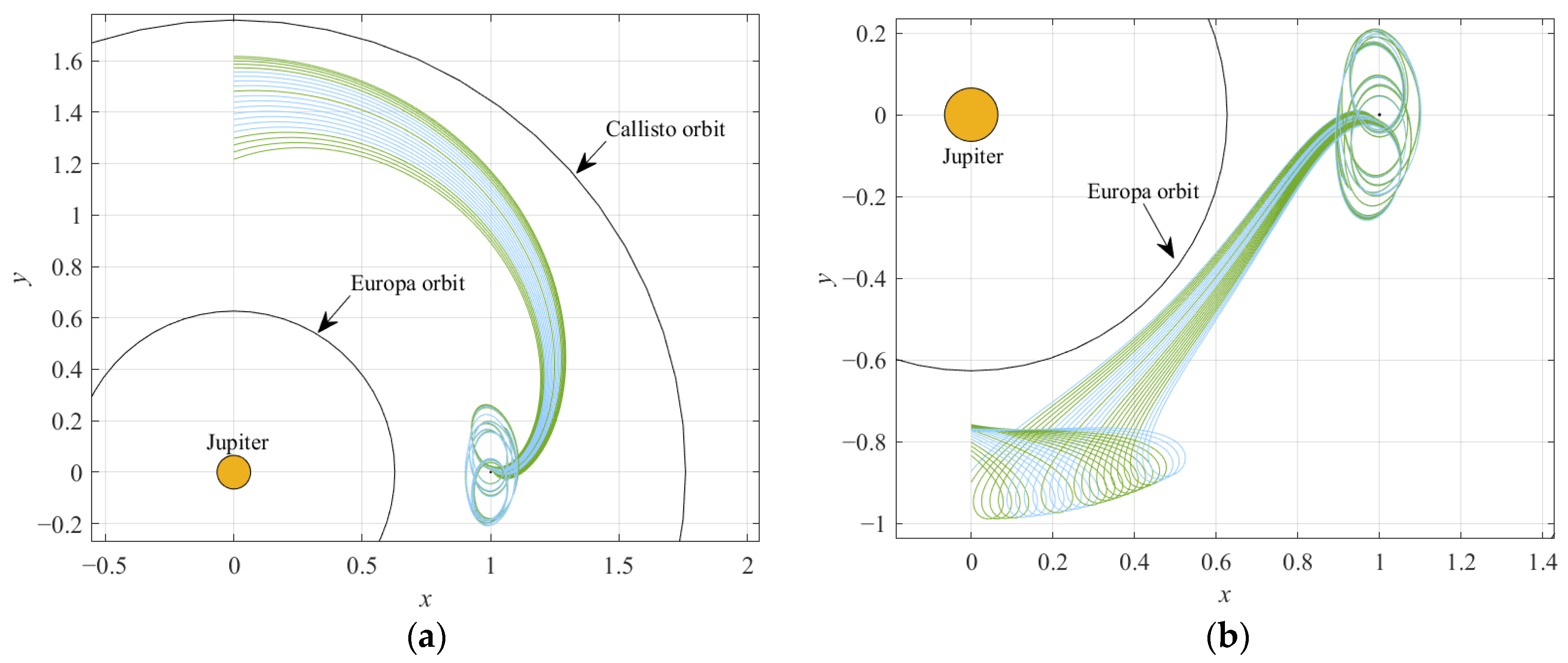
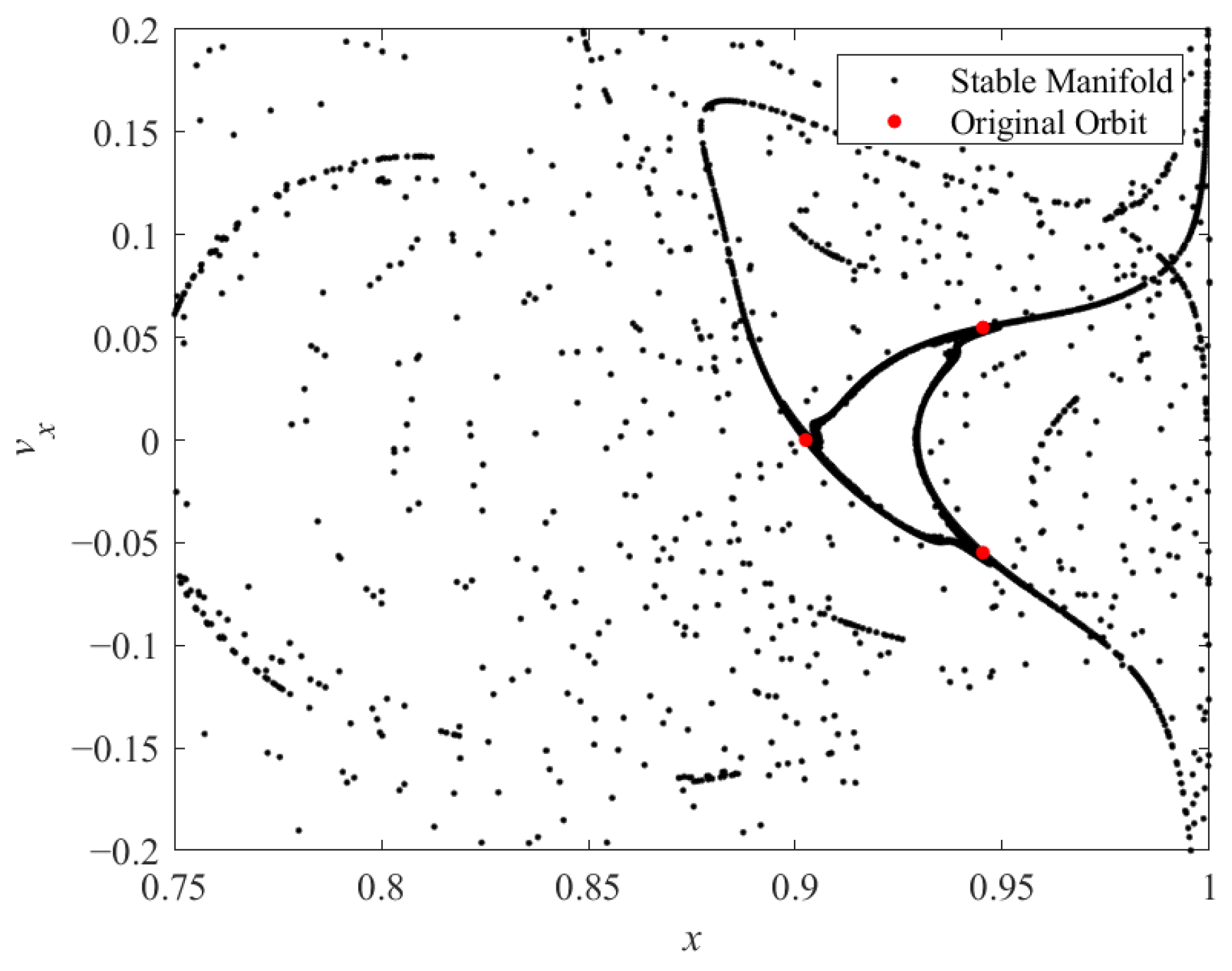
3.4. Manifold Structures

Often leveraged to generate the initial guesses for transfer orbit design in the CR3BP, manifolds offer pathways for approaching and departure from unstable periodic orbits. The stability of period-multiplying bifurcating orbits has been analyzed in the previous subsection. It was found that the P3DRO family possesses the largest range for the maximum stability index. Thus, taking the period-tripling bifurcation as an example, we select different orbits with the maximum stability indices of νmax = 26.2387, 10.1016, and 3.0858, and choose several initial points uniformly distributed on these orbits, then plot their stable manifold structures (ε = 10−4, about 100 km) with two periodic lengths under the CR3BP model, as shown in Figure 22.
This shows that the magnitude of the stability index is directly related to the rate of the departing/approaching flows. Those orbits that possess small stability indices (generally νmax < 5) depart from/approach their original orbits very slowly when affected by small disturbances, which can be considered approximately linearly stable. The larger the maximum stability index, the more significant the manifold structure and the faster it deviates from the original orbit.
Furthermore, we investigated the manifold structures of engineering significance, the methodology for which is mentioned in Section 2.5. We selected a part of stable manifolds near the period-tripling bifurcation orbit (X0 = [0.9025, 0, 0, 0, 0.19642833, 0]T, J = 2.993305); the integration duration is three times that of the original orbital periods. We selected some points on the original orbit for integration, terminating when the orbits crossed the plane x = 0, and drew their stable manifolds. The initial point of integration is selected as the point on the orbit when the initial value of the original orbit runs for 1.4~1.7 days; their stable manifold structures are shown in Figure 23a. The initial point of integration was selected as the point on the orbit when the initial value of the original orbit runs for 11.0~11.4 days; their stable manifold structures are shown in Figure 23b. The manifolds of these parts of the orbit will come close to the orbit of Europa or Callisto after 20~30 days, so there is the possibility of a fast low-energy transfer between the Galilean moons.
Since the manifold structures of the period-multiplying bifurcation orbits are relatively complex, we use a Poincaré section to draw the coordinates of the stable manifold crossing the plane y = 0, as shown in Figure 24, with coordinates x and vx. The red points in this figure represent the periodic orbit itself. With this information, suitable points can be selected as the starting point, according to the engineering requirement for transfer orbit design.
Figure 25 shows the difference in velocity between the period-multiplying bifurcating orbits and DROs sharing the same initial positions. Figure 26 shows the average period of the period-multiplying bifurcating orbits and the period of DROs. Existing studies usually considered using the horizontal Lyapunov orbits (HLOs) near L1 or L2 to transfer to DROs. From this, we can see that the difference between the initial velocities of the DRO and period-tripling bifurcating orbit is smaller than that between the DRO and Lyapunov orbit. This means that the velocity increment required to enter or leave the DRO via the period-multiplying bifurcating orbits is smaller, and the probe can still have greater energy. At the same time, although the average period of the period-multiplying bifurcating orbits is shorter in most cases, their orbital periods increase almost in multiples; thus, the overall transfer time may be longer. Therefore, trade-offs should be made based on the requirements of the practical mission.
As mentioned above, a portion of the P3DRO family shows obvious instability, and the manifolds near the orbit can be used to design the trajectory entering or leaving the DRO. Note that the period-tripling bifurcation terminates near L1; hence, the manifolds of period-quadrupling and period-quintupling bifurcation or other transfer methods should be considered when a lower-altitude orbit from Ganymede is needed. In addition, considering the difference in energy levels between the different Galilean moons, the manifold structures of the period-multiplying bifurcating orbits can be spliced with the manifold structures of Lyapunov orbits to design low-energy transfers.

4. Conclusions

This paper focuses on investigating the characteristics of DROs and higher-period orbits in the Jupiter–Ganymede system. Bifurcation theory was chosen to detect new families of higher-period orbits near to the DROs. Orbital stability and the invariant manifolds of DROs and higher-period orbits were investigated, based on stability indices and manifold theory, respectively. Then, we further investigated the possibility of approaching/departing from the DROs by means of stable/unstable manifolds in the period-multiplying bifurcating orbits. We found that the DRO family is strongly stable in the Jupiter–Ganymede CR3BP, which is verified through a perturbation model, taking the gravitational perturbations of the other three Galilean moons and the Sun into account. This result indicates that the DROs in the Jupiter–Ganymede system can move nearer the desired orbit for a long time, with negligible fuel consumption for regular orbital corrections, yielding potential applications in orbiting and exploring the Galilean moons. For example, the DROs could be used to place a long-term probe to observe the activity of celestial bodies in the Jupiter system and to build and refine the ephemeris model of the Jupiter system. In addition, among the period-multiplying bifurcating orbits studied in this work, the period-tripling bifurcation was found to have the widest distribution and strongest instability. Therefore, low-energy transfers for DROs can be designed by using the invariant manifold structures near the period-tripling bifurcation. Our preliminary results show that orbital transfer using the period-multiplying bifurcating orbits requires a velocity increment that is less than when using the horizontal Lyapunov orbits, but correspondingly, the transfer time may be longer. Based on this characteristic, some low-energy transfers can be designed by splicing the manifolds of the period-multiplying bifurcating orbits and the horizontal Lyapunov orbits. The discovery of unstable period-multiplying orbits around the DROs also implies the feasibility of a low-energy manifold-to-manifold trajectory that passes by the major moons of Jupiter. For these possibilities, orbiting and exploring missions from DROs around the Galilean moons can be further designed, and low-energy transfer in the vicinity of DROs in a higher-fidelity ephemeris model can be further investigated.

Author Contributions

Q.L. completed the computation of orbits and the analysis of orbital stability, conceived the paper, and wrote most of it; Y.T. completed the computation of orbits and the verification in a perturbation model, analyzed the application of manifold structures, and wrote a small part of the paper; F.J. supervised the overall work, and reviewed and modified the paper. The academic contributions of Q.L. and Y.T. are equally important. All authors have read and agreed to the published version of the manuscript.

Funding

This work was supported by the National Natural Science Foundation of China (Grants. U21B2050 and 12022214) and the Student Research Training project of Tsinghua University.

Institutional Review Board Statement

Not applicable.

Informed Consent Statement

Not applicable.

Data Availability Statement

The data presented in this study are available on request from the corresponding author.

Conflicts of Interest

The authors declare no conflict of interest.

References

  1. Hénon, M. Numerical Exploration of the Restricted Problem 5, Hill’s Case: Periodic Orbits and Their Stability. Astron. Astrophys. 1969, 1, 223–238. [Google Scholar]
  2. Brophy, J.R.; Friedman, L.; Culick, F. Asteroid Retrieval Feasibility. In Proceedings of the 2012 IEEE Aerospace Conference, Big Sky, MT, USA, 3–10 March 2012; pp. 1–16. [Google Scholar]
  3. McGuire, M.L.; Strange, N.J.; Burke, L.M.; McCarty, S.L.; Lantoine, G.B.; Qu, M.; Shen, H.; Smith, D.A.; Vavrina, M.A. Overview of the Mission Design Reference Trajectory for NASA’s Asteroid Redirect Robotic Mission. In Proceedings of the AAS/AIAA Astrodynamics Specialist Conference, Stevenson, WA, USA, 23 October 2017. [Google Scholar]
  4. Howell, S.M.; Pappalardo, R.T. NASA’s Europa Clipper-a mission to a potentially habitable ocean world. Nat. Commun. 2020, 11, 1–4. [Google Scholar] [CrossRef] [PubMed]
  5. Grasset, O.; Dougherty, M.K.; Coustenis, A.; Bunce, E.J.; Erd, C.; Titov, D.; Blanc, M.; Coates, A.; Drossart, P.; Fletcher, L.N.; et al. jUpiter iCy moons Explorer (JUICE): An ESA mission to orbit Ganymede and to characterize the Jupiter system. Planet. Space Sci. 2013, 78, 1–21. [Google Scholar] [CrossRef]
  6. Kawakatsu, Y.; Kuramoto, K.; Ogawa, N.; Ikeda, H.; Mimasu, Y.; Ono, G.; Sawada, H.; Yoshikawa, K.; Imada, T.; Otake, H.; et al. Mission concept of Martian Moons eXploration (MMX). In Proceedings of the 68th International Astronautical Congress, Adelaide, Australia, 25–29 September 2017. [Google Scholar]
  7. Baresi, N.; Dell’Elce, L.; Cardoso dos Santos, J.; Yasuhiro, K. Orbit Maintenance of Quasi-Satellite Trajectories via Mean Relative Orbit Elements. In Proceedings of the 69th International Astronautical Congress, Bremen, Germany, 1–5 October 2018. [Google Scholar]
  8. Hénon, M. Numerical exploration of the restricted problem. vi. hill’s case: Non-periodic orbits. Astron. Astrophys. 1970, 9, 24–36. [Google Scholar]
  9. Broucke, R. Periodic Orbits in the Restricted Three-Body Problem with Earth-Moon Masses; NASA-JPL Technical Report; California Institute of Technology: Pasadena, CA, USA, 15 February 1968. [Google Scholar]
  10. Benest, D. Effects of the mass ratio on the existence of retrograde satellites in the circular plane restricted problem. Astron. Astrophys. 1974, 32, 39–46. [Google Scholar]
  11. Benest, D. Effects of the mass ratio on the existence of retrograde satellites in the circular plane restricted problem. II. Astron. Astrophys. 1975, 45, 353–363. [Google Scholar]
  12. Benest, D. Effects of the mass ratio on the existence of retrograde satellites in the circular plane restricted problem. III. Astron. Astrophys. 1976, 53, 231–236. [Google Scholar]
  13. Hénon, M. Vertical Stability of Periodic Orbits in the Restricted Problem. I. Equal Masses. Astron. Astrophys. 1973, 28, 415–426. [Google Scholar]
  14. Hénon, M. Vertical Stability of Periodic Orbits in the Restricted Problem. II. Hill’s Case. Astron. Astrophys. 1974, 30, 317–321. [Google Scholar]
  15. Bezrouk, C.J.; Parker, J. Long Duration Stability of Distant Retrograde Orbits. In Proceedings of the AIAA/AAS Astrodynamics Specialist Conference, San Diego, CA, USA, 4–7 August 2014. [Google Scholar]
  16. Bezrouk, C.J.; Parker, J. Long term evolution of distant retrograde orbits in the Earth-Moon system. Astrophys. Space Sci. 2017, 362, 176–186. [Google Scholar] [CrossRef]
  17. Lara, M. Nonlinear librations of distant retrograde orbits: A perturbative approach—The Hill problem case. Nonlinear Dyn. 2018, 93, 2019–2038. [Google Scholar] [CrossRef]
  18. Welch, C.M.; Parker, J.S.; Buxton, C. Mission considerations for direct transfers to a distant retrograde orbit. J. Astronaut. Sci. 2015, 62, 101–124. [Google Scholar] [CrossRef]
  19. Demeyer, J.; Gurfil, P. Transfer to Distant Retrograde Orbits Using Manifold Theory. J. Guid. Control. Dyn. 2007, 30, 1261–1267. [Google Scholar] [CrossRef]
  20. Perozzi, E.; Ceccaroni, M.; Valsecchi, G.B.; Rossi, A. Distant retrograde orbits and the asteroid hazard. Eur. Phys. J. Plus 2017, 132, 367–375. [Google Scholar] [CrossRef]
  21. Tan, M.; Zhang, K.; Wang, J. Strategies to capture asteroids to distant retrograde orbits in the Sun–Earth system. Acta Astronaut. 2021, 189, 181–195. [Google Scholar] [CrossRef]
  22. Lam, T.; Hirani, A.N.; Kangas, J.A. Characteristics of transfers to and captures at Europa. In Proceedings of the 16th AAS/AIAA Space Flight Mechanics Meeting, Tampa, FL, USA, 1 December 2006. [Google Scholar]
  23. Lam, T.; Whiffen, G.J. Exploration of distant retrograde orbits around Europa. Am. Astronaut. Soc. Pap. 2005, 120, 135–153. [Google Scholar]
  24. McCarthy, B.P.; Howell, K.C. Leveraging quasi-periodic orbits for trajectory design in cislunar space. Astrodynamics 2021, 5, 139–165. [Google Scholar] [CrossRef]
  25. Howell, K.C. Three-Dimensional, Periodic, ‘Halo’ Orbits. Celest. Mech. 1984, 32, 53–71. [Google Scholar] [CrossRef]
  26. Roy, A.E.; Ovenden, M.W. On the Occurrence of Commensurable Mean Motions in the Solar System: The Mirror Theorem. Mon. Not. R. Astron. Soc. 1955, 115, 296–309. [Google Scholar] [CrossRef]
  27. Robin, I.A.; Markellos, V.V. Numerical determination of three-dimensional periodic orbits generated from vertical self-resonant satellite orbits. Celest. Mech. 1980, 21, 395–434. [Google Scholar] [CrossRef]
  28. Markellos, V.V. Bifurcations of planar to three-dimensional periodic orbits in the general three-body problem. Celest. Mech. 1981, 25, 3–31. [Google Scholar] [CrossRef]
  29. Papadakis, K.E.; Markellos, V.V. On basic families of three-dimensional periodic orbits of three massive bodies and their stability. Astrophys. Space Sci. 1992, 191, 223–229. [Google Scholar] [CrossRef]
  30. Russell, E.J. Global Search for Planar and Three-Dimensional Periodic Orbits near Europa. J. Astronaut. Sci. 2006, 54, 199–226. [Google Scholar] [CrossRef]
  31. Zimovan, E.M. Characteristics and Design Strategies for Near Rectilinear Halo Orbits Within the Earth-Moon System. Master’s Thesis, Purdue University, West Lafayette, IN, USA, August 2017; p. 171. [Google Scholar]
  32. Howell, K.; Campbell, E. Three-dimensional periodic solutions that bifurcate from halo families in the circular restricted three-body problem. Am. Astronaut. Soc. Pap. 1999, 102, 891–910. [Google Scholar]
  33. Zimovan-Spreen, E.M.; Howell, K.C.; Davis, D.C. Near rectilinear halo orbits and nearby higher-period dynamical structures: Orbital stability and resonance properties. Celest. Mech. Dyn. Astron. 2020, 132, 28–53. [Google Scholar] [CrossRef]
  34. Thomas, C.E.; Howell, K.C. Bifurcations from Families of Periodic Solutions in the Circular Restricted Problem with Application to Trajectory Design. Master’s Thesis, Purdue University, West Lafayette, IN, USA, 1999; p. 186. [Google Scholar]
  35. Broucke, R. Stability of periodic orbits in the elliptic, restricted three-body problem. AIAA J. 1969, 7, 1003–1009. [Google Scholar] [CrossRef]
  36. Capdevila, L.R.; Howell, K.C. A transfer network linking Earth, Moon, and the triangular libration point regions in the Earth-Moon system. Adv. Space Res. 2018, 62, 1826–1852. [Google Scholar] [CrossRef]
  37. Natasha, B.; Howell, K.C. Leveraging Natural Dynamical Structures to Explore Multi-Body Systems. Master’s Thesis, Purdue University, West Lafayette, IN, USA, 2016; p. 252. [Google Scholar]
  38. Cardoso dos Santos, J.; Carvalho, J.P.S.; Prado, A.F.B.A.; De Moraes, R.V. Searching for less perturbed elliptical orbits around Europa. J. Phys. Conf. Ser. 2015, 641, 012011. [Google Scholar] [CrossRef]
Figure 1. Dimensionless synodic frame.
Aerospace 09 00454 g001
Figure 2. Judgment condition of dichotomy.
Aerospace 09 00454 g002
Figure 3. (a) Broucke stability diagram and (b) stability diagram.
Aerospace 09 00454 g003
Figure 4. (a) Several DROs in the synodic frame (2:1 resonant DRO: X0 = [0.9660, 0, 0, 0, 0.094231, 0]T) and (b) 2:1 resonant DRO in the inertial frame with Ganymede orbit.
Aerospace 09 00454 g004
Figure 5. The DRO family in the Jupiter–Ganymede rotating frame, in real proportion.
Aerospace 09 00454 g005
Figure 6. Stability indices of DROs.
Aerospace 09 00454 g006
Figure 7. DRO stability diagram.
Aerospace 09 00454 g007
Figure 8. Orbits plotted in the Jupiter–Ganymede rotating frame: (a) P3DRO1 family and (b) P3DRO1 (X0 = [0.9010, 0, 0, 0, 0.19928, 0]T) and DRO (X0 = [0.9010, 0, 0, 0, 0.20722, 0]T) at x0 = 0.9010.
Aerospace 09 00454 g008
Figure 9. Orbits plotted in the Jupiter–Ganymede rotating frame: (a) P3DRO2 family and (b) P3DRO2 (X0 = [0.9700, 0, 0, 0, 0.09365, 0]T) and DRO (X0 = [0.9700, 0, 0, 0, 0.09062, 0]T) at x0 = 0.9700.
Aerospace 09 00454 g009
Figure 10. Orbits plotted in the Jupiter–Ganymede rotating frame: (a) P3DRO3 family and (b) P3DRO3 (X0 = [0.9705, 0, 0, 0, 0.07974, 0]T) and DRO (X0 = [0.9705, 0, 0, 0, 0.09023, 0]T) at x0 = 0.9705.
Aerospace 09 00454 g010
Figure 11. Stability indices of P3DRO families.
Aerospace 09 00454 g011
Figure 12. Orbits plotted in the Jupiter–Ganymede rotating frame: (a) P4DRO1 family and (b) P4DRO1 (X0 = [0.9100, 0, 0, 0, 0.18361, 0]T) and DRO (X0 = [0.9100, 0, 0, 0, 0.18905, 0]T) at x0 = 0.9100.
Aerospace 09 00454 g012
Figure 13. Orbits plotted in the Jupiter–Ganymede rotating frame: (a) P4DRO2 family and (b) P4DRO2 (X0 = [0.9720, 0, 0, 0, 0.07323, 0]T) and DRO (X0 = [0.9720, 0, 0, 0, 0.08917, 0]T) at x0 = 0.9720.
Aerospace 09 00454 g013
Figure 14. Stability indices of P4DRO families: (a) P4DRO1 family and (b) P4DRO2 family.
Aerospace 09 00454 g014
Figure 15. Orbits plotted in the Jupiter–Ganymede rotating frame: (a) P5DRO1 family and (b) P5DRO1 (X0 = [0.9100, 0, 0, 0, 0.18625, 0]T) and DRO (X0 = [0.9100, 0, 0, 0, 0.18905, 0]T) at x0 = 0.9100.
Aerospace 09 00454 g015
Figure 16. Orbits plotted in the Jupiter–Ganymede rotating frame: (a) one sub-P5DRO2 family and (b) P5DRO2 (X0 = [0.9740, 0, 0, 0, 0.06440, 0]T) and DRO (X0 = [0.9740, 0, 0, 0, 0.08800, 0]T) at x0 = 0.9740.
Aerospace 09 00454 g016
Figure 17. Orbits plotted in the Jupiter–Ganymede rotating frame: (a) the other sub-P5DRO2 family and (b) P5DRO2 (X0 = [0.9900, 0, 0, 0, 0.11387, 0]T) and DRO (X0 = [0.9900, 0, 0, 0, 0.09956, 0]T) at x0 = 0.9900.
Aerospace 09 00454 g017
Figure 18. Stability indices of P4DRO families: (a) P5DRO1 family, (b) one sub-P5DRO2 family shown in Figure 16a, and (c) the other sub-P5DRO2 family shown in Figure 17a.
Aerospace 09 00454 g018
Figure 19. Perturbed DRO (X0 = [0.9400, 0, 0, 0, 0.13208, 0]T, J = 2.996155) with θi0 = 0 and θs0 = 0: (a) in the Jupiter–Ganymede rotating frame and (b) in the inertial frame.
Aerospace 09 00454 g019
Figure 20. The deviation in the x direction over time (days) between the perturbed and unperturbed DRO (X0 = [0.9400, 0, 0, 0, 0.13208, 0]T, J = 2.996155).
Aerospace 09 00454 g020
Figure 21. Perturbed P3DRO with θi0 = 0 and θs0 = 0: (a) X0 = [0.939,0,0,0,0.13190256,0]T, J = 2.996546 and (b) X0 = [0.96,0,0,0,0.103373313,0]T, J = 2.997904.
Aerospace 09 00454 g021
Figure 22. Stable manifold structures of P3DRO in two periods: (a) X0 = [0.9025, 0, 0, 0, 0.19642833, 0]T, νmax = 26.2387, (b) X0 = [0.9155, 0, 0, 0, 0.17223724, 0]T, νmax = 10.1016, and (c) X0 = [0.9295, 0, 0, 0, 0.14750765, 0]T, νmax = 3.0858.
Aerospace 09 00454 g022
Figure 23. Partial stable manifold of P3DRO (X0 = [0.9025, 0, 0, 0, 0.19642833, 0]T, J = 2.993305): (a) stable manifolds within 1.4~1.7 days and (b) stable manifolds within 11.0~11.4 days.
Aerospace 09 00454 g023
Figure 24. Stable manifold of P3DRO (X0 = [0.9025, 0, 0, 0, 0.19642833, 0]T, J = 2.993305), mapped on a Poincaré section where y = 0 in eight periods.
Aerospace 09 00454 g024
Figure 25. (a) Relationship between the initial position and initial velocity of different orbital types and (b) the difference in initial velocity between the DROs and the different orbital types.
Aerospace 09 00454 g025
Figure 26. The average period of different orbital types.
Aerospace 09 00454 g026
Table 1. Classification of bifurcations, based on the stability diagram.
Bifurcation TypeEquation of Curve Representing Bifurcation
Tangentβ + 2 = −2α
Period-doublingβ + 2 = 2α
Period-triplingβ = α + 1
Period-quadruplingβ = 2
Period-quintuplingβ = 1/(2cos(4π/5)) α − (cos(8π/5) + 1)/cos(4π/5)
β = 1/(2cos(8π/5)) α − (cos(16π/5) + 1)/cos(8π/5)
Secondary Hopfβ = α2/4 + 1, −4 < α < 4
Publisher’s Note: MDPI stays neutral with regard to jurisdictional claims in published maps and institutional affiliations.

