A Neural Network Warm-Started Indirect Trajectory Optimization Method

Abstract

The mission of spacecraft usually faces the problem of an unknown deep space environment, limited long-distance communication and complex environmental dynamics, which brings new challenges to the intelligence level and real-time performance of spacecraft onboard trajectory optimization algorithms. In this paper, the optimal control theory is combined with the neural network. Then, the state–control sample pairs and the state–costate sample pairs obtained from the high-fidelity algorithm are used to train the neural network and further drive the spacecraft to achieve optimal control. The proposed method is used on two typical spacecraft missions to verify the feasibility. First, the system dynamics of the hypersonic reentry problem and fuel-optimal moon landing problem are described and then formulated as highly nonlinear optimal control problems. Furthermore, the analytical solutions of the optimal control variables and the two-point boundary value problem are derived based on Pontryagin’s principle. Subsequently, optimal trajectories are solved offline using the pseudospectral method and shooting methods to form large-scale training datasets. Additionally, the well-trained deep neural network is used to warm-start the indirect shooting method by providing accurate initial costates, and thus the real-time performance of the algorithm can be greatly improved. By mapping the nonlinear functional relationship between the state and the optimal control, the control predictor is further obtained, which provides a backup optimal control variables generation strategy in the case of shooting failure, and ensures the stability and safety of the onboard algorithm. Numerical simulations demonstrate the real-time performance and feasibility of the proposed method.

1. Introduction

With the increase in mission complexity, new requirements are put forward for the autonomous decision-making ability and intelligent level of the onboard trajectory optimization algorithm [1]. On the one hand, due to the limitation of long-distance communication and the complex uncertainty of the deep space environment, an advanced trajectory optimization algorithm is required to have stronger autonomy and adaptability [2,3,4]. On the other hand, trajectory optimization algorithms are also required to be computationally efficient to make deep space exploration tasks accurate and stable while highly nonlinear dynamics model makes it more difficult [5,6,7]. Therefore, it is particularly necessary to develop a real-time, autonomous and reliable advanced trajectory optimization algorithm [8].

The optimal control and trajectory optimization task of spacecraft can essentially be described as an optimal control problem (OCP) which can traditionally be solved by two kinds of methods: direct method and indirect method [9]. The direct method converts the OCP into a nonlinear programming problem by discretizing the state and control trajectory, and then uses the nonlinear solver such as SNOPT [10] and IPOPT [11] to solve it [12]. Relatively speaking, the direct method has acceptable convergence, a better ability to deal with path constraints and stronger applicability. 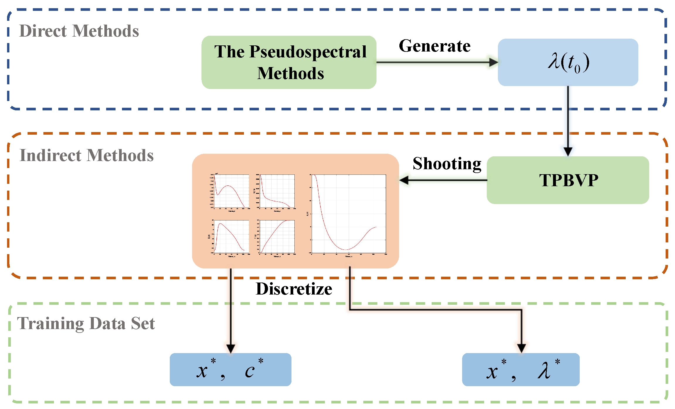However, when high-precision solutions are required, the computational cost increases with the increase in the number of discrete variables, and the direct method cannot guarantee the first order necessary condition [13,14,15,16,17,18]. Based on the calculus of variations and Pontryagin’s minimum principle, the indirect method converts the OCP into a two-point boundary value problem (TPBVP) [19]. The shooting methods can solve this TPBVP by guessing the initial costate and correcting it to obtain the optimal solution. The most attractive advantage of the indirect method is that it guarantees the local optimality of the solution from the theoretical level through the first-order necessity condition, and finally obtains a high-fidelity solution. However, the convergence range of the indirect method is very small and it can hardly deal with inequality constraints. Additionally, due to the lack of physical meaning, it is difficult to provide sufficiently accurate initial costate variables for the shooting method. An inaccurate initial costate makes the calculation time and the number of iterations greatly increase. Therefore, the real-time performance and stability are difficult to guarantee, which also hampers its onboard application [20,21,22].

In recent years, in the aim of solving problems such as the high computational cost and small convergence region faced by traditional methods, researchers have proposed many methods based on artificial intelligence and machine learning to improve the performance of a trajectory optimization algorithm from different aspects. Izzo fitted the state and control commands at each moment through DNN, and then generated the optimal control model and realized the precise landing of the controlled object in real time [23,24]. Cheng and Wang used DNN to map the initial state and the costate variables, which guarantees the efficiency and success rate of the indirect methods and greatly improves the real-time performance and stability of an onboard trajectory optimization algorithm for spacecraft missions [25,26]. Biggs trained DNN using the pulse engine switching time for spacecraft, improved the trajectory accuracy of Bang-Bang control, and ensured the validity of a depth neural network using in discrete decision-making OCPs [27]. In [28], a deep neural network was combined with a traditional feedback control algorithm to ensure the reliability of a moon landing mission. Because DNN only takes limited simple vector/matrix multiplications [29], the practice of treating DNN as the optimal control predictor greatly improves the real-time performance of onboard trajectory optimization algorithms. Additionally, to solve optimal reconfiguration, some scholars have introduced the neural network into the field of model predictive control and achieved good performance. In [30], in the aim of solving the challenging problem of deep space spacecraft formation flight, the author proposed a new nonlinear adaptive neural control method. In [31], Zhou incorporated neural network into the adaptive formation reconfiguration control scheme to improve the control accuracy while making the system robust to uncertain disturbances. For the nearly optimal reconfiguration and maintenance of a distributed formation flying spacecraft, Silvestrini, S. used a model-based reinforcement learning method and introduced inverse reinforcement learning and long short-term memory network into it. The simulation results showed that the proposed algorithm achieved good performance and solved the reconfiguration scenario, which are challenging tasks for traditional algorithms [32,33]. However, the deep neural network is a black box model and is not interpretable, so the safety of a trajectory optimization algorithm cannot be demonstrated [34].

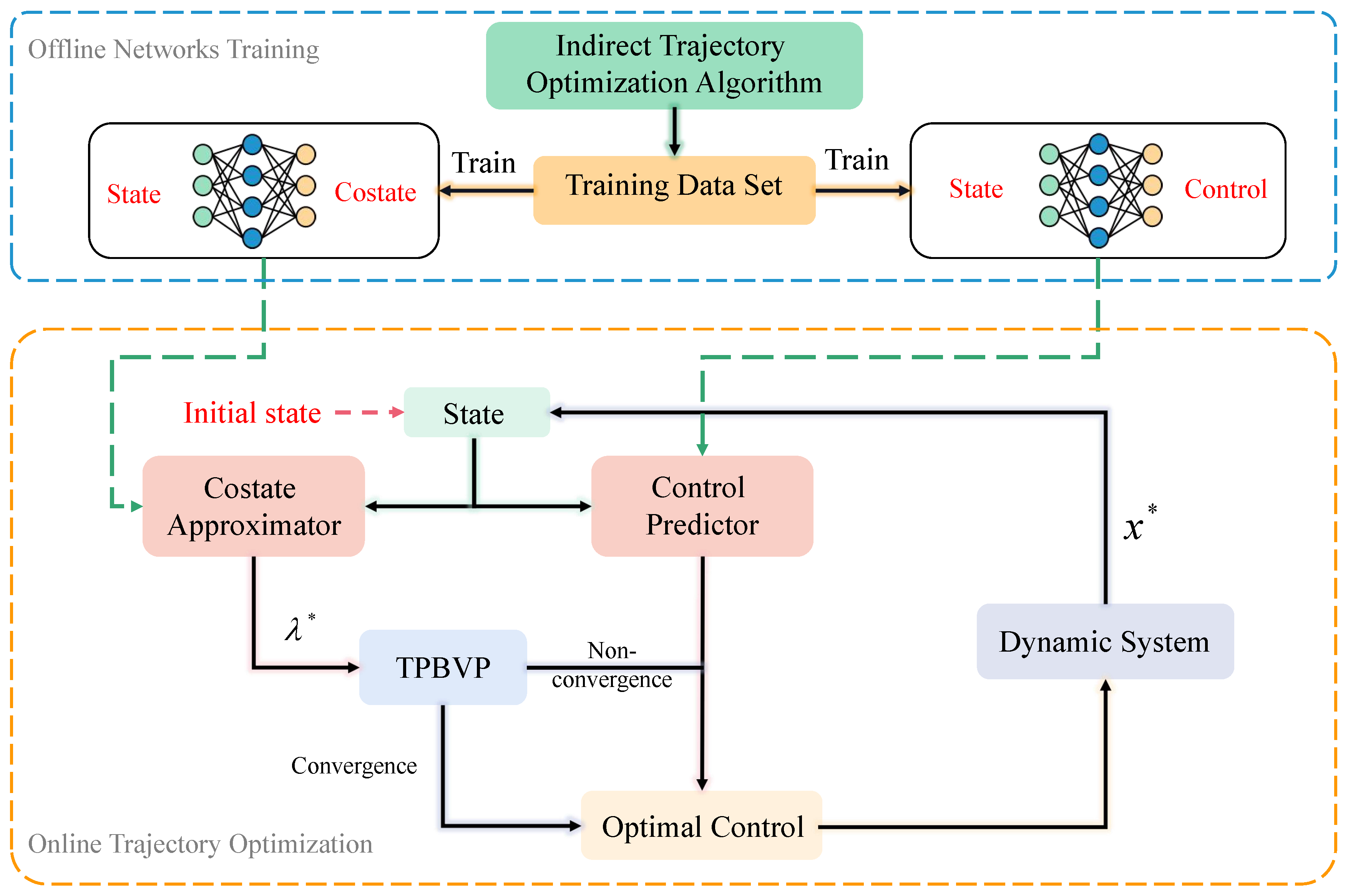
A traditional trajectory optimization algorithm is confronted with difficulties in onboard application due to time-consuming computational requirements, while the direct use of the neural networks as controllers may lead to a lack of reliability in a trajectory optimization algorithm. To solve this problem, in this paper, optimal control theory was tightly combined with a neural network to build a real-time and stable trajectory optimization algorithm with a certain level of intelligence. Specifically, the contributions of this paper are as follows: first, a neural network-based warm-started indirect trajectory optimization method is proposed to ensure its onboard application. The initial costate variables obtained from the well-trained neural network can warm-start the indirect method’s shooting. Second, in order to further ensure the security and stability of the algorithm, the neural network-based optimal action predictor is designed by mapping the nonlinear functional relationship between the state and the optimal action. Then, a backup optimal control variables generation strategy is provided in the case of indirect method shooting failure. Third, two typical spacecraft flight missions are used to verify the feasibility and versatility of the proposed algorithm.

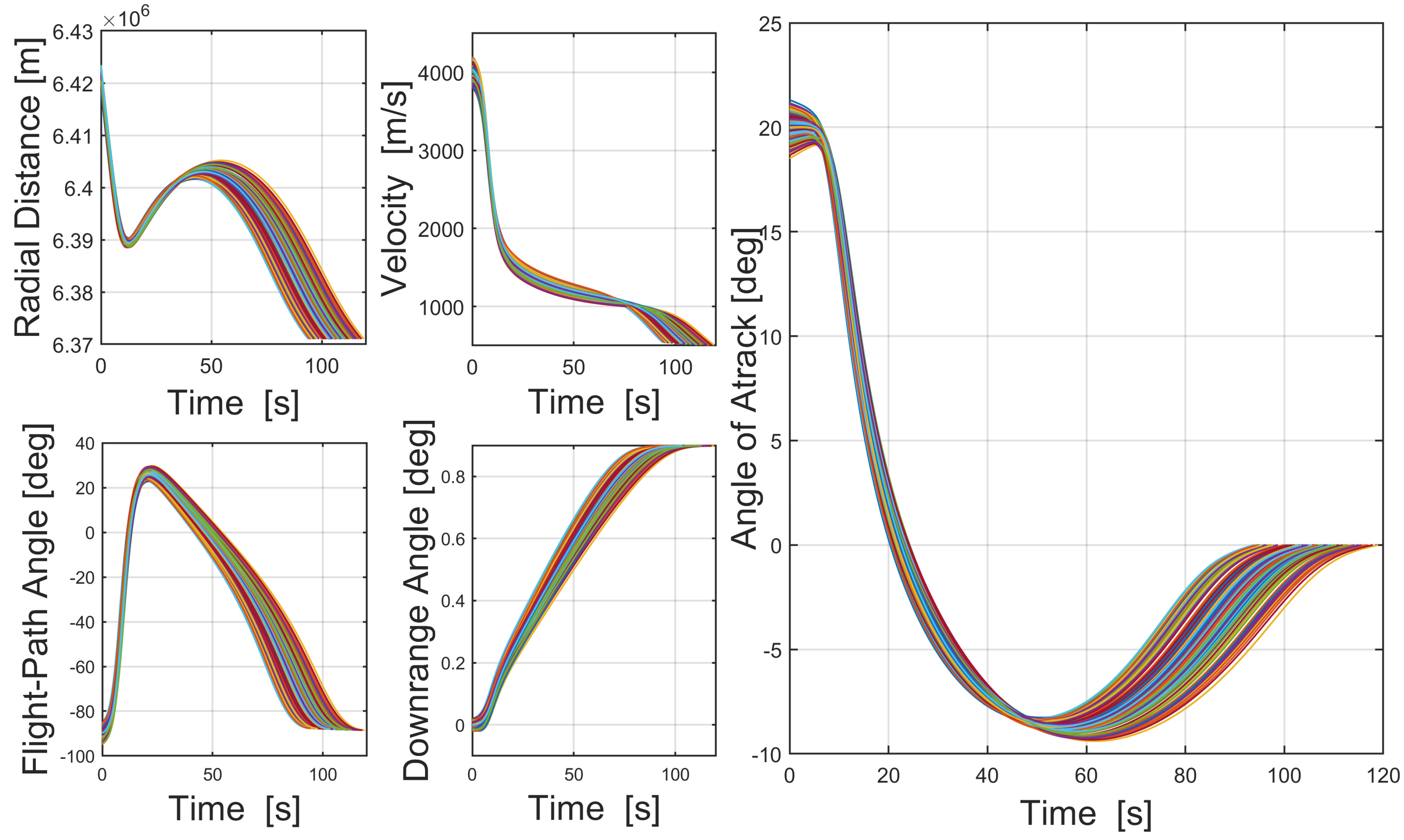
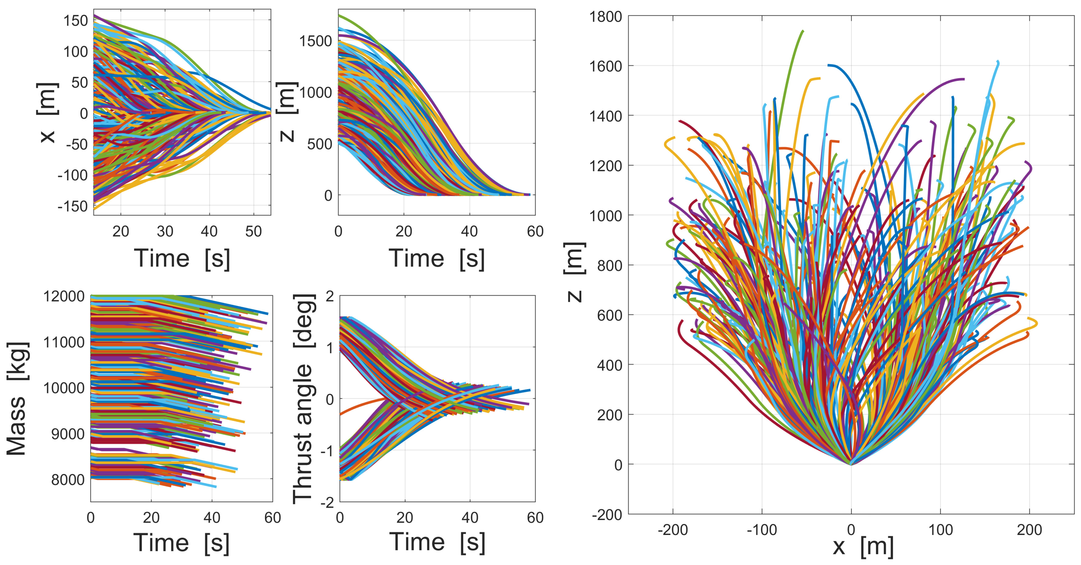
The organization structure of this paper is as follows: Section 2 presents the formulation of the hypersonic vehicle reentry (HVR) problem and fuel-optimal moon landing (FOML) problem. Then, based on Pontryagin’s minimize principle, the formulation of TPBVP and the optimal condition are derived in Section 3, and the generation of training dataset is discussed. In Section 4, the DNNs are trained and the proposed trajectory optimization method is presented. In Section 5, the performance of the proposed method is verified by numerical simulations. Relevant work is summarized in Section 6.

2. Problem Formulation

In this paper, two typical space vehicles with the requirements of high autonomy and optimality are studied, which are hypersonic reentry vehicles and lunar landing vehicles. This section presents the formulations of system dynamics for two different OCPs. The establishment of a physical model and formula derivation meet the following assumptions:

Assumption 1.

Because the motion time of spacecraft is very short relative to a planet day, the planet rotation and its Coriolis effect are ignored;

Assumption 2.

Spacecraft can be treated as a point mass to ignore their own attitude.

2.1. Trajectory Optimization of Hypersonic Reentry

Based on Assumptions 1 and 2, the two-dimensional (2D) unpowered flight equation of motion for a hypersonic vehicle can be expressed as:

$$\left\{\begin{array}{c}\frac{dr}{dt}=vsin\gamma \hfill \\ \frac{dv}{dt}=-\frac{D}{m}-\frac{\mu sin\gamma }{r^2}\hfill \\ \frac{d\gamma }{dt}=\frac{L}{mv}+(\frac{v}{r}-\frac{\mu }{v{r}^2})cos\gamma \hfill \\ \frac{d\theta }{dt}=\frac{vcos\gamma }{r}\hfill \end{array}\right.$$

(1)

where r is the radial distance from a hypersonic vehicle to the center of the Earth, v and m represent the speed and mass of the spacecraft, respectively, $\gamma$ and $\theta$ represent the flight-path angle and downrange angle. The gravitational constant is denoted as $\mu$. The drag and lift D and L are defined by:

$$\begin{array}{cc}\hfill & D=0.5\rho S{C}_D{v}^2\hfill \\ \hfill & L=0.5\rho S{C}_L{v}^2\hfill \end{array}$$

(2)

where S is the reference area, $\rho$ is the calculation of the Earth’s atmospheric density using Boltzmann approximation formula, $C_D$ and $C_L$ are aerodynamic lift and drag coefficients, respectively. $\rho$ is a function of radial distance r, while $C_D$ and $C_L$ can be defined as a function of control variables $\alpha$ which are the angle of attack

$$\begin{array}{cc}\hfill & C_D=1.6537{\alpha }^2+0.0612\hfill \\ \hfill & C_L=1.5658\alpha \hfill \\ \hfill & \rho ={\rho }_{0}exp((r_0-r)/h_S)\hfill \end{array}$$

(3)

where $r_0$ is the initial radial distance, ${\rho }_0$ and $h_S$ are both constants.

Constrained by the initial state and some final states, the performance index of a hypersonic vehicle is to maximize the terminal landing speed. Then, the 2D optimal control problem for the hypersonic vehicle can be written as

$$\begin{array}{c}J=\underset{\alpha }{\min }-v{\left(t_f\right)}^2\\ \mathrm{s}.\mathrm{t}.\dot{\mathit{x}}=f(\mathit{x},\alpha )\\ r\left(t_0\right)=r_0,v\left(t_0\right)=v_0,\\ \gamma \left(t_0\right)={\gamma }_0,\theta \left(t_0\right)={\theta }_0\end{array}$$

(4)

where $\mathit{x}={[r,v,\gamma ,\theta ]}^T$ denotes the state vector, and $\dot{\mathit{x}}=f(\mathit{x},\alpha )$ denotes the system dynamics equation.

2.2. Trajectory Optimization of Fuel-Optimal Moon Landing

In fuel-optimal moon landing guidance, the spacecraft will descend and finally land on a target point at near-zero speed. The Cartesian coordinate system is established with the target point as the origin. Then, the 2-D dynamical equation of the spacecraft can be written as

$$\left\{\begin{array}{c}\frac{d\mathit{r}}{dt}=\mathit{v}\hfill \\ \frac{d\mathit{v}}{dt}=\frac{{\mathit{T}}_{\mathit{c}}}{m}+\mathit{g}\hfill \\ \frac{dm}{dt}=-\frac{T}{I_{sp}{g}_e}\hfill \end{array}\right.$$

(5)

where $\mathit{r}=[x,z]$ denotes the spacecraft’s position, m denotes the spacecraft’s mass, $\mathit{v}=[v_x,v_z]$ is its two-dimensional velocity vector, ${\mathit{T}}_{\mathit{c}}=[Tsin\theta ,Tcos\theta ]$ is its thrust vector, $T\in [0,T_{max}]$ is the magnitude of thrust, and $\theta \in [-\pi /2,\pi /2]$ is the thrust angle. $\mathit{g}=[0,-g_m]$ represents the gravitational acceleration vector and $g_m=$ 1.6229 m/s${}^2$. The specific impulse $I_{sp}$ = 311 s denotes the rocket engine efficiency. The constant $g_e=$ 9.81 m/s${}^2$ denotes the Earth’s gravitational acceleration.

Taking the boundary constraint and the performance index into consideration, the fuel-optimal moon landing problem can be formulated as

$$\begin{array}{c}J=\underset{T,\theta }{\min }{\int }_{t_0}^{t_f}\frac{T}{I_{sp}{g}_e}dt\\ \mathrm{s}.\mathrm{t}.\dot{\mathit{x}}=f(\mathit{x},T,\theta )\\ x\left(t_0\right)=x_0,z\left(t_0\right)=z_0\\ v_x\left(t_0\right)=v_{x_0},v_z\left(t_0\right)=v_{z_0}\end{array}$$

(6)

where $\mathit{x}={[x,z,v_x,v_z,m]}^T$ denotes the state vector, $\dot{\mathit{x}}=f(\mathit{x},T,\theta )$ denotes the system dynamics equation.

3. Generation of the Training Dataset

3.1. Formulation of the TPBVPs and Optimal Conditions

3.1.1. Optimal Conditions of the HVR

According to Pontryagin’s minimum principle, the Hamiltonian function associated with the OCP can be formulated as

$$H={\mathbf{\lambda }}^{T}f={\lambda }_r(vsin\gamma )+{\lambda }_v(-\frac{D}{m}-\frac{\mu sin\gamma }{r^2})+{\lambda }_{\gamma }(\frac{L}{mv}+\frac{v}{r}cos\gamma -\frac{\mu }{v{r}^2}cos\gamma )+{\lambda }_{\theta }\left(\frac{vcos\gamma }{r}\right)$$

(7)

where $\mathbf{\lambda }={[{\lambda }_r,{\lambda }_v,{\lambda }_{\gamma },{\lambda }_{\theta }]}^T$ is the costate vector and ${\lambda }_r,{\lambda }_v,{\lambda }_{\gamma },{\lambda }_{\theta }$ are the costate variables for $r,v,\gamma ,\theta ,$ respectively. Then, with the necessary conditions of optimality, the optimal control variable ${\alpha }^{*}$ can be calculated from the formula $\frac{\partial H}{\partial \alpha }=0$ as follows

$${\alpha }^{*}=\frac{1.5658{\lambda }_{\gamma }}{3.3074v{\lambda }_v}.$$

(8)

Additionally, from $\dot{\mathbf{\lambda }}=-\frac{\partial H}{\partial \mathbf{x}}$, we can obtain the Euler–Lagrange equation of ${\lambda }_r,{\lambda }_v,{\lambda }_{\gamma },{\lambda }_{\theta }$ as follows:

$$\left\{\begin{array}{c}{\dot{\lambda }}_r=-\frac{\partial H}{\partial r}=\left(\frac{vcos\gamma }{r^2}\right){\lambda }_{\theta }-(\frac{D}{h_S}+\frac{2\mu sin\gamma }{r^3}){\lambda }_v+(\frac{L}{h_{S}v}+\frac{vcos\gamma }{r^2}-\frac{2\mu cos\gamma }{v{r}^3}){\lambda }_{\gamma }\hfill \\ {\dot{\lambda }}_v=-\frac{\partial H}{\partial v}=-(sin\gamma ){\lambda }_v-\left(\frac{cos\gamma }{r}\right){\lambda }_{\theta }+\left(\frac{2D}{v}\right){\lambda }_{\gamma }-(\frac{L}{v^2}+\frac{cos\gamma }{r}+\frac{\mu cos\gamma }{v^2{r}^2}){\lambda }_{\gamma }\hfill \\ {\dot{\lambda }}_{\gamma }=-\frac{\partial H}{\partial \gamma }=-(vcos\gamma ){\lambda }_r+\left(\frac{vsin\gamma }{r}\right){\lambda }_{\theta }+\left(\frac{\mu cos\gamma }{r^2}\right){\lambda }_v+(\frac{vsin\gamma }{r}-\frac{\mu sin\gamma }{v{r}^2}){\lambda }_{\gamma }\hfill \\ {\dot{\lambda }}_{\theta }=-\frac{\partial H}{\partial \theta }=0.\hfill \end{array}\right.$$

(9)

The state equation and the costate equation constitute the basic control equations of the indirect method for trajectory optimization. Additionally, according to the transversal conditions, because of the terminal state constraints, we can obtain the terminal costate by formula

$${\mathbf{\lambda }}^{*}\left({t_f}^{*}\right)={\left.(\frac{\partial \phi }{\partial \mathit{x}}+\frac{\partial {\mathit{N}}^T}{\partial \mathit{x}}\mathit{c})\right|}_{t={t_f}^{*}}.$$

(10)

According to the terminal cost function and the boundary conditions

$$\begin{array}{c}\phi =v{\left(t_f\right)}^2\\ \mathit{N}=[r\left(t_f\right)-r_f,\theta \left(t_f\right)-{\theta }_f].\end{array}$$

(11)

Due to $\mathit{c}$ being the unknown parameter, the nontrivial transversality condition can be obtained as follows

$$\begin{array}{c}{\lambda }_v\left(t_f\right)=-2v\left(t_f\right)\\ {\lambda }_{\gamma }\left(t_f\right)=0.\end{array}$$

(12)

Since the Hamiltonian function, terminal cost function and boundary conditions do not explicitly contain $t_f$ and the terminal time is free, the terminal time $t_f$ can be obtained by the following formula

$$H({\mathit{x}}^{*},{\alpha }^{*},t_f)=0.$$

(13)

Finally, the OCP is transformed into TPBVP containing system dynamics as Equation (1), the Euler–Lagrange equation as Equation (9), boundary conditions as Equation (4) and the transversality condition as Equation (11). By integrating an appropriate initial value and correcting it with residuals, the numerical solution of TPBVP can be solved by shooting method [35]. The corresponding shooting function for the unpowered flight of a hypersonic vehicle is

$$\Phi \left(\mathit{Z}\right)=[r\left(t_f\right)-r_f,\theta \left(t_f\right)-{\theta }_f,{\lambda }_v\left(t_f\right)+2v\left(t_f\right),{\lambda }_{\gamma }\left(t_f\right),H\left(t_f\right)]=\mathbf{0}.$$

(14)

where the shooting vector is $\mathit{Z}=[{\lambda }_r\left(t_0\right),{\lambda }_v\left(t_0\right),{\lambda }_{\gamma }\left(t_0\right),{\lambda }_{\theta }\left(t_0\right),t_f]$, see the

Table 1. The parameters for the unpowered flight of the hypersonic vehicle.

Parameter	Value	Unit
m	100	kg
S	0.3	m${}^2$
${\rho }_0$	1.29	-
$h_S$	8.7388 $\times {10}^3$	-
$r_f$	6.371 $\times {10}^3$	m
${\theta }_f$	0.8983	deg

for relevant parameters, initial state and final state.

3.1.2. Optimal Conditions of FOML

For the fuel-optimal moon landing problem formulated in Equation (6), the Hamiltonian function associated with the OCP can be written as

$$H={\mathbf{\lambda }}^{T}f+\frac{T}{I_{sp}{g}_e}={\mathbf{\lambda }}_{\mathit{r}}\mathit{v}+{\mathbf{\lambda }}_{\mathit{v}}(\frac{{\mathit{T}}_{\mathit{c}}}{m}+\mathit{g})-{\lambda }_m\left(\frac{T}{I_{sp}{g}_e}\right)+\frac{T}{I_{sp}{g}_e}$$

(15)

where $\mathbf{\lambda }=[{\lambda }_x,{\lambda }_z,{\lambda }_{v_x},{\lambda }_{v_z},{\lambda }_m]$ is the costate vector and ${\lambda }_x,{\lambda }_z,{\lambda }_{v_x},{\lambda }_{v_z},{\lambda }_m$ are the costate variables for $x,z,v_x,v_z,m$, respectively. Then, from the necessary conditions of optimality $\frac{\partial H}{\partial \theta }=0$ and $\frac{\partial H}{\partial T}=0$, the optimal control variable ${\theta }^{*}$ and $T^{*}$ can be derived as follows:

$$\begin{array}{c}[sin{\theta }^{*},cos{\theta }^{*}]=-\frac{{\mathbf{\lambda }}_{\mathit{v}}}{{∥{\mathbf{\lambda }}_{\mathit{v}}∥}_2}\hfill \\ \left\{\begin{array}{c}T=0,\rho >0\hfill \\ T=T_{max},\rho <0\hfill \\ T=[0,T_{max}],\rho =0\hfill \end{array}\right.\hfill \end{array}$$

(16)

in which the switching function can be formulated as

$$\rho =1-\frac{I_{sp}{g}_e{∥{\lambda }_v∥}_2}{m}-{\lambda }_m.$$

(17)

Meanwhile, according to the necessary conditions of costate variables $\dot{\mathbf{\lambda }}=-\frac{\partial H}{\partial \mathbf{x}}$, the Euler–Lagrange equation can be written as

$$\begin{array}{c}{\dot{\lambda }}_r=-\frac{\partial H}{\partial r}=0\hfill \\ {\dot{\lambda }}_v=-\frac{\partial H}{\partial v}=-{\lambda }_r\hfill \\ {\dot{\lambda }}_m=-\frac{\partial H}{\partial m}=-\frac{T{∥{\lambda }_v∥}_2}{m^2}.\hfill \end{array}$$

(18)

Since terminal mass $m_f$ is not constrained, then we can obtain the transversality condition as follows

$$\begin{array}{c}\hfill {\lambda }_m\left(t_f\right)=0.\end{array}$$

(19)

In this fuel-optimal landing problem, the $t_f$ was free, so the terminal time is determined by

$$H({\mathit{x}}^{*},T^{*},{\theta }^{*},t_f)=0.$$

(20)

Eventually, the system dynamics in Equation (5), the Euler–Lagrange Equation (9), boundary conditions Equation (6) and the transversality condition Equation (19) constitute this TPBVP of the fuel-optimal moon landing problem. The corresponding shooting function of the problem can be formulated as

$$\Phi \left(\mathit{Z}\right)=[x\left(t_f\right),z\left(t_f\right),v_x\left(t_f\right),v_z\left(t_f\right),{\lambda }_m\left(t_f\right),H\left(t_f\right)]=\mathbf{0}$$

(21)

where the shooting vector is $\mathit{Z}=[{\lambda }_x\left(t_0\right),{\lambda }_z\left(t_0\right),{\lambda }_{v_x}\left(t_0\right),{\lambda }_{v_z}\left(t_0\right),t_f]$, and the relevant parameters are listed in

Table 2. The parameters for moon landing.

Parameter	Value	Unit
$T_{max}$	44,000	N
$I_{sp}$	311	s
$g_e$	9.81	m/s${}^2$
$g_m$	1.6229	m/s${}^2$

.

3.2. Dataset Generation Strategy

As we know, the indirect method can generate solutions with high fidelity, but the difficulty of guessing a relatively accurate initial costate makes the TPBVPs hard to solve or even use shooting methods. According to the costate mapping theory [36], the Lagrange multipliers obtained from the pseudospectral method can be used to approximate the costate in the indirect method. For the shooting equation in the indirect method, there are very ideal initial guesses [37]. To solve the initial value sensitivity problem of the indirect method, the pseudospectral method is used in this paper to accelerate the convergence of the indirect method’s shooting process. The OCP solver GPOPS-II [16] is based on the principle of a pseudospectral method, which is used in this paper to provide the warm-started initial value for indirect method’s shooting. Additionally, based on Bellman’s principle of optimality, regardless of its initial state and initial action, its subsequent actions must constitute an optimal strategy for the process taking the state formed by the first decision as the initial state [38]. Consequently, the optimal trajectories can be discretized to state–costate sample pairs and state–action sample pairs for DNNs to learn the nonlinear functional relation.

The generation process of the training dataset is shown in Figure 1. First, the trajectory optimization problem is solved by the pseudospectral method. Then, TPBVP will be derived from OCP. Based on the costate mapping theory, the Lagrange multipliers obtained from the pseudospectral method are considered as initial costate variables $\mathbf{\lambda }\left(t_0\right)$ to work out the TPBVP and generate the single optimal trajectory. Finally, the optimal trajectories will be discretized and divided into two datasets to train two DNN models for each optimal control problem, respectively. For each problem, the symbols in Figure 1 have different meanings. See

Table 3. Symbolic meaning of two OCPs.

Optimal Control Problem	Symbol	Meaning
Hypersonic Vehicle Reentry	$\lambda \left(t_0\right)$	$[{\lambda }_r\left(t_0\right),{\lambda }_v\left(t_0\right),{\lambda }_{\gamma }\left(t_0\right),{\lambda }_{\theta }\left(t_0\right)]$
	$x^{*}$	$[r^{*},v^{*},{\gamma }^{*},{\theta }^{*}]$
	$c^{*}$	${\alpha }^{*}$
	${\lambda }^{*}$	$[{{\lambda }_r}^{*},{{\lambda }_v}^{*},{{\lambda }_{\gamma }}^{*},{{\lambda }_{\theta }}^{*}]$
Fuel-Optimal Moon Landing	$\lambda \left(t_0\right)$	$[{\lambda }_x\left(t_0\right),{\lambda }_z\left(t_0\right),{\lambda }_{v_x}\left(t_0\right),{\lambda }_{v_Z}\left(t_0\right),{\lambda }_m\left(t_0\right)]$
	$x^{*}$	$[x^{*},z^{*},{v_x}^{*},{v_Z}^{*},m^{*}]$
	$c^{*}$	$[T^{*},{\theta }^{*}]$
	${\lambda }^{*}$	$[{{\lambda }_x}^{*},{{\lambda }_z}^{*},{{\lambda }_{v_x}}^{*},{{\lambda }_{v_z}}^{*},{{\lambda }_m}^{*}]$

for details.

Traditional trajectory optimization methods usually assume that the initial state of the spacecraft is known, and the time-consuming process of solving an optimal trajectory is required to be calculated offline. In this paper, however, we aimed to propose an intelligent controller that can guide spacecraft from any state to a fixed point. To reach achieve this goal, the trajectory should cover as much state space as possible to ensure that the DNNs fully learn the dynamics system of a spacecraft in different states and improve the autonomous decision-making ability of intelligent controllers.

The initial state spaces of trajectory generation for two different OCPs are shown in

Table 4. The initial state spaces of the trajectory.

Optimal Control Problem	Parameter	Value Range	Unit
Hypersonic Vehicle Reentry	$r_0$	[6.4185 × ${10}^6$, 6.4235 × ${10}^5$]	m
	${\theta }_0$	[−0.02, 0.02]	deg
	$v_0$	[3800, 4200]	m/s
	${\gamma }_0$	[−95, −85]	deg
Fuel-Optimal Moon Landing	$x_0$	[−200, 200]	m
	$z_0$	[500, 2000]	m
	${v_x}_0$	[−10, 10]	m/s
	${v_z}_0$	[−30, 10]	m/s
	$m_0$	[8000, 12,000]	kg

. In this state space, 1000 initial states are randomly generated and used to obtain the optimal trajectories. Then, each trajectory will be discretized into 10,000 points by equal time steps, and finally divided into two datasets according to the training purposes. Additionally, the 10,000,000 optimal sample pairs will be randomly divided into three subsets, a training set, a testing set and a validation set in a ratio of 8:1:1. Figure 2 and Figure 3 show the partial optimal trajectories of the two problems, respectively.

4. Online Trajectory Optimization Method

For each OCP, two neural networks will be trained to ensure the trajectory optimization method’s real-time performance and stability. Using the state–costate samples obtained from the dataset generation strategy, DNN can learn the highly nonlinear relationship between the state vector and the costate vector of the spacecraft optimal control process. Then, the DNN-based costate approximator will be used to warm-start the shooting method and ensure its onboard application. The other DNN-based control predictor will map the relationship between the spacecraft state and optimal control. As an alternative, this model will calculate the optimal control in the case in which the TPBVP shooting fails. The design and training of the neural networks will be discussed after.

4.1. Overall Framework of Proposed Approach

As shown in Figure 4, the overall framework of the proposed neural network warm-started indirect trajectory optimization method (NWITO) mainly includes two stages: the offline training stage and online control stage. Due to the large differences in the values of the state, costate and control variables, the samples obtained will be normalized to obtain a faster convergence speed of the neural network. Then, through offline training, DNN models can approximate costate and predict the optimal control. Shooting for TPBVP is the core of the onboard algorithm frame, while the costate approximator provides the initial costate to ensure the real-time performance of shooting and the control predictor can generate optimal control to guarantee the stability of the overall algorithm. Benefiting from advanced DNN techniques, this approach has a strong capability to overcome the difficulties of initial costate sensitivity and guarantee the security of the onboard trajectory optimization method.

4.2. Design and Training of DNN

In this subsection, the DNNs will be developed in detail. Because of the limited space, we only discuss the network structure and the related parameter selection of the costate approximator for the HVR problem. The other neural network parameter selection is also the same as what will be discussed. Since the outputs are dependent on the current state, the neural networks mentioned in this paper are all feedforward fully connected neural networks.

A good section of the activation function (AF) for a hidden layer and output layer can improve the nonlinear approximate ability of a DNN model. The commonly used AFs are Linear ($-\infty ,+\infty$), ReLU [0, $+\infty$), Sigmoid (0, 1), Tanh (−1, 1), Softplus (0, $+\infty$), etc. Because ReLU can accelerate the training of the model, it is adopted in the hidden layer. Considering that the value of costate has no fixed value range, Linear can be selected as the AF of the output layer. The loss functions are often used as learning criteria for model optimization problems, that is, the model is solved and evaluated by minimizing the loss function. Here, the mean squared error (MSE) and mean absolute error (MAE) are selected as the loss functions for different DNN models which is defined as

$$\begin{array}{cc}\hfill & MSE:L\left(\omega \right)=\frac{1}{N}\sum _{i=1}^N{(Net\left(\left.x_i\right|\omega \right)-y_i)}^2\hfill \\ \hfill & MAE:L\left(\omega \right)=\frac{1}{N}\sum _{i=1}^N\left|Net\left(\left.x_i\right|\omega \right)-y_i\right|.\hfill \end{array}$$

(22)

The structure of a neural network also has a great influence on its nonlinear approximation effect. Excessively complex networks tend to perform well on training sets, but not on testing sets. This is because the network learns non-critical features in the dataset, which is called over-fitting. However, excessively simple neural network models cannot learn the general rules in the dataset due to their insufficient learning ability, which results in weak generalization ability, called under-fitting. Thus, aiming at different datasets, the network structure should be adjusted and find a balance. As we can see in Figure 5, the neural network with three hidden layers is not enough to learn the dynamics relationship of the OCP for the hypersonic vehicle, so its performance in the training set and testing set is not satisfactory. Too many layers and neural units will make the model more complex and fall into the situation of over-fitting. Considering the performance of a neural network in a training set and testing set, the network scale was chosen as 4 layers/64 units.

As shown in Figure 6, loss values were compared by ten-fold cross-validation under different parameters of batch size and learning rate. Then, the batch size is determined as 128 and the learning rate is 0.00001. Additionally, the Adam algorithm [39] is found to be competent for minimizing the loss function as the optimizer in this study.

Table 5. Network structure of the DNNs for two OCPs.

Optimal Control Problem	Neural Network	Activation Function	Size	Loss Function
Hypersonic Vehicle Reentry	Net${}_c$	ReLU	4 Layers / 64 Units	MAE
	Net${}_{\lambda }$	ReLU	4 Layers / 128 Units	MSE
>Fuel-Optimal Moon Landing	Net${}_{u_1}$	ReLU	2 Layers / 14 Units	MAE
	Net${}_{\theta }$	tanh	3 Layers / 14 Units	MSE
	Net${}_{\lambda }$	ReLU	5 Layers / 128 Units	MSE

displays the relevant parameter settings of other neural networks about two OCPs.

Based on the selected parameters, including the activation function, the number of hidden layers, the number of hidden layer units, batch size, learning rate, etc., the neural network can converge to the optimal value, mapping the highly nonlinear relationship of the OCP for spacecraft. Algorithm 1 is the pseudocode implementation to train the neural network.

Algorithm 1 Supervised training algorithm of the DNNs

Input:  $x^{*}$ Output:  ${\lambda }^{*}$, $c^{*}$   1: Normalize training dataset including $[x^{*},{\lambda }^{*}],[x^{*},c^{*}],[x^{*},t^{*}]$.   2: From uniform distribution, randomly initialize $Ne{t}_{\lambda }\left(x\right|{\omega }^{\lambda }),Ne{t}_c\left(x\right|{\omega }^c)$ and $Ne{t}_t\left(x\right|{\omega }^t)$ with weights and bias.   3: for each $epoch\in [1,N]$ do   4:    Randomly select a minibatch of sample from normalized training dataset.   5:    Minimize the loss function and update $Net$ with Adam algorithm.   6: end for

5. Simulation and Results

In this section, numerical simulations are implemented to evaluate the performance of the proposed NWITO algorithm. All the simulations are accomplished on a desktop computer with an Intel Core-i7-11700@2.50GHz CPU, a NVIDIA GeForce GTX 1650 SUPER GPU and 16.0 GB RAM. The training of a neural network and the proposed NWITO algorithm programs are coded based on Python 3.6.3 and Tensorflow 2.1.0, and the data-generated strategy programs are coded based on MATLAB 2020b and GPOPS-II.

5.1. Network Approximation Accuracy

Through the selection of neural network parameters and then training with the state–costate pairs and state–control pairs obtained in the previous section, neural networks are designed as a costate approximator and a control predictor for different OCPs. Three initial states shown in

Table 6. Initial state vectors of three simulation cases.

Optimal Control Problem	Parameter	Case 1	Case 2	Case 3	Unit
Hypersonic Vehicle Reentry	$r_0$	$\mathrm{6,421,884}$	$\mathrm{6,419,455}$	$\mathrm{6,421,203}$	m
	${\theta }_0$	$-0.0160$	$-0.0157$	$0.0113$	deg
	$v_0$	$3871.48$	$3837.22$	$3855.18$	m/s
	${\gamma }_0$	$-87.42$	$-92.53$	$-85.77$	$deg$
Fuel-Optimal Moon Landing	$x_0$	$49.61$	$-191.60$	$-195.53$	m
	$z_0$	$538.18$	$803.42$	$935.13$	m
	${v_x}_0$	$-8.65$	$3.34$	$-2.66$	m/s
	${v_z}_0$	$-21.68$	$-14.33$	$-9.19$	m/s
	$m_0$	$\mathrm{11,221.17}$	$\mathrm{11,765.67}$	$\mathrm{11,954.65}$	kg

are randomly selected to compare the results of a well-trained costate approximator and the control predictor with the nominal trajectory obtained by the indirect method, and the approximation accuracy is evaluated. As shown in Figure 7 and Figure 8, the black dashed lines are the standard trajectories produced by the indirect method. Based on the corresponding optimal state profiles, DNNs generate costate and control profiles to compare with standard trajectories. Experiments show that the costate approximator and control predictor can learn the highly nonlinear characteristics of the dynamics system and achieve a good fit.

Pearson’s correlation coefficient is a commonly used linear correlation coefficient with values between −1 and 1, which is calculated as follows and is widely used to measure the degree of correlation between two variables [40]. Here, the correlation coefficient is used to conduct the regression analysis of neural networks to qualitatively estimate the approximate accuracy of the network. Figure 9 and Figure 10 show the regression analysis results between the predicted neural network and the target for the two OCPs, respectively. Regression results show that the prediction and target are highly correlated, and the obtained network has a high approximate accuracy for costate and control variables.

$${\rho }_{X,Y}=\frac{cov(X,Y)}{{\sigma }_X,{\sigma }_Y}=\frac{{\sum }_{i=1}^n(X_i-\overline{X})(Y_i-\overline{Y})}{\sqrt{{\sum }_{i=1}^n{(X_i-\overline{X})}^2}\sqrt{{\sum }_{i=1}^n{(Y_i-\overline{Y})}^2}}$$

(23)

5.2. The Performance of the Real-Time Trajectory Optimization Algorithm

In order to verify the optimization of the algorithm, Monte Carlo sampling was used to extract the initial state vector from the state space for the spacecraft’s closed-loop guidance. The state variables of the spacecraft are randomly initialized. Then, the real-time closed-loop guidance is performed using the well-trained intelligent controller described above. For two OCPs, the comparison of the closed-loop guidance trajectory generated by the proposed algorithm with that generated by the indirect method is shown in Figure 11 and Figure 12, respectively. In both cases, the trajectories generated by the proposed algorithm basically overlap the nominal trajectories obtained by the indirect method. Therefore, the designed intelligent controller can learn the nonlinear dynamics characteristics of different spacecraft on the one hand, and on the other hand, it can generate optimal control decisions at each time to drive the spacecraft to achieve the optimal flight satisfying the performance index. In addition, the traditional integration process may eventually result in the non-convergence of flight trajectories due to accumulated errors, while the decision generation by the proposed NWITO method mainly depends on the state variables at the current time. Thus, the trajectory can be corrected in subsequent decisions to drive the spacecraft to achieve a high-precision landing when a low-precision decision occurs at some time.

In order to further analyze the closed-loop guidance effect and generalization ability of the intelligence controller, the Monte Carlo method is used to verify the proposed method. In the numerical simulation, the 1000 initial state vector are randomly generated within the state space range and then the proposed NWITO method is used for closed-loop guidance to the end point, and its maximum terminal error with the nominal trajectory solved by indirect method is calculated and shown in

Table 7. Terminal errors of two OCPs.

Optimal Control Problem	Parameter	Error Range	Unit
Hypersonic Vehicle Reentry	v	$[-0.56,0.35]$	m/s
	r	$[-139,53]$	m
Fuel-Optimal Moon Landing	x	$[-0.2,0.2]$	m
	z	$[-0.16,0.14]$	m
	$v_x$	$[-0.18,0.18]$	m/s
	$v_z$	$[-0.15,0.16]$	m/s
	m	$[-29,-15]$	kg

. The simulation results show that the NWITO method can drive the controlled object to achieve optimal control with high accuracy, and the controller has certain universality and generalization performance.

Because the indirect method has the requirement of integrating several times and shooting to iteratively correct the initial costate estimation, the solving process takes a lot of time and becomes a key factor to limit the online application of a trajectory optimization algorithm. This paper provides a high-precision initial costate mapping model to warm-start TPBVP shooting based on the well-trained neural network. Because the DNN only involves limited simple vector/matrix multiplications, the mapping speed of the network is fast enough to guarantee its online applications. Figure 13 shows the cpu time distribution to solve 1000 trajectories using the indirect method and the proposed method for two OCPs, respectively. The results show that the optimal trajectory generation efficiency of the proposed method is nearly 20 times higher than that of the indirect method. In the HVR problem, the trajectory of 105 s can be solved in only 5 s by the proposed method. In the moon landing problem, the trajectory of 35 s can be obtained in approximately 2 s. It can be concluded that the proposed method can completely meet the requirement of the real-time trajectory generation of spacecraft. The update frequency of the trajectory is adjusted by the time consumed to solve the optimal trajectory, and the simulation results show that the update frequency meets the accuracy requirements. Additionally, the proposed method is based on the TensorFlow framework with Python. Since C is more efficient than Python, it is predicted that if the neural network model under Python is rewritten in C language, the calculation speed of the intelligent trajectory optimization method will be further improved.

6. Conclusions

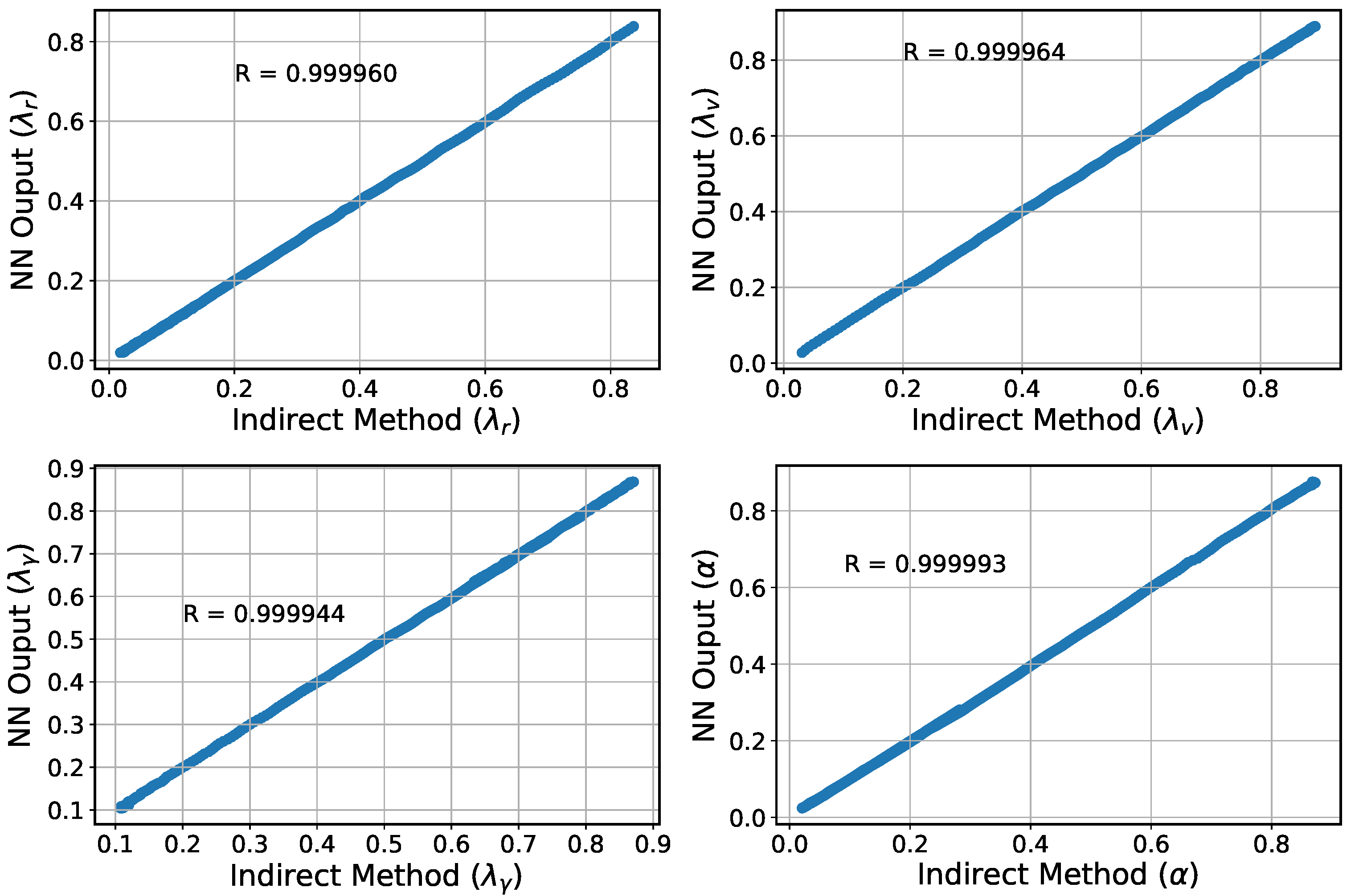
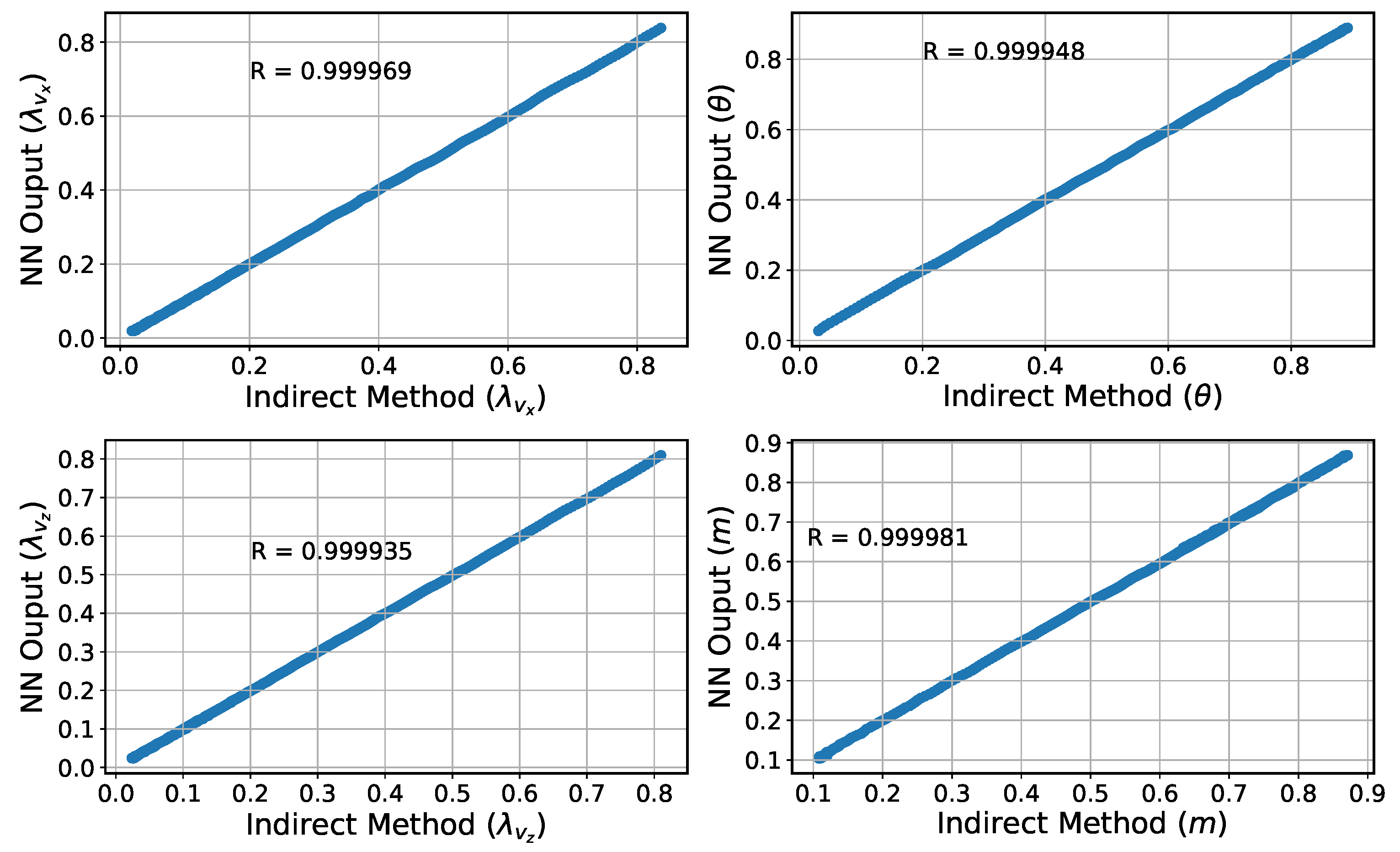
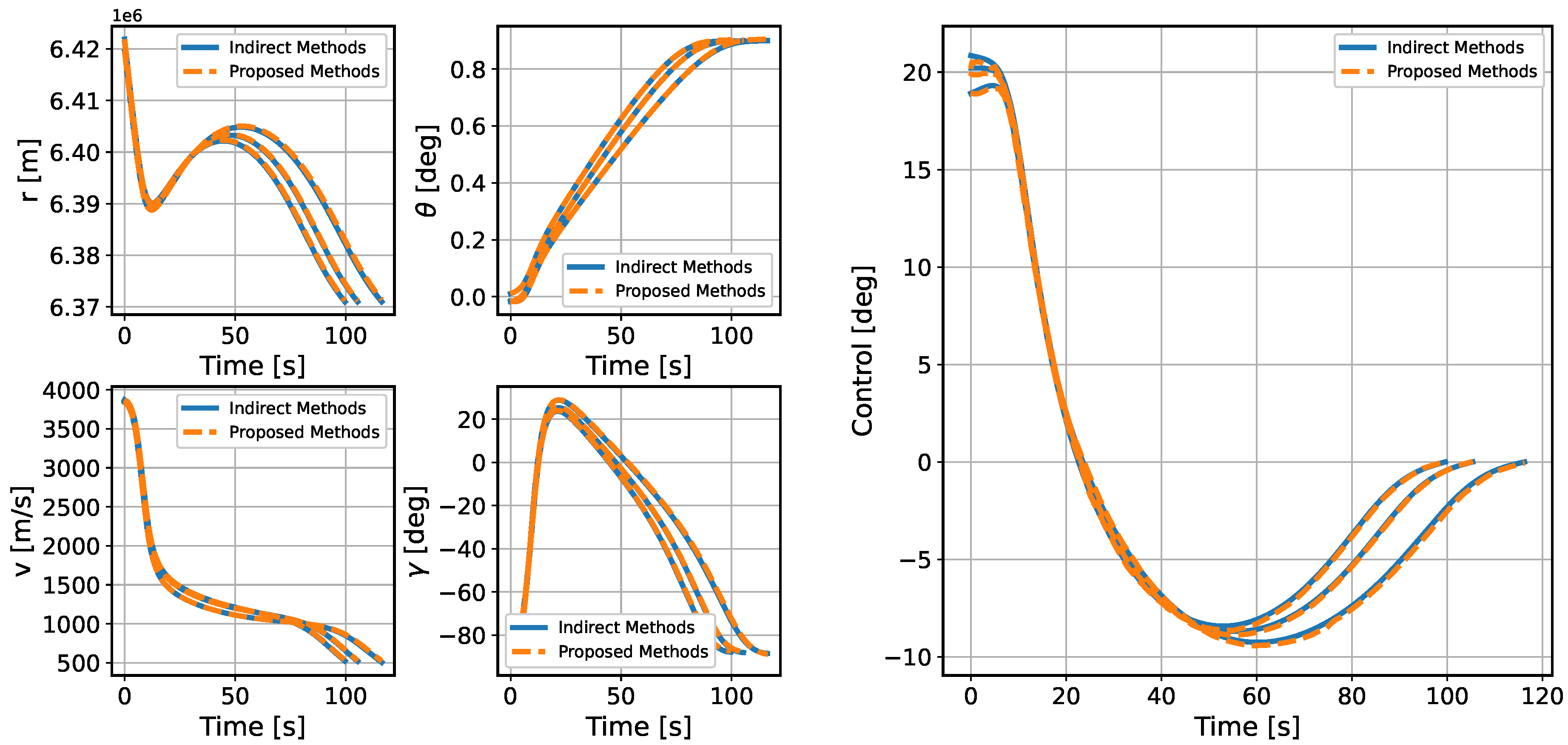
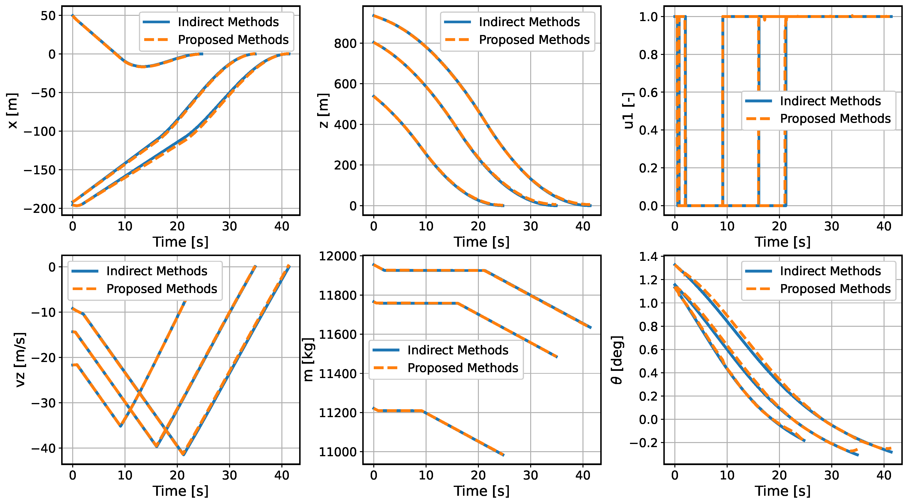
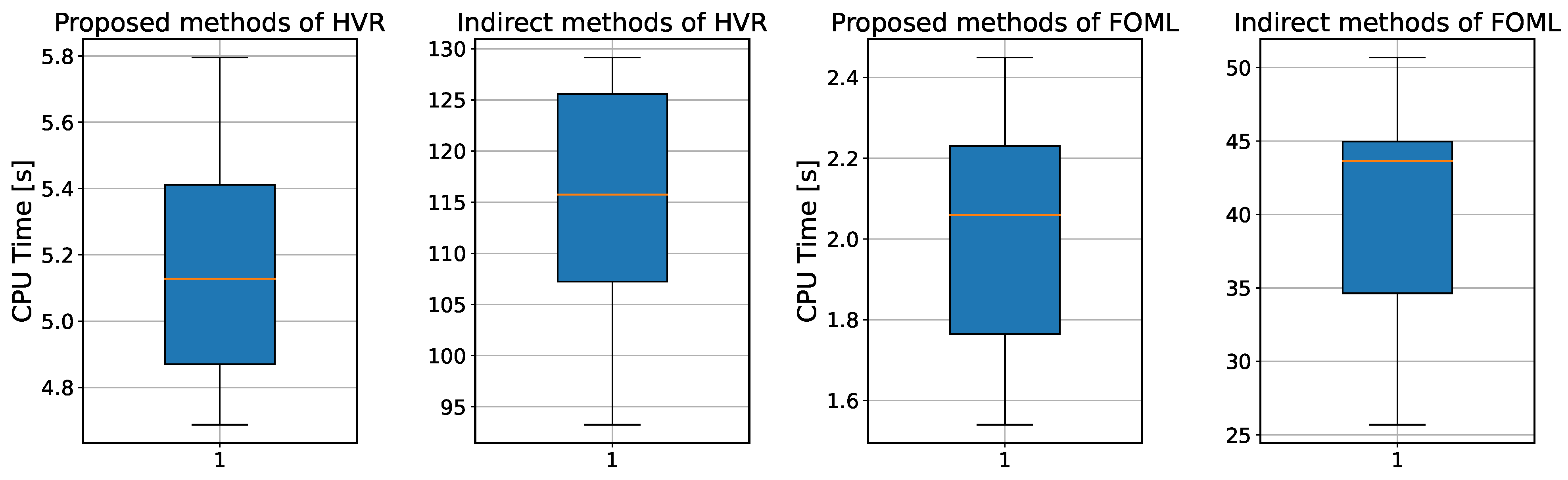
To improve the autonomous decision-making ability and intelligence level of the onboard trajectory optimization algorithm, this paper combines optimal control theory with deep learning method and develops a neural network warm-started indirect trajectory optimization method. First, two typical complex spacecraft flight missions are formulated as OCPs and the corresponding TPBVPs are derived. The pseudospectral method and the shooting method are combined to obtain a high fidelity solution for DNN training. Based on the well-trained DNN model, the proposed method achieves fast solutions to the trajectory optimization problems. Numerical simulations demonstrate that the neural network can learn the highly nonlinear relationship among the variables, and the proposed method has the advantages of good real-time performance, excellent convergence and generalization ability.

In the proposed method, the main strategy can approximate the costate, warm-start the indirect method’s shooting and then drive the spacecraft to achieve optimal control in real time. Furthermore, a backup strategy can further improve the security of onboard algorithms. The method of integrating advanced artificial intelligence algorithms into the traditional optimal control theory provides a novel idea for solving the OCP. Future research considers introducing more complex constraints to the dynamics model to verify the effectiveness of the proposed method. In addition, a nondimensionalized method and backward integration method can be used to accelerate the generation of a training dataset, and more elaborate network structures can be adopted to enhance the accuracy of the algorithm.

References

1. Malyuta, D.; Yu, Y.; Elango, P.; Açıkmeşe, B. Advances in trajectory optimization for space vehicle control. Annu. Rev. Control 2021, 52, 282–315. [Google Scholar] [CrossRef]
2. Chai, R.; Tsourdos, A.; Savvaris, A.; Chai, S.; Xia, Y.; Chen, C.P. Review of advanced guidance and control algorithms for space/aerospace vehicles. Prog. Aerosp. Sci. 2021, 122, 100696. [Google Scholar] [CrossRef]
3. Li, S.; Jiang, X. RBF neural network based secondorder sliding mode guidance for Mars entry under uncertainties. Aerosp. Sci. Technol. 2015, 43, 226–235. [Google Scholar] [CrossRef]
4. Li, S.; Peng, Y. Neural network-based sliding mode variable structure control for Mars entry. J. Aerosp. Eng. 2012, 226, 1373–1386. [Google Scholar] [CrossRef]
5. Bird, J.; Petzold, L.; Lubin, P.; Deacon, J. Advances in deep space exploration via simulators & deep learning. New Astron. 2021, 84, 101517. [Google Scholar]
6. Li, S.; Jiang, X. Review and prospect of guidance and control for Mars atmospheric entry. Prog. Aerosp. Sci. 2014, 69, 40–57. [Google Scholar] [CrossRef]
7. Li, S.; Peng, Y. Command generator tracker based direct model reference adaptive tracking guidance for Mars atmospheric entry. Adv. Space Res. 2012, 49, 49–63. [Google Scholar] [CrossRef]
8. Izzo, D.; Märtens, M.; Pan, B. A survey on artificial intelligence trends in spacecraft guidance dynamics and control. Astrodynamics 2019, 3, 287–299. [Google Scholar] [CrossRef]
9. Betts, J.T. Survey of numerical methods for trajectory optimization. J. Guid. Control Dyn. 1998, 21, 193–207. [Google Scholar] [CrossRef]
10. Gill, P.E.; Murray, W.; Saunders, M.A. SNOPT: An SQP algorithm for large-scale constrained optimization. SIAM Rev. 2005, 47, 99–131. [Google Scholar] [CrossRef]
11. Biegler, L.T.; Zavala, V.M. Large-scale nonlinear programming using IPOPT: An integrating framework for enterprise-wide dynamic optimization. Comput. Chem. Eng. 2009, 33, 575–582. [Google Scholar] [CrossRef]
12. Cheng, L.; Zhang, Q.; Jiang, F. Multi-constrained compound reentry guidance based on onboard model identification. J. Tsinghua Univ. (Sci. Technol.) 2019, 59, 712–719. [Google Scholar]
13. Wall, B.J.; Conway, B.A. Shape-Based Approach to Low-Thrust Rendezvous Trajectory Design. J. Guid. Control Dyn. 2009, 32, 95–101. [Google Scholar] [CrossRef]
14. Subbarao, K.; Shippey, B.M. Hybrid Genetic Algorithm Collocation Method for Trajectory Optimization. J. Guid. Control Dyn. 2009, 32, 1396–1403. [Google Scholar] [CrossRef]
15. Yang, S.; Cui, T.; Hao, X.; Yu, D. Trajectory optimization for a ramjet-powered vehicle in ascent phase via the Gauss pseudospectral method. Aerosp. Sci. Technol. 2017, 67, 88–95. [Google Scholar] [CrossRef]
16. Patterson, M.A.; Rao, A.V. GPOPS-II: A MATLAB Software for Solving Multiple-Phase Optimal Control Problems Using hpAdaptive Gaussian Quadrature Collocation Methods and Sparse Nonlinear Programming. ACM Trans. Math. Softw. 2010, 41, 1–37. [Google Scholar] [CrossRef] [Green Version]
17. Lekkas, A.M.; Roald, A.L.; Breivik, M. Online Path Planning for Surface Vehicles Exposed to UnknownOcean Currents Using Pseudospectral Optimal Control. IFAC-Pap. OnLine 2016, 49, 1–7. [Google Scholar] [CrossRef]
18. Bittner, M.; Fisch, F.; Holzapfel, F. A Multi-Model Gauss Pseudospectral Optimization Method for Aircraft Trajectories. In Proceedings of the AIAA Atmospheric Flight Mechanics Conference, Minneapolis, MN, USA, 13–16 August 2012; p. 4728. [Google Scholar]
19. Hull, D.G. Optimal Control Theory for Applications; Springer: New York, NY, USA, 2013. [Google Scholar]
20. Mansell, J.R.; Grant, M.J. Adaptive Continuation Strategy for Indirect Hypersonic Trajectory Optimization. J. Spacecr. Rocket. 2018, 55, 818–828. [Google Scholar] [CrossRef]
21. Grant, M.J.; Braun, R.D. Rapid Indirect Trajectory Optimization for Conceptual Design of Hypersonic Missions. J. Spacecr. Rocket. 2015, 52, 177–182. [Google Scholar] [CrossRef]
22. Tang, G.; Jiang, F.; Li, J. Fuel-Optimal Low-Thrust Trajectory Optimization Using Indirect Method and Successive Convex Programming. IEEE Trans. Aerosp. Electron. Syst. 2018, 54, 2053–2066. [Google Scholar] [CrossRef]
23. Sánchez-Sánchez, C.; Izzo, D.; Hennes, D. Learning the Optimal State-Feedback Using Deep Networks. In Proceedings of the 2016 IEEE Symposium Series on Computational Intelligence, Athens, Greece, 6–9 December 2016; pp. 1–8. [Google Scholar]
24. Sánchez-Sánchez, C.; Izzo, D. Real-time Optimal Control via Deep Neural Networks: Study on Landing Problems. J. Guid. Control Dyn. 2018, 41, 1122–1135. [Google Scholar] [CrossRef] [Green Version]
25. Cheng, L.; Wang, Z.; Jiang, F.; Li, J. Fast Generation of Optimal Asteroid Landing Trajectories Using Deep Neural Networks. IEEE Trans. Aerosp. Electron. Syst. 2020, 56, 2642–2655. [Google Scholar] [CrossRef]
26. Shi, Y.; Wang, Z. Onboard Generation of Optimal Trajectories for Hypersonic Vehicles Using Deep Learning. J. Spacecr. Rocket 2020, 58, 400–414. [Google Scholar] [CrossRef]
27. Biggs, J.D.; Fournier, H. Neural-network-based optimal attitude control using four impulsive thrusters. J. Guid. Control Dyn. 2020, 43, 299–309. [Google Scholar] [CrossRef]
28. Cheng, L.; Wang, Z.; Jiang, F. Real-Time Control for Fuel-Optimal Moon Landing based on an Interactive Deep Reinforcement Learning Algorithm. Astrodynamics 2019, 3, 375–386. [Google Scholar] [CrossRef]
29. You, S.; Wan, C.; Dai, R.; Lu, P.; Rea, J.R. Learning-based Optimal Control for Planetary Entry, Powered Descent and Landing Guidance. In Proceedings of the AIAA Scitech 2020 Forum, Orlando, FL, USA, 6–10 January 2020; p. 849. [Google Scholar]
30. Gurfil, P.; Idan, M.; Kasdin, N.J. Adaptive neural control of deep-space formation flying. J. Guid. Control Dyn. 2003, 26, 491–501. [Google Scholar] [CrossRef]
31. Zhou, N.; Chen, R.; Xia, Y.; Huang, J.; Wen, G. Neural network-based reconfiguration control for spacecraft formation in obstacle environments. Int. J. Robust Nonlinear Control 2018, 28, 2442–2456. [Google Scholar] [CrossRef]
32. Silvestrini, S.; Lavagna, M.R. Spacecraft Formation Relative Trajectories Tdentification for Collision-Free Maneuvers Using Neural-Reconstructed Dynamics. In Proceedings of the AIAA Scitech 2020 Forum, Orlando, FL, USA, 6–10 January 2020; p. 1918. [Google Scholar]
33. Silvestrini, S.; Lavagna, M.R. Neural-based predictive control for safe autonomous spacecraft relative maneuvers. J. Guid. Control Dyn. 2021, 44, 2303–2310. [Google Scholar] [CrossRef]
34. Zhang, Y.; Tiňo, P.; Leonardis, A.; Tang, K. A Survey on Neural Network Interpretability. IEEE Trans. Emerg. Top. Comput. Intell. 2021, 5, 726–742. [Google Scholar] [CrossRef]
35. Osborne, M.R. On shooting methods for boundary value problems. J. Math. Anal. Appl. 1969, 27, 417–433. [Google Scholar] [CrossRef] [Green Version]
36. Garg, D.; Patterson, M.; Hager, W.W.; Rao, A.V.; Benson, D.A.; Huntington, G.T. A unified framework for the numerical solution of optimal control problems using pseudospectral methods. Automatica 1997, 46, 1843–1851. [Google Scholar] [CrossRef]
37. Fahroo, F.; Ross, I.M. Costate Estimation by a Legendre Pseudospectral Method. J. Guid. Control Dyns. 2001, 24, 270–277. [Google Scholar] [CrossRef]
38. Wang, Y.; O’Donoghue, B.; Boyd, S. Approximate dynamic programming via iterated Bellman inequalities. Int. J. Robust Nonlinear Control 2015, 25, 1472–1496. [Google Scholar] [CrossRef] [Green Version]
39. Kingma, D.P.; Ba, J. Adam: A method for stochastic optimization. arXiv 2014, arXiv:1412.6980. [Google Scholar]
40. Ly, A.; Marsman, M.; Wagenmakers, E.J. Analytic posteriors for Pearson’s correlation coefficient. Stat. Neerla 2018, 72, 4–13. [Google Scholar] [CrossRef]
Figure 1. Training dataset generation framework.
Aerospace 09 00435 g001
Figure 2. Training dataset of HVR problem.
Aerospace 09 00435 g002
Figure 3. Training dataset of FOML problem.
Aerospace 09 00435 g003
Figure 4. The proposed neural network-based warm-started indirect trajectory optimization method.
Aerospace 09 00435 g004
Figure 5. Loss comparisons of DNN with different sizes.
Aerospace 09 00435 g005
Figure 6. Loss comparison of DNN with different sizes.
Aerospace 09 00435 g006
Figure 7. Approximate effect of neural network for HVR.
Aerospace 09 00435 g007
Figure 8. Approximate effect of neural network for FOML.
Aerospace 09 00435 g008
Figure 9. The regression analysis results between the predicted and the standard for HVR.
Aerospace 09 00435 g009
Figure 10. The regression analysis results between the predicted and the standard for FOML.
Aerospace 09 00435 g010
Figure 11. The comparison of the closed-loop guidance trajectory for HVR.
Aerospace 09 00435 g011
Figure 12. The comparison of the closed-loop guidance trajectory for FOML.
Aerospace 09 00435 g012
Figure 13. Comparison of the solving efficiency between the proposed method and the indirect method.
Aerospace 09 00435 g013