An Innovative Pose Determination Algorithm for Planetary Rover Onboard Visual Odometry

Abstract

Planetary rovers play a critical role in space exploration missions, where one of the most fundamental algorithms is pose determination. Due to environmental and computational constraints, real-time pose determinations of planetary rovers can only use low-cost techniques, such as visual odometry. In this paper, by employing the angle-based criterion, a novel pose determination algorithm is proposed for visual odometry, which is suitable for any type of central camera. First, the problem is formulated using the Huber kernel function with respect to the angular residuals. Then, an intermediate coordinate system is introduced between the initial estimation and final refinement. In order to avoid being trapped in periodic local minimums, a linear method is used to further align the reference points between the intermediate and camera coordinate systems. Finally, one step refinement is implemented to optimize pose determinations. The theoretical analysis, the synthetic simulations, and the real experiments show that our proposed algorithm can achieve the best accuracies within similar processing times, compared with the most state-of-the-art algorithms, thereby approving the effectiveness of the proposed algorithm used in planetary rover onboard visual odometry.

1. Introduction

Since Lunokhod 1, the first lunar rover, landed on the Moon in 1970, many planetary rovers have been or are being developed to explore the geology of extraterrestrial planets, opening an effective access towards the unknown universe for mankind. During exploration missions, accurate and real-time pose determination is the prerequisite of various tasks, especially in rover operation and 3D map reconstruction [1]. However, due to environmental and computational constraints, accurate pose determination is always challenging for planetary rovers. No prior information can serve as absolute position reference in unknown environments, such as landmark and global navigation satellite system. Moreover, no loop closure can be employed to compensate the drift accumulated over time, limited by the onboard computing and storage capability. Therefore, planetary rovers can only rely on the pose determination derived solely from either an inertial measurement unit (IMU), wheel odometry (WO), or visual odometry (VO) [2]. Among the above techniques, the performance of VO has shown many advantages in both accuracy and robustness, while IMUs suffer most in height divergence, and WOs encounter traction loss on high-slippage terrains. Therefore, VO has become predominant in recent planetary rovers, such as the CNSA Yutu-2 rover [3], NASA Perseverance rover [4], and ESA Rosalind Franklin rover [5].

In robotics, VO is a technique for determining the position and attitude of a robotic vehicle based on 3D-2D feature correspondences extracted from sequential images. As the most common visual textures on the planet surface, point features are widely used for onboard VO in planetary rovers [6]. Without noise, all the 3D points in a determined pose should align with their corresponding 2D projections. However, due to various sources of noises, the 3D points and their 2D projections can never be fully aligned. Therefore, we should find the optimal pose to align them, using some specific criterion.

As the most significant module in VO, pose determinations based on matched 3D-2D points have been studied in numerous literatures in the past decades. In our opinion, all the algorithms can be categorized into four main criteria, which are the algebraic three-point constraints (ATPC)-based criterion, point-to-point distance (PPD)-based criterion, point-to-line distance (PLD)-based criterion, and the angle-based criterion.

The first one is the ATPC based criterion, which can be expressed as unary quartic polynomials derived from the minimal problems with three points [7]. By utilizing this criterion, a pose determination problem is reorganized as multiple minimal problems with two common points, then the Euclidean norm of the ATPC is minimized by solving a seventh order equation [8]. Apparently, these two common points are emphasized far more than the other points, thus the accuracy of pose determination is greatly degraded when these two points are corrupted severely by noises. Therefore, the ATPC based criterion is usually employed during initialization, then the pose is optimized by iterative methods [9].

In order to improve the accuracy in pose determinations, the PPD-based criterion is developed, which is widely used in current VO systems. Using this criterion, the deviations between reference points and their back-projected image points are minimized. One direct method is anisotropic orthogonal Procrustes analysis, where attitude, position, and scale are optimized successively [10]. This algorithm is robust as it can converge from any reasonable initial scale, but it is time-consuming due to its univariate search strategy. The first non-iterative algorithm with linear complexity was proposed in [11], where four virtual control points were introduced to represent all the reference points in a frame. Due to the benefit from the reduced number of control points and the linearized expressions for reference points, the computational efficiency is significantly improved. After obtaining a linear solution, the weights of the four control points are refined using the PPD-based criterion. Subsequently, outlier rejection [12] and covariance leverage [13] are embedded in this control-point system to improve the performance of pose determinations. Unfortunately, these algorithms may result in unstable estimations in less redundant cases, because of ignoring the orthogonality of rotation matrix in calculations.

To overcome the above issue, the PLD-based criterion has been explored. Based on the PLD criterion, the orthogonal deviations between the reference points and the observed projection lines are minimized. In [14], the optimization problem is decoupled and reformulated in an unconstrained form, where the rotation is parameterized as non-unit quaternions. The answers to its multivariate polynomial equation system are solved in a closed form using the Grobner basis (GB) technique and all stationary points are found accordingly. Note that, the sign ambiguity inherent in quaternions should be handled carefully. Therefore, in more recent works [9,15], the Cayley–Gibbs–Rodriguez (CGR) parameterization is adopted instead and a more compact derivation is proposed. Similarly, the GB method is employed to solve the cubic polynomial equation system. In order to avoid singularity, an accurate initial pose should be acquired [9], or a fixed pre-rotation should be applied [15].

Although fairly accurate pose determination is achieved, the distance-based criteria are neither justified nor likely in real applications [16]. It is more reasonable to use the angle-based criterion, where the noise model is applied to original measurements instead of back-projected distances. Since this criterion is rotationally invariant, it can be utilized for any type of central camera, such as perspective [17,18], fisheye, and omnidirectional cameras [19]. In [20], a direct least square (DLS) algorithm was proposed to minimize the angular residual between the measured and the reprojected directions. By relaxing the scale constrains, the degree of the objective function is reduced and all stationary points can be found by eigenvalue decomposition. Subsequent research showed that sometimes only sub-optimal solutions could be determined using DLS, resulting in less accurate poses [9,15]. In [21], another iterative algorithm was proposed to solve the minimization problem. The optimization is only roughly initialized by direct linear transformation (DLT) and then refined by Gauss–Newton (GN) iteration. However, this algorithm can easily be trapped in local minimums during pose determinations, because of the coarse initialization.

In this work, we adopt the angle-based criterion and propose a novel structure of pose determination. First, the Euclidean norm of the angular residual is constructed as cost function, where the Huber kernel is introduced to ensure robustness. Then, the initial pose is obtained based on the DLT solution of the PLD-based criterion. Instead of directly aligning the world coordinate system (WCS) with the camera coordinate system (CCS), an intermediate coordinate system (ICS) is introduced here to represent all the reference points transferred from the WCS. After that, an additional alignment is added to align the ICS to the CCS using small rotation assumptions. Finally, iterative refinements are implemented to achieve the angular minimum. During the alignment, the rotation matrix is approximately parameterized in a linear form. In this way, the chance that the algorithm is trapped in periodic local minimums, because of trigonometric terms, is significantly reduced. Therefore, the pose can be converged in a relatively large step towards the global angular minimum. The overall accuracy can be improved accordingly. Moreover, only one step of refinement is enough to reach the angular minimum, thus the number of iterations is greatly reduced. As a result, although an additional alignment is added in our algorithm, the total processing time is not really increased.

In this paper, we first explain the proposed algorithm. In Section 3, the performances are verified using both synthetic and real data. Finally, the conclusion is summarized in Section 4.

2. Methods

As shown in Figure 1, a calibrated camera is served as a monocular VO on a planetary rover. Without losing generality, the lander coordinate system is chosen as the WCS, while the rover coordinate system is assumed to coincide with the CCS. In the current frame, a set of 3D reference points, $\left\{p_i\right\}$, are observed as 2D image points, $\left\{u_i\right\}$. Due to various sources of noises, the reprojected and measured projection directions, $b_i^c$ and $d_i^c$, respectively, can never fully coincide. $R\in SO\left(3\right)$ is denoted to be the rotation matrix and $t\in {ℝ}^3$ to be the translation vector of the planetary rover. The aim of our algorithm is to retrieve the optimal R and t which result in the minimum angular residual $\delta {\theta }_i$, based on the angle-based criterion.

The proposed algorithm is developed with the following steps:

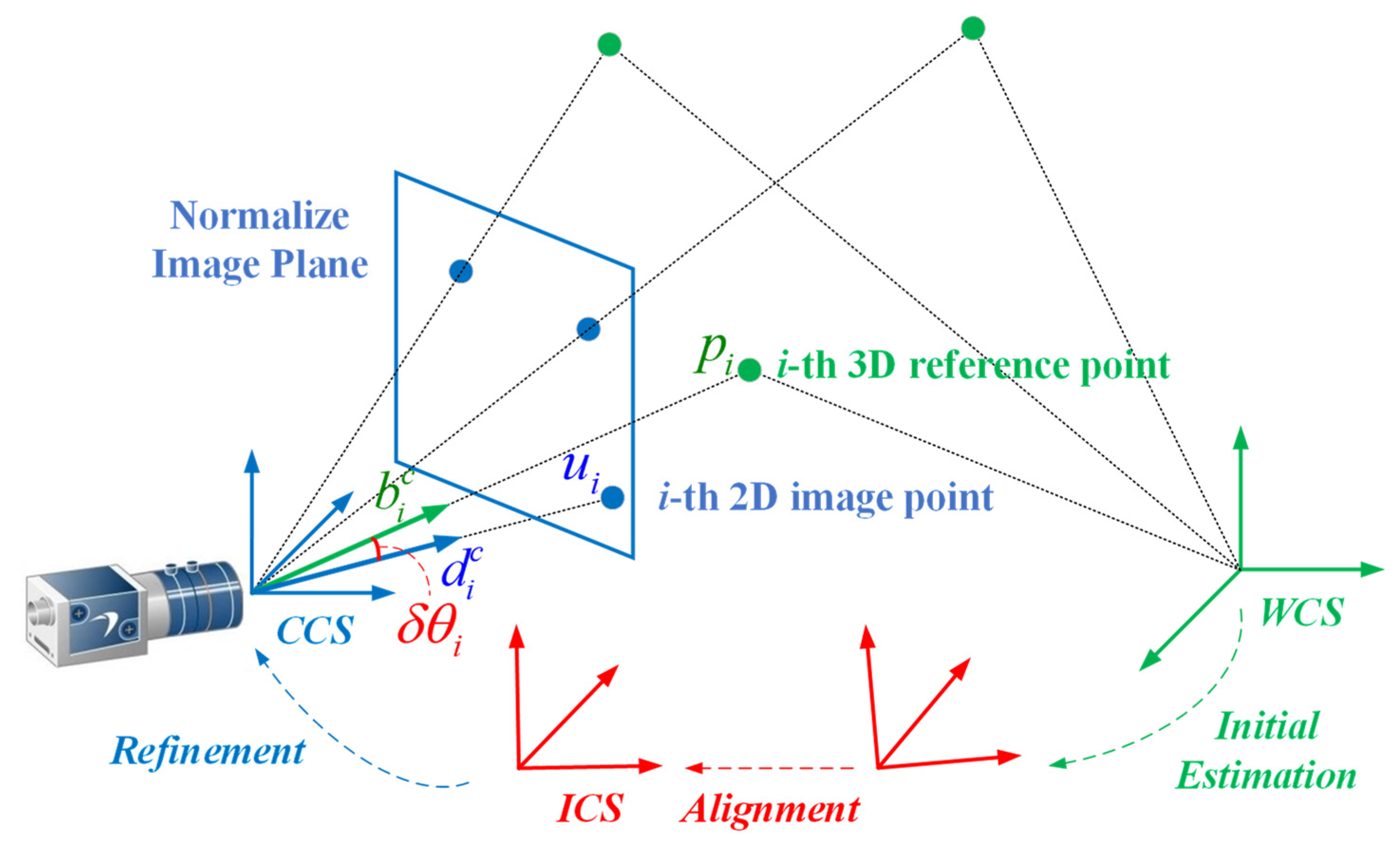
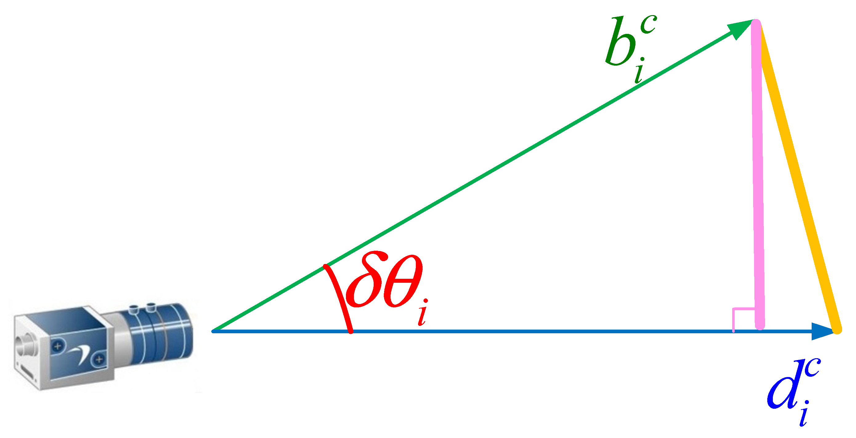
• Problem formulation—constructing the optimization with respect to δθ_i, enhanced by the Huber robust kernel;
• Initial estimation—roughly solving the PLD criterion by DLT to create a virtual ICS, which is close to the CCS;
• Alignment—aligning the ICS with the CCS under the small rotation assumption for the algorithm not to be trapped in periodic local minimums of δθ_i;
• Refinement—finally obtaining the rover pose with the global minimum of δθ_i.

2.1. Problem Formulation

First, the Huber kernel function is introduced to guarantee the convergence under gross measurements. Assuming $\delta {\theta }_i$ follows the Gaussian distribution [22], the Euclidean norm of $\delta {\theta }_i$ should be minimized. The overall algorithm is developed, as shown in Equation (1).

$$\left(R,t\right)=\mathrm{argmin}{\displaystyle \sum }_i\{\begin{array}{cc}2\epsilon \left|\delta {\theta }_i\right|-{\epsilon }^2& \left|\delta {\theta }_i\right|>\epsilon \\ \delta {\theta }_i^2& \left|\delta {\theta }_i\right|\le \epsilon \end{array}$$

(1)

where $\epsilon$ is the error threshold determined by measurement covariance. As shown in Figure 2, assuming $\delta {\theta }_i$ are small enough, they can be approximately expressed by the deviations between $b_i^c$ and $d_i^c$,

$$\delta {\theta }_i\approx \Vert b_i^c-d_i^c\Vert {}_2$$

(2)

Let $p_i^w$ and $p_i^c$ be the coordinates of $p_i$ in the WCS and CCS, which are indicated by superscribes w and c, respectively. The transformation from the WCS to the CCS can be defined as,

$$p_i^c=R{p}_i^w+t,$$

(3)

and $b_i^c$ can be normalized by

$$b_i^c=p_i^c/\Vert p_i^c\Vert {}_2,$$

(4)

where $\Vert ·\Vert {}_2$ denotes the Euclidean norm. Substituting Equations (2)–(4) into Equation (1), the optimization within the neighborhood of the angular minimum is obtained as

$$\left(R,t\right)=\mathrm{argmin}\left[-{\displaystyle \sum }_i\frac{1}{{\lambda }_i}{d}_i^c·\left(R{p}_i^w+t\right)\right]$$

(5)

where ${\lambda }_i=\Vert R{p}_i^w+t\Vert {}_2$ is the distance of the i-th point from the camera. The rover pose can be determined by $p_i^w$ and $d_i^c$, where $p_i^w$ are triangulated from previous views and $d_i^c$ are recovered from $u_i$ with calibrated intrinsics.

In the state-of-the-art literature [21], $\delta {\theta }_i$ is approximated by its sine value, while in our algorithm, Equation (2) is used. As illustrated in Figure 2, obviously, we adopt a closer approximation to calculate $\delta {\theta }_i$. As a result, our algorithm is more accurate. Moreover, our cost function is constructed with a lower order compared with the one in [21], which can be linearized more effectively in computations.

2.2. Initial Estimation

The PLD-based criterion is employed to obtain a linear estimation of rover pose. Without noise, all reference points should be located along their corresponding projection rays, which are originated from the optical center of the camera. The initial estimation of R and t can be derived using Equation (6).

$${\left[d_i^c\right]}_{\times }\left(R{p}_i^w+t\right)=0$$

(6)

where ${[·]}_{\times }$ is the corresponding skew-symmetric matrix of a vector.

The QR factorization of ${\left[d_i^c\right]}_{\times }$ is ${\left[d_i^c\right]}_{\times }=Q_{Di}{R}_{Di}$, where $Q_{Di}$ is orthogonal and $R_{Di}$ is upper triangular. The third element on the main diagonal of $R_{Di}$ is always zero. Therefore, the rank of ${\left[d_i^c\right]}_{\times }$ is 2 and the rows of ${\left[d_i^c\right]}_{\times }$ are linear dependent. ${\left[d_i^c\right]}_{\times }$ can be simplified as ${\left[d_i^c\right]}_{\times }^{-}$, which can be obtained in Equation (7).

$${\left[d_i^c\right]}_{\times }^{-}=\left[\begin{array}{ccc}1& 0& 0\\ 0& 1& 0\end{array}\right]·Q_{Di}$$

(7)

Although ${\left[d_i^c\right]}_{\times }^{-}$ has less dimensions than ${\left[d_i^c\right]}_{\times }$, it consists of the entire row basis of ${\left[d_i^c\right]}_{\times }$. Hence, ${\left[d_i^c\right]}_{\times }^{-}$ and ${\left[d_i^c\right]}_{\times }$ are equivalent in singular value decompositions (SVD), which lead to the same result in calculations. Because of the fewer dimensions used, the overall computing time is reduced, when using ${\left[d_i^c\right]}_{\times }^{-}$.

Base on Equation (6), t can be expressed by R as,

$$t=R_A^{-1}{Q}_A^{T}b$$

(8)

where $A=-{\left[\begin{array}{cc}\begin{array}{cc}{\left[d_1^c\right]}_{\times }^{-}& {\left[d_2^c\right]}_{\times }^{-}\end{array}& \begin{array}{cc}\cdots & {\left[d_n^c\right]}_{\times }^{-}\end{array}\end{array}\right]}^{\mathrm{T}}$, $b={\left[\begin{array}{cc}\begin{array}{cc}{\left[d_1^c\right]}_{\times }^{-}R{p}_1^w& {\left[d_2^c\right]}_{\times }^{-}R{p}_2^w\end{array}& \begin{array}{cc}\cdots & {\left[d_n^c\right]}_{\times }^{-}R{p}_n^w\end{array}\end{array}\right]}^{\mathrm{T}}$, and $Q_A$ and $R_A$ are the QR factorization of matrix A. The QR factorization introduced here is equivalent to the Moore–Penrose inverse when solving non-homogeneous linear equations. However, it is more robust for ill-conditioned equations and more efficient in calculations [23].

By substituting Equation (8) back into Equation (6), a homogeneous linear equation is obtained as,

$$Fx=0,$$

(9)

where $x={\left[\begin{array}{cc}\begin{array}{cc}{r}_{11}& r_{12}\end{array}& \begin{array}{cc}\cdots & r_{33}\end{array}\end{array}\right]}^{\mathrm{T}}$, which is composed of the nine elements in R, and F is the coefficient matrix computed from $p_i^w$ and $d_i^c$.

By relaxing the unit orthogonal constraints inherent in R and regarding x as independent variables, Equation (9) can be solved by SVD using at least 5 points,

$$F=US{V}^{\mathrm{T}}$$

(10)

and x is estimated to be $\widehat{x}$ as,

$$\widehat{x}=\left[\begin{array}{cc}{0}_{1\times 8}& 1\end{array}\right]V$$

(11)

The estimated rotation matrix $\widehat{R}$ can be recovered from $\widehat{x}$. The exploited constraints show that $\widehat{R}$ is not a correct rotation matrix. Therefore, $\widehat{R}$ should be projected to the SO(3) space. $\widehat{R}$ can be expressed by SVD as $\widehat{R}=U_1{S}_1{V}_1^{\mathrm{T}}$. The initial estimation of the rotation matrix, $R_{ini}$, can be found as,

$$R_{ini}=U_1{V}_1^{\mathrm{T}}$$

(12)

After obtaining the rotation matrix $R_{ini}$, the initial estimation of the translation vector, $t_{ini}$, can be computed by Equation (8).

Benefiting from the linear formulation, the reduced dimensions, and the QR factorization, the overall processing time is reduced. Unfortunately, because of the biased PLD criterion and the relaxation applied, the pose roughly estimated in this section cannot guarantee that the algorithm converges to the global angular minimum with the CCS directly, especially under large noise conditions. To solve this problem, the ICS is introduced and is further aligned with the CCS before the last step of iterative refinements.

2.3. Alignment

The ICS is then defined as the coordinate system generated by $R_{ini}$ and $t_{ini}$ and $p_i^m$ is denoted as the coordinate of the i-th reference point in the ICS. In this way, the ICS is only roughly initialized. Next, we further align the ICS with the CCS. The transformation in Equation (3) can be reorganized into homogeneous coordinates as,

$$\left[\begin{array}{c}{p}_i^c\\ 1\end{array}\right]=\left[\begin{array}{cc}{R}_{ali}& t_{ali}\\ 0& 1\end{array}\right]\left[\begin{array}{c}{p}_i^m\\ 1\end{array}\right]=\left[\begin{array}{cc}{R}_{ali}& t_{ali}\\ 0& 1\end{array}\right]\left[\begin{array}{cc}{R}_{ini}& t_{ini}\\ 0& 1\end{array}\right]\left[\begin{array}{c}{p}_i^w\\ 1\end{array}\right]$$

(13)

where $R_{ali}$ and $t_{ali}$ are the rotation matrix and the translation vector used for alignment, respectively.

Assuming that only a small transformation is required to align the ICS with the CCS, $R_{ali}$ can be approximately parameterized under small rotation conditions, i.e.,

$$R_{ali}=I+{\left[s_{ali}\right]}_{\times }$$

(14)

where $s_{ali}\in \mathfrak{s}\mathfrak{o}\left(3\right)$ is the Lie algebra. As you can see, there is no quadratic or trigonometric term in Equation (14), compared with the one using the Rodrigues formula in [21]. As a result, the algorithm used to calculate the pose can be converged quickly towards the global minimum, without being trapped in periodic local minimums. In addition, the linear expression here further reduces the computational time in this step.

Substituting Equation (14) into Equation (2), we have

$$\left[\frac{1}{\widehat{{\lambda }_i}}\begin{array}{cc}{\left[p_i^m\right]}_{\times }& -\frac{1}{\widehat{{\lambda }_i}}I\end{array}\right]\left[\begin{array}{c}{s}_{ali}\\ t_{ali}\end{array}\right]=\frac{1}{\widehat{{\lambda }_i}}{p}_i^m-d_i^c$$

(15)

where $\widehat{{\lambda }_i}=\Vert R_{ini}{p}_i^w+t_{ini}\Vert {}_2$ is the initial estimated distance of the i-th point from the camera. By utilizing the QR factorization, $s_{ali}$ can be easily solved. Subsequently, $R_{ali}$ can be calculated from the Rodrigues formula in Equation (16), and $t_{ali}$ can be retrieved from Equation (8).

$$R_{ali}=I+\sin \phi {\left[s_1\right]}_{\times }+\left(1-\cos \phi \right){\left[s_1\right]}_{\times }^2$$

(16)

where $\phi =\Vert s_{ali}\Vert {}_2$ and $s_1=s_{ali}/\Vert s_{ali}\Vert {}_2$.

2.4. Refinement

In this section, GN optimization is applied to refine the rover pose from the ICS to CCS, which is parameterized as the Lie algebra $l_k\in \mathfrak{s}\mathfrak{e}\left(3\right)$. The corresponding pose of $l_k$ can be calculated as,

$$\left[\begin{array}{cc}{R}_k& t_k\\ 0& 1\end{array}\right]=\exp \left({\left[l_k\right]}_{\times }\right)$$

(17)

where exp($·$) is the exponential function. The subscript k is introduced here to represent the k-th step during the refinements.

Next, the refinement $\Delta l_k$ is found to achieve the minimum $\delta {\theta }_i$ using the following normal equation,

$$H_k\Delta l_k=g_k,$$

(18)

where $H_k=\sum _i{J}_{i,k}^{\mathrm{T}}{J}_{i,k}$ is the Hessian matrix and $g_k=\sum _i{J}_{i,k}^{\mathrm{T}}{b}_{i,k}$. The Jacobian matrix $J_{i,k}$ is computed by

$$J_{i,k}=\frac{{\partial }_l\delta {\theta }_i}{{\partial }_l\mathsf{\Delta }{l}_k}=\left[\frac{1}{{\lambda }_{i,k}}{\left[p_{i,k}^m\right]}_{\times }\frac{1}{{\lambda }_{i,k}}(I-\frac{1}{{\lambda }_{i,k}^2}{p}_{i,k}^m{p}_{i,k}^{m\mathrm{T}})\right].$$

(19)

Compared with the Euler and CGR parameters, the Jacobian matrix given in Equation (19) is simpler in form [24]. The angular residual $b_{i,k}$ is calculated by

$$b_{i,k}=\frac{1}{{\lambda }_{i,k}}{p}_{i,k}^m-d_i^c.$$

(20)

With $\Delta l_k$ obtained, the pose can be updated by

$$\left[\begin{array}{cc}{R}_{k+1}& t_{k+1}\\ 0& 1\end{array}\right]=\exp \left({\left[\Delta l_k\right]}_{\times }\right)\left[\begin{array}{cc}{R}_k& t_k\\ 0& 1\end{array}\right].$$

(21)

It can be seen that Equation (19) has one more tensor term than Equation (15), $p_{i,k}^m{p}_{i,k}^{m\mathrm{T}}$, which is generated by the derivative of $1/{\lambda }_i$. Because of this additional term, the rover pose can be accurately refined to the angular minimum of $\delta {\theta }_i$. The pseudo-code of the proposed pose determination algorithm is summarized in Appendix A.

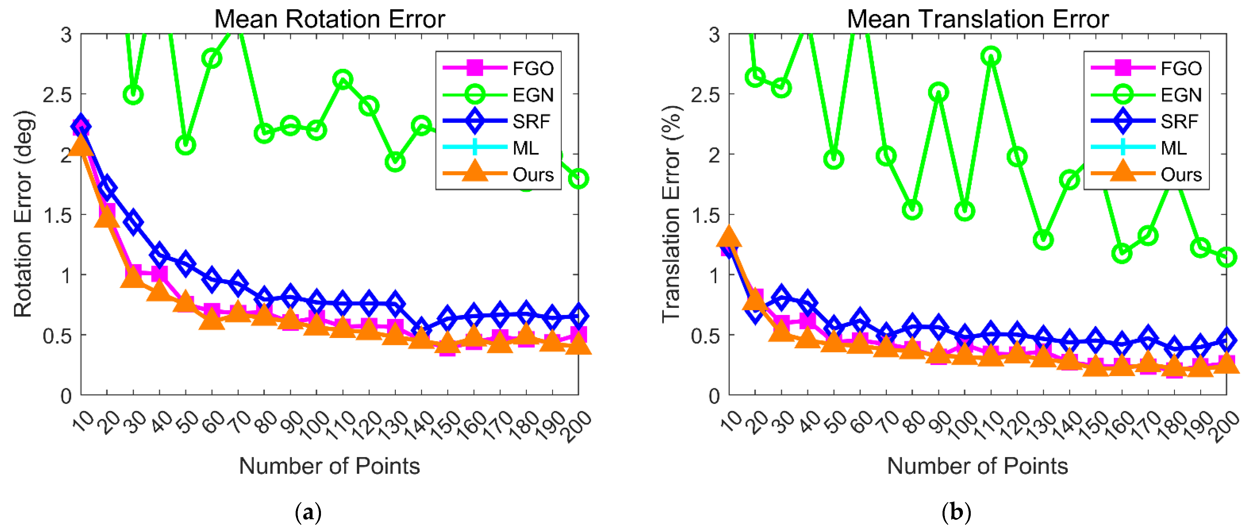
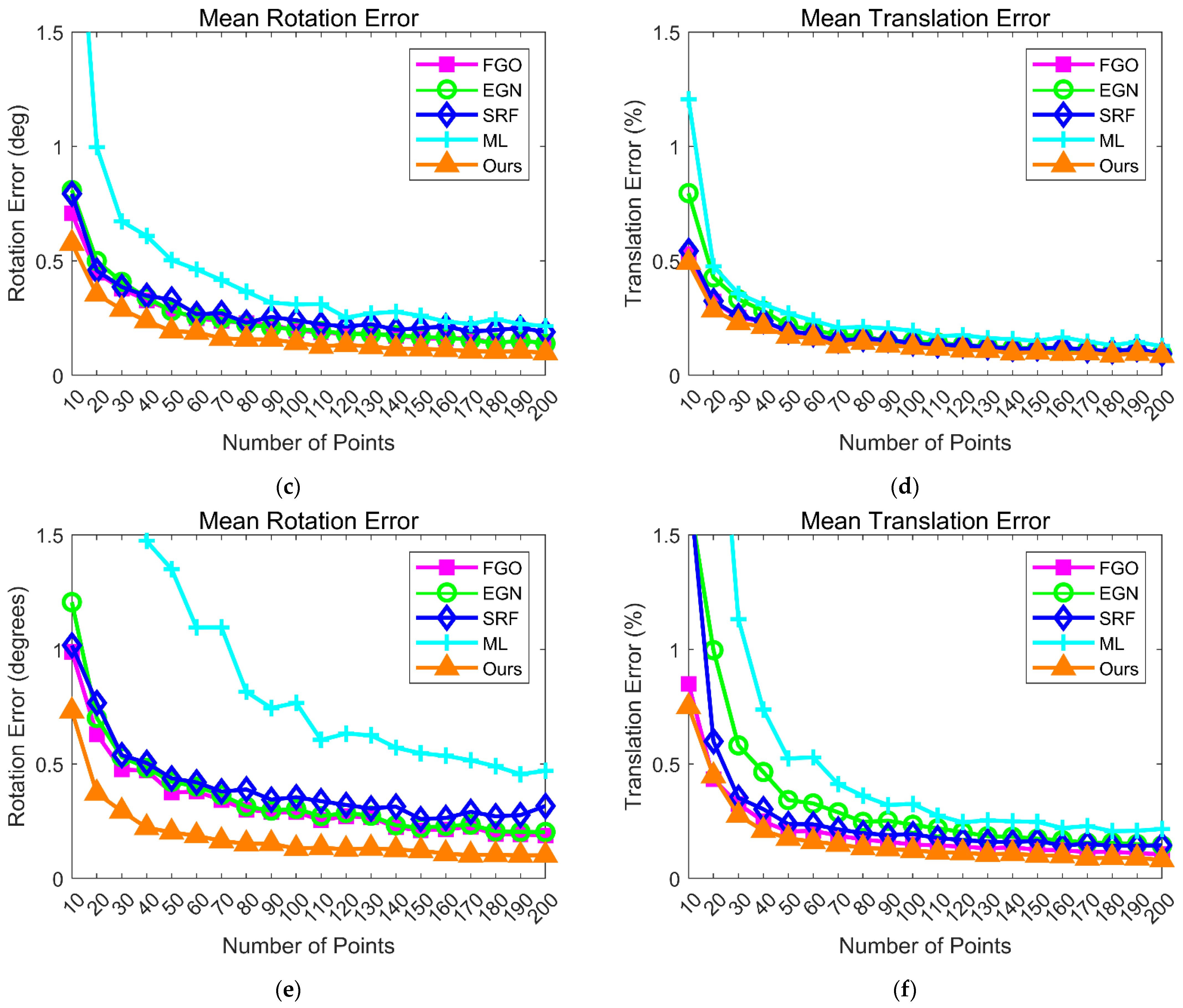
3. Implementations and Results

In this section, the proposed algorithm is implemented in synthetic and real environments. The rotation and translation errors are compared with those from the state-of-the-art pose estimators in each criterion [8,9,11,21], which are

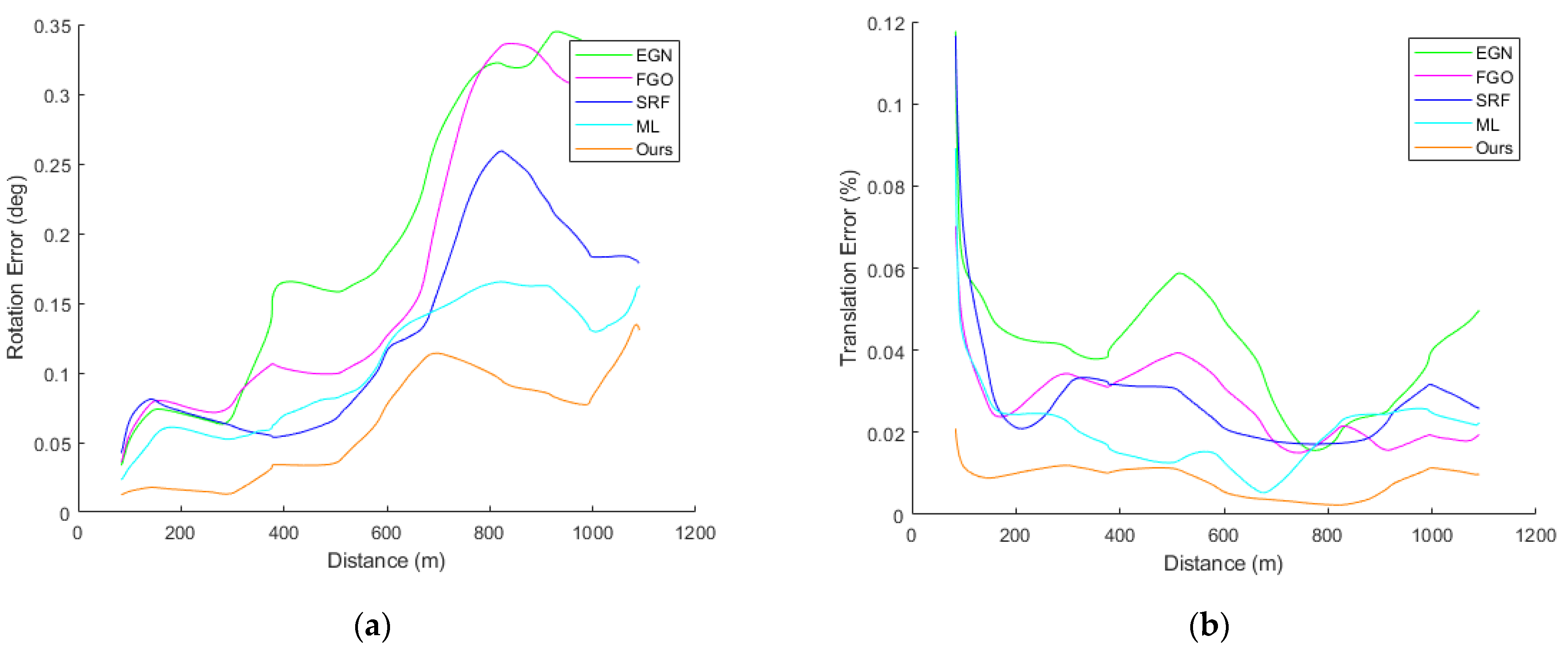
• The fast, general, and optimal algorithm (FGO) using the ATPC criterion [8];
• The efficient Gauss–Newton algorithm (EGN) using the PPD criterion [11];
• The simple, robust, and fast algorithm (SRF) using the PLD criterion [9];
• The maximum likelihood algorithm (ML) using the angle-based criterion [21].

The source codes of all the above four algorithms can be found from the references, respectively. All the simulations are done in MATLAB using a laptop with Intel(R) Core (TM) i5-3230M, 2.60 GHz CPU and 4.0 GB RAM.

Denote the ground-truth and the estimated pose as $\left(R_0,t_0\right)$ and $\left(R_e,t_e\right)$, respectively. The rotation error is defined as,

$$e_R=\arccos \left(\frac{\mathrm{tr}\left(R_e{R}_0^{\mathrm{T}}\right)-1}{2}\right)\times \frac{180}{\pi },$$

(22)

where tr($·$) is the trace of a matrix. The translation error is expressed as,

$$e_t=\frac{\Vert t_e-t_0\Vert {}_2}{\Vert t_0\Vert {}_2}\times 100\%.$$

(23)

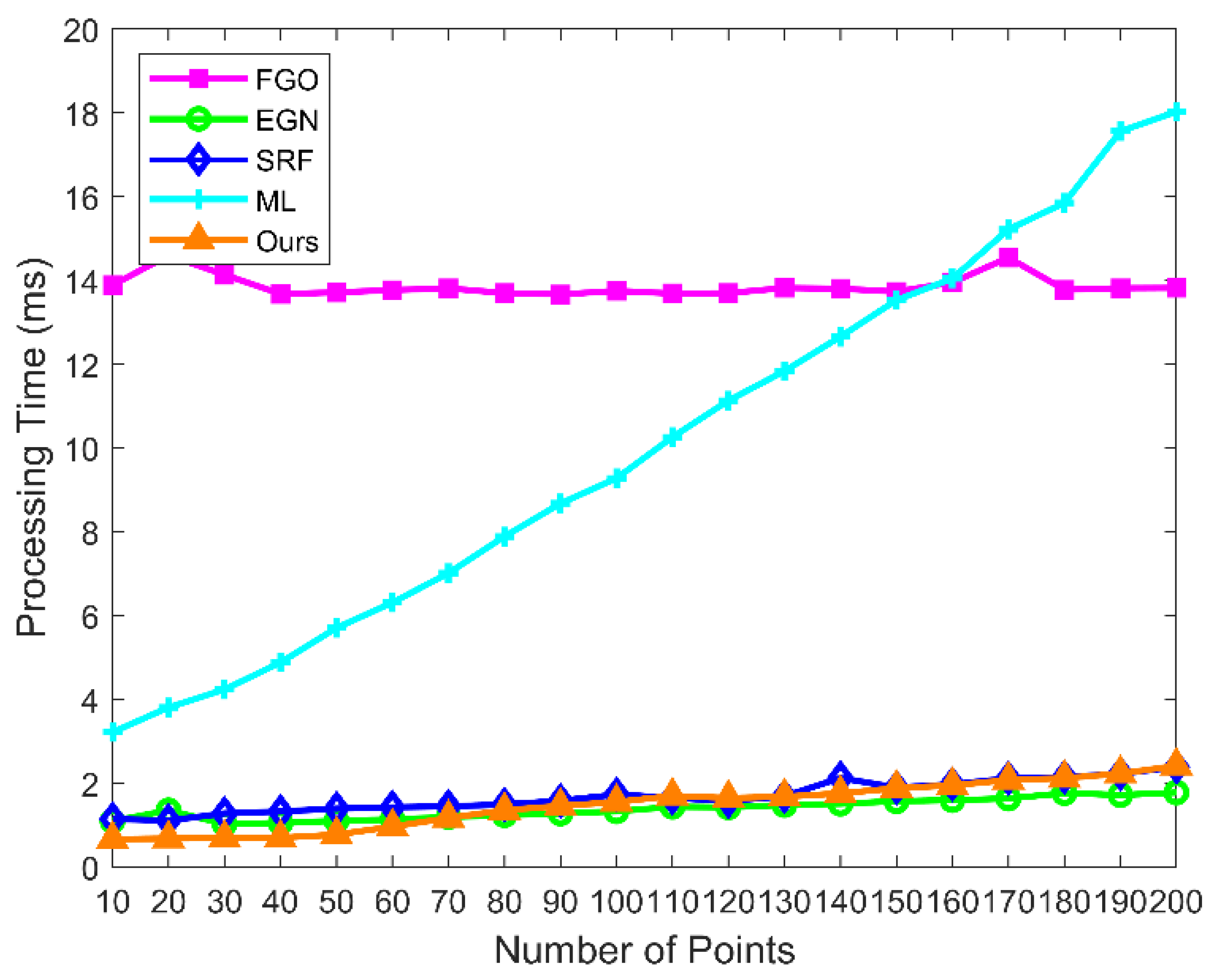
3.1. Synthetic Simulations

A virtual perspective camera is synthesized, whose focal length is set to be 500 pixels. N 3D reference points are generated in the CCS. These points are transformed into the WCS using the ground-truth poses, which are randomly sampled in the SE(3) space. Meanwhile, the 3D reference points are projected onto the image plane of the calibrated virtual camera and the Gaussian noises are added to these 2D image points.

3.1.1. Simulations in Known Environments

In this section, the planetary rover is set to move around the lander, which is considered as a known environment. In this situation, all the reference points have been well-calibrated without uncertainties. The measurement noises are the only source of noises.

Since the accuracy of the pose determination is closely related to the configuration of the reference points, different configurations should be synthesized to evaluate the performance of our proposed algorithm. Let $P={\left[\begin{array}{cc}\begin{array}{cc}{p}_1^w& p_2^w\end{array}& \begin{array}{cc}\cdots & p_N^w\end{array}\end{array}\right]}^{\mathrm{T}}$, then the distribution of the reference points can be described by the column rank $\gamma$ and the condition number $\kappa$ of $P$. Following the similar examples in [8,9,15,21], three configurations with different $\gamma$ and $\kappa$ values are used in the simulations:

• Planar configuration, with $\gamma =2$ and $\kappa \to \infty$. For example, the reference points are randomly distributed in the range of $\left[-2,2\right]\times \left[-2,2\right]\times \left[0,0\right]$;
• Ordinary configuration, with $\gamma =3$ and $\kappa \le 5$. For example, the reference points are randomly distributed in the range of $\left[-2,2\right]\times \left[-2,2\right]\times \left[2,6\right]$;
• Quasi-singular configuration, with $\gamma =3$ and $\kappa >5$. For example, the reference points are randomly distributed in the range of $\left[-2,2\right]\times \left[-2,2\right]\times \left[2,18\right]$.

First, the rotation and translation errors are investigated with respect to the number of reference points. N is varied from 10 to 200. The standard deviation of the Gaussian image noise is fixed at $\sigma =4$ pixels, in order to show the clear performance differences between our algorithm and the ones in the references. For each number of points, the simulation is repeated 500 times. The mean rotation and translation errors are reported in Figure 3.

It is well understood that the accuracy of pose determination increases with the number of points and decreases when the configuration of points becomes more singular, as illustrated in Figure 3. Our algorithm gives the best accuracies for all configurations. Especially, the greater advantages are shown from the planar to the ordinary and the quasi-singular configurations, where the distribution of the reference points becomes more discrete. In addition, as shown in Figure 4, the proposed algorithm is competitive in computational efficiency. Although an additional alignment step is added in our algorithm, we simplify the algorithm in each step. As a result, the overall processing time is not increased compared with the other algorithms. Moreover, from our simulations, it can be observed that the proposed algorithm uses the least time, when N < 80.

Second, the robustness is evaluated under different levels of noises. σ is varied from 0.5 to 5 pixels, while N is fixed at 50, which is the typical number in key-points selection [25]. For each level of noises, the simulation is repeated 500 times, and the mean rotation and translation errors are recorded in Figure 5.

As demonstrated in Figure 5, the accuracy of pose determination degrades with the increment of image noises. Among the evaluated algorithms, our algorithm is the least sensitive to Gaussian image noises, and it maintains the highest level of accuracies in all the synthesized configurations. Similarly, our algorithm shows the greatest improvements of accuracies in the quasi-singular case.

The above results confirm that our algorithm is the most accurate and robust for pose determinations, for all the configurations. The greatest improvements appear in the quasi-singular configuration, where the reference points are the most discrete. This is because, among all the algorithms, only the angle-based criterion considers measurement uncertainties related to the distances. Although ML also adopts the same angular criterion, it achieves less accurate pose determinations, compared with our algorithm. The reason is that ML is often trapped in local minimums because of its coarse initial pose estimation determined by the relaxed PLD criterion.

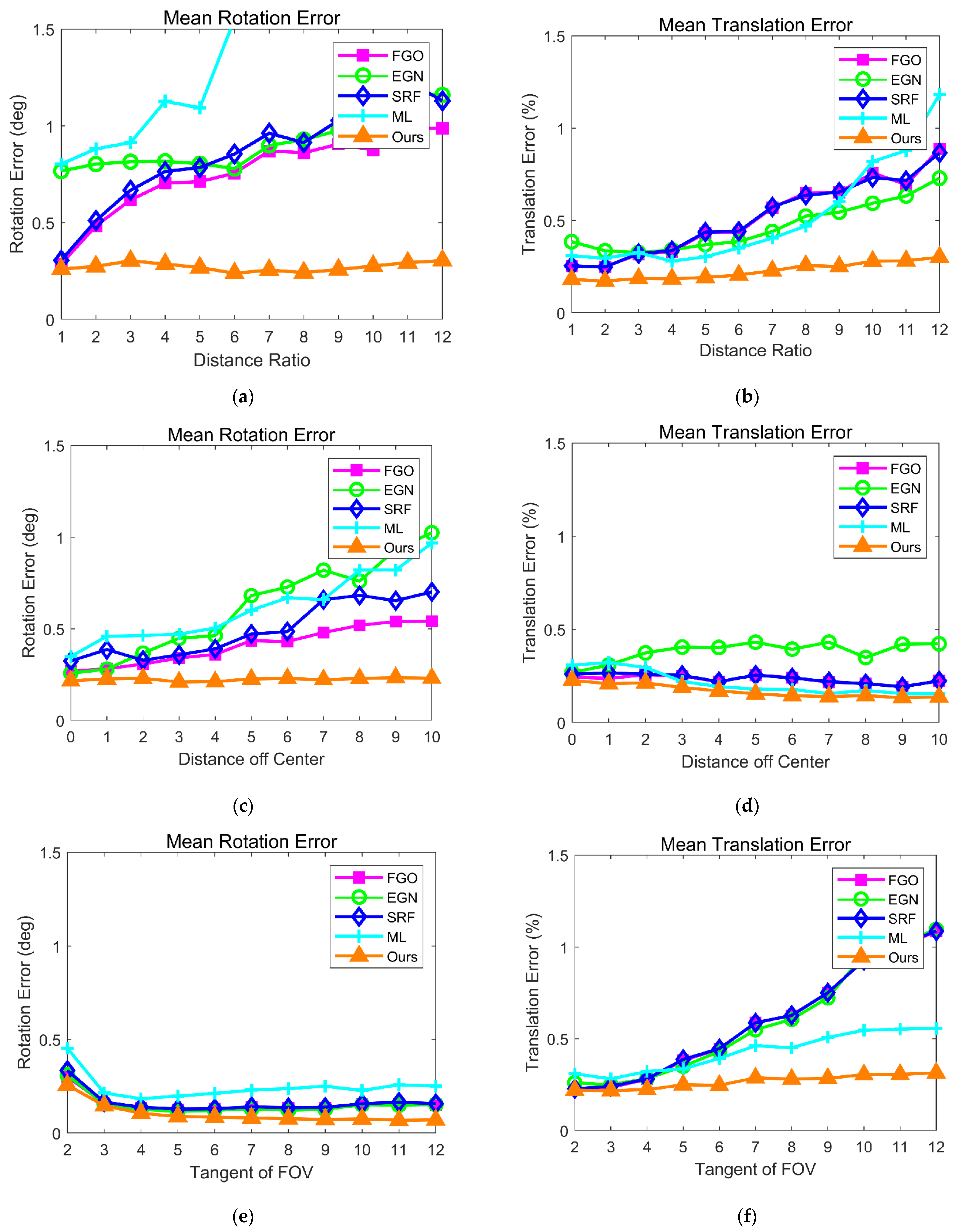
3.1.2. Simulations in Unknown Environments

In this section, the planetary rover is set to move in unknown environments, where the reference points are triangulated from previous views. This case represents the movement away from the lander. In this situation, both the uncertainties of the reference points and the measurement noises need to be considered.

Reconstructed by triangulations, the uncertainties of the 3D reference points increase with their squared distances from the camera but decrease with the number of the tracked views [26]. To show the effect of distances clearly, the reference points are triangulated by only two views around the current pose. The following scenarios are designed to validate the performance of our algorithm.

• The reference points are randomly distributed in the range of $\left[-2,2\right]\times \left[-2,2\right]\times \left[1,2r\right]$, where r is the distance ratio. r is varied from 1 to 12;
• The reference points are randomly distributed in the range of $\left[-2+o,2+o\right]\times \left[-2+o,2+o\right]\times \left[2,6\right]$, where o is the distance off center. o is varied from 0 to 10;
• The reference points are randomly distributed in the range of $\left[-q,q\right]\times \left[-q,q\right]\times \left[2,6\right]$, where q is the tangent of the field of view (FOV). q is varied from 2 to 12.

As can be seen here, the larger the value of r, o, and q, the more discrete the distribution of reference points.

During the simulations, N is fixed at 50, and σ is fixed at 2 pixels. All the simulations are repeated 500 times for each value of the parameters, and the mean rotation and translation errors are presented in Figure 6.

As illustrated in Figure 6, our algorithm shows the best accuracies in all the scenarios. Our accuracies remain almost unchanged, while the performances of FGO, EGN, SRF, and ML algorithms degrade, when the r, o, or q increases. It is observed in Figure 6a,b that, when r increases from 1 to 12, the rotation and translation errors using our algorithm are only changed from 0.26 to 0.29 degrees and from 0.18% to 0.29%, respectively. We can see the relatively rapid increments of the errors using the other algorithms. From Figure 6c,d it is found that the translation errors are less affected by the change of distance off center. When o increases from 0 to 10, the rotation error from our algorithm is kept around 0.22 degrees and this error grows greatly in the other algorithms. The rotation errors using the other algorithms are all above 0.54 degrees when o is 10. When the FOV increases, the rotation errors are likely not affected, as displayed in Figure 6e. Figure 6f shows that, the translation error from our algorithm remains below 0.31% while the errors are increased more than 0.55% using the other algorithms, when q reaches 12.

Overall, to our best knowledge, the proposed algorithm can achieve the most accurate pose determinations in all conditions of both known and unknown environments. Our algorithm is least influenced by the changes of distance ratio, distance off center, and FOV. The advantages of our algorithm are more obvious when used in an environment with larger distances and a wider FOV. Therefore, it suits the real implementation environments of planetary rovers the best.

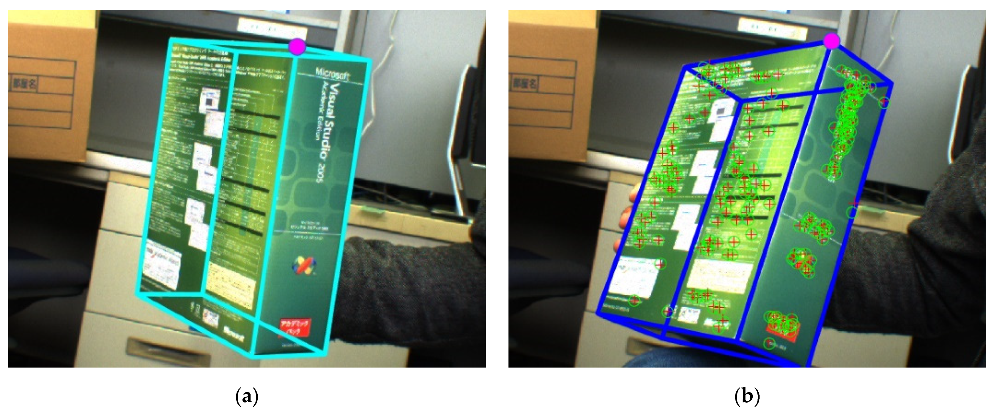
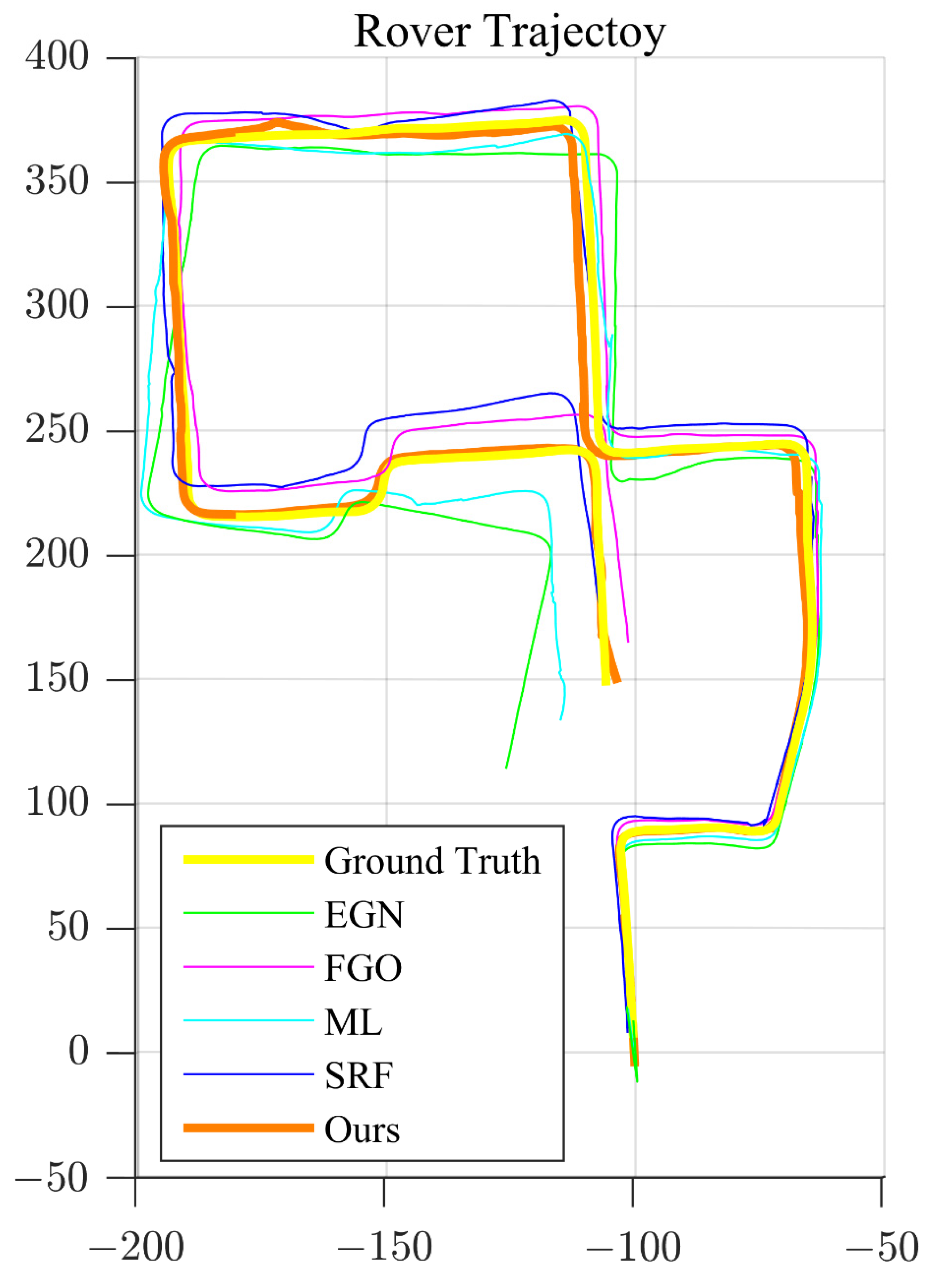
3.2. Real Experiments

3.2.1. Experiments in Known Environments

In this section, our algorithm is tested using the 3D box dataset [14]. First, the feature points in both the reference and current images are detected and extracted as scale-invariant feature transform (SIFT) points [27]. Then, these feature points are matched according to their Hamming distances, where the random sample consensus (RANSAC) method is employed for outlier removal [28]. The camera pose is calculated by these matched 3D-2D correspondences, using the above five algorithms, respectively. Finally, the 3D feature points are reprojected onto the 2D image plane using the determined poses and the average reprojection errors are calculated. The visual result using our algorithm is depicted in Figure 7, and the average reprojection errors are reported in

Table 1. The reprojection errors using the 3D box dataset.

Algorithm	FGO	EGN	SRF	ML	Ours
Reprojection Error (pixel)	1.634	5.420	1.642	3.476	1.604

.

As shown in Figure 7, since the reference points are in the ordinary configuration, the pose determined by our algorithm matches the reference image the best. However, compared with FGO and SRF, only small improvements are shown by our algorithm, due to the small distances and narrow FOV, as illustrated in Table 1.

3.2.2. Experiments in Unknown Environments

The KITTI dataset [29] is introduced to simulate the environment during the planetary exploration and the first 1500 frames of the left camera are used. Similarly, throughout the simulation, the feature points are extracted and matched as SIFT features, and the RANSAC method is employed for outlier elimination. The matched points are triangulated from previous views and tracked in the following frames. According to these 3D-2D correspondences, each pose estimator is used to determine the rover pose. Bundle adjustment is employed every 15 frames. The rover trajectories determined by each algorithm are presented in Figure 8 and the rotation and translation errors are shown in Figure 9.

As observed from Figure 8, due to the drift accumulated over time, the estimated trajectory gradually diverges from the ground truth for all compared algorithms. Our algorithm produces the smallest pose errors from the beginning to the end, as shown in Figure 9. These results are consistent with the above synthetic experiments. Because in real VO applications, taking the KITTI dataset as an example, the reference points are discretely distributed in the ordinary configuration, with large distances and wide FOV.

Besides, the average processing times of pose determinations per frame are 13.85 ms for FGO, 1.625 ms for EGN, 1.893 ms for SRF, 9.66 ms for ML, and 1.704 ms for our algorithm, respectively.

The above results verify that the proposed pose determination algorithm is the best for the planetary rover’s VO systems.

4. Conclusions

In this paper, an innovative pose determination algorithm based on the angular criterion was proposed for planetary rovers. The main novelty of this paper is to introduce the ICS, which greatly improves the alignment of the reference points from the WCS to the CCS. The algorithm was explained and verified in both synthetic and real environments. The simulation results confirmed that the proposed algorithm provides the most accurate pose determinations compared with the other state-of-the-art algorithms, especially in an environment with large distance and wide FOV.

Limitations and future improvements. As discussed in Section 3, there are two major limitations of our algorithm. The first one is that our algorithm only shows great advantages in a configuration with large distances and a wide FOV. The second one is that the time consumption for the additional alignment step becomes obvious when the number of points is more than 80. Therefore, the future improvements will mainly focus on a more efficient implementation of the angle-based criterion in dense feature scenarios.

References

1. Andolfo, S.; Petricca, F.; Genova, A. Rovers Localization by using 3D-to-3D and 3D-to-2D Visual Odometry. In Proceedings of the IEEE 8th International Workshop on Metrology for AeroSpace, Naples, Italy, 23–25 June 2021. [Google Scholar]
2. Chiodini, S.; Giubilato, R.; Pertile, M.; Salvioli, F.; Bussi, D.; Barrera, M.; Franceschetti, P.; Debei, S. Viewpoint Selection for Rover Relative Pose Estimation Driven by Minimal Uncertainty Criteria. IEEE Trans. Instrum. Meas. 2021, 70, 1–12. [Google Scholar] [CrossRef]
3. Ma, Y.; Liu, S.; Sima, B.; Wen, B.; Peng, S.; Jia, Y. A precise visual localisation method for the Chinese Chang’e-4 Yutu-2 rover. Photogramm. Rec. 2020, 35, 10–39. [Google Scholar] [CrossRef]
4. Maki, J.N.; Gruel, D.; McKinney, C.; Ravine, M.A.; Morales, M.; Lee, D.; Willson, R.; Copley-Woods, D.; Valvo, M.; Goodsall, T.; et al. The Mars 2020 Engineering Cameras and Microphone on the Perseverance Rover: A Next-Generation Imaging System for Mars Exploration. Space Sci. Rev. 2020, 216, 1–48. [Google Scholar] [CrossRef] [PubMed]
5. Winter, M.; Barcaly, C.; Pereira, V.; Lancaster, R.; Caceres, M.; Mcmanamon, K.; Nye, B.; Silva, N.; Lachat, D.; Campana, M. ExoMars Rover Vehicle: Detailed Description of the GNC System. In Proceedings of the 13th Symposium on Advanced Space Technologies in Robotics and Automation, Noordwijk, The Netherlands, 11–13 May 2015. [Google Scholar]
6. Shao, W.; Cao, L.; Guo, W.; Xie, J.; Gu, T. Visual navigation algorithm based on line geomorphic feature matching for Mars landing. Acta Astronaut. 2020, 173, 383–391. [Google Scholar] [CrossRef]
7. Haralick, R.M.; Lee, C.N.; Ottenburg, K.; Nölle, M. Analysis and Solutions of The Three Point Perspective Pose Estimation Problem. In Proceedings of the IEEE Computer Society Conference on Computer Vision and Pattern Recognition, Maui, HI, USA, 3–6 June 1991. [Google Scholar]
8. Li, S.; Xu, C.; Xie, M. A Robust O(n) Solution to the Perspective-n-Point Problem. IEEE Trans. Pattern Anal. Mach. Intell. 2012, 34, 1444–1450. [Google Scholar] [CrossRef] [PubMed]
9. Wang, P.; Xu, G.; Cheng, Y.; Yu, Q. A simple, robust and fast method for the perspective-n-point Problem. Pattern Recognit. Lett. 2018, 108, 31–37. [Google Scholar] [CrossRef]
10. Garro, V.; Crosilla, F.; Fusiello, A. Solving the PnP Problem with Anisotropic Orthogonal Procrustes Analysis. In Proceedings of the 2nd International Conference on 3D Imaging, Modeling, Processing, Visualization & Transmission, Zurich, Switzerland, 13–15 October 2012. [Google Scholar]
11. Moreno-Noguer, F.; Lepetit, V.; Fua, P. Accurate Non-Iterative O(n) Solution to PnP Problem. In Proceedings of the IEEE 11th International Conference on Computer Vision, Rio de Janeiro, Brazil, 14–21 October 2007. [Google Scholar]
12. Ferraz, L.; Binefa, X.; Moreno-Noguer, F. Very Fast Solution to the PnP Problem with Algebraic Outlier Rejection. In Proceedings of the IEEE Conference on Computer Vision and Pattern Recognition, Columbus, IN, USA, 23–28 June 2014. [Google Scholar]
13. Ferraz, L.; Binefa, X.; Moreno-Noguer, F. Leveraging Feature Uncertainty in the PnP Problem. In Proceedings of the British Machine Vision Conference, Nottingham, UK, 1–5 September 2014. [Google Scholar]
14. Zheng, Y.; Kuang, Y.; Sugimoto, S.; Astrom, K.; Okutomi, M. Revisiting the PnP Problem: A Fast, General and Optimal Solution. In Proceedings of the IEEE International Conference on Computer Vision, Sydney, Australia, 1–8 December 2013. [Google Scholar]
15. Yu, Q.; Xu, G.; Zhang, L.; Shi, J. A consistently fast and accurate algorithm for estimating camera pose from point correspondences. Measurement 2021, 172, 108914. [Google Scholar] [CrossRef]
16. Hartley, R.; Zisserman, A. Multiple View Geometry in Computer Vision, 2nd ed.; Cambridge University Press: Cambridge, UK, 2003; pp. 146–157. [Google Scholar]
17. Martinez, G. Field tests on flat ground of an intensity-difference based monocular visual odometry algorithm for planetary rovers. In Proceedings of the 15th IAPR International Conference on Machine Vision Applications, Nagoya, Japan, 8–12 May 2017. [Google Scholar]
18. Li, H.; Chen, L.; Li, F. An Efficient Dense Stereo Matching Method for Planetary Rover. IEEE Access 2019, 7, 48551–48564. [Google Scholar] [CrossRef]
19. Corke, P.; Strelow, D.; Singh, S. Omnidirectional visual odometry for a planetary rover. In Proceedings of the IEEE/RSJ International Conference on Intelligent Robots and Systems, Sendai, Japan, 28 September–2 October 2004. [Google Scholar]
20. Hesch, J.A.; Roumeliotis, S.I. A Direct Least-Squares (DLS) method for PnP. In Proceedings of the IEEE International Conference on Computer Vision, Barcelona, Spain, 6–13 November 2011. [Google Scholar]
21. Urban, S.; Leitloff, J.; Hinz, S. MLPnP-a real-time maximum likelihood solution to the perspective-n-point problem. In Proceedings of the ISPRS Annals of the Photogrammetry, Remote Sensing and Spatial Information Sciences, Prague, Czech, 12–19 July 2016. [Google Scholar]
22. Yang, K.; Fang, W.; Zhao, Y.; Deng, N. Iteratively Reweighted Midpoint Method for Fast Multiple View Triangulation. IEEE Robot. Autom. Lett. 2019, 4, 708–715. [Google Scholar] [CrossRef]
23. Takeshi, F.; Ramaseshan, K.; Yuji, N.; Yusaku, Y.; Yuka, Y. Shifted Cholesky QR for Computing the QR Factorization of Ill-Conditioned Matrices. SIAM J. Sci. Comput. 2020, 42, 477–503. [Google Scholar]
24. Mangelson, J.G.; Ghaffari, M.; Vasudevan, R.; Eustice, R.M. Characterizing the Uncertainty of Jointly Distributed Poses in the Lie Algebra. IEEE Trans. Robot. 2020, 36, 1371–1388. [Google Scholar] [CrossRef]
25. Zhao, Y.; Vela, P.A. Good Feature Matching: Toward Accurate, Robust VO/VSLAM with Low Latency. IEEE Trans. Robot. 2020, 36, 657–675. [Google Scholar] [CrossRef] [Green Version]
26. Zhou, B.; Luo, S.; Zhang, S. Pre-Weighted Midpoint Algorithm for Efficient Multiple-View Triangulation. IEEE Robot. Autom. Lett. 2021, 6, 7839–7845. [Google Scholar]
27. Lowe, D.G. Distinctive Image Features from Scale-Invariant Keypoints. Int. J. Comput. Vis. 2004, 60, 91–110. [Google Scholar] [CrossRef]
28. Fischler, M.A.; Bolles, R.C. Random sample consensus: A paradigm for model fitting with applications to image analysis and automated cartography. Commun. ACM 1981, 24, 381–395. [Google Scholar] [CrossRef]
29. Geiger, A.; Lenz, P.; Urtasun, R. Are We Ready for Autonomous Driving? The KITTI Vision Benchmark Suite. In Proceedings of the IEEE Conference on Computer Vision and Pattern Recognition, Providence, RI, USA, 16–21 June 2012. [Google Scholar]
Figure 1. Formulation of pose determination. Note that, although a perspective camera is used here, the proposed algorithm can be used for any type of central cameras.
Aerospace 09 00391 g001
Figure 2. Approximation of δθi. δθi is enlarged to show the difference clearly. The approximation in our algorithm is colored in orange while the one in [21] is colored in pink.
Aerospace 09 00391 g002
Figure 3. The accuracies of pose determinations with respect to the number of reference points. (a,b) are in the planar configuration; (c,d) are in the ordinary configuration; and (e,f) are in the quasi-singular configuration, respectively.
Aerospace 09 00391 g003aAerospace 09 00391 g003b
Figure 4. The processing times in the ordinary configuration, corresponding to Figure 3c,d.
Aerospace 09 00391 g004
Figure 5. The accuracies of pose determinations with respect to the Gaussian image noise. (a,b) are in the planar configuration; (c,d) are in the ordinary configuration; and (e,f) are in the quasi-singular configuration, respectively.
Aerospace 09 00391 g005
Figure 6. The accuracies of pose determinations with respect to (a,b) the distance ratio, (c,d) the distance off center, and (e,f) the tangent of FOV, respectively.
Aerospace 09 00391 g006
Figure 7. The visual result of our proposed algorithm on the 3D box dataset. (a) is the reference image, and (b) is the current image augmented by the reprojected contour. The red cross marks are the feature points matched with the reference image, and the green circle marks are the reprojected features points using the determined camera pose.
Aerospace 09 00391 g007
Figure 8. The determined trajectories of the planetary rover. The ground truth and our determined trajectories are bolded.
Aerospace 09 00391 g008
Figure 9. The pose determination errors of the planetary rover with respect to the travel distances, where (a) is rotation errors and (b) is translation errors.
Aerospace 09 00391 g009