High-Order CFD Solvers on Three-Dimensional Unstructured Meshes: Parallel Implementation of RKDG Method with WENO Limiter and Momentum Sources

Abstract

In aerospace engineering, high-order computational fluid dynamics (CFD) solvers suitable for three-dimensional unstructured meshes are less developed than expected. The Runge–Kutta discontinuous Galerkin (RKDG) finite element method with compact weighted essentially non-oscillatory (WENO) limiters is one of the candidates, which might give high-order solutions on unstructured meshes. In this article, we provide an efficient parallel implementation of this method for simulating inviscid compressible flows. The implemented solvers are tested on lower-dimensional model problems and real three-dimensional engineering problems. Results of lower-dimensional problems validate the correctness and accuracy of these solvers. The capability of capturing complex flow structures even on coarse meshes is shown in the results of three-dimensional applications. For solving problems containing rotary wings, an unsteady momentum source model is incorporated into the solvers. Such a finite element/momentum source hybrid method eliminates the reliance on advanced mesh techniques, which might provide an efficient tool for studying rotorcraft aerodynamics.

1. Introduction

Computational fluid dynamics (CFD) solvers, widely used in aerospace engineering, are based either on finite difference (FD) schemes or on finite volume (FV) schemes. However, FD schemes are restricted on structured meshes, while most FV schemes have only first- or second-order accuracy. One way to develop higher-order schemes suitable for unstructured meshes is to use the discontinuous Galerkin (DG) finite element (FE) methods. As with other FE methods, DG methods assume continuous approximation in each element (i.e., cell). However, they allow discontinuities to exist on intercell boundaries. Such discontinuities are then resolved by numerical fluxes, e.g., exact or approximate Riemann solvers, as with Godunov-type schemes [1]. The original DG scheme was not proposed for CFD but for solving the linear neutron transport equation [2]. For nonlinear conservation laws, Chavent and Salzano [3] designed an explicit Euler DG cheme, which is second-order accurate in space but only first-order accurate in time. To improve the accuracy of time discretization, Cockburn and Shu [4] replaced the first-order forward Euler method with high-order Runge–Kutta (RK) methods, which led to the family of Runge–Kutta discontinuous Galerkin (RKDG) schemes for scalar conservation laws [5,6], for one-dimensional conservation law systems [7], for multi-dimensional scalar conservation laws [8] and for multi-dimensional conservation law systems [9]. The last case includes the Euler system that depicts inviscid compressible flows, which is the first application of RKDG in CFD. We will give a concise derivation of this scheme in Section 2.1 and Section 2.2.

The Euler system is hyperbolic, and might have discontinuities in its solutions. Approximating such solutions with finite terms of continuous functions would generate numerical oscillations near discontinuities (known as the Gibbs phenomenon [10]). Therefore, any useful high-order scheme must incorporate some mechanism for suppressing such spurious oscillations. For second-order FD and FV schemes, there are slope and flux limiters [11]. These limiters work well on shock capturing but might reduce the order of accuracy when used in smooth regions. Furthermore, they are not applicable to higher-order schemes. To overcome these drawbacks, the essentially non-oscillatory (ENO) [12] and weighted ENO (WENO) [13] limiters for high-order FD schemes, which can essentially suppress spurious oscillations and maintain high-order accuracy in smooth regions, were developed. Similar ideas were later incorporated into FV [14] and DG [15,16] schemes, which are suitable for unstructured meshes. However, such early versions of unstructured WENO limiters have to query not only a cell’s immediate neighbors, but also the neighbors’ neighbors, and so on. To preserve the compactness of RKDG schemes, Zhong [17] and Zhu [18] proposed a compact WENO limter for two-dimensional structured and unstructrued meshes. In our early work [19], we extended it to three-dimensional and presented an efficient parallel implementation. We will summarize the key steps of this compact WENO limiter in Section 2.3.

The parallel implementation of the RKDG scheme with a compact WENO limiter can be used for solving many practical problems in aerospace engineering. However, for problems with moving boundaries (such as rotary wings on a helicopter or blades on a wind turbine), advanced meshing techniques (such as dynamic meshing, overset meshes or adaptive mesh refinement) have to be applied. On the other hand, typical lifting bodies (such as rotary wings) have been successfully modeled as various momentum sources in FD/FV schemes. Rajagopalan and Mathur [20,21] proposed the first FD/FV-based momentum source model, which models the time-averaged effect of a rotor as an actuator disk. Such a steady model was used by Kang and Sun [22,23] for solving the flow fields of rotors in ground effect. Shi [24] compared this model with an unsteady overset mesh method, and found that the steady momentum source model can predict complex aerodynamic interactions between a rotor and a flight deck at a much cheaper cost. Shen [25] and Kim [26] refined the model by replacing the actuator disk for the entire rotor with an actuator surface for each blade of the rotor, so that unsteady effects of rotary wings can be captured. Such early works are either oversimplified by ignoring unsteady effects (such as [20,21,22,23]), or restricted to structured meshes (such as [24,25]). To overcome these drawbacks, our parallel RKDG solvers are augmented with an unsteady actuator line model, which successfully captures unsteady effects of a rotor on unstructured meshes. The formulation of this finite element/momentum source hybrid method will be given in Section 2.4. Some demonstrative results are presented in Section 3.3.

2. The RKDG Method with WENO Limiters and Momentum Sources

Mathematically, the problems that we are going to solve in Section 3 are defined by the three-dimensional Euler system

$${\partial }_t\left[\begin{array}{c}\rho \\ \rho u_x\\ \rho u_y\\ \rho u_z\\ \rho e_0\end{array}\right]+{\partial }_x\left[\begin{array}{c}\rho u_x\\ \rho u_x{u}_x+p\\ \rho u_y{u}_x\\ \rho u_z{u}_x\\ \rho h_0{u}_x\end{array}\right]+{\partial }_y\left[\begin{array}{c}\rho u_y\\ \rho u_x{u}_y\\ \rho u_y{u}_y+p\\ \rho u_z{u}_y\\ \rho h_0{u}_y\end{array}\right]+{\partial }_z\left[\begin{array}{c}\rho u_z\\ \rho u_x{u}_z\\ \rho u_y{u}_z\\ \rho u_z{u}_z+p\\ \rho h_0{u}_z\end{array}\right]=\left[\begin{array}{c}0\\ b_x\\ b_y\\ b_z\\ 0\end{array}\right]$$

(1)

with certain boundary and initial conditions, which describes inviscid compressible flows. In Equation (1),

• Variables in the first column are called conservative variables;
• The density $\rho$, the velocity components $u_x,u_y,u_z$ and the pressure p are called primitive variables;
• The thermodynamic quantities $e_0$ and $h_0$ are the specific total energy and the specific total enthalpy, respectively; for ideal gases, they can be written as functions of the five primitive variables:

  $$e_0=\frac{p/\rho }{\gamma -1}+\frac{u_x^2+u_y^2+u_z^2}{2},h_0=e_0+\frac{p}{\rho },$$

  in which $\gamma$ is the heat capacity ratio of the gas, and we use $\gamma =1.4$ in this article;
• The body force components $b_x,b_y,b_z$ are assumed to be 0s, except in Section 3.3.

The method that we use for solving the Euler system (1) is the RKDG method with a WENO limiter. A detailed formulation of this method for sourceless problems has been given in our previous work [19]. In this section, we give a more complete formulation, which takes source terms into consideration. If all source terms were canceled, it would reduce to the form in [19].

2.1. The DG Space Discretization

Equation (1) can be written as

$${\partial }_t\underline{U}+\nabla ·\underline{\overrightarrow{F}}=\underline{Q},$$

(2)

in which $\underline{\overrightarrow{F}}=\underline{F^x}{\overrightarrow{e}}_x+\underline{F^y}{\overrightarrow{e}}_y+\underline{F^z}{\overrightarrow{e}}_z$ is the flux vector whose components $\underline{F^x}$, $\underline{F^y}$, $\underline{F^z}$, and $\underline{U}$, $\underline{Q}$ are all $5\times 1$ matrices, each row of which is a scalar function depending on position $\overrightarrow{x}$ and time t. By multiplying both sides with an arbitrary test function $\psi (\overrightarrow{x})$ and integrating the products on the i-th element (i.e., cell) $E_i$, and applying integral by parts and Gauss’s divergence theorem, Equation (2) can be turned into a weak form:

$${\int }_{E_i}\left(\psi {\partial }_t\underline{U}-\underline{\overrightarrow{F}}·\nabla \psi \right)+{\int }_{\partial E_i}\left(\overrightarrow{\nu }·\underline{\overrightarrow{F}}\right)\psi ={\int }_{E_i}\underline{Q}\psi ,$$

(3)

where $\overrightarrow{\nu }$ is the outer normal unit vector of $\partial E_i$ (which is the boundary of E).

By choosing an orthonormal basis of the linear space spanned by polynomials less than the p-th degree over E, denoted as $\underline{\varphi }(\overrightarrow{x}):=\left[\begin{array}{ccc}{\varphi }_1(\overrightarrow{x})& \dots & {\varphi }_L(\overrightarrow{x})\end{array}\right]$, the unknowns $\underline{U}$ and the arbitrary test function $\psi$ can be approximated as

$$\underline{U}(\overrightarrow{x},t)\approx {\underline{U}}^h(\overrightarrow{x},t)=\sum _{l=1}^L{\widehat{\underline{U}}}_l\left(t\right){\varphi }_l\left(\overrightarrow{x}\right),\psi \left(\overrightarrow{x}\right)\approx {\psi }^h\left(\overrightarrow{x}\right)=\sum _{l=1}^L{\widehat{\psi }}_l{\varphi }_l\left(\overrightarrow{x}\right),$$

in which each ${\widehat{\underline{U}}}_l\left(t\right)$ is a $5\times 1$ matrix of temporal functions, and each ${\widehat{\psi }}_l$ is an arbitrary constant number. Substituting them into the weak form (Equation 2) gives

$$\sum _l{\widehat{\psi }}_l\left[\sum _k\left({\int }_{E_i}{\varphi }_l{\varphi }_k\right)\frac{\mathrm{d}{\underline{\widehat{U}}}_k}{\mathrm{d}t}+{\int }_{E_i}\left(\underline{\overrightarrow{F}}·\nabla {\varphi }_l-\underline{Q}{\varphi }_l\right)+{\oint }_{\partial E_i}{\varphi }_l\underline{F^{\nu }}\right]=\underline{O},$$

(4)

where $\overrightarrow{\nu }·\underline{\overrightarrow{F}}=:\underline{F^{\nu }}$ is the normal flux at some point on $\partial E_i$, whose value could be given by an exact or approximate Riemann solver of Equation (2); see [27] for details.

Recall the arbitrariness of ${\left\{{\widehat{\psi }}_l\right\}}_{l=1}^L$ and adopt the inner product notation

$$\langle f|g\rangle :={\int }_{E_i}f\left(\overrightarrow{x}\right)g\left(\overrightarrow{x}\right),$$

and we could turn Equation (4) into a system of ordinary differential equations:

$$\frac{\mathrm{d}\underline{\widehat{U}}}{\mathrm{d}t}=\underline{R}\left(\underline{\widehat{U}}\right),$$

(5)

in which

$$\underline{\widehat{U}}\left(t\right)=\left[\begin{array}{ccc}\langle U_1|{\varphi }_1\rangle & \dots & \langle U_1|{\varphi }_L\rangle \\ ⋮& \ddots & ⋮\\ \langle U_5|{\varphi }_1\rangle & \dots & \langle U_5|{\varphi }_L\rangle \end{array}\right]$$

is a $5\times L$ matrix of temporal functions (which will be solved in Section 2.2), and 

$$\underline{R}={\int }_{E_i}\left(\left[\begin{array}{ccc}\underline{F^x}& \underline{F^y}& \underline{F^z}\end{array}\right]\left[\begin{array}{c}{\partial }_x\underline{\varphi }\\ {\partial }_y\underline{\varphi }\\ {\partial }_z\underline{\varphi }\end{array}\right]-\underline{Q}\underline{\varphi }\right)-{\oint }_{\partial E_i}\underline{F^{\nu }}\underline{\varphi }$$

(6)

is a variable matrix depending on $\underline{\widehat{U}}$. The integrals in Equation (6) are evaluated by Gaussian quadrature rules, such as those given by [28].

2.2. The RK Time Discretization

Equation (5) is a typical system of nonlinear ordinary differential equations. In this article, we use the following explicit Runge–Kutta methods:

first-order: 

$$\begin{array}{cc}\hfill {\underline{\widehat{U}}}^{n+1}& ={\underline{\widehat{U}}}^n+{\underline{R}}^n\Delta t;\hfill \end{array}$$

second-order: 

$$\begin{array}{cc}\hfill {\underline{\widehat{U}}}^{n+1/2}& ={\underline{\widehat{U}}}^n+{\underline{R}}^n\Delta t,\hfill \\ \hfill {\underline{\widehat{U}}}^{n+1}\equiv {\underline{\widehat{U}}}^{n+2/2}& =\frac{1}{2}{\underline{\widehat{U}}}^n+\frac{1}{2}\left({\underline{\widehat{U}}}^{n+1/2}+{\underline{R}}^{n+1/2}\Delta t\right);\hfill \end{array}$$

third-order: 

$$\begin{array}{cc}\hfill {\underline{\widehat{U}}}^{n+1/3}& ={\underline{\widehat{U}}}^n+{\underline{R}}^n\Delta t,\hfill \\ \hfill {\underline{\widehat{U}}}^{n+2/3}& =\frac{3}{4}{\underline{\widehat{U}}}^n+\frac{1}{4}\left({\underline{\widehat{U}}}^{n+1/3}+{\underline{R}}^{n+1/3}\Delta t\right),\hfill \\ \hfill {\underline{\widehat{U}}}^{n+1}\equiv {\underline{\widehat{U}}}^{n+3/3}& =\frac{1}{3}{\underline{\widehat{U}}}^n+\frac{2}{3}\left({\underline{\widehat{U}}}^{n+2/3}+{\underline{R}}^{n+2/3}\Delta t\right);\hfill \end{array}$$

(7)

in which the ${\underline{R}}^{\mu }:=\underline{R}\left({\underline{\widehat{U}}}^{\mu }\right)$s are the values mapped by the nonlinear operator $\underline{R}$ from the corresponding ${\underline{\widehat{U}}}^{\mu }$s.

It has been proven by Gottlieb and Shu that they are all total variation diminishing (TVD) [29] or strong stability preserving (SSP) [30] (which is a desired feature for hyperbolic problems), and fourth-order Runge–Kutta methods cannot be TVD or SSP without introducing the adjoint operator of $\underline{R}$, denoted as ${\underline{R}}^{†}$, which satisfies

$${\underline{\widehat{U}}}^{n+1}={\underline{\widehat{U}}}^n-{\underline{R}}^{†}\left({\underline{\widehat{U}}}^n\right)\Delta t.$$

It is non-trivial to implement such an adjoint operator and thus we do not implement Runge–Kutta methods whose accuracy order is higher than three.

2.3. The Compact WENO Limiter

Following our previous work [19], we use the three-dimensional extension of the two-dimensional WENO limiters by Zhong [17] and Zhu [18]. For simplicity, we denote the index set of $E_i$’s neighbors as $K_i$. For each $k\in K_i$, we first transform Equation (2) to the $\nu$-split form on the interface shared by $E_i$ and its neighbor $E_k$:

$${\partial }_t\underline{U}+{\partial }_{\nu }\underline{F^{\nu }}\equiv \left({\partial }_t+\underline{A^{\nu }}{\partial }_{\nu }\right)\underline{U}=\underline{Q},$$

(8)

in which the flux Jacobian can be approximated by the average value of $\underline{U}$ on $E_i$:

$$\underline{A^{\nu }}\equiv \frac{\partial \underline{F^{\nu }}}{\partial \underline{U}}\approx {\left.\frac{\partial \underline{F^{\nu }}}{\partial \underline{U}}\right|}_{{\langle \underline{U}\rangle }_i}.$$

(9)

From the hyperbolicity of Equation (2), there always exists the eigenvalue decomposition

$$\underline{A^{\nu }}=\underline{R^{\nu }}\left[\begin{array}{c}{u}_{\nu }-a\\ & u_{\nu }\\ & & u_{\nu }\\ & & & u_{\nu }\\ & & & & u_{\nu }+a\end{array}\right]{\left(\underline{R^{\nu }}\right)}^{-1},$$

(10)

in which

$$\underline{R^{\nu }}=\left[\begin{array}{ccccc}1& 1& 0& 0& 1\\ u_x-a{\nu }_x& u_x& {\sigma }_x& {\pi }_x& u_x+a{\nu }_x\\ u_y-a{\nu }_y& u_y& {\sigma }_y& {\pi }_y& u_y+a{\nu }_y\\ u_z-a{\nu }_z& u_z& {\sigma }_z& {\pi }_z& u_z+a{\nu }_z\\ h_0-u_{\nu }a& \frac{u_x^2+u_y^2+u_z^2}{2}& u_{\sigma }& u_{\pi }& h_0+u_{\nu }a\end{array}\right],\left[\begin{array}{c}{u}_{\nu }\\ u_{\sigma }\\ u_{\pi }\end{array}\right]={\left[\begin{array}{ccc}{\nu }_x& {\sigma }_x& {\pi }_x\\ {\nu }_y& {\sigma }_y& {\pi }_y\\ {\nu }_z& {\sigma }_z& {\pi }_z\end{array}\right]}^{-1}\left[\begin{array}{c}{u}_x\\ u_y\\ u_z\end{array}\right],$$

$${\left(\underline{R^{\nu }}\right)}^{-1}=\left[\begin{array}{ccccc}\frac{1}{2}\left(B_2+\frac{u_{\nu }}{a}\right)& \frac{-1}{2}\left(B_1{u}_x+\frac{{\nu }_x}{a}\right)& \frac{-1}{2}\left(B_1{u}_y+\frac{{\nu }_y}{a}\right)& \frac{-1}{2}\left(B_1{u}_z+\frac{{\nu }_z}{a}\right)& \frac{1}{2}{B}_1\\ 1-B_2& B_1{u}_x& B_1{u}_y& B_1{u}_z& -B_1\\ -u_{\sigma }& {\sigma }_x& {\sigma }_y& {\sigma }_z& 0\\ -u_{\pi }& {\pi }_x& {\pi }_y& {\pi }_z& 0\\ \frac{1}{2}\left(B_2-\frac{u_{\nu }}{a}\right)& \frac{-1}{2}\left(B_1{u}_x-\frac{{\nu }_x}{a}\right)& \frac{-1}{2}\left(B_1{u}_y-\frac{{\nu }_y}{a}\right)& \frac{-1}{2}\left(B_1{u}_z-\frac{{\nu }_z}{a}\right)& \frac{1}{2}{B}_1\end{array}\right],$$

where $B_1(\gamma -1)/a^2$ and $B_2:=B_1(u_{\nu }^2+u_{\sigma }^2+u_{\pi }^2)$. The original conservative variable $\underline{U}$ is then projected into the space spanned by the columns of $\underline{R}$, which defines the characteristic variable:

$$\underline{V}:={\left(\underline{R^{\nu }}\right)}^{-1}\underline{U}.$$

Each scalar component of $\underline{V}$ can now be treated as independent functions, to which any suitable scalar WENO limiter (such as the one in [17,18]) can be applied. Once obtaining the reconstructed characteristic variable ${\underline{V}}^{\mathrm{new}}$, it is turned back to the original conservative variable:

$${\underline{U}}_{i|k}^{\mathrm{new}}:=\underline{R^{\nu }}{\underline{V}}^{\mathrm{new}},$$

(11)

The subscript $i|k$ emphasizes the fact that it is a function defined on $E_i$ with the help of $E_k$. There is one such reconstructed ${\underline{U}}_{i|k}^{\mathrm{new}}$ for each $k\in K_i$, so the final step is to weight them by the volume of the corresponding adjacent element:

$${\underline{U}}_i^{\mathrm{new}}:=\frac{{\sum }_{k\in K_i}{\underline{U}}_{i|k}^{\mathrm{new}}\left|E_k\right|}{{\sum }_{k\in K_i}\left|E_k\right|}.$$

(12)

2.4. The Momentum Source Model

To model a fixed or rotary wing with a high aspect ratio, we use the actuator line model, which is a special case of the more general momentum source model. In this model, a wing is sliced into a series of thin pieces, each of which is perpendicular to the wing’s axis. When moving relative to the air, a piece feels a pair of aerodynamic forces:

$$\left[\begin{array}{c}L\mathrm{d}s\\ D\mathrm{d}s\end{array}\right]=\frac{1}{2}\rho (u^2+w^2)\left[\begin{array}{c}{C}_L\left(\alpha \right)\\ C_D\left(\alpha \right)\end{array}\right]c\mathrm{d}s,$$

in which

• c is the chord length of the piece, and s is the arc length parameter of the axis;
• $\alpha$ is the angle of attack, which is related to u and w (velocity components resolved in the airfoil’s local frame) by $tan\alpha =w/u$;
• $C_L$ and $C_D$ are the lift and drag coefficients of the airfoil, respectively;
• L and D are the lift and drag per unit length, respectively.

Using Newton’s third Law, the force per unit length felt by the air surrounding the piece is

$${\overrightarrow{b}}_L\left(\overrightarrow{r}\left(s\right)\right)=-\left[\begin{array}{cc}{\overrightarrow{e}}_L\left(s\right)& {\overrightarrow{e}}_D\left(s\right)\end{array}\right]\left[\begin{array}{c}L\left(s\right)\\ D\left(s\right)\end{array}\right],$$

in which ${\overrightarrow{e}}_L$ and ${\overrightarrow{e}}_D$ are unit vectors along and perpendicular to the direction of airflow relative to the airfoil. To avoid ambiguity, we denote the force per unit length as ${\overrightarrow{b}}_L$ and use ${\overrightarrow{b}}_V$ to denote the force per unit volume. If the intersection of a wing’s axis $\overline{PQ}$ and a DG element E is the line segment $\overline{RT}$, then the body integral of the source term in Equation (6) is actually a line integral:

$${\int }_{E_i}\underline{Q}\underline{\varphi }={\int }_{E_i}\left[\begin{array}{c}0\\ {\overrightarrow{b}}_V\left(\overrightarrow{r}\right)\\ 0\end{array}\right]\underline{\varphi }\left(\overrightarrow{r}\right)=\left[\begin{array}{c}\underline{0}\\ {\int }_{\overline{RT}}{\overrightarrow{b}}_L\left(\overrightarrow{r}\right)\underline{\varphi }\left(\overrightarrow{r}\right)\\ \underline{0}\end{array}\right],$$

(13)

By parameterizing the line segment $\overline{RT}$, the line integral in Equation (13) can be evaluated as a definite integral:

$${\int }_{RT}{\overrightarrow{b}}_L\left(\overrightarrow{r}\right)\underline{\varphi }\left(\overrightarrow{r}\right)={\int }_{{\xi }_R}^{{\xi }_T}{\overrightarrow{b}}_L\left(\overrightarrow{r}\left(\xi \right)\right)\underline{\varphi }\left(\overrightarrow{r}\left(\xi \right)\right)∥\frac{\partial \overrightarrow{r}}{\partial \xi }∥\xi ,$$

to which the standard Gaussian quadrature can be applied.

3. Results of Model Problems and Engineering Problems

In this section, we give the results of various problems to show the accuracy and performance of the methods described in Section 2.

3.1. Lower-Dimensional Model Problems

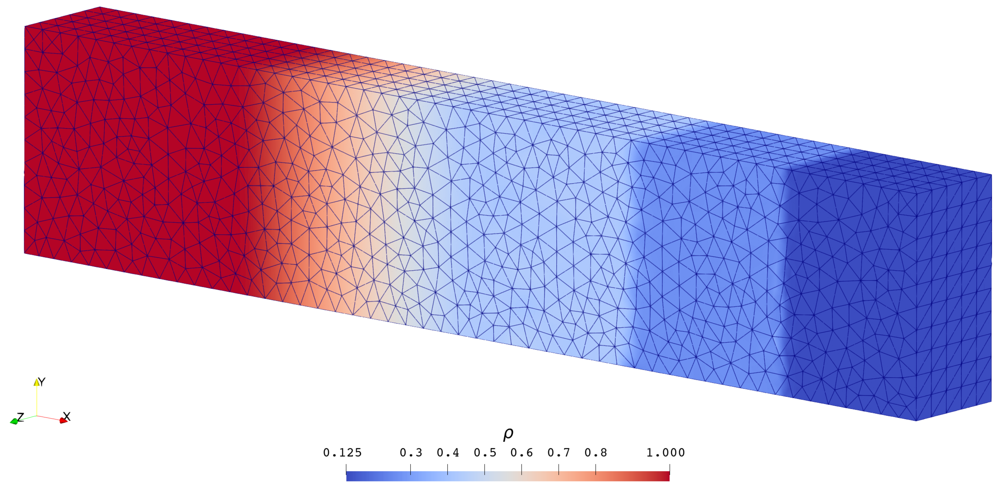
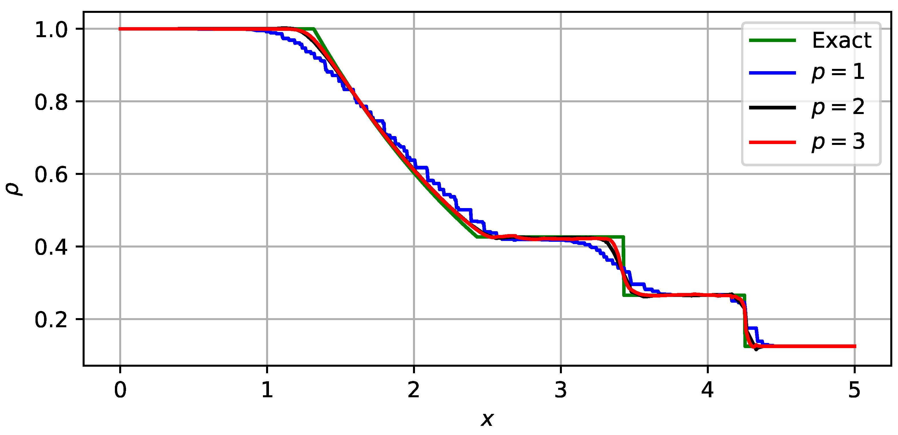
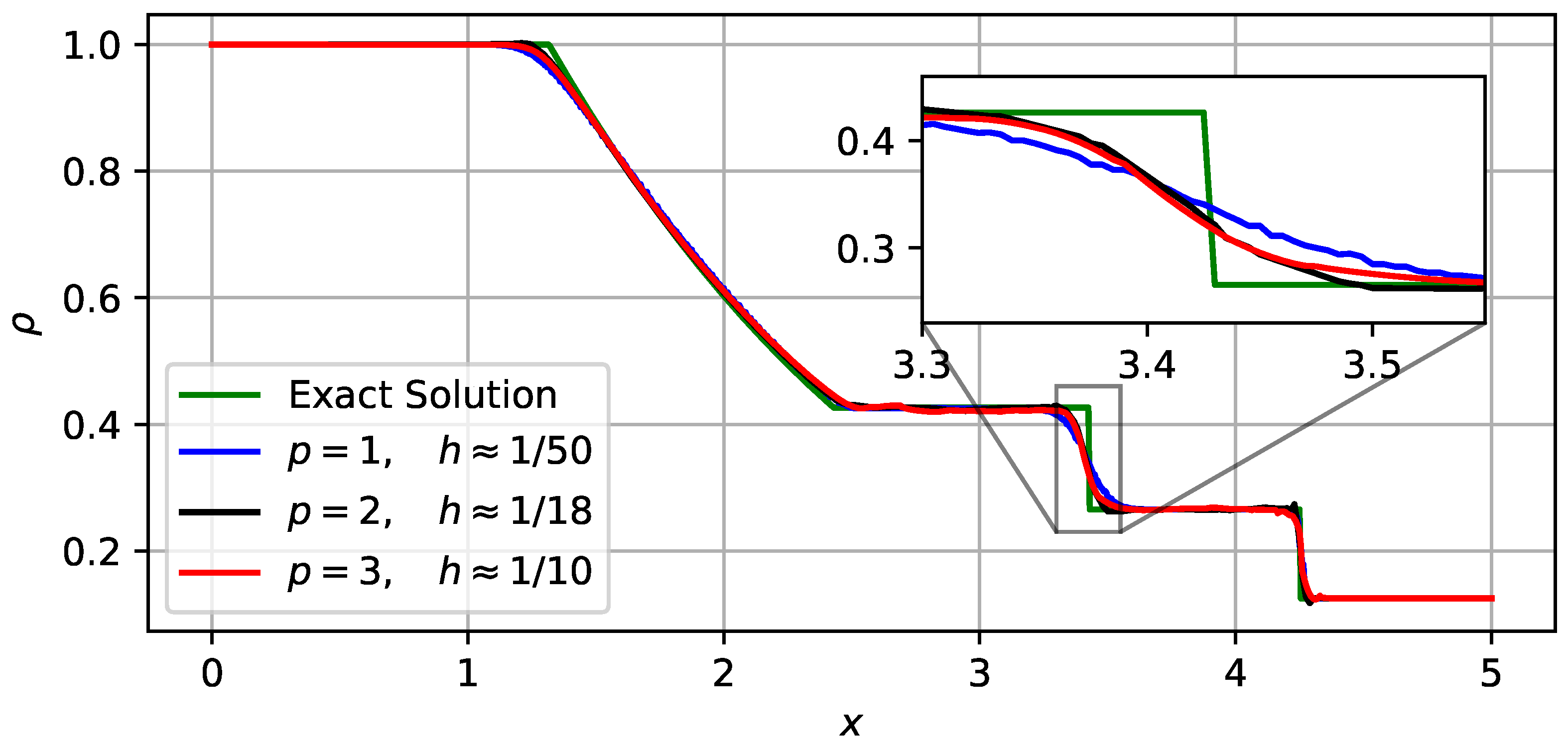
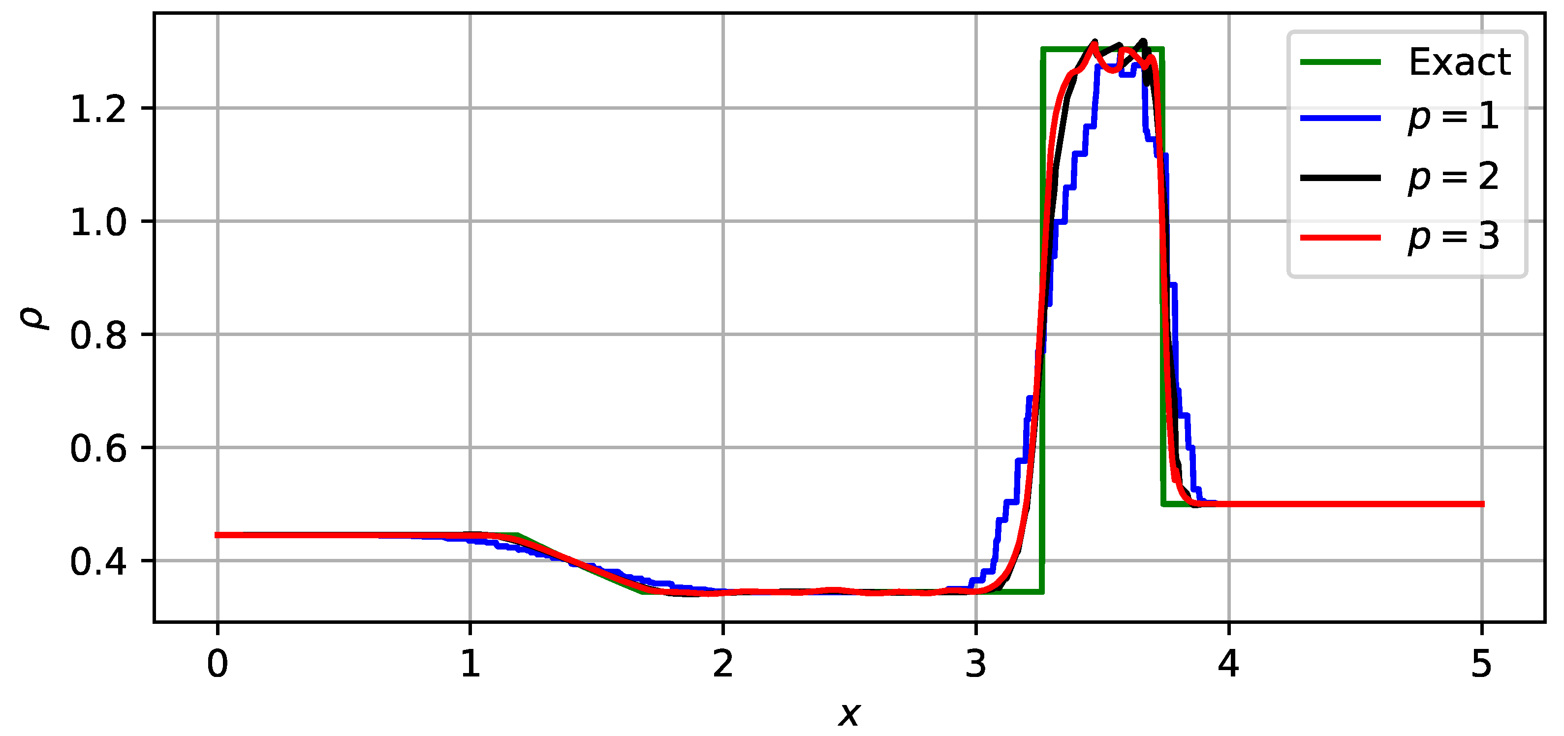
3.1.1. Shock Tube Problems

These problems are usually defined as one-dimensional problems, but we treat them as three-dimensional ones. All these problems are considered in a $[0.0,5.0]\times [0.0,1.0]\times [0.0,0.5]$ box with all boundaries closed but the left and right ends open. Using the method described in [27], their exact solutions can be obtained, which can be used for assessing the accuracy of our solvers. In our earlier work [19], we have given the results obtained by running our solvers on an unstructured hexahedral mesh. This time, we use an unstructured tetrahedral mesh instead.

Problem 1

(Sod). Solve the Euler system Equation (1) for $t\in [0.0,1.0]$ with the initial condition

$${\left[\begin{array}{ccccc}\rho & u& v& w& p\end{array}\right]}_{t=0}=\left\{\begin{array}{cc}\left[\begin{array}{ccccc}1& 0& 0& 0& 1\end{array}\right],\hfill & x<2.5;\hfill \\ \left[\begin{array}{ccccc}\frac{1}{8}& 0& 0& 0& \frac{1}{10}\end{array}\right],\hfill & x>2.5.\hfill \end{array}\right.$$

This is a classical problem of inviscid compressible flows. It contains all three types of discontinuities: a shock wave and a contact discontinuity running towards the right and an expansion wave running towards the left. In Figure 1, we plot the density contour given by our third-order solver with an EigenWeno limiter. In Figure 2, we compare the density distributions given by various solvers along the longitudinal axis (on which $y=0.5$ and $z=0.25$) of the box. The accuracy of our solvers and the effect of p-refinement are clear in these figures.

It is predictable that both mesh refinement (decreasing h) and order increment (increasing p) can help to improve accuracy. To compare the performance of solvers with different orders more fairly, it is better to use finer meshes for running lower-order solvers. After a few trials, we find that the solutions given by the h-p pairs listed in

Table 1. Comparison between time costs and file sizes of various h–p pairs.

h	p	#Cells	#Steps	Time Cost	File Size
1/50	1	2,469,675	1500	1492.16 s	1.23 GB
1/18	2	117045	500	279.119 s	213 MB
1/10	3	19,815	250	201.034 s	89.1 MB

roughly have the same level of accuracy, as shown in Figure 3. It is clear, at least for Problem 1, that high-order solvers are better than low-order ones in the sense of obtaining the same level of accuracy with less time and space costs. Similar conclusions were drawn in our previous work [19], in which the $p=3$ solution of a linear advection problem on an $h\approx 1/4$ mesh defeated the $p=1$ solution of the same problem on an $h\approx 1/32$ mesh in accuracy but saved quite a lot of time. These encouraging results justify our efforts to implement higher-order solvers.

Problem 2

(Lax). Solve the Euler system Equation (1) for $t\in [0.0,0.6]$ with the initial condition

$${\left[\begin{array}{ccccc}\rho & u& v& w& p\end{array}\right]}_{t=0}=\left\{\begin{array}{cc}\left[\begin{array}{ccccc}0.445& 0.698& 0.000& 0.000& 3.528\end{array}\right],\hfill & x<2.5;\hfill \\ \left[\begin{array}{ccccc}0.500& 0.000& 0.000& 0.000& 0.571\end{array}\right],\hfill & x>2.5.\hfill \end{array}\right.$$

This is another problem that involves all three types of discontinuities. It is more difficult than the previous one in the sense that its solution contains values beyond the range of initial values and the discontinuities are much steeper. As before, we plot the density contour of our third-order solution in Figure 4 and compare the density distributions given by various solvers in Figure 5. Both figures demonstrate the effect of p-refinement and the ability of our high-order solvers to suppress numerical oscillations.

Problem 3

(Vacuum). Solve the Euler system Equation (1) for $t\in [0.0,0.4]$ with the initial condition

$${\left[\begin{array}{ccccc}\rho & u& v& w& p\end{array}\right]}_{t=0}=\left\{\begin{array}{cc}\left[\begin{array}{ccccc}1& -4& 0& 0& 0.4\end{array}\right],\hfill & x<2.5;\hfill \\ \left[\begin{array}{ccccc}1& +4& 0& 0& 0.4\end{array}\right],\hfill & x>2.5.\hfill \end{array}\right.$$

This problem is easier than the previous two in the sense that no strong discontinuities (shock or contact discontinuity) occur in the solution. However, there is a region of vacuum, which does not occur in the previous problems, generated between the left- and right-running expansion waves. The velocity u inside the vacuumed region (denoted by a ∗ in subscript) is undefined, but its boundary values should be determined from the left (denoted by an L in subscript) and right (denoted by an R in subscript) initial values by the two Riemann invariants:

$$u_{*L}=u_L+\frac{2a_L}{\gamma -1},u_{*R}=u_R-\frac{2a_R}{\gamma -1}.$$

See [27] for more detailed discussions. Unfortunately, approximate Riemann solvers usually (have to) neglect this condition. For this reason, we use an exact Riemann solver to obtain fluxes on cell boundaries. As before, we plot the results in Figure 6 and Figure 7, which again validate the correctness and robustness of our solvers.

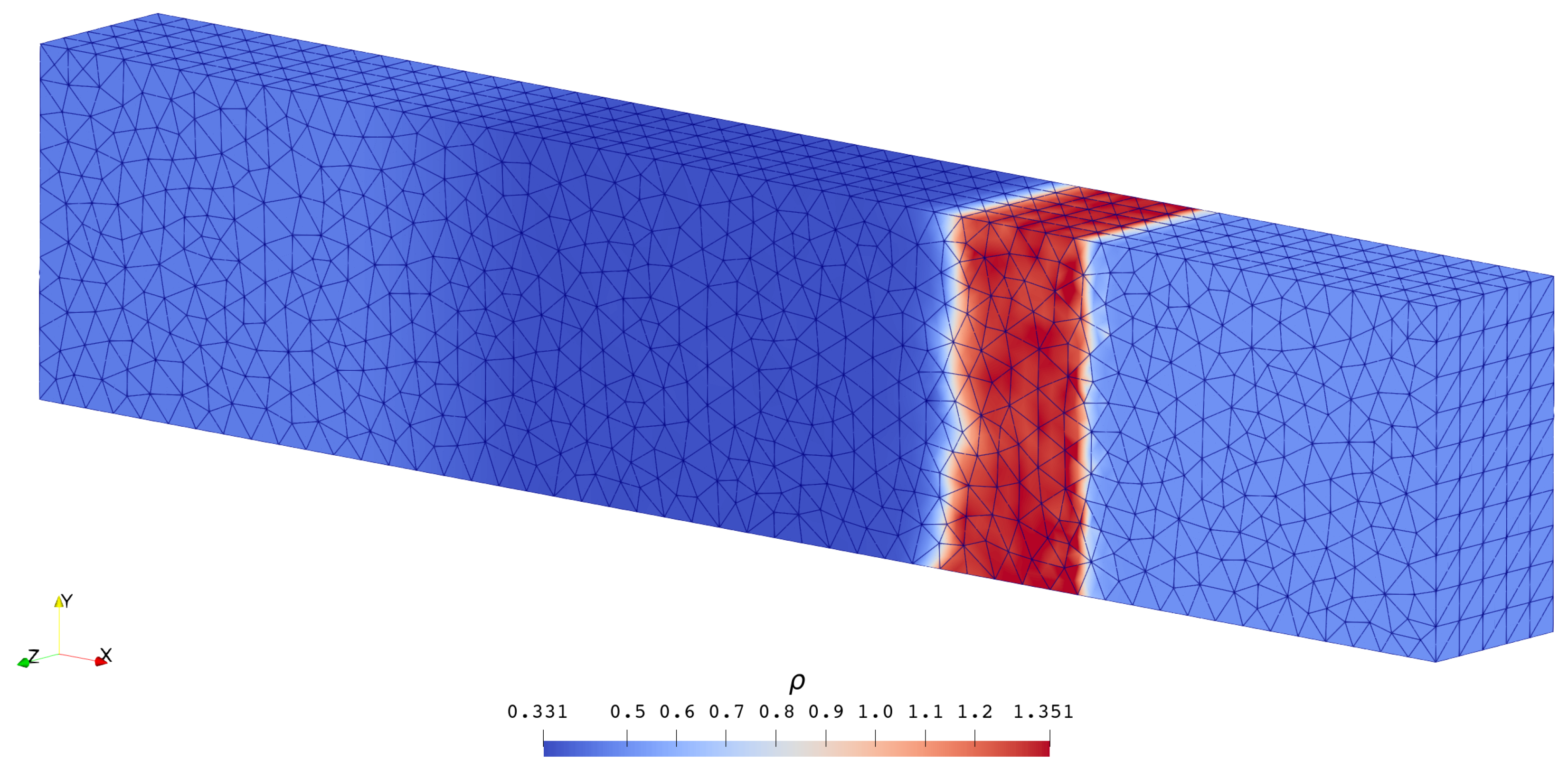
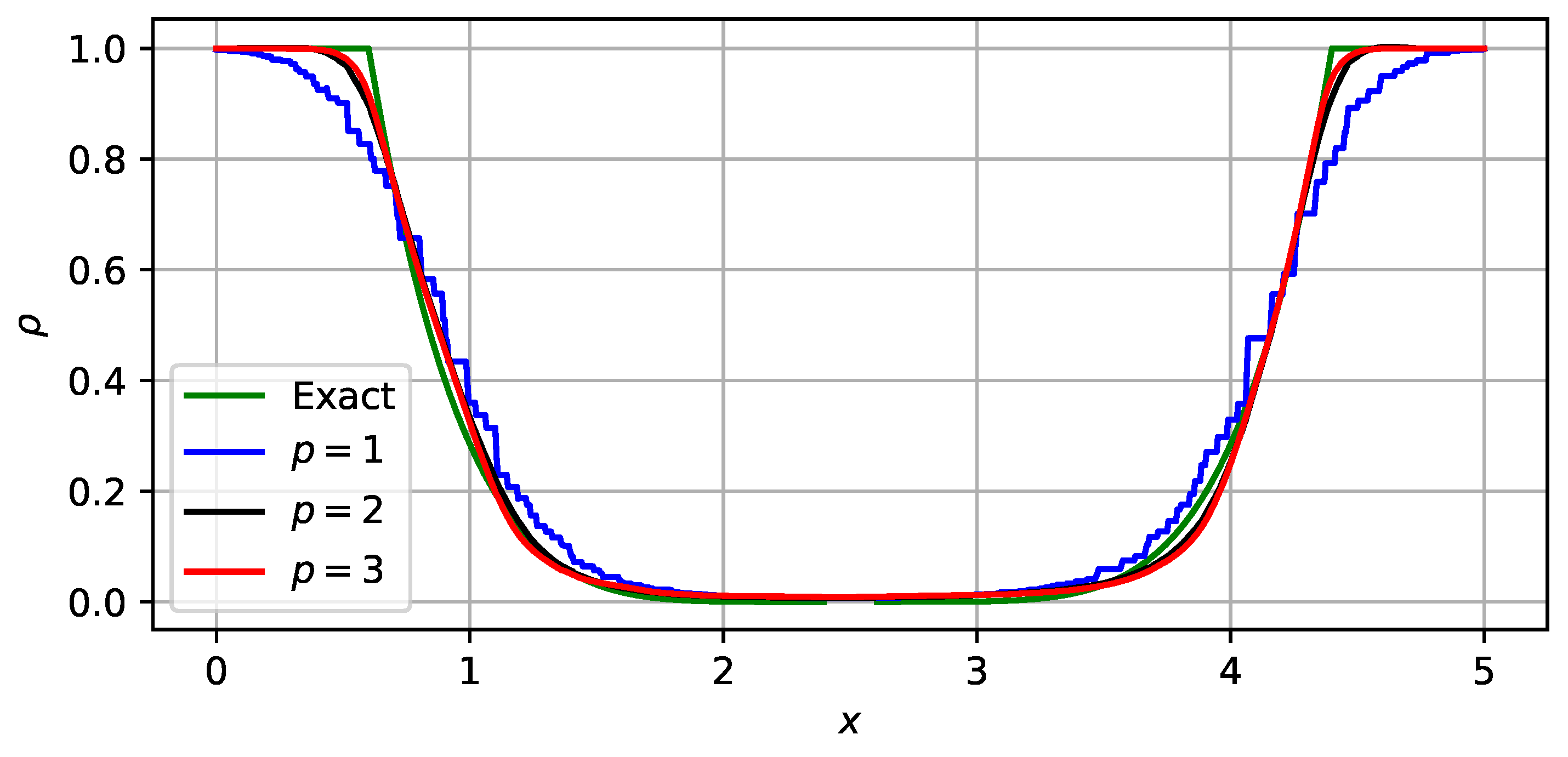
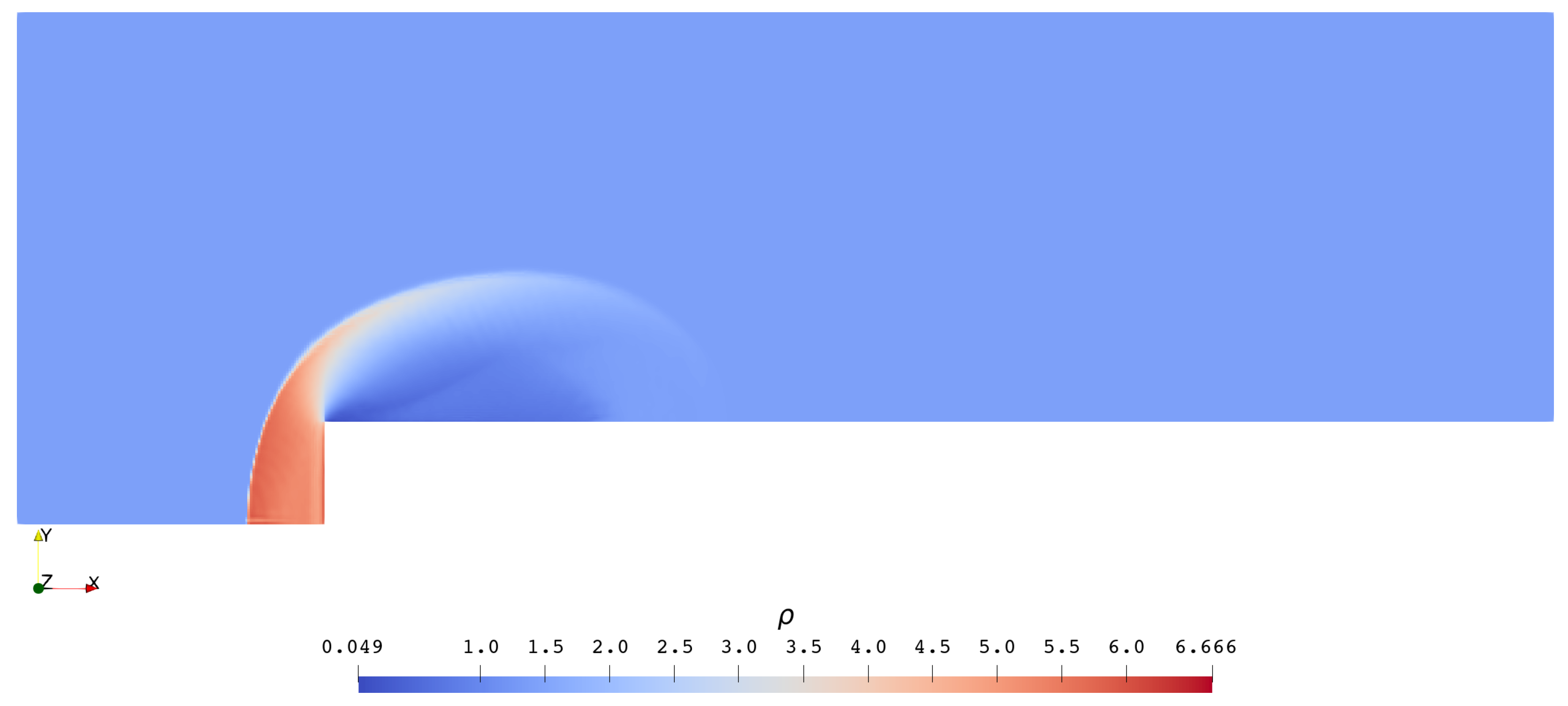
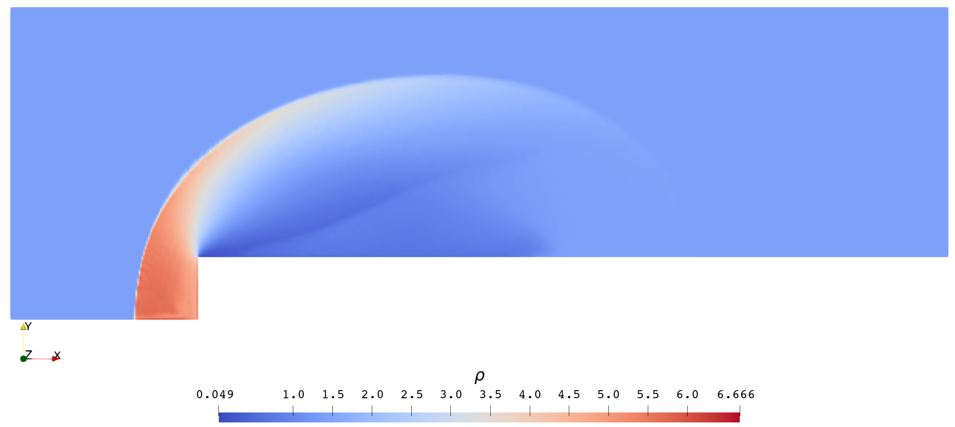
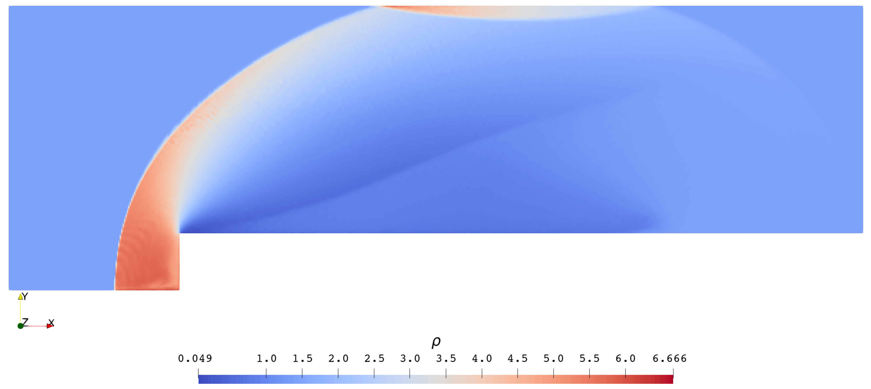
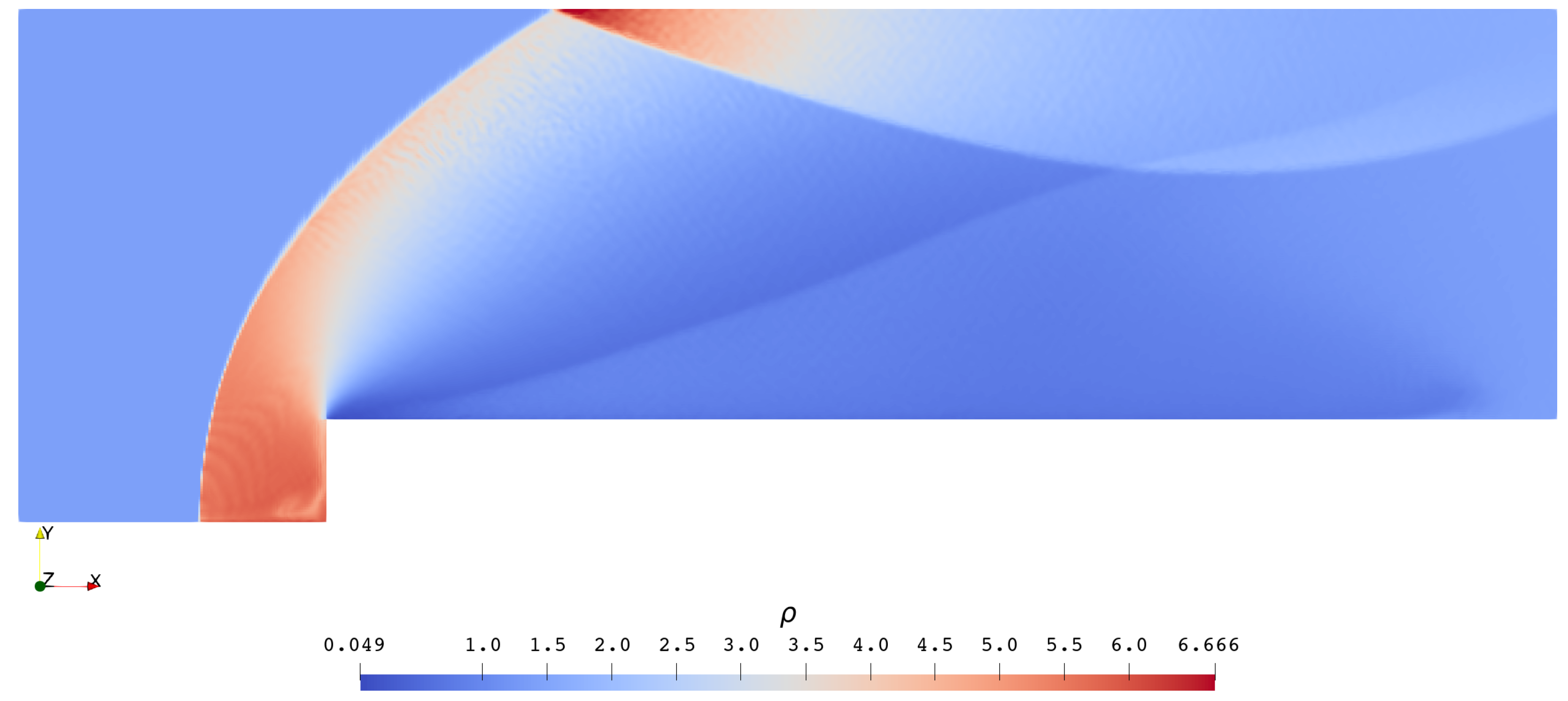
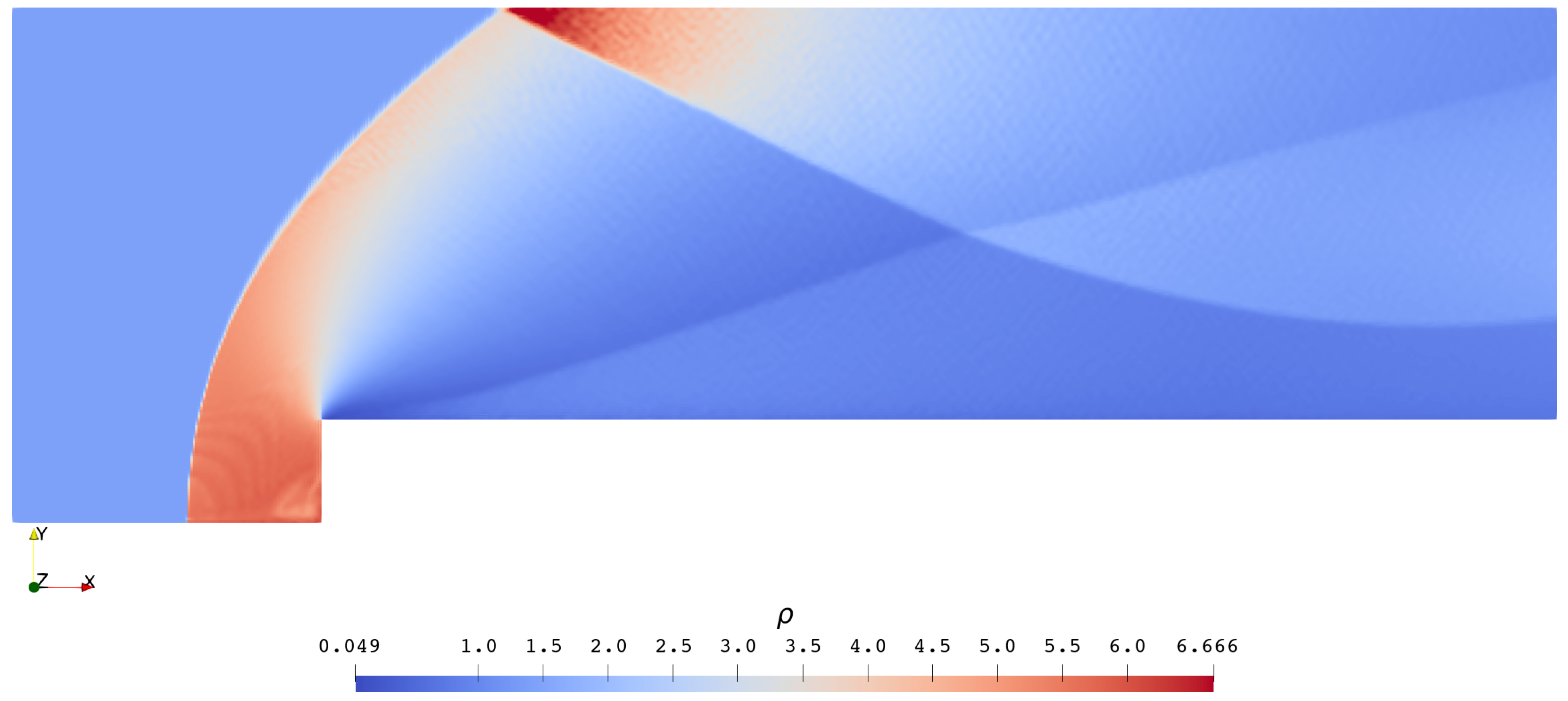
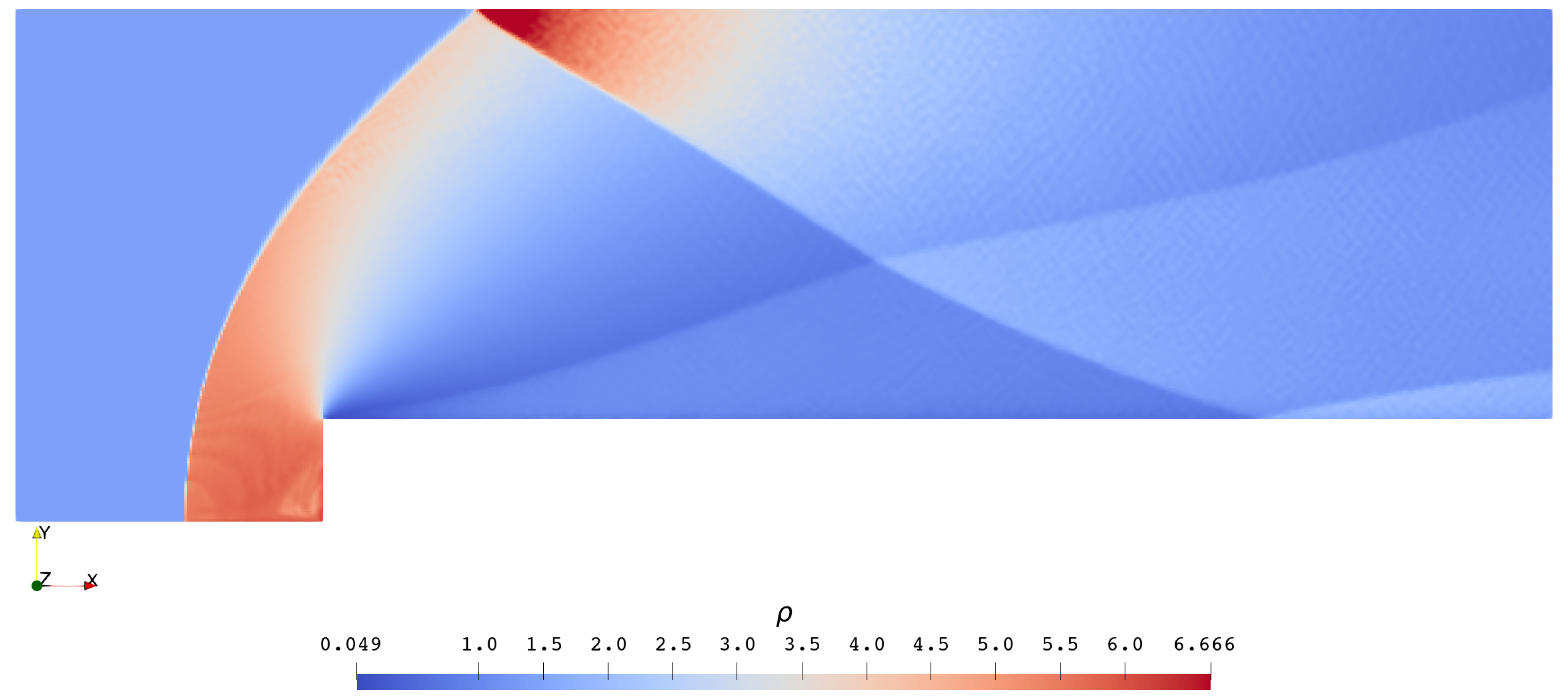
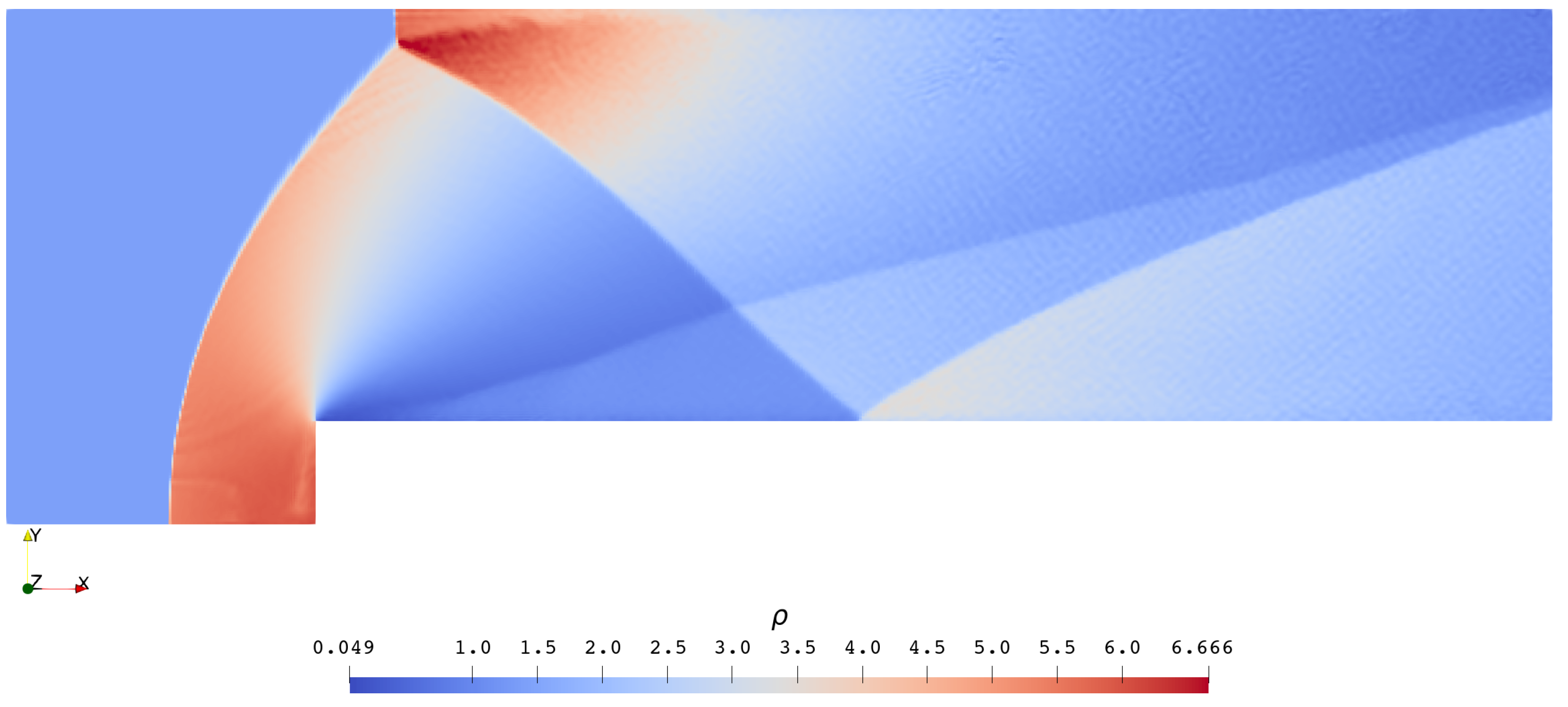
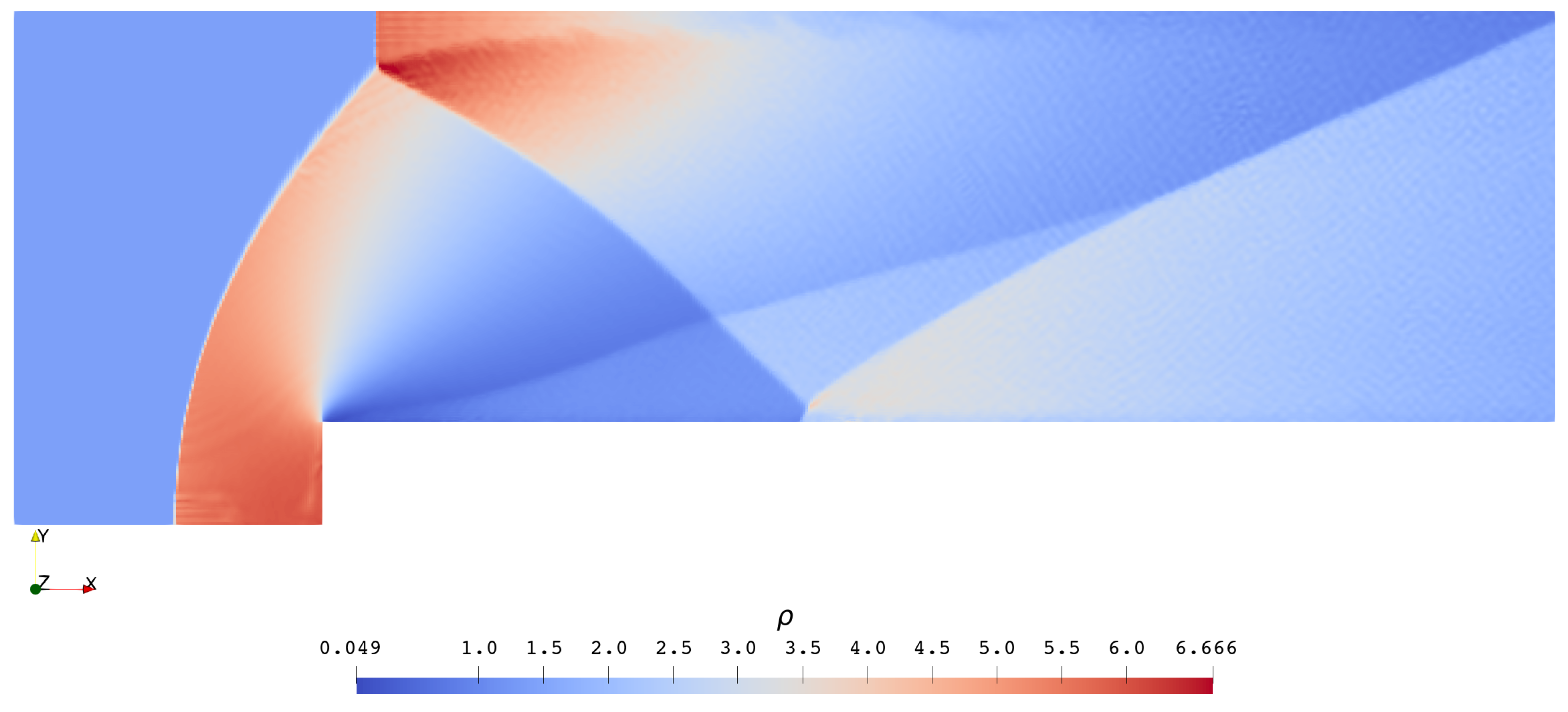
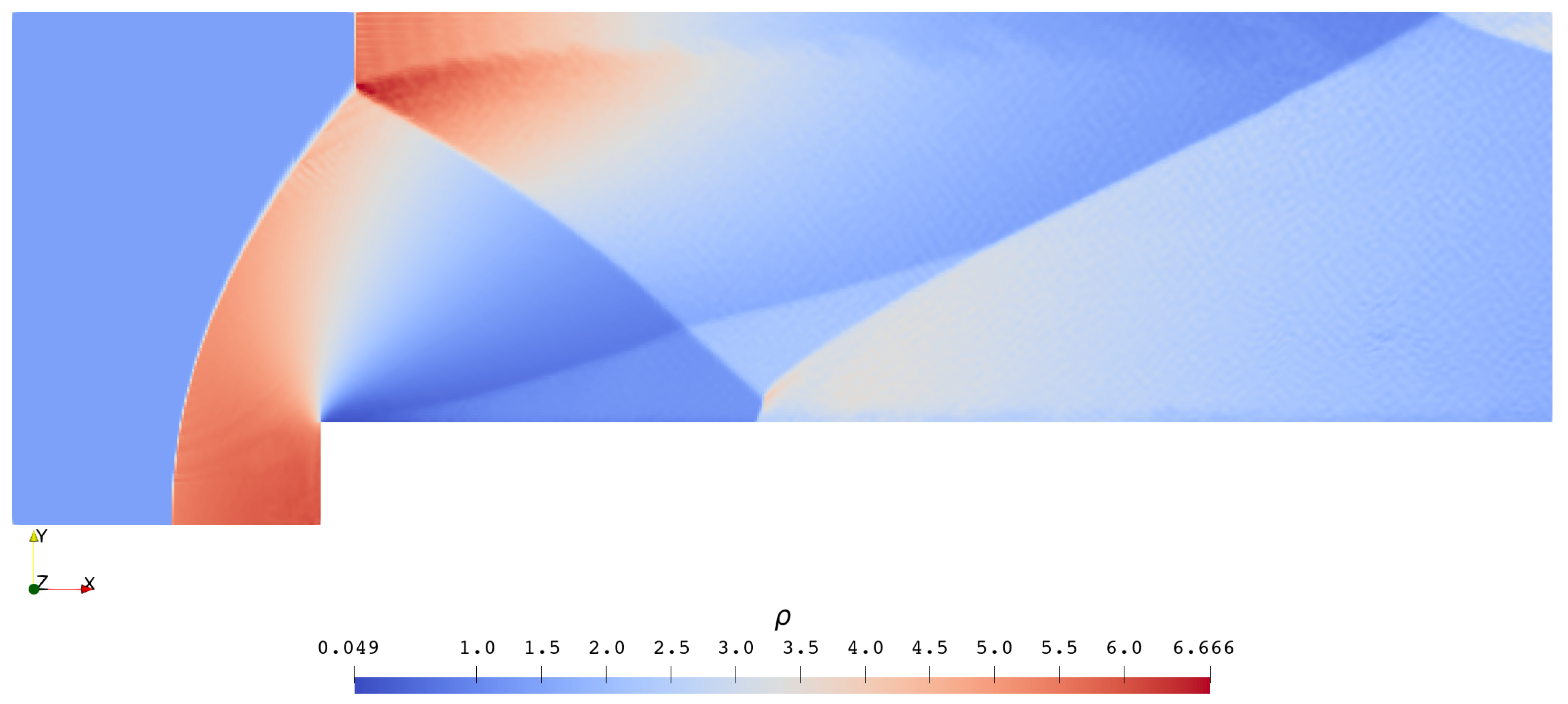
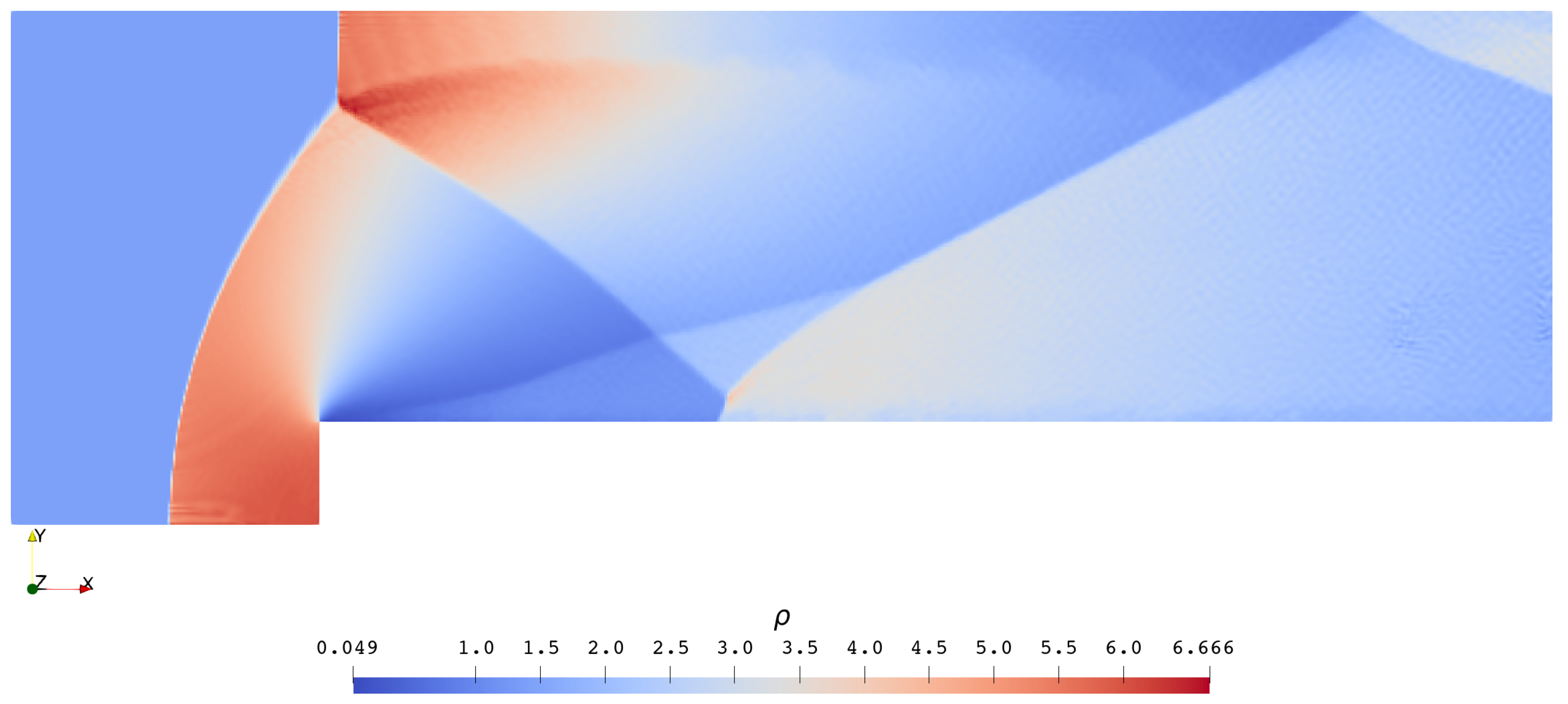
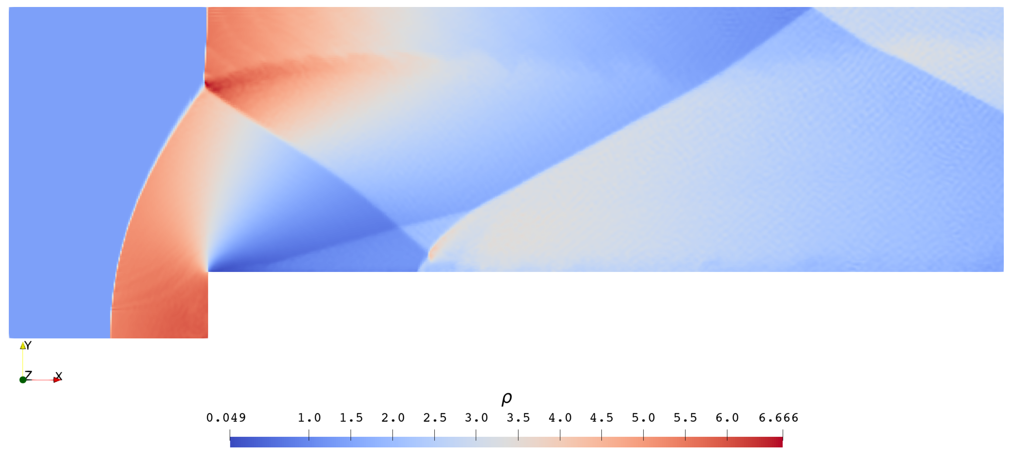
3.1.2. The Forward Step Problem

This is a classical two-dimensional problem [31], but we treat it as a three-dimensional one:

Problem 4.

Solve the Euler system (Equation 1) in a $[0,3]\times [0,1]\times [0,Z]$ box (representing a wind tunnel), where the thickness Z could be any positive value, with a $[0.6,3]\times [0,0.2]\times [0,Z]$ box removed (representing a forward-facing step). The $x=0$ surface is open as an inlet and the $x=3$ surface is open as an outlet. All other boundary surfaces are closed as solid walls. The initial condition is given as a uniform state:

$${\left[\begin{array}{ccccc}\rho & u& v& w& p\end{array}\right]}_{t=0}=\left[\begin{array}{ccccc}1.4& 3.0& 0.0& 0.0& 1.0\end{array}\right].$$

To show the applicability of our solvers on structured meshes, we solve this problem on meshes such as the one in Figure 8. As a common practice, we plot the density contours at various time steps in Figure 9, Figure 10, Figure 11, Figure 12, Figure 13, Figure 14, Figure 15, Figure 16, Figure 17, Figure 18 and Figure 19.

The flow starts from a uniform supersonic ($M=3.0$) state. In Figure 9 and Figure 10, a curved bow shock wave generates in front of the forward-facing step and a fan-shaped expansion wave generates at the corner ($x=0.6,y=0.2$). The bow shock then hits the top of the tunnel (Figure 11) and reflects from it (Figure 12 and Figure 13). At approximately $t=1.2$ (Figure 14), the reflected shock hits the bottom of the tunnel (the top of the step) and reflects from it. Both of the two reflections are regular at these moments. Shortly before $t=2.0$ (Figure 14), a Mach stem that characterizes a Mach reflection is generated from the first reflection point. A wavy contact discontinuity generating from the triple point is captured by Figure 16, Figure 17, Figure 18 and Figure 19. This flow structure would be smeared off if we solved Problem 4 using lower-order solvers or coarser meshes.

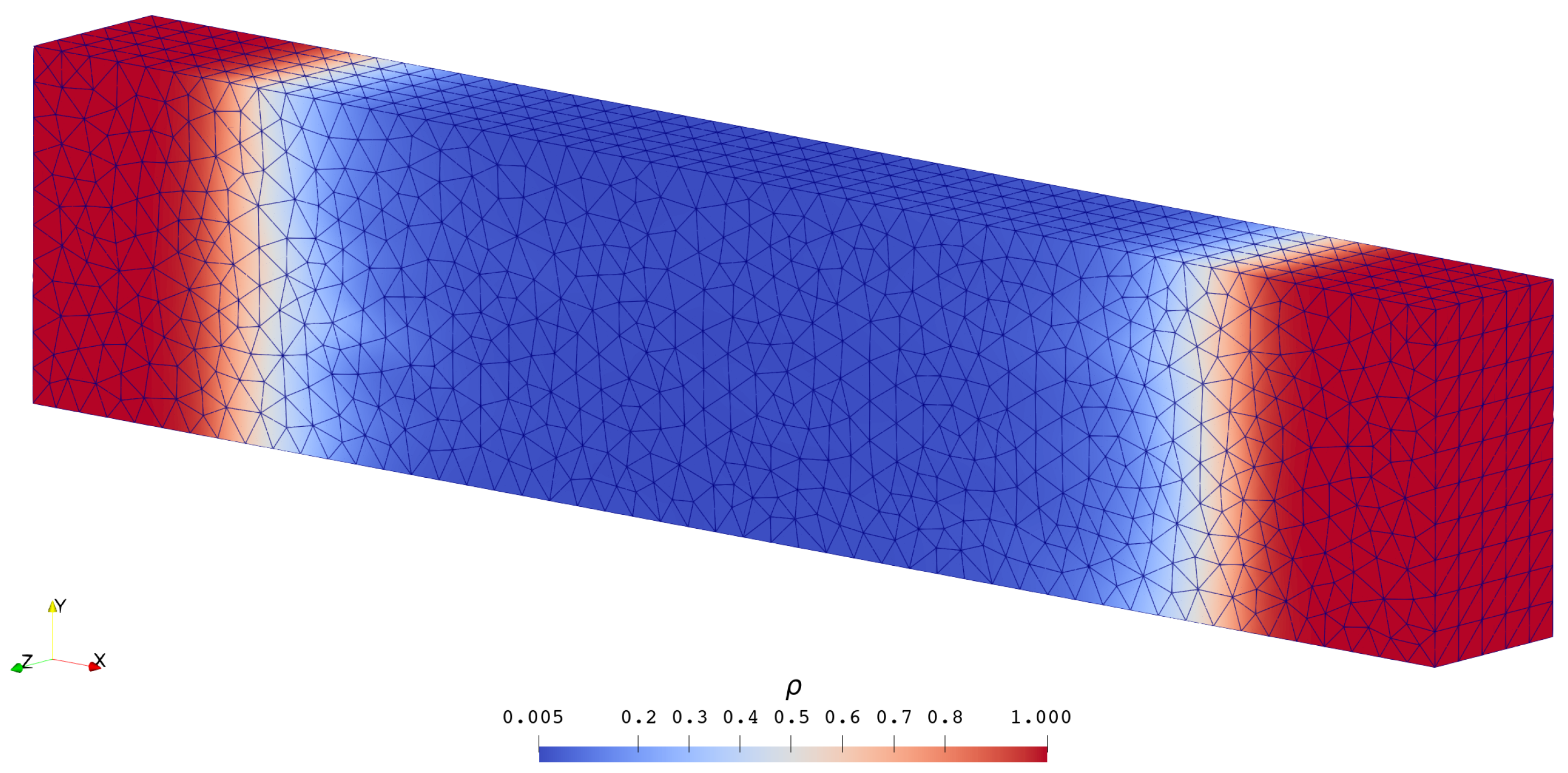
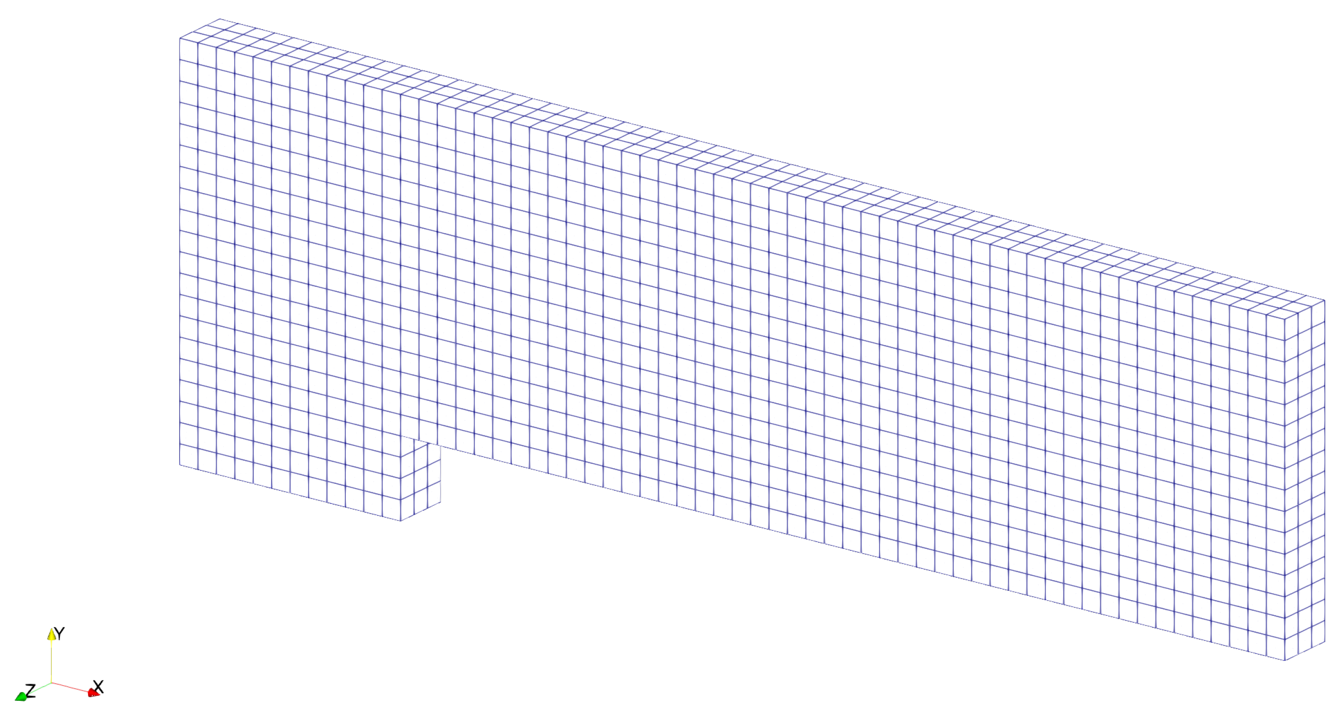
3.2. Three-Dimensional Engineering Problems

In this section, we solve the Euler system Equation (1) on a three-dimensional unstructured mesh, which discretizes the space around a YF-17 aircraft by tetrahedral cells, as shown in Figure 20.

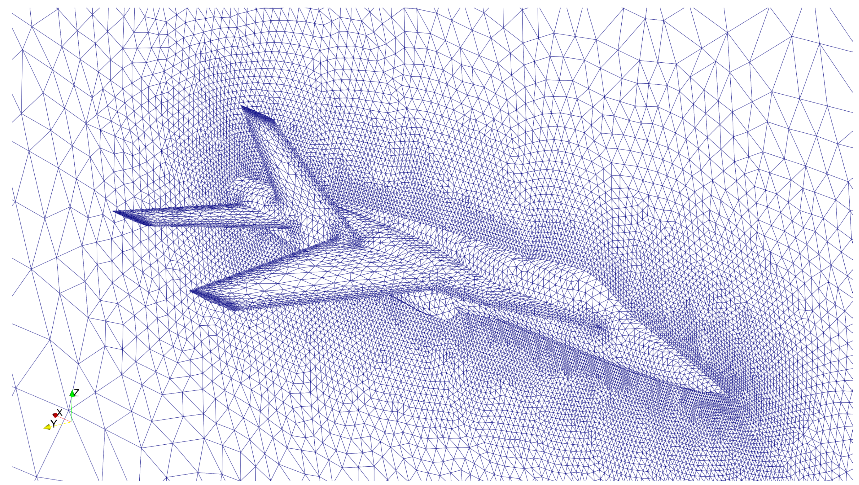
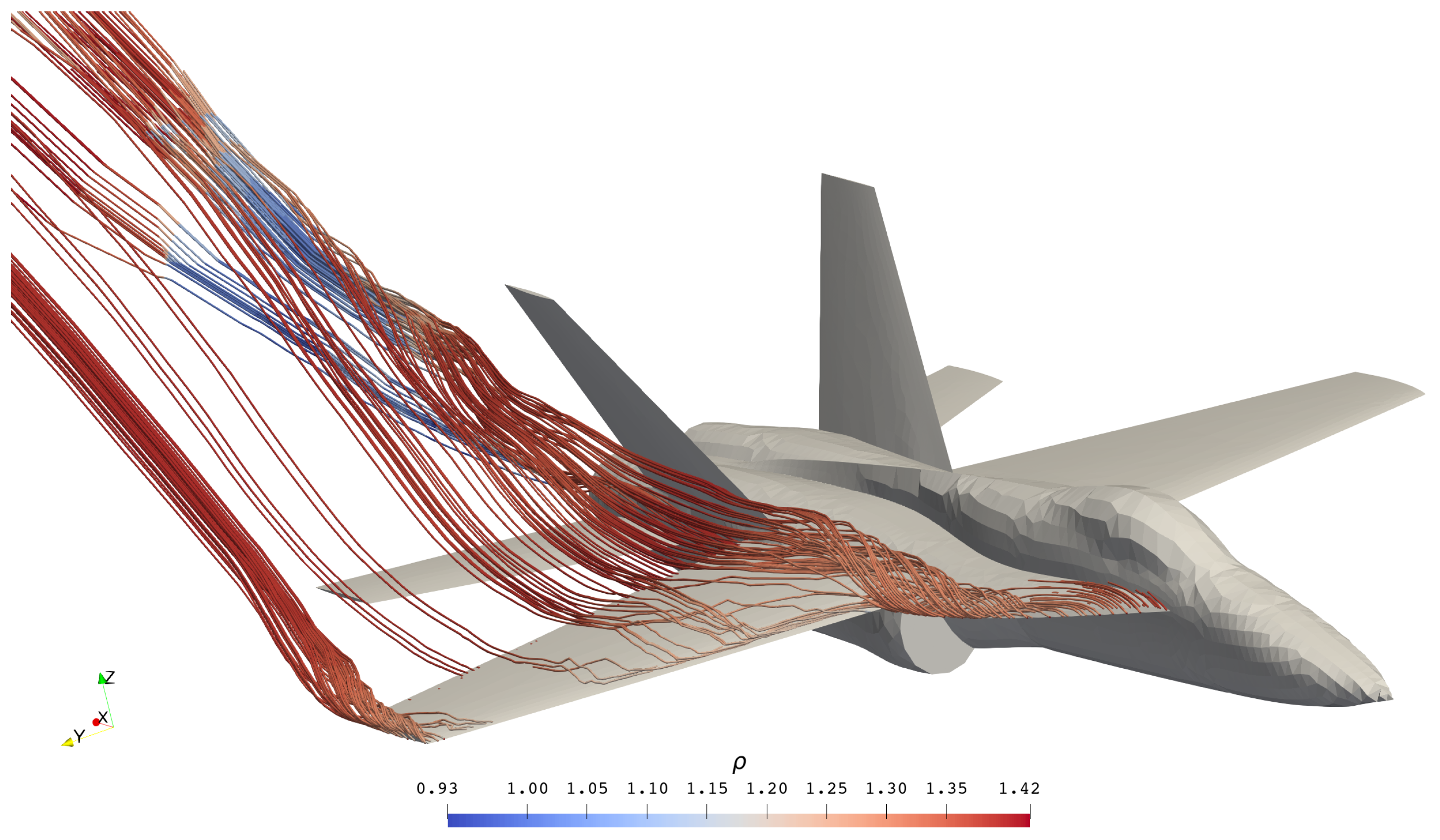
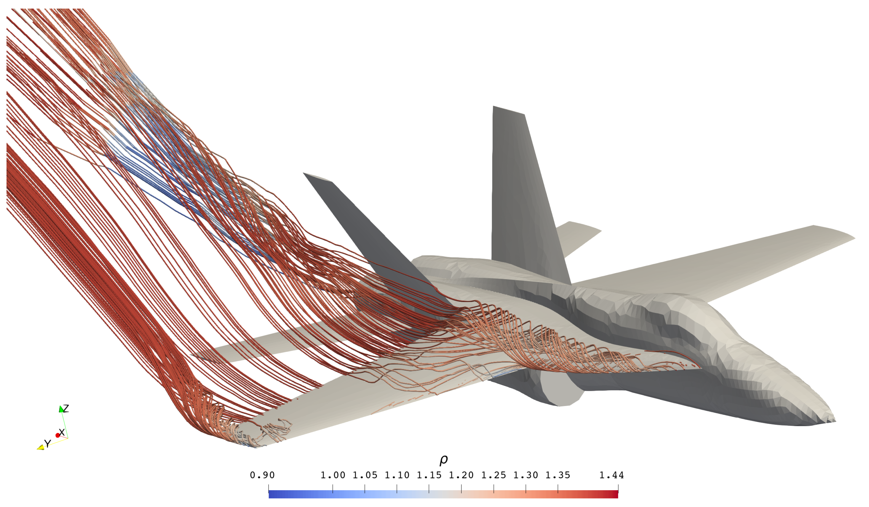
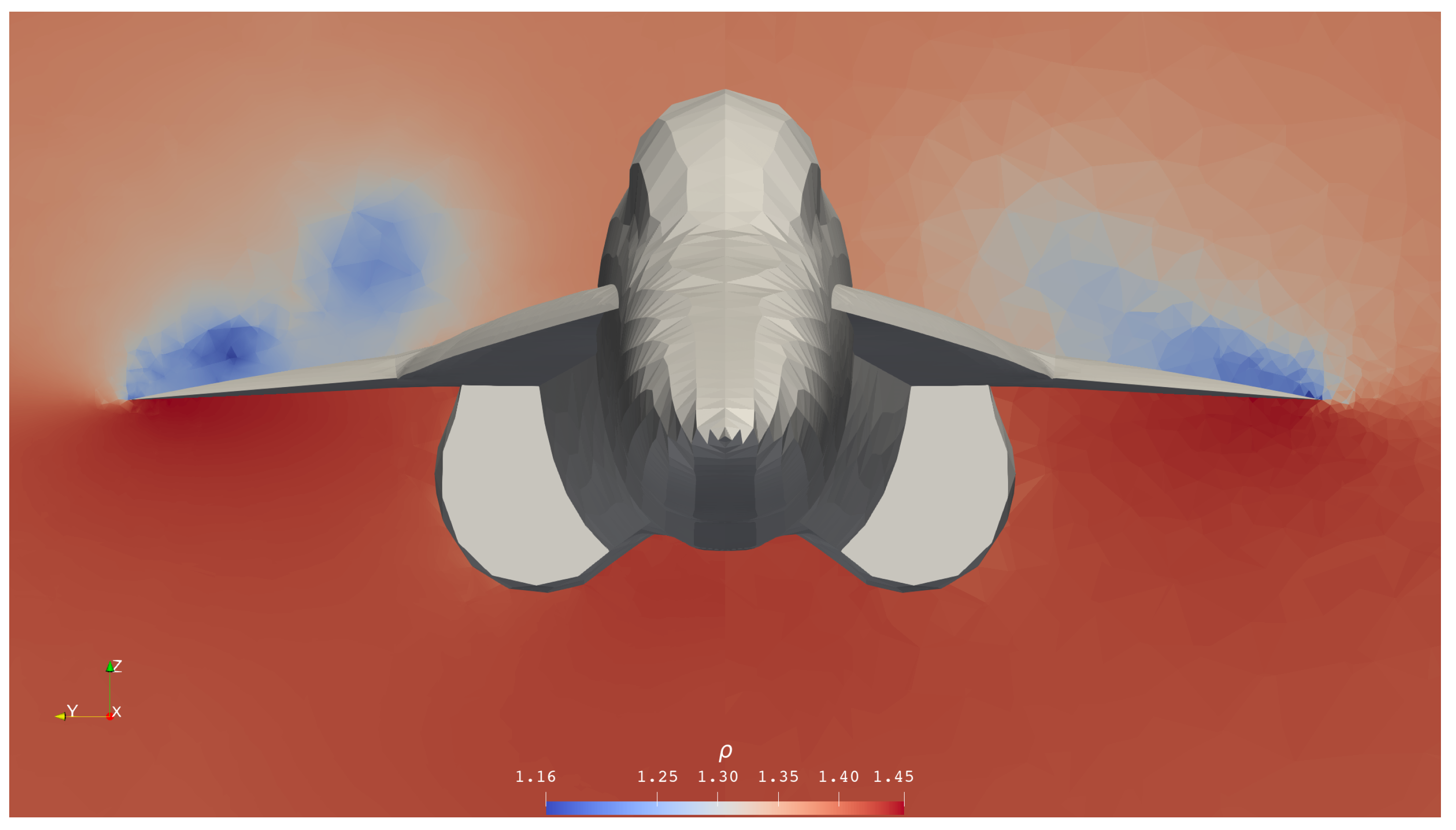
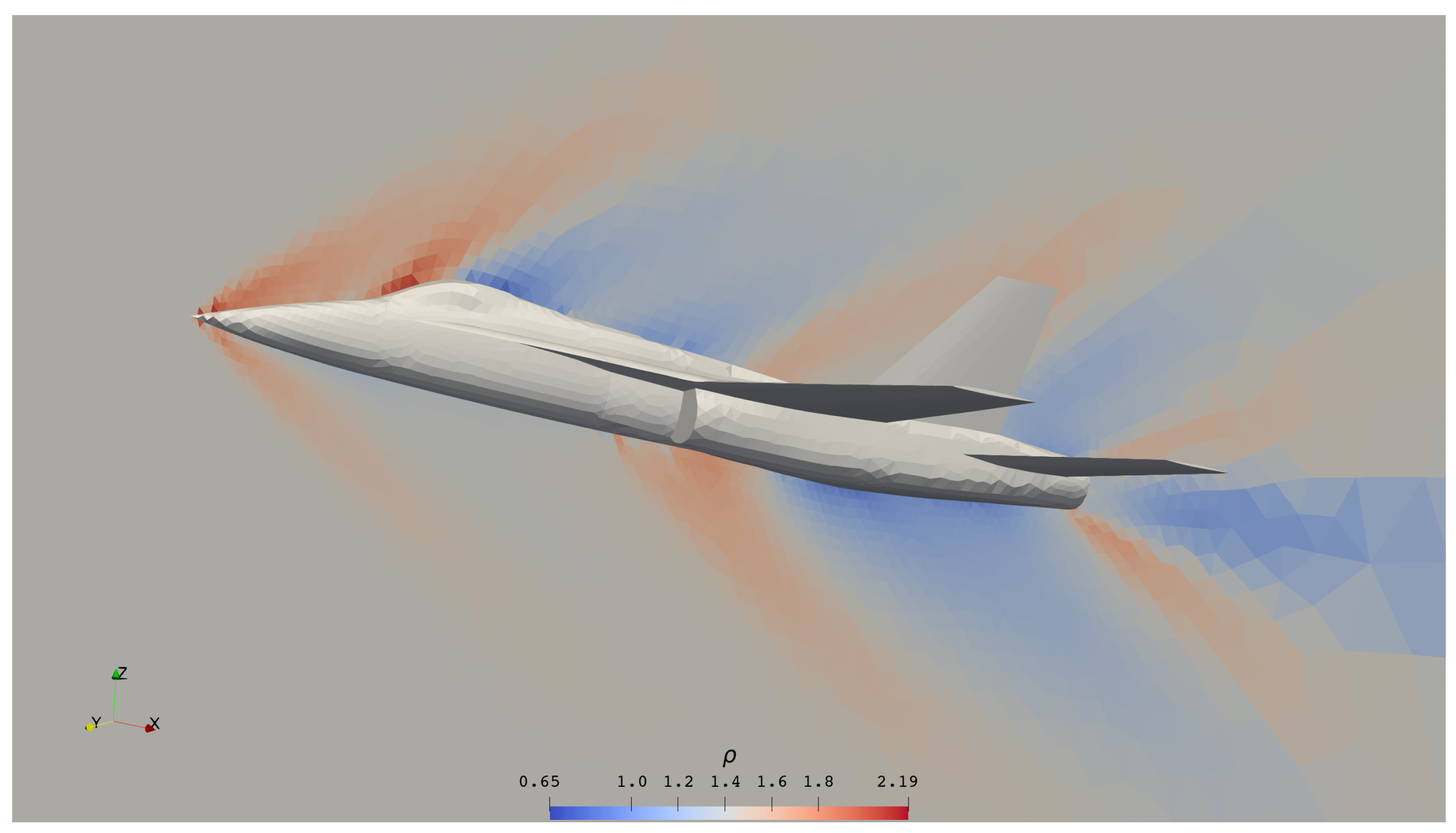
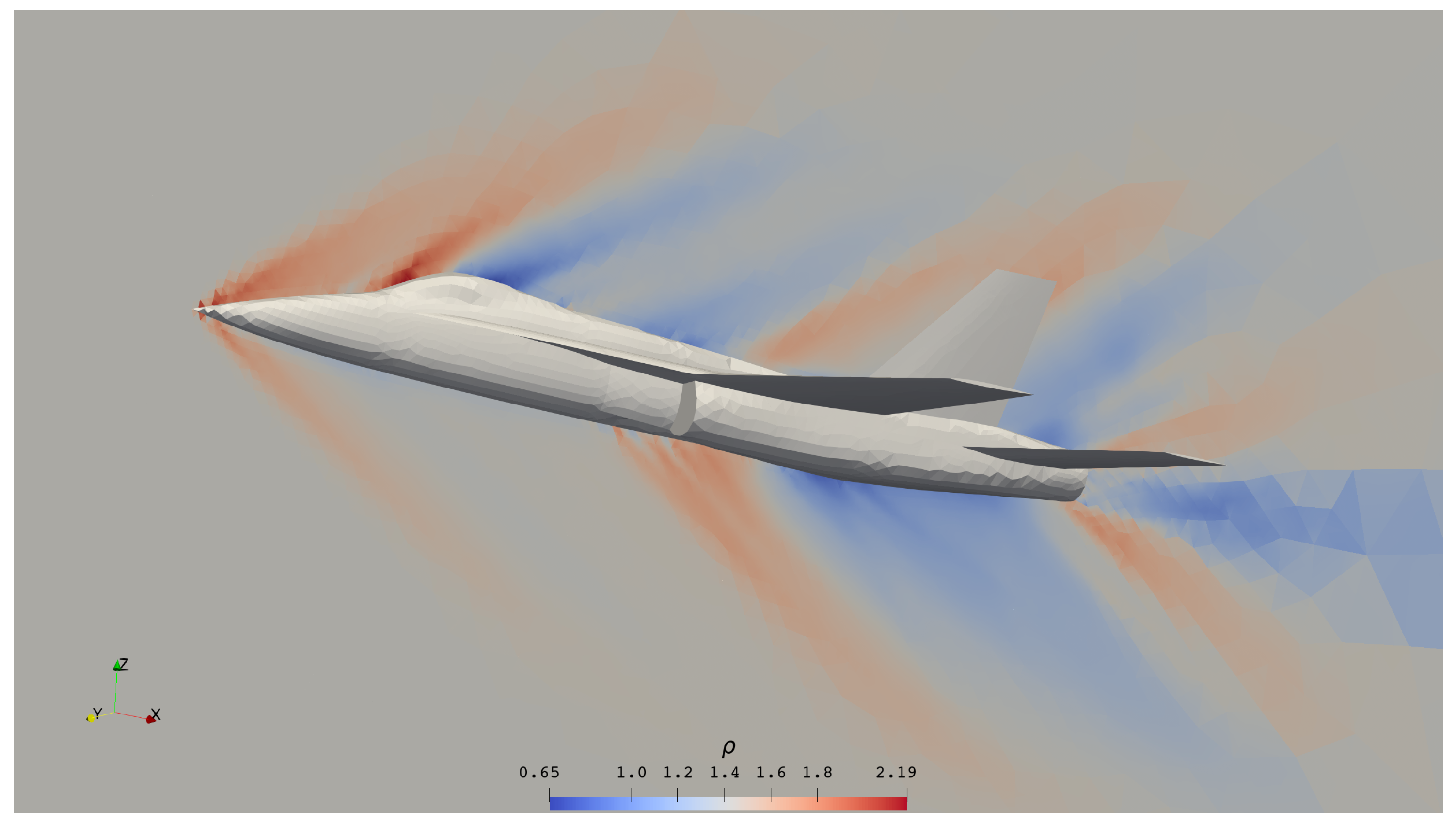
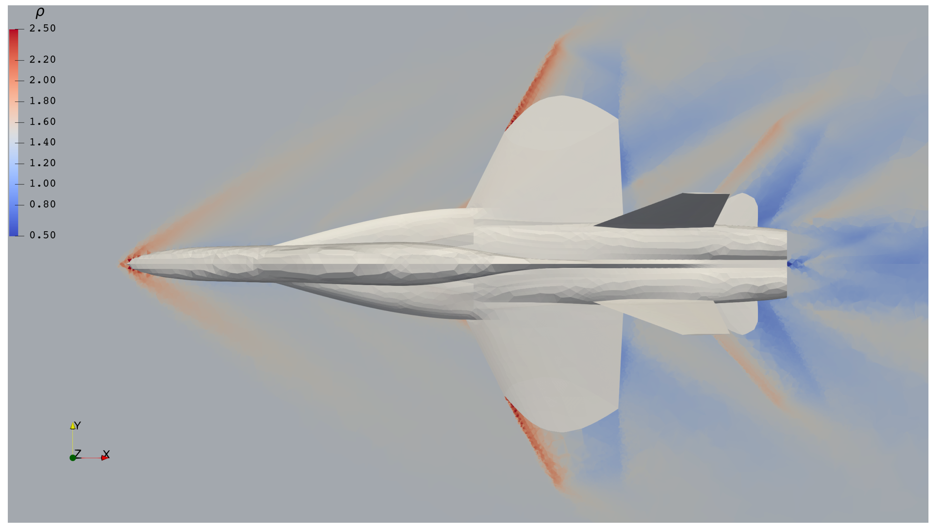
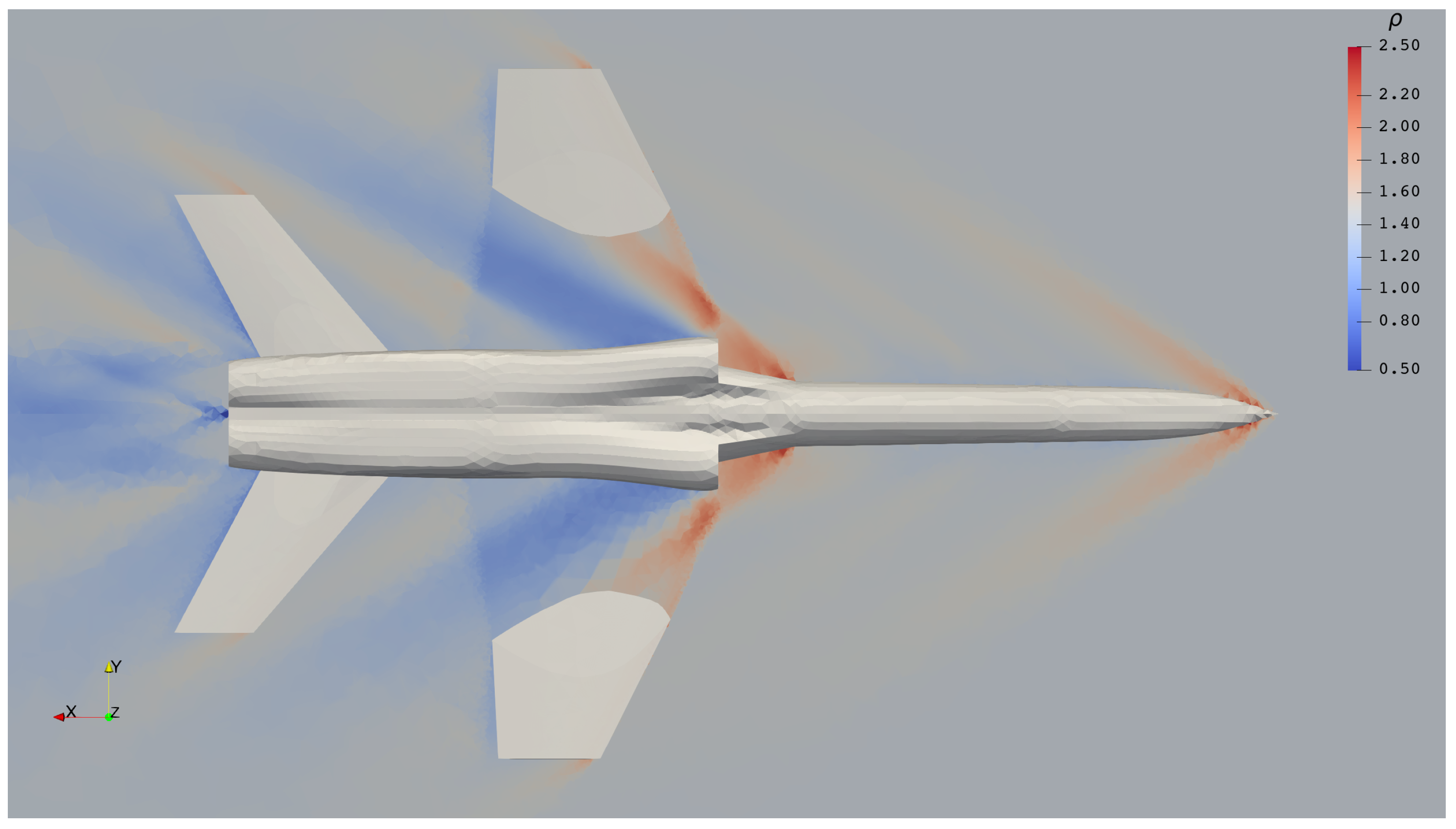
3.2.1. YF-17 in Subsonic Flight

Problem 5.

Solve the Euler system Equation (1) in the surroundings of a YF-17 aircraft. The initial condition is given as a subsonic flow ($M=0.3$) with a 20-deg angle of attack:

$${\left[\begin{array}{ccccc}\rho & u& v& w& p\end{array}\right]}_{t=0}=\left[\begin{array}{ccccc}1.4& 0.2819& 0.0& 0.1026& 1.0\end{array}\right].$$

All boundaries of the aircraft are defined as solid walls, except the intake of the engine, which is defined as a subsonic outlet of the condition equal to the initial condition, and the exhaust of the engine, which is defined as a supersonic ($M=3.0$) inlet of the condition:

$${\left[\begin{array}{ccccc}\rho & u& v& w& p\end{array}\right]}_{\mathrm{ex}.}=\left[\begin{array}{ccccc}1.4& 2.4& 0.0& 0.0& 1.44\end{array}\right].$$

We solve this problem via two of our finite element solvers and plot the streamlines released from the strake and the wing at $t=10$ in Figure 21 and Figure 22. It can be seen that the streamlines obtained from the high-order ($p=3$) solution are smoother than those from the low-order ($p=1$) solution, which shows the benefit of p-refinement. The difference in accuracy is more obvious in Figure 23, which clearly shows a more detailed flow structure in the third-order solution (left half) and the piecewise constantness of the first-order solution (right half). Both solutions are able to capture the vortex trailing from the wing tip, which is generated from the the pressure difference between the upper and lower surfaces of the wing. When the wing generates positive lift, the pressure on the lower wing surface is higher than that on the upper wing surface. Under the action of this pressure difference, the air under the wing rolls up around the tip and flows backward, and the tip vortex is thus formed. The vortex trailing from the strake is generated from a similar mechanism.

3.2.2. YF-17 in Supersonic Flight

Problem 6.

Solve the Euler system Equation (1) in the surroundings of a YF-17 aircraft. The initial condition is given as a supersonic flow ($M=2.0$) with a 0-deg angle of attack:

$${\left[\begin{array}{ccccc}\rho & u& v& w& p\end{array}\right]}_{t=0}=\left[\begin{array}{ccccc}1.4& 2.0& 0.0& 0.0& 1.0\end{array}\right].$$

All boundaries of the aircraft are defined as solid walls, except the intake of the engine, which is defined as a supersonic outlet of the condition equal to the initial condition, and the exhaust of the engine, which is defined as a supersonic ($M=3.0$) inlet of the condition:

$${\left[\begin{array}{ccccc}\rho & u& v& w& p\end{array}\right]}_{\mathrm{ex}.}=\left[\begin{array}{ccccc}1.4& 2.4& 0.0& 0.0& 1.44\end{array}\right].$$

We solve this problem using the same solvers as for Problem 5. Density contours on the $y=0$ surface obtained from the first- and the third-order solutions are given in Figure 24 and Figure 25, respectively. It is obvious that shock waves are captured well (without spurious oscillations) by both of them. To show the difference more clearly, we compare the two solutions in Figure 26 and Figure 27. As in the subsonic case, the third-order solution (which is piecewise quadratic) outperforms the first-order one (which is piecewise constant). Shock waves (red) are generated on surfaces facing the wind, since the relative speed of air is larger than the speed of sound. Expansion waves (blue) are generated on leeward surfaces, since the solid body contracts there, which leaves more room for the supersonic flow.

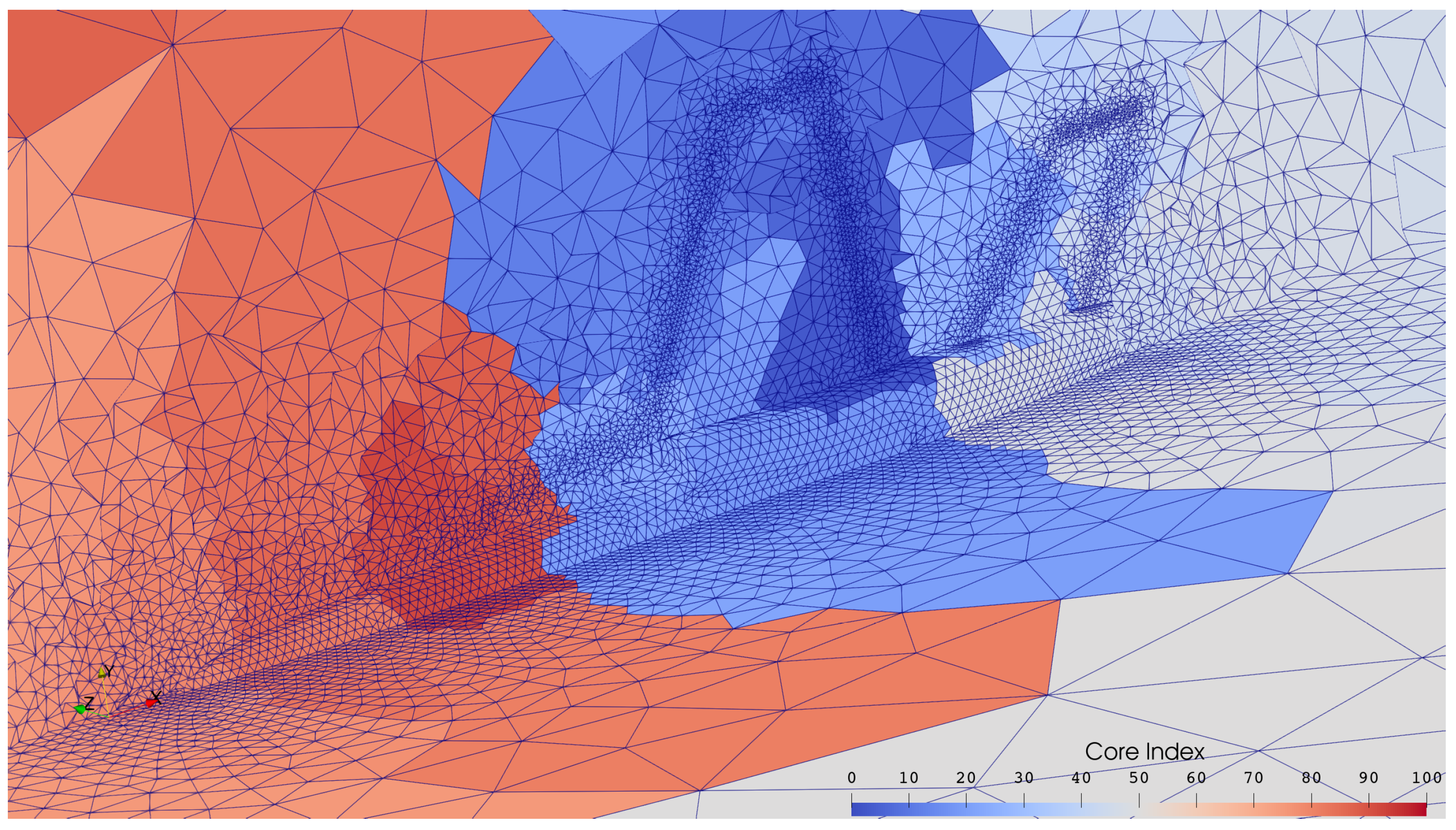
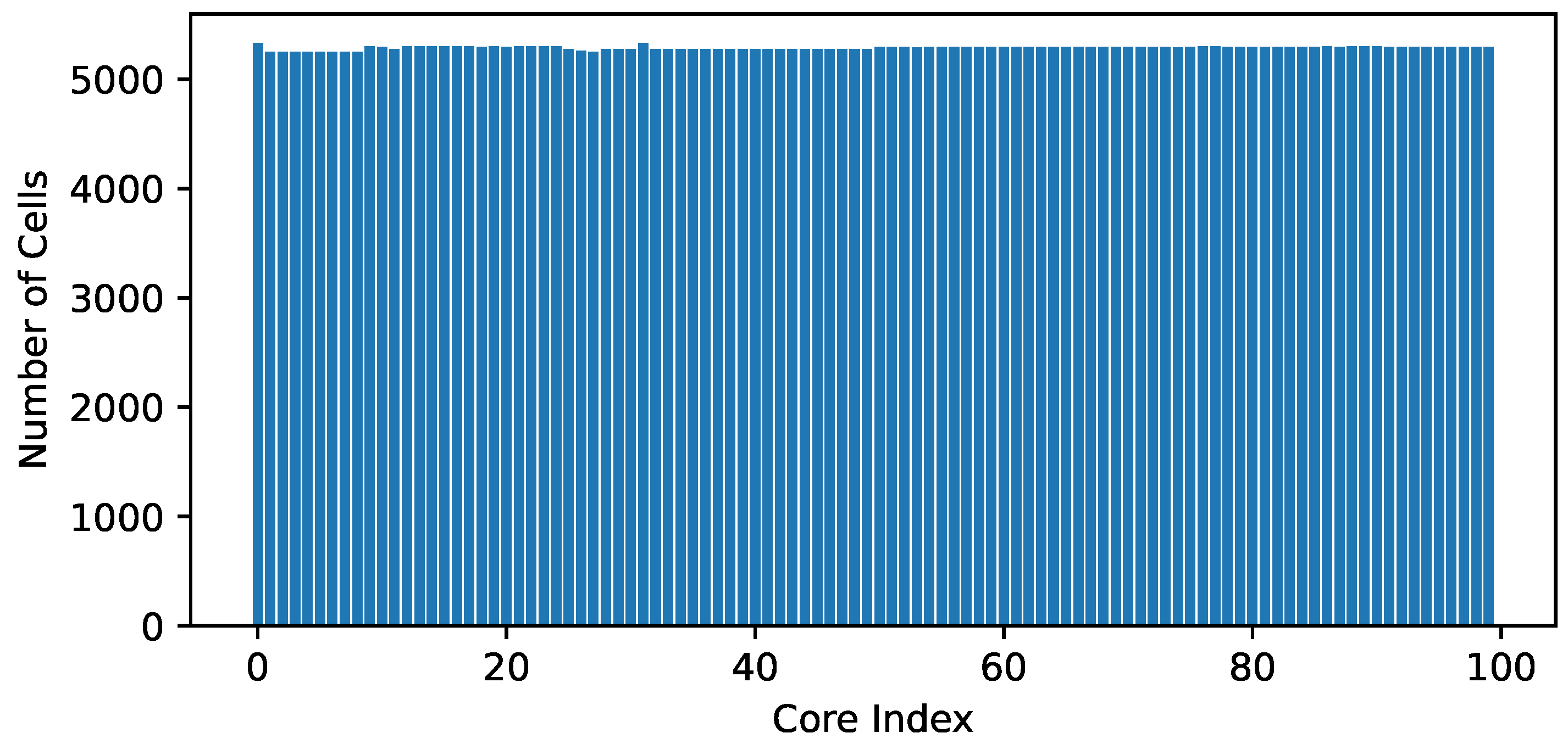
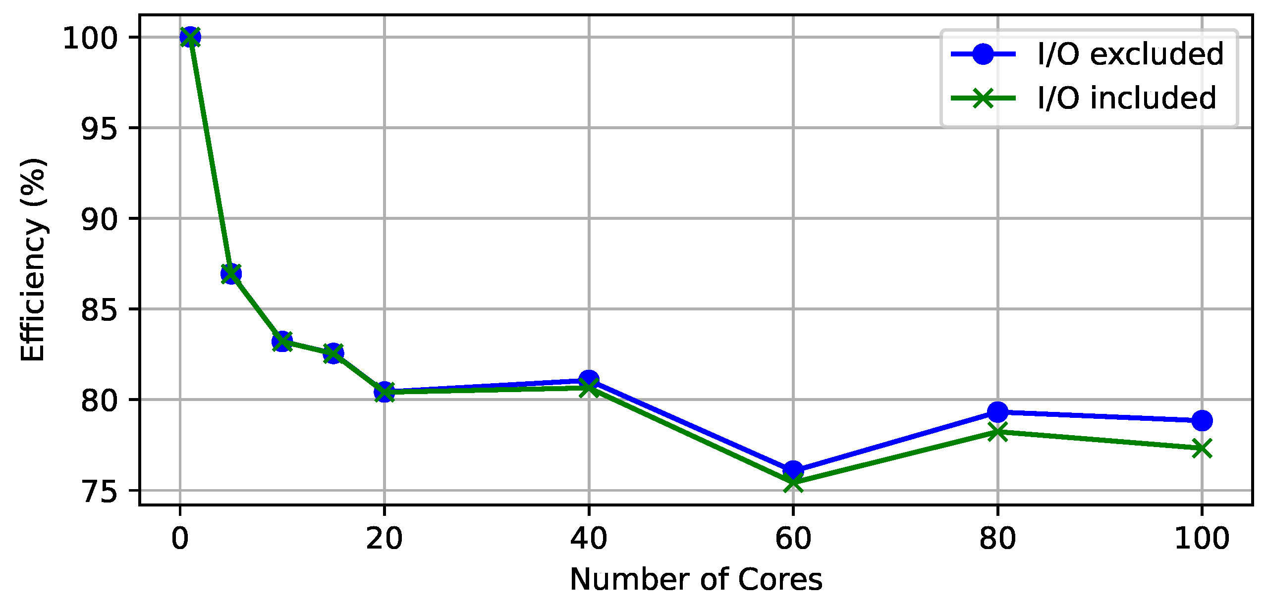
3.2.3. Parallel Efficiency

Since the mesh in Figure 20 is highly unstructured and non-uniform, simple geometric partitioning cannot achieve a relatively balanced distribution of computational effort. In our code, we use the Metis library [32] to partition the dual graph of the mesh, which gives the results in Figure 28 and Figure 29. The fluctuation of cell numbers is under $2\%$, which is quite good since the optimal partitioning of an unstructured mesh is an NP-hard problem. With such an approximately optimal partitioning, the parallel efficiency, which is defined as

$$E=\frac{T_{\mathrm{serial}}}{P{T}_{\mathrm{parallel}}}\times 100\%,$$

in which P is the number of processes, could surpass $99\%$ in theory. In practice, however, the E values given by our numerical experiments are only around $80\%$, as shown in Figure 30, which is derived from the measured time costs given in

Table 2. Time costs of the third-order solver running on different numbers of cores.

P	${\mathit{T}}_{100}$	${\mathit{T}}_{399}$	${\mathit{T}}_{400}$	$\mathit{P}\frac{{\mathit{T}}_{399}-{\mathit{T}}_{100}}{399-100}$	$\mathit{P}\frac{{\mathit{T}}_{400}-{\mathit{T}}_{100}}{400-100}$
1	10,511.3	42,466.5	42,593.0	106.873	106.939
5	2389.25	9740.13	9769.96	122.925	123.012
10	1246.37	5086.62	5101.95	128.436	128.519
15	839.554	3420.17	3430.75	129.462	129.560
20	645.737	2632.32	2640.57	132.882	132.989
40	325.269	1310.72	1319.73	131.833	132.595
60	222.890	923.043	931.754	140.499	141.773
80	168.862	672.439	681.445	134.736	136.689
100	137.787	543.081	552.682	135.550	138.298

. The main reason for the gap between theory and practice is that in the derivation of the ideal E value, inter-process communications are assumed to overlap in time with inner-cell computations, which is an over-optimistic assumption. Nevertheless, the acceleration is still significant, which reduces the wall clock time to an acceptable level.

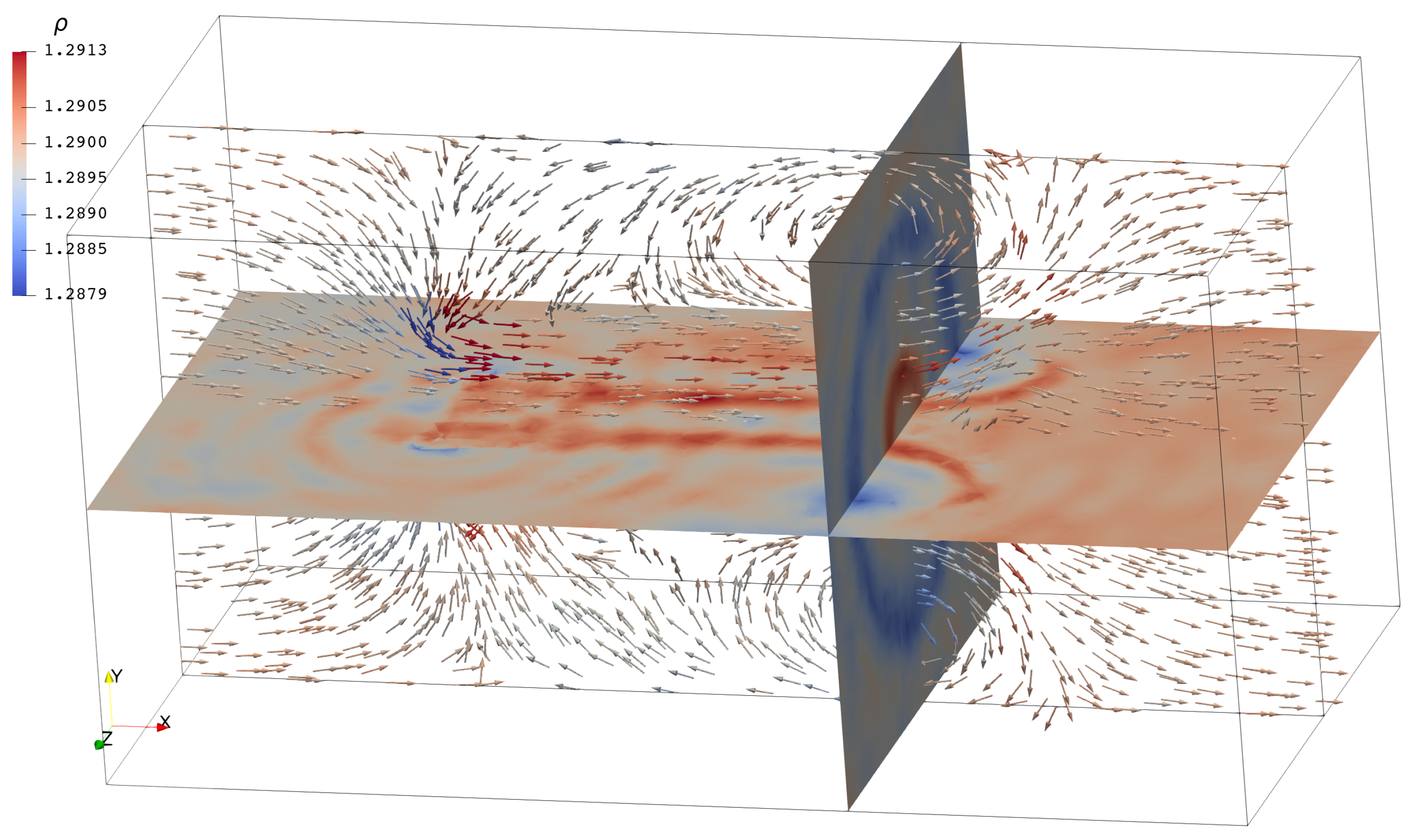
3.3. Problems with Momentum Sources

In this section, we solve two problems of rotorcraft aerodynamics using the momentum source model described in Section 2.4. The problems are set to simulate wind tunnel tests of a rotor (a pair of rotary wings), using the mesh shown in Figure 31. All of the boundaries of the outside box are solid walls, except he left and right ends, which are set as the inlet and outlet, respectively. The spherical region is the circumscribed sphere of the rotor, whose rotating axis could point in any direction. The smaller box enclosing the sphere is used for refining the mesh in the surrounding and downstream regions of the rotor.

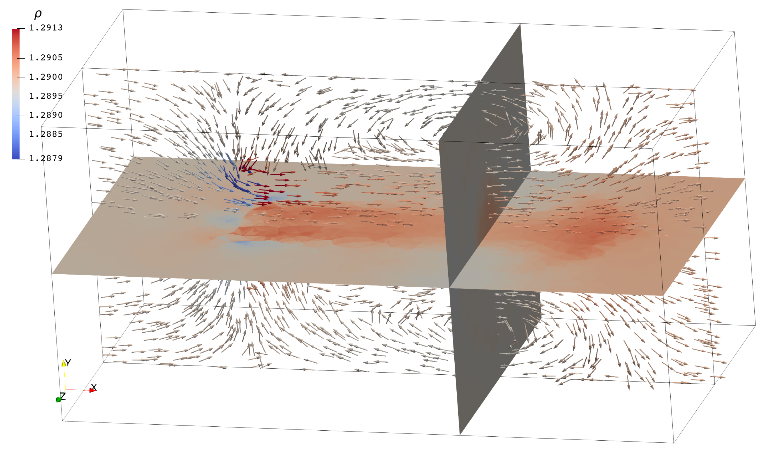
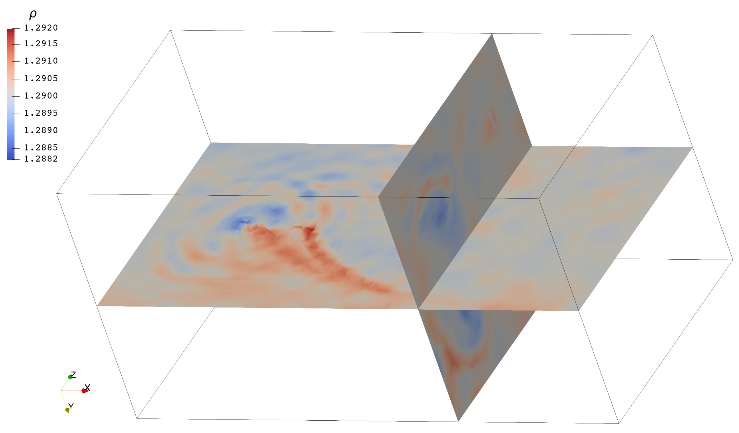
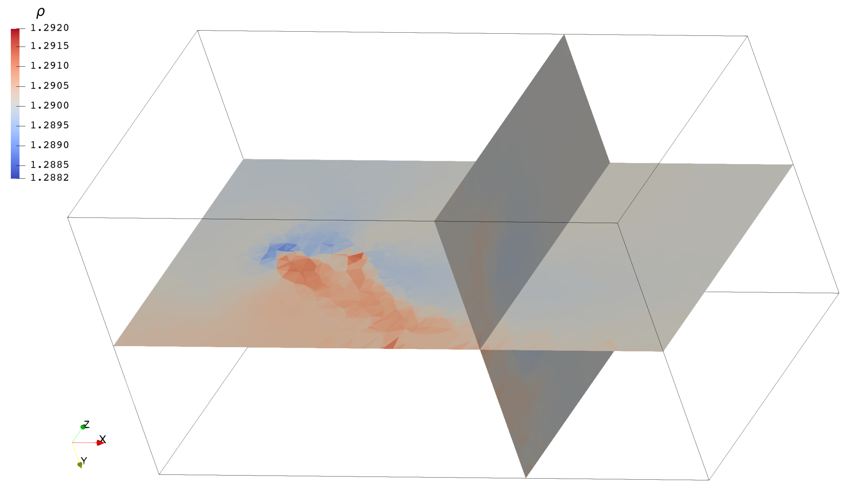
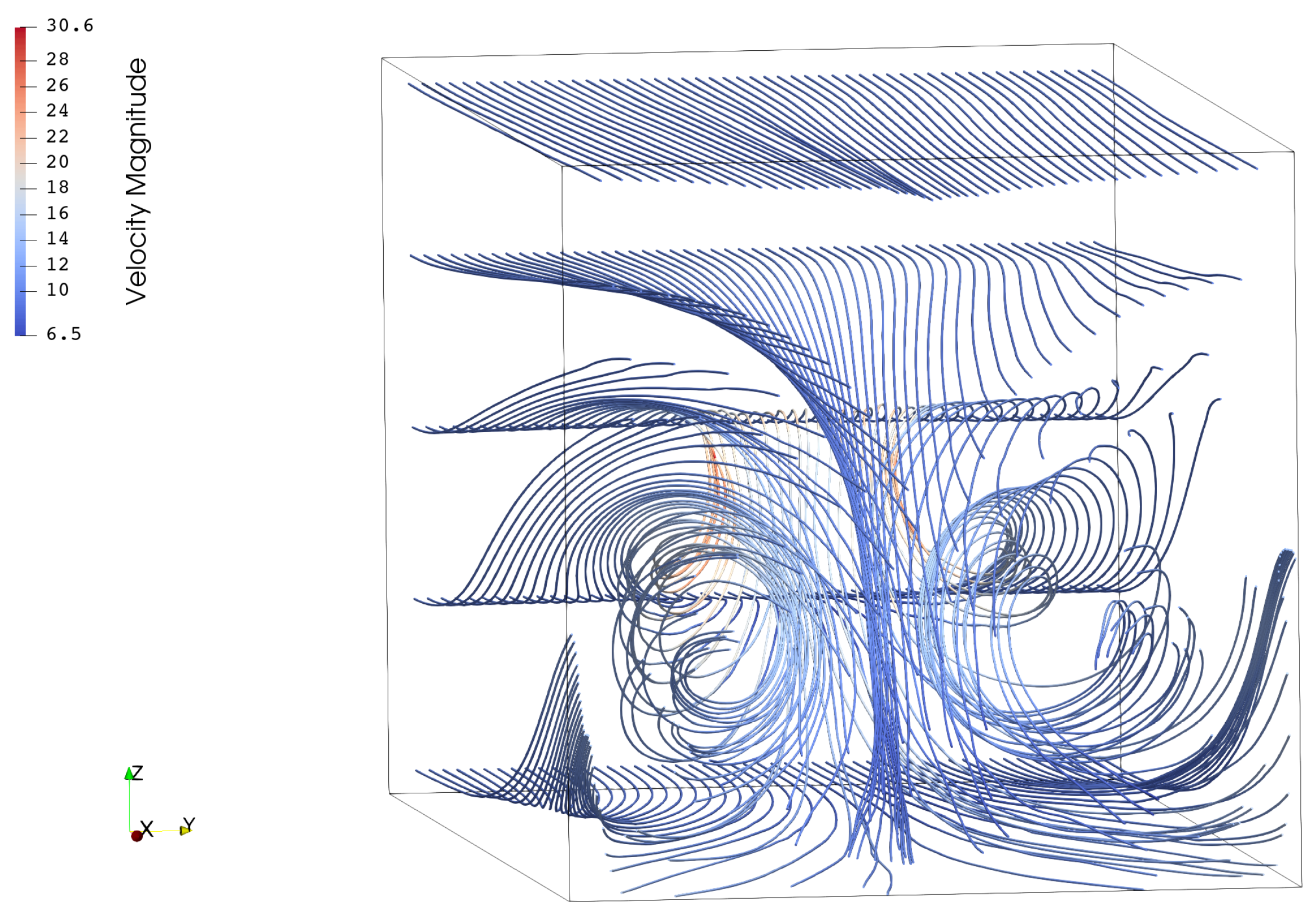
3.3.1. A Climbing Rotor

Problem 7.

Solve Equation (1) in the surroundings of a rotor, whose rotating axis points in the direction of $(-1,0,0)$. The initial condition is given as a uniform flow:

$${\left[\begin{array}{ccccc}\rho & u& v& w& p\end{array}\right]}_{t=0}=\left[\begin{array}{ccccc}1.29& 1.0& 0.0& 0.0& 101325.0\end{array}\right],$$

which is also the background state at the two ends of the wind tunnel.

Third- and first-order solutions at the same moment ($t=1$) are shown in Figure 32 and Figure 33, respectively, in which density contours and velocity directions are plotted on selected slices. Large-scale flow structures, such as the contraction of airflow near the rotor disk and the rolled-up airwake, are captured in both figures. However, finer details, such as the ripples generated from the rotor disk and the strong vortex ring in the downstream, are only visible in the third-order solution. The nearly axisymmetric flow structure is caused by the periodic movement of the rotary wings. The density of air immediately below the rotor (red) is greater than that above the rotor (blue), which means that the rotor is compressing the air flowing across it. According to Newton’s third law, the rotor must be experiencing a force in the opposite direction exerted by the air. This is where the rotor thrust comes from.

3.3.2. A Rotor in Forward Flight

Problem 8.

Solve Equation (1) in the surrounding of a rotor, whose rotating axis points in the direction of $(0,0,1)$. The initial condition is given as a uniform flow:

$${\left[\begin{array}{ccccc}\rho & u& v& w& p\end{array}\right]}_{t=0}=\left[\begin{array}{ccccc}1.29& 10.0& 0.0& 0.0& 101325.0\end{array}\right],$$

which is also the background state at the two ends of the wind tunnel.

As with the climbing problem, we plot the third- and first-order solution at the same moment ($t=1$) in Figure 34 and Figure 35, respectively. As before, both of them can capture large-scaled structures, such as the skewed and rolled-up airwakes. The rolled-up structure is more clear in Figure 36, in which streamlines are plotted and colored by the magnitude of velocity. The piecewise constant first-order solution is much vaguer and loses many details, which shows again the value of developing high-order solvers.

4. Discussion

In this article, we give a concise but complete formulation of an RKDG scheme with a compact WENO limiter for solving inviscid compressible flows, possibly with momentum sources, on three-dimensional unstructured meshes. The algorithms are implemented on top of public available libraries, which support unstructured mesh partitioning, inter-process communication and distributed memory parallelization. The correctness and accuracy of the solvers are validated by lower-dimensional reference problems. Results of real three-dimensional applications are also presented, in which complex flow structures are captured by the third-order solver even on very coarse unstructured meshes. Future works may include implementing higher-order solvers under this framework and testing them on larger meshes and on larger high-performance computing platforms.

References

1. Harten, A.; Lax, P.D.; van Leer, B. On Upstream Differencing and Godunov-Type Schemes for Hyperbolic Conservation Laws. SIAM Rev. 1983, 25, 35–61. [Google Scholar] [CrossRef]
2. Reed, W.H.; Hill, T.R. Triangular Mesh Methods for the Neutron Transport Equation; Technical Report LA-UR-73-479; Los Alamos Scientific Lab.: Los Alamos, MN, USA, 1973.
3. Chavent, G.; Salzano, G. A finite-element method for the 1-D water flooding problem with gravity. J. Comput. Phys. 1982, 45, 307–344. [Google Scholar] [CrossRef]
4. Cockburn, B.; Shu, C.W. The Runge-Kutta local projection P1-discontinuous-Galerkin finite element method for scalar conservation laws. In Proceedings of the 1st National Fluid Dynamics Conference, Cincinnati, OH, USA, 25–28 July 1988; American Institute of Aeronautics and Astronautics: Reston, VA, USA, 1988. [Google Scholar] [CrossRef] [Green Version]
5. Shu, C.W.; Osher, S. Efficient implementation of essentially non-oscillatory shock-capturing schemes. J. Comput. Phys. 1988, 77, 439–471. [Google Scholar] [CrossRef] [Green Version]
6. Shu, C.W.; Osher, S. Efficient implementation of essentially non-oscillatory shock-capturing schemes, II. J. Comput. Phys. 1989, 83, 32–78. [Google Scholar] [CrossRef]
7. Cockburn, B.; Lin, S.Y.; Shu, C.W. TVB Runge-Kutta local projection discontinuous Galerkin finite element method for conservation laws III: One-dimensional systems. J. Comput. Phys. 1989, 84, 90–113. [Google Scholar] [CrossRef] [Green Version]
8. Cockburn, B.; Hou, S.; Shu, C.W. The Runge-Kutta local projection discontinuous Galerkin finite element method for conservation laws. IV. The multidimensional case. Math. Comput. 1990, 54, 545–581. [Google Scholar] [CrossRef] [Green Version]
9. Cockburn, B.; Shu, C.W. The Runge–Kutta Discontinuous Galerkin Method for Conservation Laws V: Multidimensional Systems. J. Comput. Phys. 1998, 141, 199–224. [Google Scholar] [CrossRef]
10. Gottlieb, D.; Shu, C.W. On the Gibbs Phenomenon and Its Resolution. SIAM Rev. 1997, 39, 644–668. [Google Scholar] [CrossRef] [Green Version]
11. Sweby, P.K. High Resolution Schemes Using Flux Limiters for Hyperbolic Conservation Laws. SIAM J. Numer. Anal. 1984, 21, 995–1011. [Google Scholar] [CrossRef]
12. Harten, A.; Engquist, B.; Osher, S.; Chakravarthy, S.R. Uniformly High Order Accurate Essentially Non-oscillatory Schemes, III. J. Comput. Phys. 1997, 131, 3–47. [Google Scholar] [CrossRef]
13. Jiang, G.S.; Shu, C.W. Efficient Implementation of Weighted ENO Schemes. J. Comput. Phys. 1996, 126, 202–228. [Google Scholar] [CrossRef] [Green Version]
14. Hu, C.; Shu, C.W. Weighted Essentially Non-oscillatory Schemes on Triangular Meshes. J. Comput. Phys. 1999, 150, 97–127. [Google Scholar] [CrossRef] [Green Version]
15. Qiu, J.; Shu, C.W. Runge–Kutta Discontinuous Galerkin Method Using WENO Limiters. SIAM J. Sci. Comput. 2005, 26, 907–929. [Google Scholar] [CrossRef]
16. Zhu, J.; Qiu, J.; Shu, C.W.; Dumbser, M. Runge–Kutta discontinuous Galerkin method using WENO limiters II: Unstructured meshes. J. Comput. Phys. 2008, 227, 4330–4353. [Google Scholar] [CrossRef]
17. Zhong, X.; Shu, C.W. A simple weighted essentially nonoscillatory limiter for Runge–Kutta discontinuous Galerkin methods. J. Comput. Phys. 2013, 232, 397–415. [Google Scholar] [CrossRef]
18. Zhu, J.; Zhong, X.; Shu, C.W.; Qiu, J. Runge–Kutta discontinuous Galerkin method using a new type of WENO limiters on unstructured meshes. J. Comput. Phys. 2013, 248, 200–220. [Google Scholar] [CrossRef]
19. Pei, W.; Jiang, Y.; Li, S. An Efficient Parallel Implementation of the Runge–Kutta Discontinuous Galerkin Method with Weighted Essentially Non-Oscillatory Limiters on Three-Dimensional Unstructured Meshes. Appl. Sci. 2022, 12, 4228. [Google Scholar] [CrossRef]
20. Rajagopalan, R.G.; Mathur, S.R. Three dimensional analysis of a rotor in forward flight. In Proceedings of the 20th Fluid Dynamics, Plasma Dynamics and Lasers Conference, Buffalo, NY, USA, 12–14 July 1989; American Institute of Aeronautics and Astronautics: Reston, VA, USA, 1989. [Google Scholar] [CrossRef]
21. Rajagopalan, R.G.; Mathur, S.R. Three Dimensional Analysis of a Rotor in Forward Flight. J. Am. Helicopter Soc. 1993, 38, 14–25. [Google Scholar] [CrossRef] [Green Version]
22. Kang, N.; Sun, M. Technical Note: Prediction of the Flow Field of a Rotor in Ground Effect. J. Am. Helicopter Soc. 1997, 42, 195–198. [Google Scholar] [CrossRef]
23. Kang, N.; Sun, M. Simulated Flowfields in Near-Ground Operation of Single- and Twin-Rotor Configurations. J. Aircr. 2000, 37, 214–220. [Google Scholar] [CrossRef]
24. Shi, Y.; Xu, Y.; Zong, K.; Xu, G. An investigation of coupling ship/rotor flowfield using steady and unsteady rotor methods. Eng. Appl. Comput. Fluid Mech. 2017, 11, 417–434. [Google Scholar] [CrossRef] [Green Version]
25. Shen, W.Z.; Zhang, J.H.; Sørensen, J.N. The Actuator Surface Model: A New Navier–Stokes Based Model for Rotor Computations. J. Sol. Energy Eng. 2009, 131, 011002. [Google Scholar] [CrossRef]
26. Kim, T.; Oh, S.; Yee, K. Improved actuator surface method for wind turbine application. Renew. Energy 2015, 76, 16–26. [Google Scholar] [CrossRef]
27. Toro, E.F. Riemann Solvers and Numerical Methods for Fluid Dynamics; Springer: Berlin/Heidelberg, Germany, 2009. [Google Scholar] [CrossRef]
28. Zhang, L.; Cui, T.; Liu, H. A Set of Symmetric Quadrature Rules on Triangles and Tetrahedra. J. Comput. Math. 2009, 27, 89–96. [Google Scholar]
29. Gottlieb, S.; Shu, C.W. Total variation diminishing Runge-Kutta schemes. Math. Comput. 1998, 67, 73–85. [Google Scholar] [CrossRef] [Green Version]
30. Gottlieb, S.; Shu, C.W.; Tadmor, E. Strong Stability-Preserving High-Order Time Discretization Methods. SIAM Rev. 2001, 43, 89–112. [Google Scholar] [CrossRef]
31. Woodward, P.; Colella, P. The numerical simulation of two-dimensional fluid flow with strong shocks. J. Comput. Phys. 1984, 54, 115–173. [Google Scholar] [CrossRef]
32. Karypis, G.; Kumar, V. A Fast and High Quality Multilevel Scheme for Partitioning Irregular Graphs. SIAM J. Sci. Comput. 1998, 20, 359–392. [Google Scholar] [CrossRef]
Figure 1. Third-order solution of ρ ( t = 1.0 ) in Problem 1.
Aerospace 09 00372 g001
Figure 2. Comparison between solutions of ρ ( t = 1.0 ) in Problem 1.
Aerospace 09 00372 g002
Figure 3. Comparison between solutions given by various hp pairs.
Aerospace 09 00372 g003
Figure 4. Third-order solution of ρ ( t = 0.5 ) in Problem 2.
Aerospace 09 00372 g004
Figure 5. Comparison between solutions of ρ ( t = 0.5 ) in Problem 2.
Aerospace 09 00372 g005
Figure 6. Third-order solution of ρ ( t = 0.4 ) in Problem 3.
Aerospace 09 00372 g006
Figure 7. Comparison between solutions of ρ ( t = 0.4 ) in Problem 3.
Aerospace 09 00372 g007
Figure 8. A coarse ( h = 1 / 20 ) mesh for solving Problem 4. This mesh is too coarse to capture details of the flow field but clear enough to demonstrate the distribution of nodes and cells. Actually, we use a much finer ( h = 1 / 200 ) mesh to produce Figure 9, Figure 10, Figure 11, Figure 12, Figure 13, Figure 14, Figure 15, Figure 16, Figure 17, Figure 18 and Figure 19.
Aerospace 09 00372 g008
Figure 9. Third-order solution of Problem 4 at t = 0.2 on an h = 1 / 200 mesh.
Aerospace 09 00372 g009
Figure 10. Third-order solution of Problem 4 at t = 0.4 on an h = 1 / 200 mesh.
Aerospace 09 00372 g010
Figure 11. Third-order solution of Problem 4 at t = 0.6 on an h = 1 / 200 mesh.
Aerospace 09 00372 g011
Figure 12. Third-order solution of Problem 4 at t = 0.8 on an h = 1 / 200 mesh.
Aerospace 09 00372 g012
Figure 13. Third-order solution of Problem 4 at t = 1.0 on an h = 1 / 200 mesh.
Aerospace 09 00372 g013
Figure 14. Third-order solution of Problem 4 at t = 1.2 on an h = 1 / 200 mesh.
Aerospace 09 00372 g014
Figure 15. Third-order solution of Problem 4 at t = 2.0 on an h = 1 / 200 mesh.
Aerospace 09 00372 g015
Figure 16. Third-order solution of Problem 4 at t = 2.4 on an h = 1 / 200 mesh.
Aerospace 09 00372 g016
Figure 17. Third-order solution of Problem 4 at t = 2.8 on an h = 1 / 200 mesh.
Aerospace 09 00372 g017
Figure 18. Third-order solution of Problem 4 at t = 3.2 on an h = 1 / 200 mesh.
Aerospace 09 00372 g018
Figure 19. Third-order solution of Problem 4 at t = 4.0 on an h = 1 / 200 mesh.
Aerospace 09 00372 g019
Figure 20. A zoomed-in view of the most important boundaries of the mesh for solving problems in Section 3.2.
Aerospace 09 00372 g020
Figure 21. Streamlines given by the first-order solution of Problem 5.
Aerospace 09 00372 g021
Figure 22. Streamlines given by the third-order solution of Problem 5.
Aerospace 09 00372 g022
Figure 23. Comparison between the third-order solution (left half) and the first-order solution (right half) of Problem 5.
Aerospace 09 00372 g023
Figure 24. Density contour obtained from the first-order solution of Problem 6.
Aerospace 09 00372 g024
Figure 25. Density contour obtained from the third-order solution of Problem 6.
Aerospace 09 00372 g025
Figure 26. Comparison between the third-order solution (upper half) and the first-order solution (lower half) of Problem 6 on the z = 0 surface (top view).
Aerospace 09 00372 g026
Figure 27. Comparison between the third-order solution (upper half) and the first-order solution (lower half) of Problem 6 on the z = 0 surface (bottom view).
Aerospace 09 00372 g027
Figure 28. A 100-part partitioning of the mesh used for solving problems in Section 3.2.
Aerospace 09 00372 g028
Figure 29. Distribution of cells in the mesh partitioning given in Figure 28.
Aerospace 09 00372 g029
Figure 30. Parallel efficiency of the third-order solver for solving Problem 6.
Aerospace 09 00372 g030
Figure 31. A schematic mesh for solving problems in Section 3.3.
Aerospace 09 00372 g031
Figure 32. Third-order solution of Problem 7 at t = 1 .
Aerospace 09 00372 g032
Figure 33. First-order solution of Problem 7 at t = 1 .
Aerospace 09 00372 g033
Figure 34. Third-order solution of Problem 8 at t = 1 .
Aerospace 09 00372 g034
Figure 35. First-order solution of Problem 8 at t = 1 .
Aerospace 09 00372 g035
Figure 36. Streamlines of the solution in Figure 34.
Aerospace 09 00372 g036