Layout Design of Strapdown Array Seeker and Extraction Method of Guidance Information

Abstract

This paper proposed a multi-view surface array to enlarge the field-of-view (FOV) from 45° × 45° to 72° × 75° and improve the estimation precision of guidance information. First, based on circular and rectangular FOV sensors, the superposition characteristics of FOV in the +-shaped layout and the X-shaped layout were explored and analyzed. Secondly, normalization processing was applied to obtain the equivalent measurement value of the central sensor and the corresponding error distribution. Based on such measurement value and error distribution, the filtering model could be constructed, which could effectively solve the problem of observation number variation caused by multiple sensors. Thirdly, a multivariate iterated extended Kalman filter (MIEKF) was proposed to make full use of multiple measurements. By iterating multiple unequal observations and making full use of the known error distribution information, the noise of filtered data was found to be effectively reduced and the estimation precision of guidance information was improved. Finally, based on a 6-DOF trajectory simulation, the correctness and effectiveness of the proposed method were verified. Simulation results show that MIEKF can improve the estimation accuracy of the line-of-sight (LOS) angle by at least 30% and the estimation accuracy of the LOS angle rate by nearly 80% compared with EKF.

1. Introduction

Seekers are usually installed on the head of the missile, and they usually use infrared, laser, radar, and other sensors. The seekers can detect the target and transmit its information to the computer on the missile. With target information, the missile can hit the target through guidance and control. As the eyes of missiles, seekers should be able to see “accurately” and “widely” in a complex environment [1]. In the past, due to the FOV constraint of seekers, the maneuverability of missiles was limited. Thus, a number of guidance laws with FOV constraint were developed. An optimal guidance law was designed to control the impact angle and the impact point under the FOV constraint in [2]. Based on the two-stage proportional navigation guidance law, several scholars proposed that, by designing the proportional navigation guidance (PNG) coefficients in different stages, the impact angle and impact point constraints can be realized under the FOV constraint [3,4,5]. A two-stage biased PNG method, which can accurately strike fixed and moving targets under the FOV constraint was proposed in [6]. A guidance law, based on the sliding mode control method, which considered the FOV limitations as well as the impact angle and time constraints, was proposed in [7]. A new PNG method was studied to achieve omnidirectional attacks on moving targets under the FOV and impact angle constraints in [8]. A guidance law for the FOV constraints by means of the backstepping control method was studied in [9]. The capture region of the composite guidance law under the FOV constraint of the strapdown seeker was analyzed in [10]. A three-dimensional impact time control guidance considering field-of-view constraints and time-varying velocity was proposed in [11]. All of the aforementioned methods were based on the assumption that the angle of attack is zero, and the FOV angle constraint is converted into the angle of view constraint. However, as indicated in previous research [12], missiles often require a large angle of attack to provide a large normal overload during maneuvering. Therefore, in the actual application process, even if some methods of controlling the FOV angle are adopted, there is still the possibility of target loss. In order to solve this problem, the FOV should be enlarged so as to reduce the limitations of aircraft maneuverability caused by FOV constraints.

The guidance accuracy largely depends on the accuracy of the seeker. Seekers can be divided into platform seeker and strapdown seeker. The platform seeker contains a sensor and a stabilization platform. The stable platform can keep the seeker aiming at the target. Unlike the platform seeker, the sensor of the strapdown seeker is fixed on the head of the missile. So, the aiming direction of its sensor will change with the movement of the missile. The platform seeker was adopted in the earliest precision-guided missile. The inertial platform established by the high-precision frame can isolate the interference of the seeker caused by the movement of the missile. Through the mechanical gimbal, platform, seekers can easily track the target and enlarge the FOV angle. However, due to the existence of the gimbal, the guidance information is subject to the constraints of maximum overload, maximum tracking rate, and others. Moreover, there are difficulties in miniaturizing and reducing the costs [13,14]. Strapdown seekers effectively avoid such problems, but they also face other challenges. The FOV constraint and low accuracy are the main problems. For platform seekers, the frame structure ensures that the FOV easily reaches 90°, while that of strapdown seekers usually only reaches 30°~45°. The development of strapdown seekers with large FOV has become a trending research topic in recent years [15]. For infrared imaging seekers, when the pixels are fixed, a “wide” view and an “accurate” view are a pair of contradictory constraints. A larger FOV will introduce more background radiation noise, which would shorten the detection range and reduce immunity [16]. In order to enlarge the FOV, the U.S. military proposed simulating the compound eyes of insects to develop a bionic seeker with a large FOV, which can detect with omni-directionality. The aim of this research was to obtain the trajectory of the target, while preventing the target from being lost [17,18]. The bionic compound eye seeker is a typical array seeker, which consists of many small eyes with the same structure and function. A spherical compound eye that consists of an array of micro-lenses was developed in [19,20]. The TOMBO artificial compound eye structure, which is a planar array, was proposed in [21,22]. Based on the image fusion algorithm, array images are fused to obtain reconstructed images. An artificial compound eye made up of 7734 eye units with a diameter of 100 microns was designed in [23]. Experimental results show that its FOV angle can reach 120°. A compound eye with a 180° FOV angle based on 10.5 mm × 10.5 mm CCD cameras was designed in [24]. The above bionic compound eyes are based on a visible lens array, and the large field of view seekers are obtained through image reorganization. However, the computation of image processing will increase sharply with the increase of sensors. Thus, further research is needed to realize real-time processing in missiles. Furthermore, visible light is easily interfered with by the environment, and it is weak in detecting long-range targets. A distributed strapdown seeker, which installed four fiber detectors on the cruciform wings to receive reflected laser light, was designed in [25]. It belongs to a planar array, which faces difficulties in expanding the FOV. Inspired by compound eyes, an infrared array seeker is designed in this paper. Five infrared sensors are installed on the missile head. It belongs to curved array which can effectively enlarge the FOV.

A large number of estimation methods for strapdown seeker guidance information have been proposed after decades of development. The LOS angle rate of strapdown seeker is estimated by the filter in previous studies [26,27,28]. The unscented Kalman filter (UKF) was applied to guidance information extraction in [29]. Based on UKF, an adaptive UKF, which could improve the accuracy of the system by predicting the residual error, was proposed in [30]. Based on the extended Kalman filter (EKF), an adaptive and predictive filter was proposed to estimate strapdown seeker guidance in [31]. Additionally, a particle filter [32], nonlinear filter [33,34,35], and other filters have been successfully applied to the estimation of strapdown seeker guidance information. The aforementioned methods are based on a single sensor in which the optical axis coincides with the principal axis of the missile. The object of this paper was the multi-sensor surface array seeker. Therefore, the aforementioned methods could be used as references but were not completely applicable. Regarding the aforementioned problems, the main contributions of the present study are as follows:

(1)

The layout of the multi-sensor was explored;

(2)

An MIEKF was constructed to estimate guidance information;

(3)

Based on the 6-DOF trajectory simulation model, the performance of the monocular seeker and the multi-eye seeker were compared and analyzed, and the performance of the EKF, Iterated EKF (IEKF), and MIEKF were also compared.

The remainder of this article is arranged as follows: the layout of multi-purpose sensors is discussed in Section 2; the LOS rate estimation method and the guidance information extraction model are introduced in Section 3; the constructed filter estimation model is presented in Section 4; a large number of simulation results are provided in Section 5; and the conclusion is given in Section 6.

2. Layout Design of the Sensors

Five independent sensors were explored in the present study. In order to facilitate this research, the following assumptions were made:

• The head of the missile is ellipsoidal, and the sensor mounting plane is tangent to the shell;
• Each sensor is qualified, and thus, the measurement error distribution is known;
• Each sensor has its own independent signal processor and can output LOS angle information;
• Through installation and adjustment, the focuses of each sensor are at the same point as the body axes of the missile.

According to Assumption 1, the sight of each senser would not be blocked by the missile, and the FOV is therefore only related to the individual parameters of each sensor. Assumption 2 defines the composition of the measurement variance matrix. Assumption 3 demonstrates that the focus of the present study was on the layouts of the array sensors, as well as the guidance information extraction method, rather than the sensor signal processing and target identification method. Notably, no matter how the installations were adjusted, the focal points of the sensors could not be exactly the same. However, the error distance between the focal points was a minimum relative to the LOS range, and the influence on the estimation of guidance information was negligible. As such, Assumption 4 was established. There are two kinds of FOV shapes of the seeker: circular and rectangular. Based on the fundamental principle that the FOV angle of each sensor was 45°, the +-shaped layout and the X-shaped layout were examined.

The sensors are mounted on the nose cone of the missile, as shown in Figure 1a,b, which demonstrate how sensors are installed in a +-shaped layout.

Figure 1c,d show how sensors are installed in an X-shaped layout. The +-shaped and X-shaped layouts depend on the position of the sensors relative to the missile’s principal symmetry plane. As shown in (a), the principal symmetric plane can be described as $x_{1}o{y}_1$ in the BCS B. It determines the installation of the inertial measurement unit and actuators. For non-rotating missiles, the principal symmetric plane usually remains stable and perpendicular to the horizontal plane during flight. Figure 2 is the back vision project.

It can be seen from Figure 2a that in the +-shaped layout, sensors 2 and 4 are on the principal symmetric plane, and the line of sensors 3 and 5 is perpendicular to the principal symmetric plane. It can be seen from Figure 2b that in the X-shaped layout, the angle between the principal symmetric plane and the line of sensors 2 and 4 is 45°, and the angle between the principal symmetric plane and the line of sensors 3 and 5 is 45° too.

The relevant coordinate systems and the conversion relations were involved in the following derivation, using a previous study as a reference [36]. Notably, the order of 2-3-1 was adopted for the coordinate transformation in the present study. The transformation relationship is summarized in Figure 3.

The sensor coordinate system (SCS) I can be defined as: the sensor focus being selected as the origin of the coordinate system, the x-axis being perpendicular to the focal plane from the origin, the y-axis being parallel to the focal plane and pointing upwards, and the z-axis being determined by the right-handed coordinate system criterion. The SCS I is shown in Figure 4.

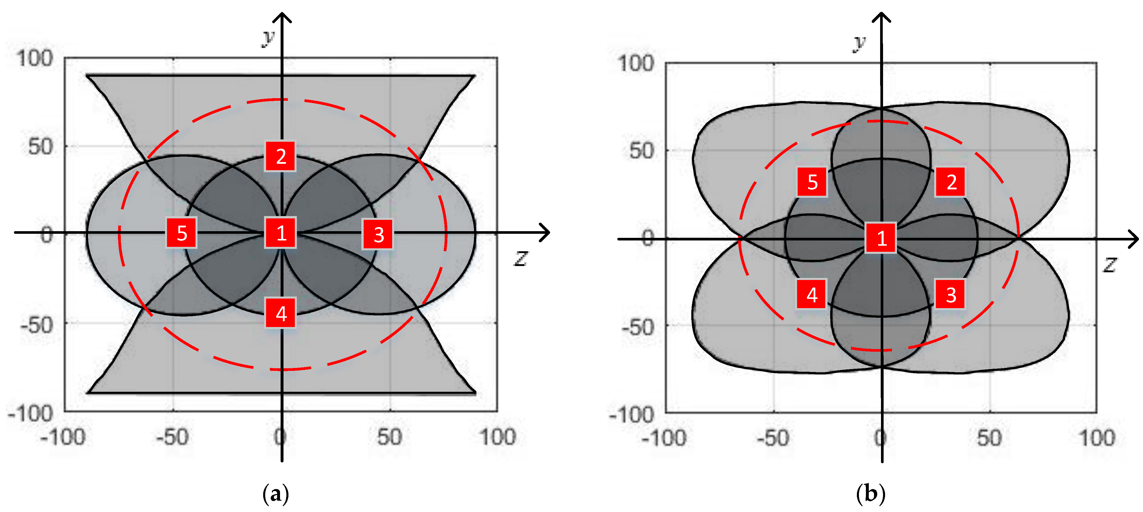
2.1. Circular FOV Sensors

Observed from the tail of the missile, the sensor was projected onto a two-dimensional plane as follows.

According to the relationship between the SCS I, body fixed coordinate system (BCS) $B$ and the installation angle, the transformation matrix from the BCS $B$ to the SCS I could be recorded as:

$$I_{Bi}=\left[\begin{array}{ccc}\cos ({\lambda }_{ei})& \sin ({\lambda }_{ei})& 0\\ -\sin ({\lambda }_{ei})& \cos ({\lambda }_{ei})& 0\\ 0& 0& 1\end{array}\right]\left[\begin{array}{ccc}\cos ({\lambda }_{ai})& 0& -\sin ({\lambda }_{ai})\\ 0& 1& 0\\ \sin ({\lambda }_{ai})& 0& \cos ({\lambda }_{ai})\end{array}\right]$$

(1)

where subscript i indicates the sensor number. Combined with Figure 1 and Figure 4, the angle in the equation could be obtained, and the results are shown in

Table 1. Transformation angles from BCS B to SCS I.

Sensor No.	+-Shaped Layout		X-Shaped Layout
	${\mathit{\lambda }}_{\mathit{e}}\left[\text{°}\right]$	${\mathit{\lambda }}_{\mathit{a}}\left[\text{°}\right]$	${\mathit{\lambda }}_{\mathit{e}}\left[\text{°}\right]$	${\mathit{\lambda }}_{\mathit{a}}\left[\text{°}\right]$
1	0	0	0	0
2	45	0	45/$\sqrt{2}$	−45/$\sqrt{2}$
3	0	−45	−45/$\sqrt{2}$	−45/$\sqrt{2}$
4	−45	0	45/$\sqrt{2}$	−45/$\sqrt{2}$
5	0	45	45/$\sqrt{2}$	45/$\sqrt{2}$

.

Sensor No.1 was located in the center of the head of the missile, and the coordinate system was the same as the BCS B. General monocular sensors are installed in the same way. Assuming the LOS range is r, when the target is in the view of sensor i, the sensor will output the target LOS azimuth angle $q_{ai}$ and the LOS altitude angle $q_{ei}$. Therefore, in the SCS I, the target can be expressed as:

$$\left[\begin{array}{c}{x}_{Ii}\\ y_{Ii}\\ z_{Ii}\end{array}\right]=\left[\begin{array}{c}r\cos (q_{ei})\cos (q_{ai})\\ r\sin (q_{ei})\\ -r\sin (q_{ai})\cos (q_{ei})\end{array}\right]$$

(2)

being transformed into the BCS B as:

$$\begin{array}{cc}\left[\begin{array}{c}{x}_b\\ y_b\\ z_b\end{array}\right]\hfill & =I_{Bi}{}^{\prime }\left[\begin{array}{c}{x}_{Ii}\\ y_{Ii}\\ z_{Ii}\end{array}\right]\hfill \\ \hfill & =\left[\begin{array}{ccc}{r}_{11}& r_{12}& r_{13}\\ r_{21}& r_{22}& r_{23}\\ r_{31}& r_{32}& r_{33}\end{array}\right]\left[\begin{array}{c}{x}_{Ii}\\ y_{Ii}\\ z_{Ii}\end{array}\right]\hfill \end{array}$$

(3)

According to the definition of the body LOS coordinate system (BLCS) L, the target is expressed as ${\left[\begin{array}{ccc}r& 0& 0\end{array}\right]}^T$ in the BLCS L, which transforms the target into the BCS B as:

$$\left[\begin{array}{c}{x}_b\\ y_b\\ z_b\end{array}\right]=B_L\left[\begin{array}{c}r\\ 0\\ 0\end{array}\right]=\left[\begin{array}{c}r\cos (q_a)\cos (q_e)\\ r\sin (q_e)\\ -r\sin (q_a)\cos (q_e)\end{array}\right]$$

(4)

On the basis of Equations (3) and (4), the relationship between the body LOS angle and the LOS angle can be established as:

$$\left[\begin{array}{c}\cos (q_a^i)\cos (q_e^i)\\ \sin (q_e^i)\\ -\sin (q_a^i)\cos (q_e^i)\end{array}\right]=\left[\begin{array}{c}A\\ B\\ C\end{array}\right]$$

(5)

$$q_e^i=\arcsin (B)$$

(6)

$$q_a^i=\arctan (-C/A)$$

(7)

where

$$\{\begin{array}{l}A=r_{11}\cos \left(q_{ai}\right)\cos (q_{ei})+r_{12}\sin (q_{ei})-r_{13}\cos (q_{ei})\sin (q_{ai})\\ B=r_{21}\cos (q_{ai})\cos (q_{ei})+r_{22}\sin (q_{ei})\\ C=r_{31}\cos (q_{ai})\cos (q_{ei})+r_{32}\sin (q_{ei})-r_{33}\cos (q_{ei})\sin (q_{ai})\end{array}$$

(8)

The circular FOV sensor’s FOV boundary can be expressed as:

$$\{\begin{array}{l}{q}_{edg}^e=\frac{\pi }{4}\sin (\xi )\\ q_{edg}^a=\frac{\pi }{4}\cos (\xi )\end{array}\begin{array}{cc}& \xi \in (0,\pi )\end{array}$$

(9)

The results of combining Equations (6) and (7), and the subsequent transformation into body fixed FOV, are shown in Figure 5.

The coordinate system established in Figure 5 can be defined as follows: the y-axis represents the body LOS altitude angle; the z-axis represents the inverse number of body LOS azimuth angles; the red square represents the sensors; the numbers represent the sensors’ No.; and the shadow represents the area covered by the sensor’s FOV, the shade of the shadow being determined by the number of sensors, with the darker the shadow indicating that more sensors are detected. As shown in Figure 5, the array sensor could effectively expand the seeker’s FOV. Owing to the FOV’s irregular superposition, there would inevitably be uncovered areas, referred to as blind areas. Thus, a characterization index is indicated for the non-blind areas covered by the biggest circle: non-blind area FOV $\varphi$, which is represented by the red dotted line area. In the +-shaped layout, the radius of the non-blind area FOV ${\varphi }_r$ was 75.1°, while in the X-shaped layout, the radius of the non-blind area FOV ${\varphi }_r$ was 63.8°. Comparing the +-shaped layout and the X-shaped layout, the +-shaped layout has bigger non-blind areas. However, there was a lower number of sensors around the y-axis, and a higher number of sensors in the diagonal area. The X-shaped layout had a relatively small FOV in non-blind areas, but there were more sensors around the y-axis. During the guidance information estimation process, if the amount of observation was higher, the precision of the estimated parameters was higher. Therefore, in the layout design, the targets should be placed in the darker areas. The targets should be placed as described due to the measurement data precision near the principal symmetric plane. In order to hit the target, the missile usually flies towards the target, and the lateral azimuth angle is small when the rolling and yawing channels are stable. Ideally, if the target stays in the incidence plane, the target will only move on the y-axis in the aforementioned coordinate system. The precision of all nearby measurement data is particularly important.

According to the aforementioned analysis, the +-shaped layout has advantages in terms of fully expanding the FOV, while the X-shaped layout has advantages in terms of the higher number of sensors around the y-axis, which effectively improves the data precision and facilitates a clearer view of targets for missiles. If the sensor has high precision and satisfies the needs of independent use, and the purpose of the array is to enlarge the FOV angle, then the +-shaped layout is the optimal choice. If the sensor has low precision, and the aim is to improve data precision while enlarging the FOV angle, then the X-shaped layout is the optimal choice.

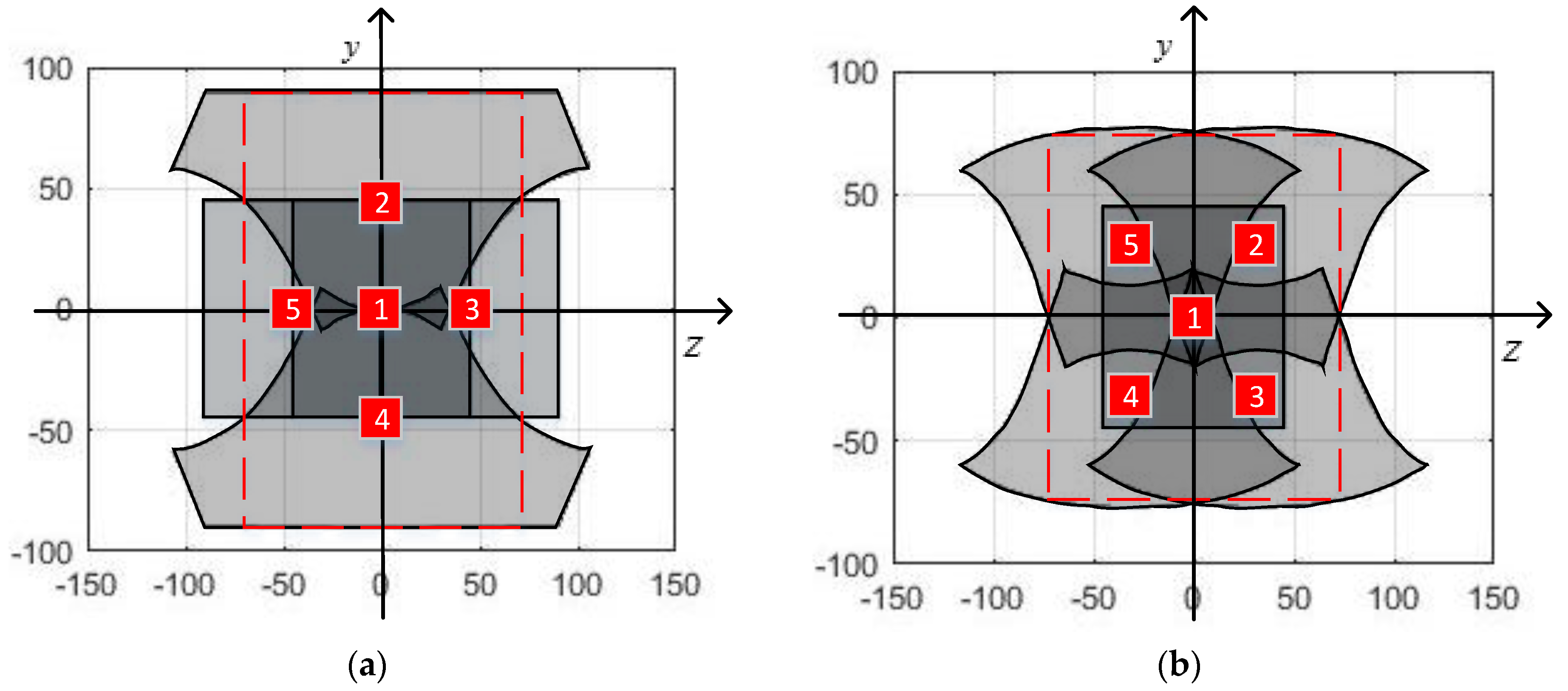
2.2. Rectangular FOV Sensor

Following the aforementioned analysis, the field coverage images behind the rectangular FOV sensor array can be easily represented, as shown in Figure 6. The FOV angle of the +-shaped layout was 70.5° × 90°, while that of the X-shaped layout was 72° × 75°. An observation can be made that through the +-shaped layout, the maximum FOV areas were enlarged, and the central sensor FOV was strengthened, which could be observed by at least four sensors at the same time. However, the area out of the central sensor FOV could only be covered by one sensor. Even the FOV of the X-shaped layout was smaller, but around the y-axis, coverage could be provided by at least two sensors. Furthermore, in the central area, coverage could be up to five sensors, which is an ideal sensor layout. Based on the notable properties of the X-shaped layout, the layout method of guidance information extraction was the X-shaped layout.

3. Strapdown Array Seeker Guidance Information Extraction Model

Differing from monocular seekers, strapdown array seekers allow for multiple observations that are not in the same coordinate system. In the working process of seekers, the optical axes of sensors are not coincident due to the surface array, and their FOV are different, which causes the number of visible sensors to change. In this situation, if all the sensor outputs are taken as observations to filter and estimate the guidance information, it will be very difficult to establish the state equation and observation equation. Thus, in the present study, normalization processing was performed with different senor measurement results, and the measurement results and errors were unified into the equivalent measurement results of the center sensor. Furthermore, the filter equation could be established, and guidance information could be extracted.

3.1. Normalization Processing

The relationship between the fixed body LOS angle and the sensor LOS angle has been established. Considering the measurement noise, the following equations could be obtained by means of Equations (6)–(8):

$$\begin{array}{cc}{q}_e^i\hfill & =g_1(q_{ai},q_{ei})+v_{1i}\hfill \\ \hfill & =\arcsin (B)+v_{1i}\hfill \end{array}$$

(10)

$$\begin{array}{cc}{q}_a^i\hfill & =g_2(q_{ai},q_{ei})+v_{2i}\hfill \\ \hfill & =\arctan (-C/A)+v_{2i}\hfill \end{array}$$

(11)

where $v_{1i}$ and $v_{2i}$ represent the measurement noises of $q_e^i$ and $q_a^i$ in the BCS B. Assuming the original measurement data $q_{ei}$ and $q_{ai}$ have measurement noises $w_{1i}$ and $w_{2i}$, according to the error transfer theory, the $v_{1i}$ and $v_{2i}$ can be denoted as:

$$v_{1i}=\frac{\partial g_1}{\partial q_{ei}}{w}_{1i}+\frac{\partial g_1}{\partial q_{ai}}{w}_{2i}$$

(12)

$$v_{2i}=\frac{\partial g_2}{\partial q_{ei}}{w}_{1i}+\frac{\partial g_2}{\partial q_{ai}}{w}_{2i}$$

(13)

Combined with Equations (8), (10), and (11):

$$\{\begin{array}{cc}\frac{\partial g_1}{\partial q_{ei}}\hfill & =\frac{-r_{21}\cos \left(q_{ai}\right)\sin (q_{ei})+r_{22}\cos (q_{ei})}{\sqrt{1-B^2}}\hfill \\ \frac{\partial g_1}{\partial q_{ai}}\hfill & =\frac{-r_{21}\sin \left(q_{ai}\right)\cos (q_{ei})}{\sqrt{1-B^2}}\hfill \\ \frac{\partial g_2}{\partial q_{ei}}\hfill & =\frac{C\left(-r_{11}\cos \left(q_{ai}\right)\sin (q_{ei})+r_{12}\cos (q_{ei})+r_{13}\sin (q_{ei})\sin (q_{ai})\right)}{A^2+C^2}\hfill \\ \hfill & -\frac{A\left(-r_{31}\cos \left(q_{ai}\right)\sin (q_{ei})+r_{32}\cos (q_{ei})+r_{33}\sin (q_{ei})\sin (q_{ai})\right)}{A^2+C^2}\hfill \\ \frac{\partial g_2}{\partial q_{ai}}\hfill & =\frac{C\left(-r_{11}\sin \left(q_{ai}\right)\cos (q_{ei})-r_{13}\cos (q_{ei})\cos (q_{ai})\right)}{A^2+C^2}\hfill \\ \hfill & -\frac{A\left(-r_{31}\sin \left(q_{ai}\right)\cos (q_{ei})-r_{33}\cos (q_{ei})\cos (q_{ai})\right)}{A^2+C^2}\hfill \end{array}$$

(14)

Taking the variances for noises $v_{1i}$ and $v_{2i}$:

$$D(v_{1i})={\left(\frac{\partial g_1}{\partial q_{ei}}{w}_{1i}\right)}^2+2\frac{\partial g_2}{\partial q_{ei}}\frac{\partial g_2}{\partial q_{ai}}\mathrm{cov}(w_{1i},w_{2i})+{\left(\frac{\partial g_1}{\partial q_{ai}}{w}_{2i}\right)}^2$$

(15)

$$D(v_{1i})={\left(\frac{\partial g_2}{\partial q_{ei}}{w}_{1i}\right)}^2+2\frac{\partial g_2}{\partial q_{ei}}\frac{\partial g_2}{\partial q_{ai}}\mathrm{cov}(w_{1i},w_{2i})+{\left(\frac{\partial g_2}{\partial q_{ai}}{w}_{2i}\right)}^2$$

(16)

Since the altitude angle errors and azimuth angle errors are independent during the measurement process, the covariance $\mathrm{cov}(w_{1i},w_{2i})$ = 0, and the noise variances can be written as:

$$D(v_{1i})={\left(\frac{\partial g_1}{\partial q_{ei}}{w}_{1i}\right)}^2+{\left(\frac{\partial g_1}{\partial q_{ai}}{w}_{2i}\right)}^2$$

(17)

$$D(v_{1i})={\left(\frac{\partial g_2}{\partial q_{ei}}{w}_{1i}\right)}^2+{\left(\frac{\partial g_2}{\partial q_{ai}}{w}_{2i}\right)}^2$$

(18)

So, the measurement results and their error noise have been unified.

3.2. System State Equation

After normalization processing, the filter equation could be established on the equivalent measurement results based on the center sensor. According to the relative motion relationship between the missile and the target, the following mathematical model could be established:

$$\{\begin{array}{l}R=R_T-R_M\\ V=V_T-V_M\\ a=a_T-a_M\end{array}$$

(19)

where ${}_T$ represents the target; ${}_M$ represents the missile; and R, V, and a represent the relative LOS range, speed, and acceleration, respectively. In the LOS coordinate system (LCS) $S$, the rotation angular velocity of the LCS $S$ relative to the inertial coordinate system is:

$${\omega }_s=\dot{\eta }\sin \epsilon i_s+\dot{\eta }\cos \epsilon j_s+\dot{\epsilon }{k}_s$$

(20)

where $i_s$, $j_s$, and $k_s$ represent the unit vector in the LCS S. In the LCS S, the relative LOS range could be defined as:

$$R_s=r{i}_s$$

(21)

$$\begin{array}{cc}{i}_s\hfill & ={\omega }_s\times i_s\hfill \\ \hfill & =\left|\begin{array}{ccc}{i}_s& j_s& k_s\\ \dot{\eta }\sin \epsilon & \dot{\eta }\cos \epsilon & \dot{\epsilon }\\ 1& 0& 0\end{array}\right|\hfill \\ \hfill & =\dot{\epsilon }{j}_s-\dot{\eta }\cos \epsilon k_s\hfill \end{array}$$

(22)

Similarly:

$${\dot{j}}_s=-\dot{\epsilon }{i}_s+\dot{\eta }\sin \epsilon k_s$$

(23)

$${\dot{k}}_s=\dot{\eta }\cos \epsilon i_s-\dot{\eta }\sin \epsilon j_s$$

(24)

The relative velocity derived from the relative position could be denoted as:

$$\begin{array}{cc}V\hfill & =R_s\hfill \\ \hfill & =\dot{r}{i}_s+r{\dot{i}}_s\hfill \\ \hfill & =\dot{r}{i}_s+r\dot{\epsilon }{j}_s-r\dot{\eta }\cos \epsilon k_s\hfill \end{array}$$

(25)

The relative acceleration derived from the relative velocity could be denoted as:

$$\begin{array}{cc}{\dot{a}}_s\hfill & =\dot{V}\hfill \\ \hfill & =(\ddot{r}-r{\dot{\epsilon }}^2-r{\dot{\eta }}^2{\cos }^2\epsilon )i_s+(2\dot{r}\dot{\epsilon }+r\ddot{\epsilon }+r{\dot{\eta }}^2\cos \epsilon \sin \epsilon )j_s\hfill \\ \hfill & +(2r\dot{\epsilon }\dot{\eta }\sin \epsilon -2\dot{r}\dot{\eta }\cos \epsilon -r\ddot{\eta }\cos \epsilon )k_s\hfill \end{array}$$

(26)

When the missile attacks fixed or low-speed targets on the ground, the assumption is that the acceleration in the y-axis direction and the z-axis direction is zero in the LOS coordinate system. Thus:

$$\{\begin{array}{l}2\dot{r}\dot{\epsilon }+r\ddot{\epsilon }+r{\dot{\eta }}^2\cos \epsilon \sin \epsilon =0\\ 2r\dot{\epsilon }\dot{\eta }\sin \epsilon -2\dot{r}\dot{\eta }\cos \epsilon -r\ddot{\eta }\cos \epsilon =0\end{array}$$

(27)

Taking $x=\left[\begin{array}{cccc}\epsilon & \dot{\epsilon }& \eta & \dot{\eta }\end{array}\right]$ as the state variable, the system state equation could be obtained by means of Equation (27) as follows:

$$\{\begin{array}{l}{\dot{x}}_1=x_2\\ {\dot{x}}_2=-2\frac{\dot{r}}{r}{x}_2-x_4{}^2\cos x_1\sin x_1\\ {\dot{x}}_3=x_4\\ {\dot{x}}_4=2x_4{x}_2\tan x_1-2\frac{\dot{r}}{r}{x}_4\end{array}$$

(28)

3.3. System Observation Equation

In the LCS S and the BLCS L, the target can be expressed as ${\left[\begin{array}{ccc}r& 0& 0\end{array}\right]}^T$. By converting the target position from the BLCS L to the BCS B:

$$\left[\begin{array}{c}{x}_b\\ y_b\\ z_b\end{array}\right]=B_L\left[\begin{array}{c}r\\ 0\\ 0\end{array}\right]=\left[\begin{array}{c}r\cos (q_a)\cos (q_e)\\ r\sin (q_e)\\ -r\sin (q_a)\cos (q_e)\end{array}\right]$$

(29)

By converting the target position from the LCS S to the launch coordinate A:

$$\left[\begin{array}{c}x\\ y\\ z\end{array}\right]=A_s\left[\begin{array}{c}r\\ 0\\ 0\end{array}\right]=\left[\begin{array}{c}r\cos (\epsilon )\cos (\eta )\\ r\sin (\epsilon )\\ -r\sin (\eta )\cos (\epsilon )\end{array}\right]$$

(30)

By converting target position from the LaunchCS A to the BCS B:

$$\left[\begin{array}{c}{x}_b\\ y_b\\ z_b\end{array}\right]=B_A\left[\begin{array}{c}x\\ y\\ z\end{array}\right]=B_A\left[\begin{array}{c}r\cos (\epsilon )\cos (\eta )\\ r\sin (\epsilon )\\ -r\sin (\eta )\cos (\epsilon )\end{array}\right]$$

(31)

where $B_A$ represents the transform matrix from the launch coordinate A to the BCS B. According to the altitude angle information from the navigation system, the specific expression could be denoted as follows:

$$\begin{array}{cc}{B}_A\hfill & =L=\left[\begin{array}{ccc}{L}_{11}& L_{12}& L_{13}\\ L_{21}& L_{22}& L_{23}\\ L_{31}& L_{32}& L_{33}\end{array}\right]\hfill \\ \hfill & =\left[\begin{array}{ccc}\cos \phi \cos \psi & \sin \phi & -\cos \phi \sin \psi \\ \sin \gamma \sin \psi -\cos \gamma \cos \psi \sin \phi & \cos \gamma \cos \phi & \cos \psi \sin \gamma +\cos \gamma \sin \phi \sin \psi \\ \cos \gamma \sin \psi +\cos \psi \sin \gamma \sin \phi & -\cos \phi \sin \gamma & \cos \gamma \cos \psi -\sin \gamma \sin \phi \sin \psi \end{array}\right]\hfill \end{array}$$

(32)

According to Equations (29), (31), and (32):

$$\{\begin{array}{c}r\cos (q_a)\cos (q_e)=r\cos (\epsilon )\cos (\eta )\cos \phi \cos \psi +r\sin (\epsilon )\sin \phi +r\sin (\eta )\cos (\epsilon )\cos \phi \sin \psi \\ r\sin (q_e)=r\cos (\epsilon )\cos (\eta )(\sin \gamma \sin \psi -\cos \gamma \cos \psi \sin \phi )+r\sin (\epsilon )\cos \gamma \cos \phi \\ -r\sin (\eta )\cos (\epsilon )(\cos \psi \sin \gamma +\cos \gamma \sin \phi \sin \psi )\\ -r\sin (q_a)\cos (q_e)=r\cos (\epsilon )\cos (\eta )(\cos \gamma \sin \psi +\cos \psi \sin \gamma \sin \phi )-r\sin (\epsilon )\cos \phi \sin \gamma \\ -r\sin (\eta )\cos (\epsilon )(\cos \gamma \cos \psi -\sin \gamma \sin \phi \sin \psi )\end{array}$$

(33)

The observation equation is:

$$\{\begin{array}{l}{q}_e=\arcsin (\cos x_3\cos x_1{L}_{21}+\sin x_1{L}_{22}-\sin x_3\cos x_1{L}_{23})+v_1\\ q_a=\arctan (-\frac{\cos (x_3)\cos (x_1)L_{31}+\sin (x_1)L_{32}-\sin (x_3)\cos (x_1)L_{33}}{\cos (x_3)\cos (x_1)L_{11}+\sin (x_1)L_{12}-\sin (x_3)\cos (x_1)L_{13}})+v_2\end{array}$$

(34)

where $v_1,v_2$ represent observation noises.

Equations (28) and (34) constitute the first-order nonlinear differential equation group of the seeker, which could be recorded as:

$$\{\begin{array}{l}\dot{X}\left(t\right)=f\left[X\left(t\right)\right]+Gw\left(t\right)\\ Z\left(t\right)=h\left[X\left(t\right)\right]+v\left(t\right)\end{array}$$

(35)

4. Filter Design

As a successful modern filtering algorithm for recursive estimation, the Kalman filter (KF) has significant filter properties and greatly reduces the amount of calculation. Since historical view measurement and historical information are not needed in the calculation, the Kalman filter has been extensively adopted in engineering applications. The conventional Kalman filter can only calculate for linear systems, and thus, the EKF and the UKF were derived for non-linear systems. The EKF is a method in which the nonlinear system is approximately linearized and then the obtained approximately linearized system is filtered. The usual linearization method is Taylor expansion, which only retains the first-order term and discards the higher-order term, so as to obtain the approximate linearization model. When the system nonlinearity is strong, the filtering effect is significantly affected; however, for general nonlinear systems, the method can meet the use requirements. The model established in the present study belongs to a continuous nonlinear system, and the EKF was used for filter processing. Considering that the filtering effect of the EKF is easily affected by the nonlinearity of the system, the IEKF was designed for comparative analysis. However, both the EKF and the IEKF filter can only process a single observation. There are multiple observations in the system proposed in the present study. Considering such a unique situation, a new filter MIEKF is proposed in this paper.

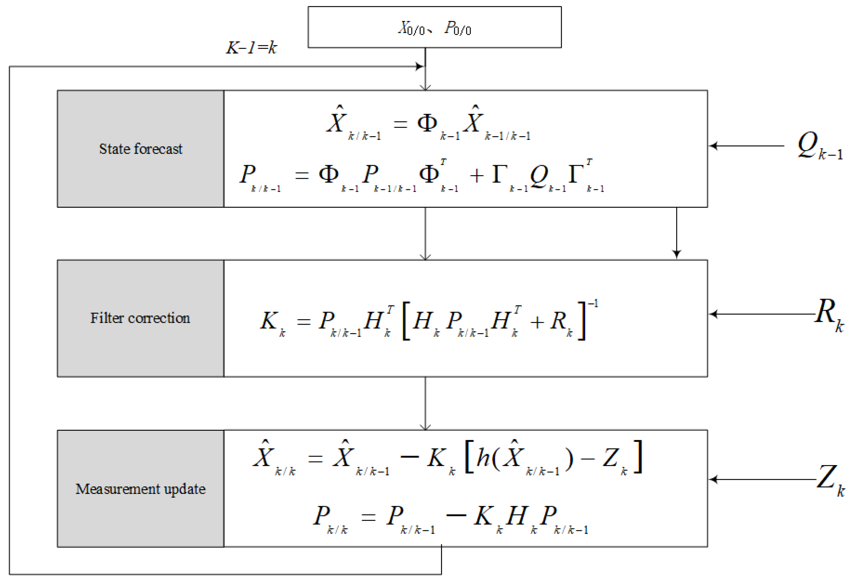
4.1. Extended Kalman Filters

KF is a recursive form of minimum variance estimation, and its working principle is as follows [37]:

Assuming the existing discrete system equation is

$$\{\begin{array}{l}{X}_k={\mathrm{\Phi }}_{k-1}{X}_{k-1}+{\mathrm{\Gamma }}_{k-1}{W}_{k-1}\\ Z_k=H_k{X}_k+V_{k-1}\end{array}$$

(36)

The calculation process $X_k$ of the optimal estimation ${\widehat{X}}_k$ of the system state can be divided into the following three steps:

• State forecast

The state and variance matrix of the next time $t_k$ system are estimated by the optimal estimation ${\widehat{X}}_{k-1/k-1}$ of the time system $t_{k-1}$ and the variance matrix $P_{k-1/k-1}$, which can be expressed as ${\widehat{X}}_{k/k-1}$ and $P_{k/k-1}$.

$${\widehat{X}}_{k/k-1}={\mathrm{\Phi }}_{k-1}{\widehat{X}}_{k-1/k-1}$$

(37)

$$P_{k/k-1}={\mathrm{\Phi }}_{k-1}{P}_{k-1/k-1}{\mathrm{\Phi }}_{k-1}^T+Q_{k-1}$$

(38)

2.

Filter correction

According to the variance matrix of the prediction estimate, the Kalman gain matrix is calculated.

$$K_k=P_{k/k-1}{H}_k^T{\left[H_k^{}{P}_{k/k-1}{H}_k^T+R_k\right]}^{-1}$$

(39)

3.

Measurement update

According to the observed values, the Kalman gain matrix is used to update the estimated state and the variance matrix to obtain an optimal estimate.

$${\widehat{X}}_{k/k}={\widehat{X}}_{k/k-1}-K_k\left[h({\widehat{X}}_{k/k-1})-Z_k\right]$$

(40)

$$P_{k/k}=P_{k/k-1}-K_k{H}_k{P}_{k/k-1}$$

(41)

The core content of the Kalman filter can be summarized into the aforementioned formulas. The specific workflow is shown in Figure 7.

A nonlinear continuous system, which needed to be transformed into a linear discrete system to use the aforementioned filtering methods, was adopted in the present study. First, according to Equation (35), the system was linearized, the high-order term was discarded, and the first-order term was taken to obtain [38]:

$$\{\begin{array}{l}\dot{X}\left(t\right)=F(\widehat{X})X\left(t\right)+Gw\left(t\right)\\ Z\left(t\right)=H(\widehat{X})X\left(t\right)+v\left(t\right)\end{array}$$

(42)

$$\{\begin{array}{l}F(X)=\frac{\partial f\left(X\right)}{\partial X}\\ H(X)=\frac{\partial h\left(X\right)}{\partial X}\end{array}$$

(43)

where $F(\widehat{X})$ and $H(\widehat{X})$ represent the linear system matrix and the measurement matrix at the state estimation value $\widehat{X}$. Through Taylor expansion, the linearized result was discretized to obtain the state transition matrix:

$$\mathrm{\Phi }(\widehat{X},t)=e^{F(\widehat{X})t}=I+F(\widehat{X})t+\frac{{\left[F(\widehat{X})\right]}^2}{2!}+\cdots \frac{{\left[F(\widehat{X})\right]}^n}{n!}\cdots$$

(44)

Taking the first two terms and assuming that the time step is $T_s$, the state transition matrix ${\mathrm{\Phi }}_{k-1}$ from the optimal estimator ${\widehat{X}}_{k-1}$ at time $k-1$ to time $k$ could be obtained:

$${\mathrm{\Phi }}_{k-1}=I+A(k-1)T_s$$

(45)

where $A(k-1)$ is the Jacobi matrix of the system matrix $F(\widehat{X})$. According to (43), $H_k$ can be obtained as:

$$\begin{array}{cc}{H}_k\hfill & ={\frac{\partial h\left[X_k,k-1\right]}{\partial X_k^T}|}_{X_k=X_k^n}\hfill \\ \hfill & =\left[\begin{array}{llll}{h}_{11}\hfill & 0\hfill & h_{13}\hfill & 0\hfill \\ h_{21}\hfill & 0\hfill & h_{23}\hfill & 0\hfill \end{array}\right]\hfill \end{array}$$

(46)

where:

$$\{\begin{array}{l}{h}_{11}=\frac{-L_{21}\sin x_1\cos x_3+L_{22}\cos x_1+L_{23}\sin x_1\sin x_3}{\sqrt{1-W^2}}\\ h_{13}=\frac{-L_{21}\sin x_3\cos x_1-L_{23}\cos x_1\cos x_3}{\sqrt{1-W^2}}\\ h_{21}=\frac{\left(-\frac{L_{32}}{{\cos }^2{x}_1}\right)U-\left(\frac{L_{12}}{{\cos }^2{x}_1}\right)V}{V^2+U^2}\\ h_{23}=\frac{(L_{33}\cos x_3+L_{31}\sin x_3)U-(-L_{11}\sin x_3-L_{13}\cos x_3)V}{V^2+U^2}\end{array}$$

(47)

$$\{\begin{array}{l}U=L_{11}\cos x_3+L_{12}\tan x_1-L_{13}\sin x_3\\ V=L_{33}\sin x_3-L_{31}\cos x_3-L_{32}\tan x_1\\ W=L_{21}\cos x_1\cos x_3+L_{22}\sin x_1-L_{23}\sin x_3\cos x_1\end{array}$$

(48)

The aforementioned state transition matrix ${\mathrm{\Phi }}_{k-1}$ and measurement matrix $H_k$ were brought into the filter to complete the filtering. So far, the filtering model has been established.

4.2. Iterated Extended Kalman Filter

In the process of linearization, the EKF ignores the second-order and higher-order terms, which belong to suboptimal estimation. When the system has strong nonlinearity, large errors will occur. Thus, to improve the accuracy of the algorithm, the IEKF was adopted. The IEKF is a combination of the extended Kalman filter and the iterative filter [39]. In the state prediction, the prediction formula of the extended Kalman filter is still used. In the state updating, the algorithm expands the observed values by means of the Taylor series, which are taken into Equation (40), and iteratively updates Equations (40) and (41) to reduce the state estimation error of the Kalman filter.

As the best estimate before the measured value at time k is obtained, the extended Kalman filter linearizes $h(X_k)$ at ${\widehat{X}}_k^{-}$ (superscript “−” indicates prior estimation). However, after the k-th filtering, a new and better estimated value ${\widehat{X}}_k^{+}$ at time k (superscript “+” means posterior estimation) could be obtained. If $h(X_k)$ is expanded again at ${\widehat{X}}_k^{+}$, a better posterior estimation can be obtained. Accordingly, several iterations were conducted to reduce estimation errors.

First, the observation equation $h_k=\left(X_k,V_k\right)$ was expanded by means of Taylor at ${\widehat{X}}_k^{+}$:

$$\begin{array}{cc}h\left(X_k,V_k\right)\hfill & =h\left({\widehat{X}}_k^{+},0\right)+\frac{\partial h}{\partial X}/\left(X_k-{\widehat{X}}_k^{+}\right)+\frac{\partial h}{\partial V}/V_k\hfill \\ \hfill & =h\left({\widehat{X}}_k^{+},0\right)+H_k\left(X_k-{\widehat{X}}_k^{+}\right)+M_k{V}_k\hfill \end{array}$$

(49)

Ignoring higher-order small quantities, the linearization result of the observation equation can be obtained:

$$h\left(X_k,V_k\right)=h\left({\widehat{X}}_k^{+}\right)+H_k\left(X_k-{\widehat{X}}^{+}\right)$$

(50)

The upper linearization result of the equation was taken at the prior estimate ${\widehat{X}}_k^{-}$ to replace $h\left({\widehat{X}}_{k|k-1}\right)$ in Equation (40), and the correction term in the state update equation could be obtained as follows:

$${\gamma }_k=Z_k-h\left({\widehat{X}}_k^{+}\right)-H_k\left({\widehat{X}}_k^{-}-{\widehat{X}}_k^{+}\right)$$

(51)

The state update equation is:

$${\widehat{X}}_{k,1}^{+}={\widehat{X}}_k^{-}+K_k\left[Z_k-h\left({\widehat{X}}_k^{+}\right)-H_k\left({\widehat{X}}_k^{-}-{\widehat{X}}_k^{+}\right)\right]$$

(52)

The IEKF algorithm was obtained by repeating the described cycle for many times as follows:

$$\begin{array}{l}{H}_{k,i}={\frac{\partial h}{\partial X}|}_{{\widehat{X}}_{k,i}^{+}}\\ K_{k,i}=P_k^{-}{H}_{k,i}^T{\left(H_{k,i}{P}_k^{-}{H}_{k,i}^T+M_k{R}_k{M}_k^T\right)}^{-1}\\ P_{k,i+1}^{+}=\left(I-K_{k,i}{H}_{k,i}\right)P_k^{-}\\ {\widehat{X}}_{k,i+1}^{+}={\widehat{X}}^{-}+K_{k,i}\left[Z_k-h\left({\widehat{X}}_{k,i}^{+}\right)-H_{k,i}\left({\widehat{X}}_k^{-}-{\widehat{X}}_{k,i}^{+}\right)\right]\end{array}$$

(53)

i represents the number of iterations, and the linearization error could be reduced by setting different iterations.

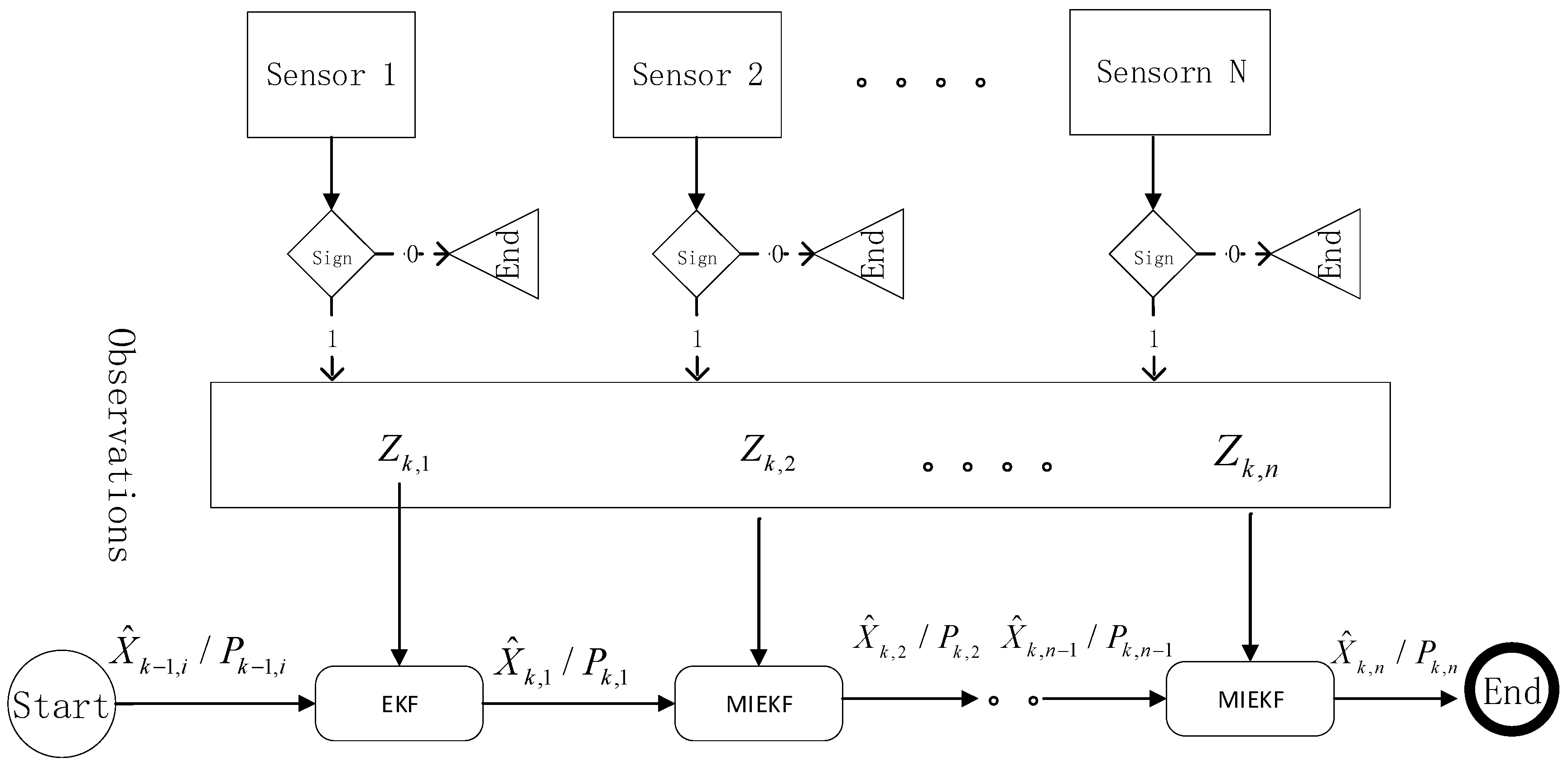
4.3. Multivariate Iterated Extended Kalman Filter

The MIEKF is inspired by the IEKF and was proposed in order to make full use of all the observations at the same time as well as the known error distribution information. The aim of the IEKF is to compensate for the nonlinear error of the EKF. The basic idea is that the filtered posterior estimate ${\widehat{X}}_k^{+}$ is better than the prior estimate ${\widehat{X}}_k^{-}$, and the errors caused by the linearization process can be reduced through continuous expansion and iteration at ${\widehat{X}}_k^{+}$. In the process of iteration, the observation information used by the IEKF is unchanged. As such, the method can only make up for the errors caused by the nonlinearity of the system, but it cannot reduce the errors caused by the observation noise of the system itself. The MIEKF proposed in the present study can make full use of the known noise distribution information of different sensors and iterate the observation values obtained by different sensors at the same time to reduce the errors caused by the observation noise. The specific process is as follows:

Assume that n observations are expressed as $Z_{k,i}$ at time k, and the observation noise matrix is known as $R_{k,i}$. One of the observations is used to perform the standard EKF, and the posterior estimation value ${\widehat{X}}_{k,1}^{+}$ is obtained by filtering. The iterative process is as follows:

First, according to Equation (49), $h_k=\left(X_k,V_k\right)$ will be expanded at ${\widehat{X}}_{k,i}^{+}$ (i represents the number of iterations), ignoring the high-order small quantity, and the linearization result will be obtained by taking the value at the prior estimation ${\widehat{X}}_k^{-}$:

$$h\left(X_k,V_k\right)=h\left({\widehat{X}}_{k,i}^{+}\right)+H_{k,i}\left(X_k-{\widehat{X}}_{k,i}^{+}\right)$$

(54)

where $H_{k,i}$ represents the Jacobi matrix of $h_k$ at ${\widehat{X}}_{k,i}^{+}$:

$$H_{k,i}={\frac{\partial h}{\partial X}|}_{{\widehat{X}}_{k,i}^{+}}$$

(55)

By replacing $h\left(\widehat{X}(k|k-1)\right)$ in Equation (40) with the result of upper linearization (54), and updating the observed values at the same time, the correction term in the state update equation could be obtained as follows:

$${\gamma }_{k,i}=Z_{k,i+1}-h\left({\widehat{X}}_{k,i}^{+}\right)-H_{k,i}\left(X_k-{\widehat{X}}_{k,i}^{+}\right)$$

(56)

where $Z_{k,i}$ represents the ith observation at time k. Thus, the following multivariate iterative extended Kalman filtering (MIEKF) algorithm could be obtained:

$$\begin{array}{l}{H}_{k,i}={\frac{\partial h}{\partial X}|}_{{\widehat{X}}_{k,i}^{+}}\\ K_{k,i}=P_k^{-}{H}_{k,i}^T{\left(H_{k,i}{P}_k^{-}{H}_{k,i}^T+M_k{R}_k{M}_k^T\right)}^{-1}\\ P_{k,i+1}^{+}=\left(I-K_{k,i}{H}_{k,i}\right)P_k^{-}\\ {\widehat{X}}_{k,i+1}^{+}={\widehat{X}}^{-}+K_{k,i}\left[Z_{k,i+1}-h\left({\widehat{X}}_{k,i}^{+}\right)-H_{k,i}\left({\widehat{X}}_k^{-}-{\widehat{X}}_{k,i}^{+}\right)\right]\end{array}$$

(57)

Combined with the object of the present study, the following processing flow could be obtained:

According to Figure 8, there will be N sensors to detect the target at time k. Because the target may not appear in all fields of view of the sensors, the sensor unit will output the Sign information while outputting the body LOS angle information of the target. Unless the sensor detects the target, Sign = 1; otherwise, Sign = 0. According to the Sign signal, the effective observation information is extracted to form the observation set Observation. The algorithm starts to use the first effective observation $Z_{k,1}$, combines the state quantity ${\widehat{X}}_{k-1,i}$ at time k − 1 and the covariance information $P_{k-1,i}$ of the system, and uses the standard extended Kalman filter to obtain the posterior estimation ${\widehat{X}}_{k,1}$. Subsequently, the next observation is extracted from the set of valid observations, and the multivariate iterative extended Kalman filter is used in combination with Equation (57) until all valid observations in the set are used up.

The MIEKF makes use of the non-equivalent observations with known error distribution at the same time and iterates multiple observations according to the covariance matrix of observation noise, thereby achieving the purpose of reducing the observation noise and effectively improving the precision of estimation information.

5. Numerical Simulations

In this paper, a 6-DOF trajectory simulation model was established based on previous research [36], and a flight trajectory was designed. The seeker model was embedded in the simulation model, and the actual measurement process of the seeker was simulated. The simulated measurement values of each channel of the array sensor were generated, and noise was added as the measurement result of the sensor. Through a ballistic analysis method, the advantages and disadvantages of the designed sensor array layout were examined, and the correctness of the guidance information extraction algorithm was verified.

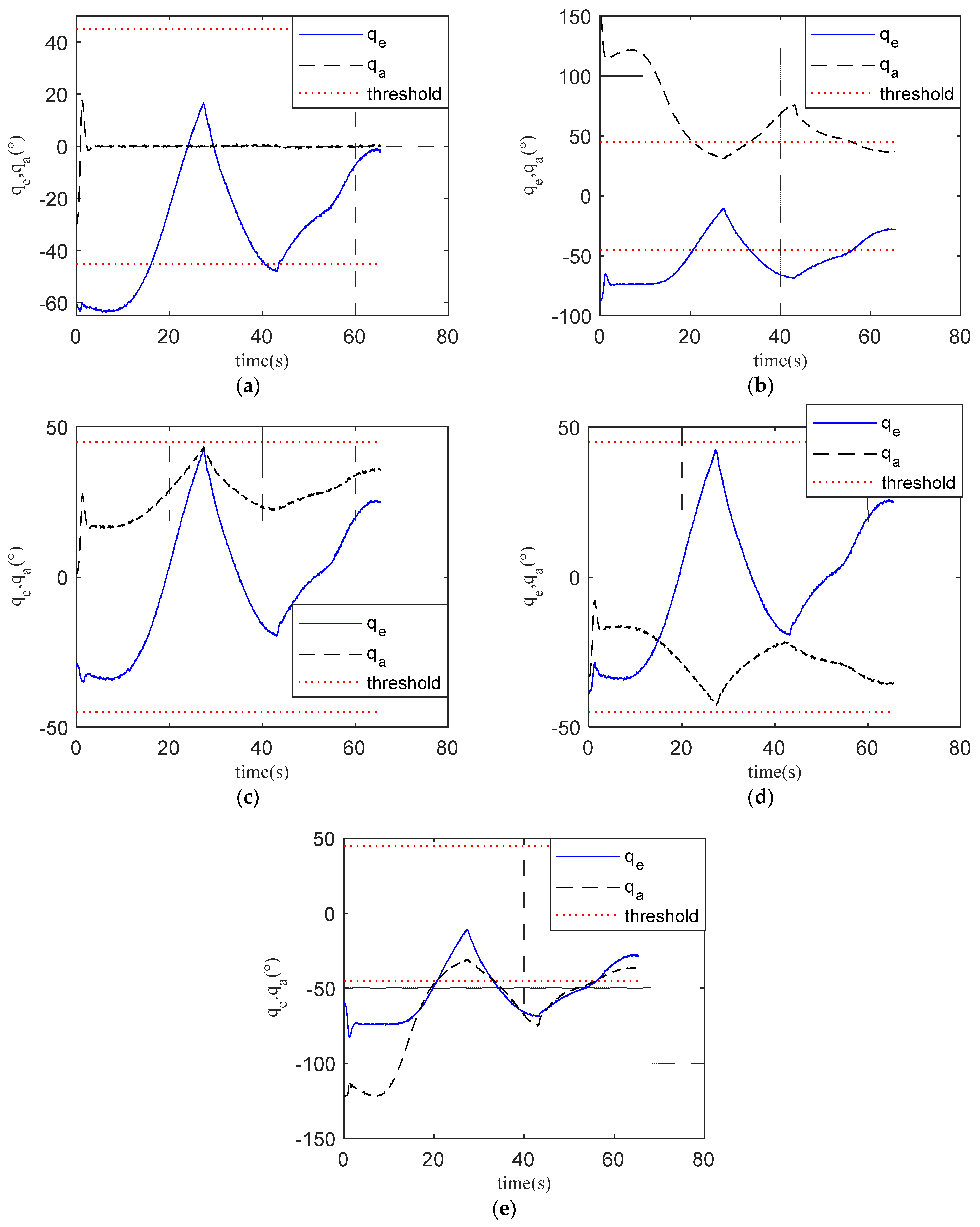
5.1. Generation of Measurement Data

The 6-DOF ballistic simulation model can give the missile’s altitude, velocity, position, and target’s position. According to the above information, the expression of the position of the target relative to the missile in the BCS B can be obtained. Combined with the angle between the sensors and the missile given in Section 2.1, the expression can be converted into SCS $I$. Then, the target LOS azimuth angle $q_a$ and target LOS azimuth angle $q_e$ of the target in SCS $I$ can be obtained. The measurement noise with the standard deviation of 0.2236°—that is, the variance of 0.05—was added as the measurement result. The research object of this paper is the infrared sensor. As mentioned in Section 2, the focus of the present study is guidance information extraction methods. So, it is assumed that the detection distance is far enough in the simulation. Under the assumption above, the measurement data of five sensors are simulated, as shown in Figure 9.

In Figure 9, the blue curve $q_e$ represents the target LOS altitude angle, and the black curve $q_a$ represents the target LOS azimuth angle detected by the sensor. As mentioned in Section 2, the FOV angle of the sensor is 45°. The red curve threshold represents the sensor FOV boundary. The target appeared within the sensor FOV range only when the line-of-sight (LOS) angle was within the threshold interval. When the sensor had an output value, Sign = 1; otherwise, Sign = 0, which means that the sensor had not detected the target. Measurement noise depends on the measurement error of the seeker sensor. According to the sensor noise designed in the simulation, the observed noise matrix can be obtained as:

$$R_k=\left[\begin{array}{cc}0.05/{57.3}^2& 0\\ 0& 0.05/{57.3}^2\end{array}\right]$$

(58)

According to the filter model, the system disturbance comes from the errors of altitude, position, and velocity provided by the missile. It depends on the accuracy of the inertial measurement unit installed on the missile. Thus, once the device is determined, the system noise matrix can be identified as constant. In the simulation, the accuracy of the inertial measurement unit is high, and the system error caused by it is small. The variance of the LOS angle error is 0.001, and the variance of the LOS angle rate is 0.3 [40]. The system noise matrix can be obtained as follows:

$$Q_k=\left[\begin{array}{cccc}0.001/{57.3}^2& 0& 0& 0\\ 0& 0.3/{57.3}^2& 0& 0\\ 0& 0& 0.001/{57.3}^2& 0\\ 0& 0& 0& 0.3/{57.3}^2\end{array}\right]$$

(59)

The initial covariance matrix depends on the accuracy of the initial state quantity. The more accurate the state quantity, the smaller the initial covariance matrix. In the simulation, the initial state is more accurate, so the corresponding covariance is small.

$$P\left(0/0\right)=\left[\begin{array}{cccc}-5.7\times {10}^{-6}& 0& 0& 0\\ 0& -8.4\times {10}^{-6}& 0& 0\\ 0& 0& -4.2\times {10}^{-6}& 0\\ 0& 0& 0& -5.8\times {10}^{-6}\end{array}\right]$$

(60)

The missile is set to be launched from the ground towards the target in the simulation. Therefore, the initial LOS angle $\epsilon$, $\eta$ and LOS angle rate $d\epsilon$, $d\eta$ are 0.

$$\widehat{X}(0/0)={[\begin{array}{cccc}0& 0& 0& 0\end{array}]}^T$$

(61)

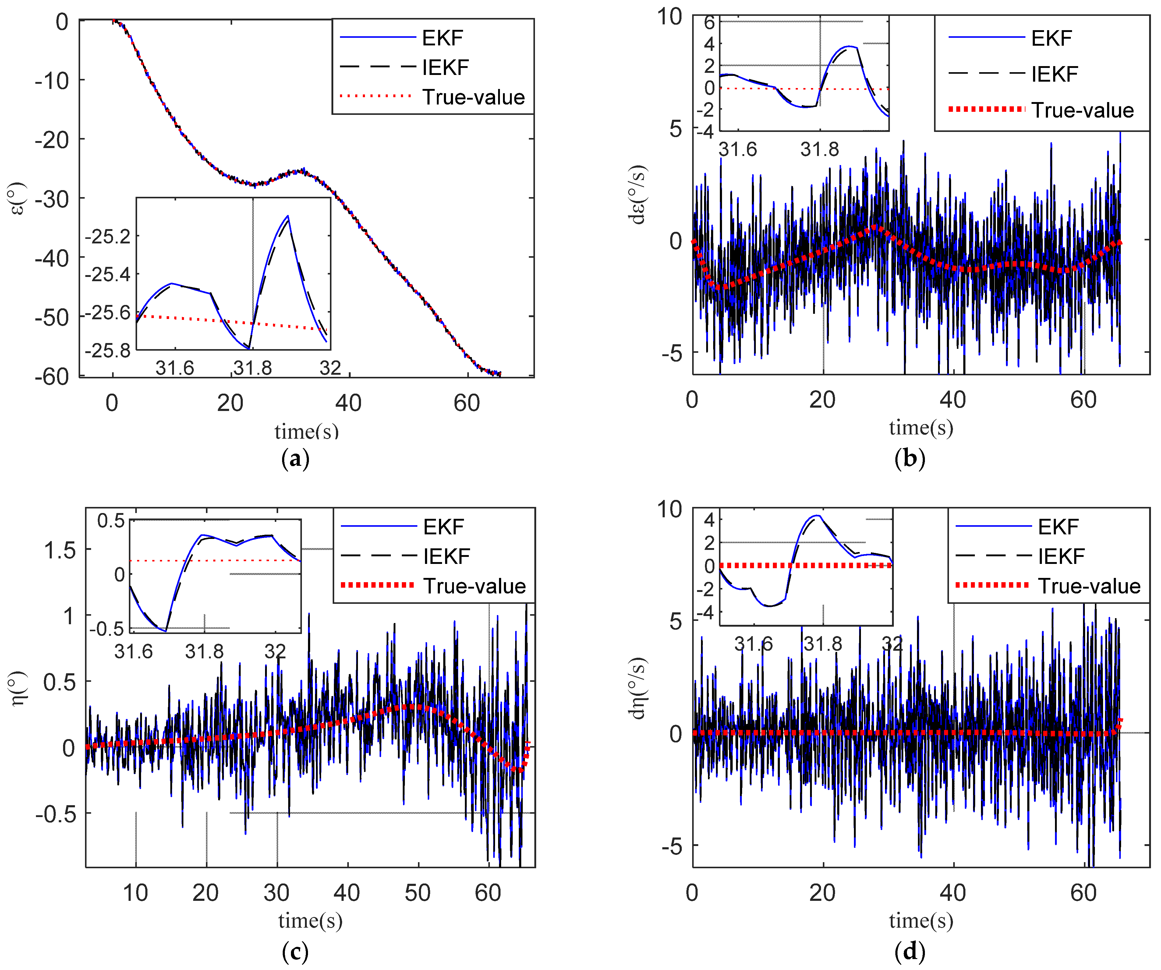
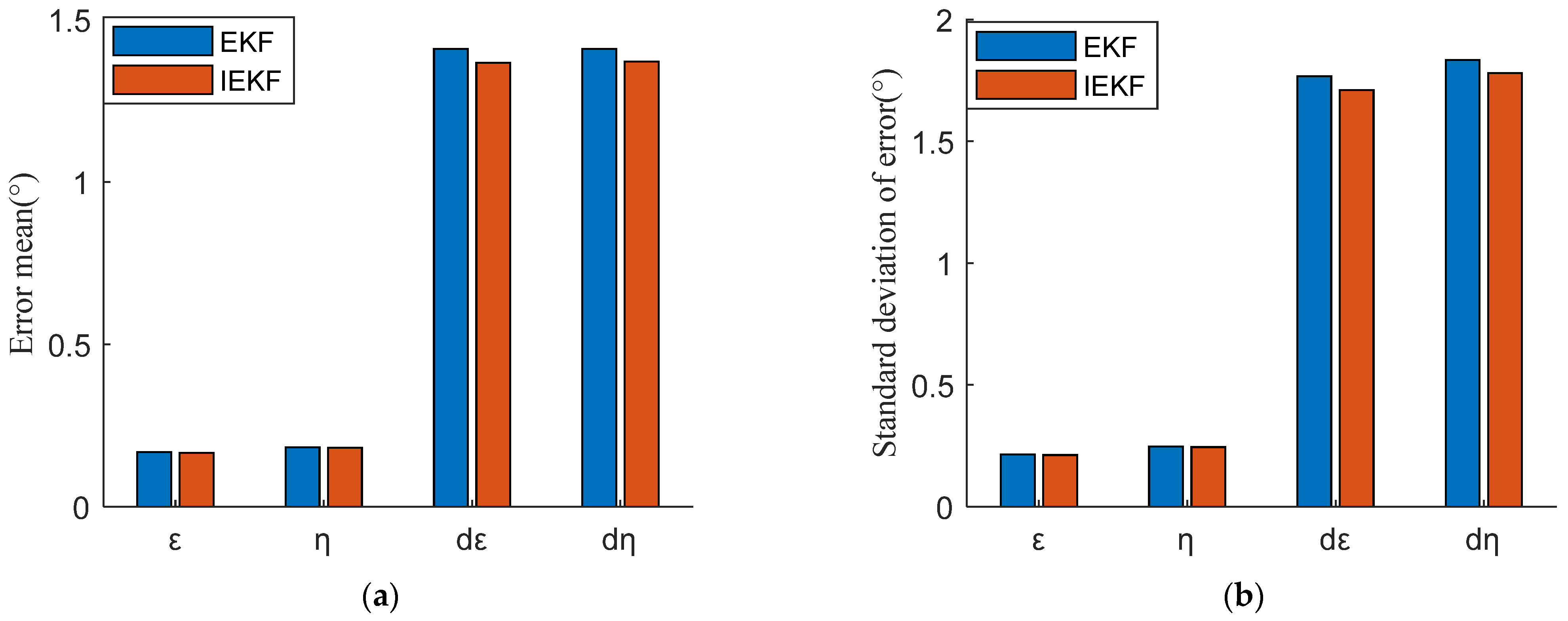
5.2. Results of IKEF and EKF

For the seeker with a single sensor, based on the measurement results of Sensor 1, the EKF and IEKF were used to extract the guidance information without considering the FOV constraint. Under the condition of setting the number of iterations times to five, the results are as follows.

The EKF method has been successfully applied in reference [31,40], so the results obtained by EKF are used as a comparative reference in this paper. As can be seen from Figure 10, both the EKF and the IEKF could be effectively used for guidance information extraction, but the filtered results were noisy. The LOS angle ε and η and LOS angle rate dε and dη obtained by the two methods are very close. In order to compare the accuracy, the error means and standard deviations of the error of the two methods are given below.

Table 2. The error means and standard deviations of error of EKF and IEKF.

Filter	Error Mean				Standard Deviation of Error
	ε [°]	η [°]	dε [°/s]	dη [°/s]	ε [°]	η [°]	dε [°/s]	dη [°/s]
EKF	0.1685	0.1833	1.4103	1.4102	0.2148	0.2471	1.7671	1.8347
IEKF	0.1662	0.1818	1.3667	1.3704	0.2121	0.2446	1.7103	1.7808

and Figure 11 show the mean error and standard deviation of error obtained by the difference between filtering results and truth value. It can be seen from Figure 11 that the LOS angle and LOS angle rate error obtained by IEKF are smaller than those obtained by EKF. The error mean is used as the accuracy evaluation index. According to Table 2, it can be calculated that IKEF method can improve the accuracy of LOS angle extraction by less than 5%, and the accuracy of LOS angle rate extraction by less than 5%. At the same time, it can be seen from the error standard deviation that IEKF does not decrease effectively compared with EKF, which means that the error distribution of IEKF results does not decrease significantly. This can also be verified in Figure 10. Such findings could be attributed to the nonlinearity of the system being weak, and the simulation time step being small. So, the IEKF did not significantly reduce the nonlinear error on the basis of the EKF. However, the iterative method will notably increase the amount of computation in multiples, and thus, the IEKF should not be adopted when there are no obvious advantages.

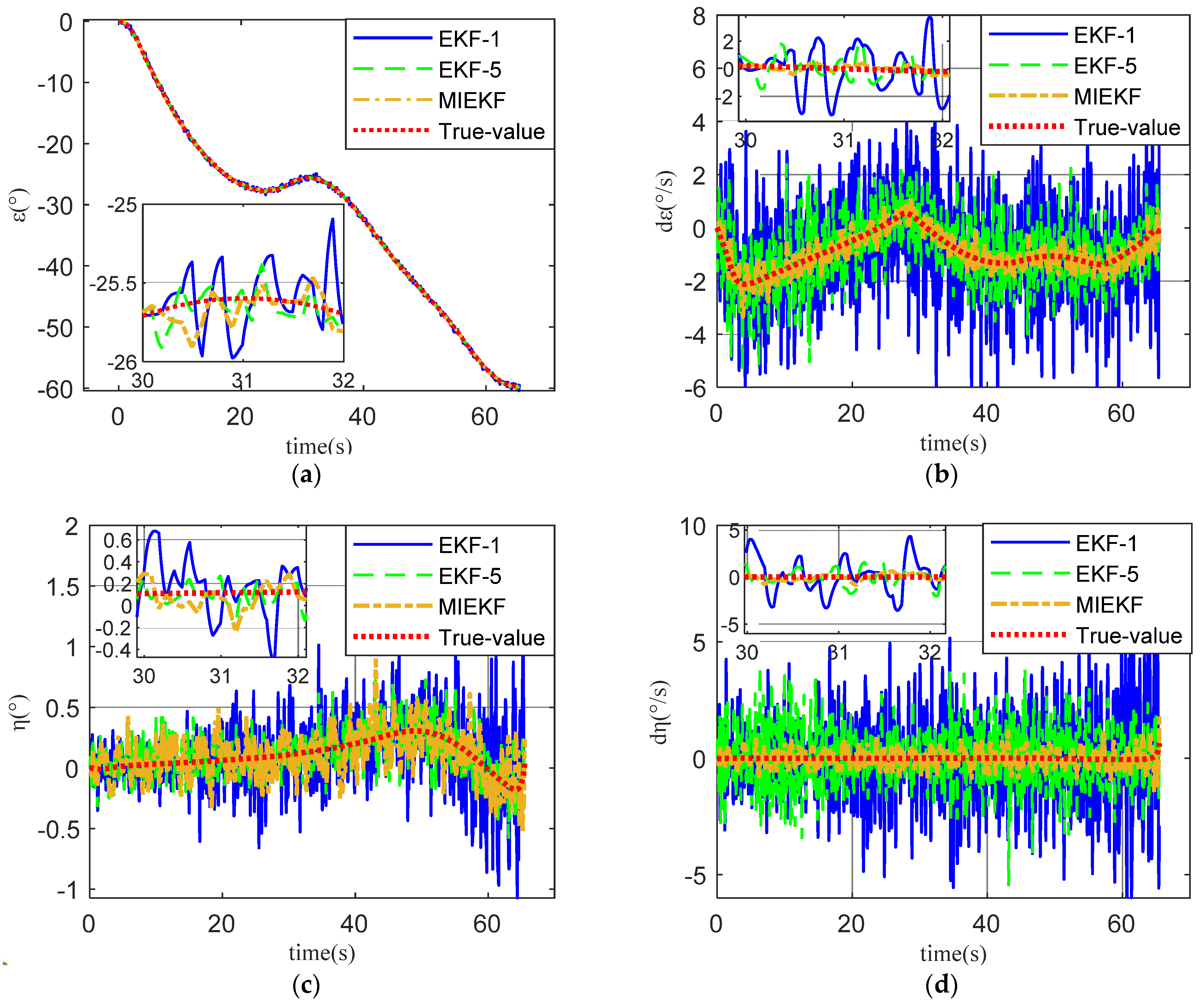
5.3. Results of MIKEF and EKF

The simulation results above are all based on monocular seekers. Additionally, the proposed rectangular FOV sensors array seeker was simulated and analyzed, applying EKF and MIEKF, and the results are as follows.

The EKF-1 curve in Figure 12 shows the results obtained by the EKF filtering method based on monocular sensor 1. The EKF-5 curve shows the results obtained by filtering with the EKF method based on multi-sensor seekers—that is, without considering the error distribution of sensors in each channel, the measured results were normalized to obtain the average value, and the extended Kalman filter (EKF) was used for filtering. The MIEKF curve shows the results obtained by using the MIEKF filtering method based on multi-sensor seekers after normalization and considering error distribution. Figure 12 shows that the noise levels of curve EKF-5 and curve MIEKF after filtering were obviously lower than that of curve EKF-1, indicating that the increased measurement information could effectively improve the data accuracy. It can be seen from Figure 12a,c that the noise magnitude of EKF-5 and MIEKF is similar in LOS angle estimation. As can be seen from Figure 12b,d, compared with the EKF-5, the MIEKF had a significant effect in terms of reducing noise in the process of LOS angle rate estimation, effectively improving data accuracy. The error means and standard deviations of the error of the three methods are given below for further analysis.

Table 3. The error means and standard deviations of error of EKF-1, EKF-5 and MIEKF.

Filter	Error Mean				Standard Deviation of Error
	ε [°]	η [°]	dε [°/s]	dη [°/s]	ε [°]	η [°]	dε [°/s]	dη [°/s]
EKF-1	0.1685	0.1833	1.4103	1.4102	0.2148	0.2471	1.7671	1.8347
EKF-5	0.0990	0.1132	0.7928	0.9491	0.1276	0.1439	1.0115	1.2013
MIEKF	0.1039	0.1256	0.2652	0.2883	0.1325	0.1572	0.3295	0.3612

and Figure 13 show the mean errors and standard deviations of error obtained by the difference between filtering results and truth value. Additionally, EKF-1 was used as the comparison reference, and the error mean was used as the accuracy index. Table 3 shows that EKF-5 improves the accuracy of LOS angle ε and η by 41% and 38%, respectively, and improves the accuracy of LOS angle rate dε and dη by 43% and 32%, respectively. MIEKF improves the accuracy of LOS angle ε and η by 38% and 31%, respectively, and improves the accuracy of LOS angle rate dε and dη by 81% and 79%, respectively. According to the above results, it can be concluded that MIEKF has a significant effect on improving the accuracy of the LOS angle rate, and the improvement of LOS angle accuracy mainly depends on the increase of observation quantity. Meanwhile, compared with EKF-1, the standard deviation of MIEKF’s LOS angle error is reduced by nearly 40%, which means that the LOS angle distribution obtained by MIEKF is reduced. This can also be verified in Figure 12a,c. The standard deviation of MIEKF’s LOS angle rate error is reduced by nearly 80%. As can be seen from Figure 12b,d, compared with the EKF, the MIEKF had a significant effect in terms of reducing noise in the process of LOS angle rate extraction, effectively improving data accuracy. Furthermore, the LOS angle rate is often used in the guidance process. Overall, the results show that the MIEKF proposed in this study, combined with the array sensor seeker, can effectively improve the data precision in the process of guidance information extraction.

Figure 14 shows the number of effective sensors under a monocular seeker and multi-eye seeker. It can be seen that the multi-eye seeker could ensure that at least two sensors could capture the target at the same time, and all five sensors could capture the target at the peak, regardless of the sensor detection distance. However, the monocular seeker would lose the target in the flight process. To avoid this situation, the constraint term is usually added into the design of the guidance law, which would limit the maneuverability of the missile.

Figure 15 shows the target trajectory distribution in the seeker’s FOV during the whole flight process. It can be seen that when the missile had just launched, the target position was far from the y-axis due to the influence of the initial altitude angle. With the stabilization of the altitude, the target position was distributed near the y-axis as expected. According to Figure 14, during the whole flight process, the target was basically within the FOV of Sensor No. 1, but at about 41 s, the target was out of the FOV range of Sensor No.1 due to missile maneuvering. Here, the monocular sensor would lose the target, while the array sensor seeker still had two sensors that could detect the target, which could ensure that the target was always in the FOV during the flight process.

6. Conclusions

The research object of the this was the strapdown multi-view surface array seeker. The aim was to expand the FOV and improve the precision of guidance information by means of array sensors. The main aspects of the study include:

(1)

The field distribution of the circular FOV sensor and the rectangular FOV sensor in the +-shaped layout and the X-shaped layout were explored. The FOV after the array superposition was characterized by the FOV of the central sensor, and the equivalent FOV of the monocular seeker was obtained. The results show that the FOV angle is enlarged to 75.1° and 63.8° in +-shape and X-shape layout when five circular FOV sensors with 45° × 45° FOV angle are used. The FOV angle is enlarged to 70.5° × 90° and 72° × 75° in +-shape and X-shape layout when five rectangular FOV sensors with 45°FOV angle are used. Although the +-shape layout has a larger FOV angle, the X-shape layout has better FOV coverage. In an X-shape layout, there are at least two sensors around the y-axis to provide coverage. In the central area, coverage can be up to five sensors, which is an ideal sensor layout.

(2)

In order to solve the problem that the number of observations changes during the observation process, the measurement results $q_e^i$, $q_a^i$ and noise errors $v_{1i}$, $v_{2i}$ of surface array sensors were normalized and characterized in the FOV of the central sensor. The equivalent observations $q_{ei}$, $q_{ai}$ and the corresponding error distributions $w_{1i}$, $w_{2i}$ were obtained. A model of guidance information extraction (28) and (34) was established based on the observations and error distributions.

(3)

For the established continuous nonlinear model, the EKF was used for processing. The IEKF was adopted for comparative analysis to overcome the nonlinear error in the filtering process. However, the simulation results show that, compared with EKF, IEKF improves the accuracy of the LOS angle and LOS angle rate by less than 5%. This means that the nonlinear error was not the main error source. In order to make full use of the observed values of the array sensors, improve the filtering quality, and reduce the noise error, the MIEKF was proposed. The simulation results show that the MIEKF can improve the estimation accuracy of LOS angle ε and η by at least 30% and the estimation accuracy of LOS angle rate dε and dη by nearly 80% compared with EKF. So, the MIEKF proposed in this paper is helpful for improving the accuracy of guidance information.

The sensor is being tested at present. In the future, the measurement error distribution characteristics of the sensor will be studied, and the actual performance of the sensor and the uncertainty of the model parameters will be considered to test the robustness of the system. In the present study, only five sensor arrays based on the +-shaped layout and the X-shaped layout were investigated. The different numbers of sensors and performances of different layouts of array seekers were not compared and analyzed and therefore need to be investigated in future research.

References

1. Zuo, W.; Zhou, B.; Li, W. Analysis of Development of Multi-mode and compound Precision Guidance Technology. Air Space Def. 2019, 2, 44–52. [Google Scholar]
2. Lee, J.Y. Generalized Guidance Formulation for Impact Angle Interception with Physical Constraints. Aerospace 2021, 8, 307. [Google Scholar]
3. Park, B.G.; Kwon, H.H.; Kim, Y.H. Composite Guidance Scheme for Impact Angle Control Against a Nonmaneuvering Moving Target. J. Guid. Control. Dyn. 2016, 39, 1129–1136. [Google Scholar] [CrossRef]
4. Tekin, R.; Erer, K.S. Switched-Gain Guidance for Impact Angle Control Under Physical Constraints. J. Guid. Control Dyn. 2015, 38, 205–216. [Google Scholar] [CrossRef]
5. Zhang, H.Q.; Tang, S.J.; Guo, J. A Two-Phased Guidance Law for Impact Angle Control with Seeker’s Field-of-View Limit. Int. J. Aerosp. Eng. 2018, 2018, 740363. [Google Scholar] [CrossRef]
6. Park, B.G.; Kim, T.H.; Tahk, M.J. Biased PNG With Terminal-Angle Constraint for Intercepting Nonmaneuvering Targets Under Physical Constraints. IEEE Trans. Aerosp. Electron. Syst. 2017, 53, 1562–1572. [Google Scholar] [CrossRef]
7. Wang, Z. Field-of-View Constrained Impact Time Control Guidance via Time-Varying Sliding Mode Control. Aerospace 2021, 8, 251. [Google Scholar]
8. Singh, N.K.; Hota, S. Moving Target Interception Guidance Law for Any Impact Angle with Field-of-View Constraint. AIAA Scitech 2021 Forum 2021, 1462. [Google Scholar] [CrossRef]
9. Qian, S.K.; Yang, Q.H.; Geng, L.N. SDRE Based Impact Angle Control Guidance Law Considering Seeker’s Field-of-View Limit. In Proceedings of the Chinese Guidance, Navigation and Control Conference, Nanjing, China, 12–14 August 2016. [Google Scholar]
10. Lee, S.; Ann, S.; Cho, N.; Kim, Y. Capturability of Impact-Angle Control Composite Guidance Law Considering Field-of-View Limit. IEEE Trans. Aerosp. Electron. Syst. 2020, 56, 1077–1093. [Google Scholar] [CrossRef]
11. Ma, S.; Wang, Z.Y.; Wang, X.G. Three-Dimensional Impact Time Control Guidance Considering Field-of-View Constraint and Velocity Variation. Aerospace 2022, 9, 202. [Google Scholar] [CrossRef]
12. Zhao, B.; Xu, S.Y.; Guo, J.G. Integrated Strapdown Missile Guidance and Control Based on Neural Network Disturbance Observer. Aerosp. Sci. Technol. 2019, 84, 170–181. [Google Scholar] [CrossRef]
13. Sun, T.T. Research on the Key Technology of Strapdown; University of Chinese Academy of Sciences: Beijing, China, 2016. [Google Scholar]
14. Sun, X.T.; Luo, X.B.; Liu, Q.S. Application and Key Technologies of Guided Munition Based on Strapdown Seeker. J. Ordnance Equip. Eng. 2019, 40, 58–61. [Google Scholar]
15. Song, Y.F.; Hao, Q.; Cao, J. Research and development of foreign Wide-Field-of-View seeker based on artificial compound eye. Infrared Laser Eng. 2021, 51, 20210593. [Google Scholar]
16. Zhang, X.; Xu, Y.; Fu, K. Field of View Selection and Search Strategy Design for Infrared Imaging Seeker. Infrared Laser Eng. 2014, 43, 3866–3871. [Google Scholar]
17. Hu, J.T.; Huang, F.; Zhang, C. Research status of super resolution reconstruction based on compound-eye imaging technology. Laser Technol. 2015, 39, 492–496. [Google Scholar]
18. Cao, J.; Hao, Q.; Zhang, F.H. Research progress of bio-inspired retina-like imaging. Infrared Laser Eng. 2020, 49, 9–16. [Google Scholar]
19. Duparré, J.; Wippermann, F.; Dannberg, P. Artificial compound eye zoom camera. Bioinspirat. Biomim. 2008, 3, 046008. [Google Scholar] [CrossRef]
20. Duparré, J.; Wippermann, F.; Dannberg, P. Chirped arrays of refractive ellipsoidal microlenses for aberration correction under oblique incidence. Opt. Express 2005, 13, 10539–10551. [Google Scholar] [CrossRef]
21. Nakamura, T.; Horisaki, R.; Tanida, J. Computational superposition compound eye imaging for extended depth-of-field and field-of-view. Opt. Express 2012, 20, 27482–27495. [Google Scholar] [CrossRef]
22. Horisaki, R.; Tanida, J. Preconditioning for multidimensional TOMBO imaging. Opt. Lett. 2011, 36, 2071–2073. [Google Scholar] [CrossRef]
23. Zhai, Y.; Niu, J.; Liu, J. Bionic Artificial Compound Eyes Imaging System Based on Precision Engraving. In Proceedings of the 2021 IEEE 34th International Conference on Micro Electro Mechanical Systems, Gainesville, FL, USA, 25–29 January 2021. [Google Scholar]
24. Fan, Y. Design and Simulation of the Artificial Compound Eyes with Large Field of View; Tianjin University: Tianjin, China, 2013. [Google Scholar]
25. Song, L.P. Design of Distributed Full Strapdown Guidance Bomb Guidance Information Extraction and Guidance System; Harbin Institute of Technology: Harbin, China, 2019. [Google Scholar]
26. Jang, S.A.; Ryoo, C.K.; Choi, K. Guidance Algorithms for Tactical Missiles with Strapdown Seeker. In Proceedings of the 2008 SICE Annual Conference, Chofu, Japan, 20–22 August 2008. [Google Scholar]
27. Raj, K.D.; Ganesh, I.S. Estimation of Line-of-Sight Rate in a Homing Missile Guidance Loop Using Optimal Filters. In Proceedings of the International Conference on Communications, Melmaruvathur, India, 2–4 April 2015. [Google Scholar]
28. Hong, J.H.; Ryoo, C.K. Compensation of Parasitic Effect in Homing Loop with Strapdown Seeker via PID Control. In Proceedings of the International Conference on Informatics in Control, Vienna, Austria, 1–3 September 2014; Volume 1, pp. 711–717. [Google Scholar]
29. Liu, Y.; Tian, W.F.; Zhao, J.K. Line-of-Sight Angle Rate Reconstruction for Phased Array Strapdown Seeker. Adv. Mater. Res. 2013, 645, 196–201. [Google Scholar] [CrossRef]
30. Mi, W.; Shan, J.; Liu, Y. Adaptive Unscented Kalman Filter Based Line of Sight Rate for Strapdown Seeker. In Proceedings of the Chinese Automation Congress (CAC), Xian, China, 30 November–2 December 2018. [Google Scholar]
31. Vergez, P.L.; Mcclendon, J.R. Optimal control and estimation for strapdown seeker guidance of tactical missiles. J. Guid. Control Dyn. 2012, 5, 225–226. [Google Scholar] [CrossRef]
32. Zhang, Y.C.; Li, J.J.; Li, H.Y. Line of sight rate estimation of strapdown imaging seeker based on particle filter. In Proceedings of the 2010 3rd International Symposium on Systems and Control in Aeronautics and Astronautics, Harbin, China, 8–10 June 2010. [Google Scholar]
33. Lan, J.; Li, X.R. Nonlinear Estimation by Linear Estimation with Augmentation of Uncorrelated Conversion. In Proceedings of the 17th International Conference on Information Fusion, Salamanca, Spain, 7–10 July 2014. [Google Scholar]
34. Lan, J.; Li, X.R. Nonlinear Estimation by LMMSE-Based Estimation with Optimized Uncorrelated Augmentation. IEEE Trans. Signal Processing 2015, 63, 4270–4283. [Google Scholar] [CrossRef]
35. Lan, J.; Li, X.R. Multiple Conversions of Measurements for Nonlinear Estimation. IEEE Trans. Signal Processing 2017, 65, 4956–4970. [Google Scholar] [CrossRef]
36. Chen, K.J.; Liu, L.H.; Meng, Y.H. Launch Vehicle Flight Dynamics and Guidance; National Defense Industry Press: Beijing, China, 2014. [Google Scholar]
37. Bucy, R.; Joseph, P. Filtering for Stochastic Processes with Applications to Guidance; John Wiley & Sons: New York, NY, USA, 1968. [Google Scholar]
38. Bellantoni, J.F.; Dodge, K.W. A square root formulation of the Kalman- Schmidt filter. AIAA J. 1967, 5, 1309–1314. [Google Scholar] [CrossRef]
39. Simon, D.J. Optimal State Estimation: Kalman, H Infinity, and Nonlinear Approaches; Wiley-Interscience: New York, NY, USA, 2006. [Google Scholar]
40. Yuan, Y.F. Research on Guidance and Control Technology for Strapdown Guided Munition; Beijing Institute of Technology: Beijing, China, 2014. [Google Scholar]
Figure 1. Sensor layout diagrams. (a) Left view of +-shaped layout. (b) Front view of +-shaped layout. (c) Left view of X-shaped layout. (d) Front view of X-shaped layout.
Aerospace 09 00373 g001
Figure 2. Back vision project images. (a) +-shaped layout. (b) X-shaped layout.
Aerospace 09 00373 g002
Figure 3. Transformation relationship between coordinate systems.
Aerospace 09 00373 g003
Figure 4. Sensor coordinate system.
Aerospace 09 00373 g004
Figure 5. Circular FOV sensor array overlay diagrams. (a) +-shaped layout. (b) X-shaped layout.
Aerospace 09 00373 g005
Figure 6. Rectangular FOV sensors array overlay diagrams. (a) +-shaped layout. (b) X-shaped layout.
Aerospace 09 00373 g006
Figure 7. Workflow of Kalman filter.
Aerospace 09 00373 g007
Figure 8. MIEKF filtering process.
Aerospace 09 00373 g008
Figure 9. The result of sensors measurement. (a) Sensor 1. (b) Sensor 2. (c) Sensor 3. (d) Sensor 4. (e) Sensor 5.
Aerospace 09 00373 g009
Figure 10. The results of EKF & IEKF. (a) Elevation of line-of-sight. (b) The rate of elevation of line-of-sight. (c) Azimuth of line-of-sight. (d) The rate of azimuth of line-of-sight.
Aerospace 09 00373 g010
Figure 11. The error of EKF and IEKF. (a) The mean error. (b) The standard deviation.
Aerospace 09 00373 g011
Figure 12. The results of EKF & MIEKF. (a) Elevation of line-of-sight. (b) The rate of elevation of line-of-sight. (c) Azimuth of line-of-sight. (d) The rate of azimuth of line-of-sight.
Aerospace 09 00373 g012
Figure 13. The error of EKF1, EKF5 and MIEKF. (a) The mean error. (b) The standard deviation.
Aerospace 09 00373 g013
Figure 14. The number of sensors which could detect the target.
Aerospace 09 00373 g014
Figure 15. The variation range of the field angle.
Aerospace 09 00373 g015