Fault-Tolerant Control for Hexacopter UAV Using Adaptive Algorithm with Severe Faults

Abstract

In this paper, a fault-tolerant control method is proposed for a hexacopter under uncertainties. The proposed method is based on adaptive-sliding-mode control (ASMC) and a control allocation scheme. First, a mathematical model of the hexacopter is employed with model uncertainties. Next, the control allocation strategy is combined with ASMC to handle actuator faults, which can distribute the virtual control signal to redundant actuators. A modified fault-tolerant control is proposed to overcome this virtual input saturation. Finally, the system stability is validated using the Lyapunov theory. The performance of the proposed method is compared with that of normal ASMC. The simulation results show that the suggested strategy can realize quicker compensation under faulty conditions.

1. Introduction

Unmanned aerial vehicles (UAVs) have drawn attention in recent decades due to their significant benefits in different domains, such as transportation, mapping, rescue, forest monitoring, agriculture, and the military. Hexacopters, a class of UAVs, have been intensively investigated owing to their properties, such as simple structures, economic efficiency, agility, and convenience of maintenance; thus, hexacopters are more widely used than other classes of UAV systems. Hexacopters have been expanded in different areas of application, including trajectory tracking, formation control, object detection and tracking, and fault-tolerant control (FTC). To increase the reliability and autonomy of UAV systems, fault-tolerant capabilities should be taken into account for handling the failures of actuators, system components, or sensors. FTC is classified as passive or active. Passive FTC approaches include robust controller designs that may not require fault diagnosis (FD) in a control system for accommodation. However, this method has a limited fault-tolerance capability. In order to improve fault-tolerance capability, active FTC approaches have been introduced. In these methods, FD is used to achieve knowledge of faults; the FTC is then integrated with FD information and a nominal controller to eliminate the fault effects. Thus, active FTC for a hexacopter system to address actuator faults has attracted significant research attention.

The issue of the FD strategy has been investigated in many articles. In [1], a Kalman-filter-based FD method was presented for actuator faults; the method yielded good experimental results. In [2], a linear parameter varying method was suggested for a quadcopter to estimate faults. A fault-tolerant controller based on fault estimation information was designed to accommodate faults. In [3,4], a Thau observer was proposed to estimate the time-varying fault in a quadcopter. However, the above approaches are not applicable to over-actuated systems such as hexarotors as they cannot identify faulty motors. Recently, an efficient method based on residual evaluation was investigated in [5]. This approach uses inertial sensor information to estimate the loss of control effectiveness (LoCE) in each actuator. However, this method cannot simultaneously estimate the magnitudes of all faulty actuators. To overcome this drawback, some methods have been investigated recently, which include the adaptive Kalman filter [6,7,8], the sliding mode observer [9], and the adaptive observer [10].

In the context of FTCs, several control techniques based on active schemes have been proposed to achieve fault-tolerance capability for UAV systems. The active FTC can integrate FD and FTC as a complete unit. In [11], an FTC based on a look-up table based on residual evaluation and pseudo-inverse control allocation was proposed. When one faulty motor is detected, a dual motor is used for the fault compensation. In [12], an FTC scheme based on an integral sliding mode and a fixed allocation matrix was proposed for an octorotor to handle disturbances and actuator faults; however, this method can only handle partial LoCE in the actuator. An intelligent FTC control strategy based on neural networks and fuzzy logic with potential simulation results was presented in [13]. As presented in [14], a fault-tolerant control and recovery scheme was implemented in an experimental study. A gain scheduling PID [1] control method was suggested for a quadrotor to handle actuator faults. The experiment shows that the suggested algorithm can adopt a LoCE of 18% for all actuators. Although the above studies presented potential results in the case of a partial LoCE in an actuator, the fault diagnosis module is not integrated into the nominal controller as a complete FTC system. To overcome this issue, several recent methods have been suggested for UAV systems to address actuator faults. In [15], a robust FTC based on self-scheduled control allocation was proposed for a hexacopter. The experiment involved different cases of LoCE in an actuator, and good performance was achieved. In a recent paper [16], a simple method was proposed to investigate partial and total LoCEs in actuators using gain-scheduling control with ${\mathrm{H}}_{\infty }$. In [17], an FTC based on an adaptive sliding mode, a disturbance observer, and residual evaluation was proposed to handle complete LoCE in one or two motors. However, the existing methods do not consider estimation errors from the allocation matrix and input saturation problems in controller design for the hexacopter model. Moreover, most of the current methods do not handle the unknown fault in one motor due to controllability problems.

In this article, an FTC technique based on an active scheme is designed for a hexacopter UAV to address actuator faults. The suggested approach was designed based on adaptive-sliding-mode control (ASMC) and adaptive control allocation. The objective of the proposed method is to utilize the control effectiveness of actuator redundancy. First, a mathematical model was proposed. Then, the combination of ASMC and an online control allocation scheme is investigated to stabilize the attitude and altitude system. Next, the adaptive SMC is modified to address the actuator saturation. Compared with the current methods used for hexacopters, the benefits of the suggested method and the major contributions of this study are as follows:

• The combination of adaptive SMC and online control allocation can provide good tracking performance in the presence of actuator faults and model uncertainties in the hexacopter model;
• The adaptive law is developed to overcome fault estimation error;
• The stability of the system is validated using Lyapunov theory;
• The proposed method is validated by simulation and is compared with a recent method [18]. The advantage of the proposed method is handling unknown complete faults in one motor. Moreover, the proposed method in this article considers the input saturation in controller design and self-reconfiguration through control allocation by using virtual control.

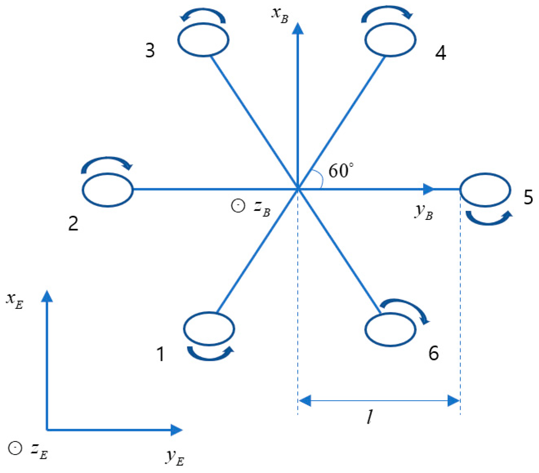
2. Mathematical Model of Hexacopter

Body frame B and inertial frame E are used to describe the dynamics of the hexacopter, as shown in Figure 1. With respect to the body frame, the X-Y plane is located at the surface, while the Z-axis is determined using the left-hand rule. In the quadcopter system, the center of gravity is located at the origin of the body frame.

The rotation matrix $R$ can be used for transformation from the inertial frame to the body frame as follows:

$$R=\left[\begin{array}{ccc}c\psi c\theta & c\psi s\theta s\varphi -s\psi c\varphi & c\psi s\theta c\varphi +s\psi c\varphi \\ s\psi c\theta & s\psi s\theta s\varphi +c\psi c\varphi & s\psi s\theta c\varphi -s\varphi c\psi \\ -s\theta & c\theta s\psi & c\theta c\varphi \end{array}\right]$$

(1)

where $s$ and $c$ denote sin and cos, respectively, and $\varphi ,\theta ,$$\psi$ denote Euler angles.

The hexacopter shown in Figure 1 includes three motors (1, 3, 5) rotating counterclockwise and the remaining motors rotating clockwise. According to the Newton–Euler formulation, the mathematical model of the hexacopter is as follows:

$$\left\{\begin{array}{l}m\ddot{r}=R\left[\begin{array}{l}0\\ 0\\ U_1\end{array}\right]-\left[\begin{array}{l}0\\ 0\\ mg\end{array}\right]-\dot{\mathrm{\Omega }}\times m\ddot{r}\\ I\ddot{\mathrm{\Omega }}=\left[\begin{array}{l}{U}_2\\ U_3\\ U_4\end{array}\right]-\dot{\mathrm{\Omega }}\times I\ddot{\mathrm{\Omega }}\end{array}\right.$$

(2)

where m is the mass of the hexacopter; $\mathrm{\Omega }$ is the attitude; g is the gravity; I is the inertia vector; r is the position in the inertial frame;

Assumed that the body rate can be approximated to Euler angle rate at a small angle change. Finally, the translational and rotational motions of the hexacopter can be obtained as [2]

$$\left\{\begin{array}{l}\ddot{x}=\left\{U_1(\cos \varphi sin\theta cos\psi +\sin \varphi \sin \psi )-K_x\dot{x}\right\}/m\\ \ddot{y}=\left\{U_1(\cos \varphi sin\theta sin\psi -\sin \varphi cos\psi )-K_y\dot{y}\right\}/m\\ \ddot{z}=-g+\left\{U_1(\cos \varphi cos\theta )-K_z\dot{z}\right\}/m\\ \ddot{\varphi }=\left(U_2+(I_2-I_3)\dot{\theta }\dot{\psi }-K_{\varphi }\dot{\varphi }\right)/I_1\\ \ddot{\theta }=\left(U_3+(I_3-I_1)\dot{\varphi }\dot{\psi }-K_{\theta }\dot{\theta }\right)/I_2\\ \ddot{\psi }=\left(U_4+(I_1-I_2)\dot{\varphi }\dot{\theta }-K_{\psi }\dot{\psi }\right)/I_3\end{array}\right.$$

(3)

where $I_1,I_2,I_3$ represent the moments of inertia of the quadcopter along the $x,y,z$ axes; $K_{\varphi },K_{\theta },K_{\psi },K_x,K_y$ represent the drag coefficients, and the virtual control inputs $(U_1,U_2,U_3,U_4)$ are developed by thrusts that are generated from six independent rotors. The relationship between the thrust $T_i$ and $i\mathrm{th}$ rotor input is obtained as follows [2]:

$$T_i=K_t\frac{w}{s+w}{u}_i,i=1,2\dots ,6$$

(4)

where $w$ is defined as the motor bandwidth; $u_i$ is the pulse width modulation (PWM) signal; $K_t$ is a positive constant. As the time constant of DC motor is much smaller than that of multicopter, (4) can be further simplified to the following [2]:

$$T_i\approx K_t{u}_i.$$

(5)

Similarly, the torque generated ${\tau }_i$ from $i\mathrm{th}$ the rotor is defined as ${\tau }_i\approx K_d{u}_i$, where $K_d$ is a positive constant.

The virtual control inputs $(U_1,U_2,U_3,U_4)$ can be described as follows:

$$\left\{\begin{array}{l}{U}_1=T_1+T_2+T_3+T_4+T_5+T_6\\ U_2=(T_2-T_5+(T_1+T_3-T_4-T_6)/2)l\\ U_3=(T_3+T_4-T_1-T_6)l\sqrt{3}/2\\ U_4=-{\tau }_1+{\tau }_2-{\tau }_3+{\tau }_4-{\tau }_5+{\tau }_6\end{array}\right.$$

(6)

where $l$ is arm length.

If fault occurs in actuator, the thrust and torque can be expressed as follows [19]:

$$\begin{array}{l}{T}_{if}=T_i+\mathsf{\Delta }{T}_i=K{u}_i+\mathsf{\Delta }K{u}_i,\mathsf{\Delta }K=-f_{i}K\\ {\tau }_{if}={\tau }_i+\mathsf{\Delta }{\tau }_i=K_d{u}_i+\mathsf{\Delta }{K}_d{u}_i,\mathsf{\Delta }{K}_d=-f_i{K}_d\end{array}$$

where $\mathsf{\Delta }K$, $\mathsf{\Delta }{K}_d$ are bounded variation of propeller effectiveness respecting its nominal values and can be represented as $-K\le \mathsf{\Delta }K\le 0,-K_d\le \mathsf{\Delta }{K}_d\le 0$, and $f_i$ is the ith engine fault. Therefore, the actual signal $U$ generated by faulty actuator $U^f$ is as follows:

$$\begin{array}{l}{U}^f(t)=LU(t)\\ L=\left\{\begin{array}{l}0t<t_f\\ diag(l_1,l_2,l_3,l_4,l_5,l_6)t\ge t_f\end{array}\right.\end{array}$$

where $0\le l_i\le 1$; $l_i=0$ represents the fully damage actuator; $l_i=1$ is healthy actuator; $t_f$ is time that fault occurs.

3. Design of Attitude Fault-Tolerant Control

3.1. Model of Attitude System in Fault-Free Case

The state vector is defined as follows:

$$x={[x_1,x_2,x_3,\dots ,x_8]}^T={[z,\dot{z},\varphi ,\dot{\varphi },\theta ,\dot{\theta },\psi ,\dot{\psi }]}^T$$

(7)

In the fault-free case, the nonlinear form of the attitude system can be written as follows:

$$\left\{\begin{array}{l}{\dot{x}}_{1i}=x_{2i}\\ {\dot{x}}_{2i}=f_i(x)+g_i(x){\upsilon }_i+d_i(t),i=1,2,3,4\end{array}\right.$$

(8)

where

$$\begin{gathered} X_1=\left[\begin{array}{l}{x}_{11}\\ x_{12}\\ x_{13}\\ x_{14}\end{array}\right]=\left[\begin{array}{l}z\\ \varphi \\ \theta \\ \psi \end{array}\right],x_2=\left[\begin{array}{l}{x}_{21}\\ x_{22}\\ x_{23}\\ x_{24}\end{array}\right]=\left[\begin{array}{l}\dot{z}\\ \dot{\varphi }\\ \dot{\theta }\\ \dot{\psi }\end{array}\right],\upsilon =\left[\begin{array}{l}{\upsilon }_1\\ {\upsilon }_2\\ {\upsilon }_3\\ {\upsilon }_4\end{array}\right]=,d=\left[\begin{array}{l}{d}_1\\ d_2\\ d_3\\ d_4\end{array}\right],\left[\begin{array}{l}-K_z\dot{z}/m\\ -K_{\varphi }\dot{\varphi }/I_1\\ -K_{\theta }\dot{\theta }/I_2\\ -K_{\psi }\dot{\psi }/I_3\end{array}\right] \\ f(x)=\left[\begin{array}{l}{f}_1(x)\\ f_2(x)\\ f_3(x)\\ f_4(x)\end{array}\right]=\left[\begin{array}{l}-g\\ ((I_2-I_3)\dot{\theta }\dot{\psi })/I_1\\ ((I_3-I_1)\dot{\varphi }\dot{\psi })/I_2\\ ((I_1-I_2)\dot{\varphi }\dot{\theta })/I_3\end{array}\right],g(x)=diag\left[\begin{array}{l}\cos \varphi \cos \theta /m\\ 1/I_1\\ 1/I_2\\ 1/I_3\end{array}\right] \end{gathered}$$

3.2. Design of Adaptive Fault-Tolerant Control Allocation

In this part, the control allocation is presented to show the relationship between virtual control and motor command. After that, fault-tolerant control based on adaptive law is designed for virtual control. With different existing results, this paper can consider the fault estimation error and input saturation.

3.2.1. Control Allocation

Under faulty conditions, each system in (8) can be rewritten in a new form as follows:

$${\dot{x}}_{\epsilon }=f(x_{\epsilon })+G_{\epsilon }(x_{\epsilon })L(t)u+d(t)$$

(9)

where $x_{\epsilon }={\left[\begin{array}{cccc}{x}_2& x_4& x_6& x_8\end{array}\right]}^T$, $f(x_{\epsilon })=\left[\begin{array}{cccc}{f}_1(x_{\epsilon })& f_2(x_{\epsilon })& f_3(x_{\epsilon })& f_4(x_{\epsilon })\end{array}\right]$, $d={\left[\begin{array}{cccc}{d}_1& d_2& d_3& d_4\end{array}\right]}^T$, $u={\left[\begin{array}{cccccc}{u}_1& u_2& u_3& u_4& u_5& u_6\end{array}\right]}^T$, and $L(t)=diag([l_1(t),\dots ,l_6(t)])$ represents the effectiveness level of the actuators, $l_i(t),i=1,\dots ,6$ and is a scalar that satisfies $0\le l_i(t)\le 1$. When $l_i(t)=1$, the $ith$ actuator is a fault-free case. If $l_i(t)=0$, the $ith$ actuator exhibits a complete failure. When $0<l_i(t)<1$, it can be said that the $ith$ actuator suffers a partial loss of control effectiveness. The control effectiveness matrix $G_{\epsilon }$ is defined as follows:

$$G_{\epsilon }=\left[\begin{array}{cccccc}{K}_t/m& K_t/m& K_t/m& K_t/m& K_t/m& K_t/m\\ K_{t}L{g}_1/2& K_{t}L{g}_1& K_{t}L{g}_1/2& -K_{t}L{g}_1/2& -KL{g}_1& -KL{g}_1/2\\ -K_{t}L{g}_2\sqrt{3}/2& 0& K_{t}L{g}_2\sqrt{3}/2& K_{t}L{g}_2\sqrt{3}/2& 0& -K_{t}L{g}_2\sqrt{3}/2\\ -K_d{g}_3& K_d{g}_3& -K_d{g}_3& K_d{g}_3& -K_d{g}_3& K_d{g}_3\end{array}\right]$$

(10)

From the definition of control effectiveness matrix, it can be partitioned as follows:

$$G_{\epsilon }=G_n{G}_a$$

(11)

where the constant matrix $G_n$ is defined as follows:

$$G_n=\left[\begin{array}{cccc}{g}_1(x)& 0& 0& 0\\ 0& g_2(x)& 0& 0\\ 0& 0& g_3(x)& 0\\ 0& 0& 0& g_4(x)\end{array}\right]$$

(12)

and $G_a$ is described as follows:

$$G_a=\left[\begin{array}{cccccc}{K}_t& K_t& K_t& K_t& K_t& K_t\\ K_{t}L/2& K_{t}L& K_{t}L/2& -K_{t}L/2& -KL& -KL/2\\ -K_{t}L\sqrt{3}/2& 0& K_{t}L\sqrt{3}/2& K_{t}L\sqrt{3}/2& 0& -K_{t}L\sqrt{3}/2\\ -K_d& K_d& -K_d& K_d& -K_d& K_d\end{array}\right].$$

(13)

Using Equations (10)–(13), the system (9) can be obtained as follows:

$${\dot{x}}_{\epsilon }=f(x_{\epsilon })+G_n{G}_{a}L(t)u+d(t)$$

(14)

We define the virtual control as follows:

$$v=G_{a}Lu$$

(15)

The control input signal is of the form [20]

$$u=L(t)G_a^T{(G_a{L}^2{G}_a^T)}^{-1}v.$$

(16)

In this study, the effectiveness matrix $L(t)$ was estimated using a fault estimation matrix, $\widehat{L}(t)$, which was presented in previous studies [6,7,8]. Considering the fault estimation error, the relationship between the effectiveness matrix and the fault estimation matrix can be described as follows:

$$L(t)=(I-\beta (t))\widehat{L}(t)$$

(17)

where $\beta (t)=diag({\beta }_1(t),\dots ,{\beta }_6(t))$ denotes the fault estimation error matrix. ${\beta }_i,i=1,2,\dots 6$ are the entries that satisfy this condition $‖{\beta }_i‖<{\beta }_{\max }<1$.

By inserting Equations (16) and (17) into (15), we obtain the following:

$${\dot{x}}_{\epsilon }=f(x_{\epsilon })+G_{n}v-G_n{G}_a\beta (t){\widehat{L}}^2(t)G_a^T{(G_a{L}^2(t)G_a^T)}^{-1}v+d(t).$$

(18)

Let us define $N=-G_n{G}_a\beta (t)G_a^{\ast }$, where $G_a^{\ast }={\widehat{L}}^2(t)G_a^T{(G_a{\widehat{L}}^2(t)G_a^T)}^{-1}$ is the pseudo inverse of $G_a$, then Equation (18) can be rewritten as follows:

$${\dot{x}}_{\epsilon }=f(x_{\epsilon })+G_{n}v+Nv+d(t).$$

(19)

The pseudo-inverse matrix $G_a^{\ast }$ should be normally bounded as follows:

$$‖G_a^{\ast }‖=‖{\widehat{L}}^2(t)G_a^T{(G_a{\widehat{L}}^2(t)G_a^T)}^{-1}‖<{\varsigma }_0,$$

(20)

where ${\varsigma }_0$ is the scalar.

The hexacopter system was well defined $‖G_a\beta (t)G_a^{\ast }‖=\pi <{\beta }_{\max }{\varsigma }_0<1$. This condition depends on $G_a$ and $\beta (t)$. The details of this condition are provided in Assumption 1.

Assumption 1.

In the worst case, complete failure occurs in two actuators, and partial loss of control effectiveness occurs in one actuator. i.e., $L=\mathrm{diag}(0,1,0,1,0.5,1)$. Choosing estimation error ${\beta }_{\max }=0.2$, we have $‖G_a\beta (t)G_a^{\ast }‖=0.2<1$. This means that the condition $‖G_a\beta (t)G_a^{\ast }‖<{\beta }_{\max }{\varsigma }_0<1$ still yields an estimation error of 20%.

3.2.2. Adaptive Fault-Tolerant Control Allocation

Let us define the desired attitude as $x_d={\left[\begin{array}{cccc}{x}_{1d}& x_{3d}& x_{5d}& x_{7d}\end{array}\right]}^T$ and feedback attitude as $x={\left[\begin{array}{cccc}{x}_1& x_3& x_5& x_7\end{array}\right]}^T$

The tracking error is defined as follows:

$$e=x-x_d$$

(21)

The sliding surface is defined as follows:

$$s=G_n^{-1}(\dot{e}+Ke),$$

(22)

where $K\in R^{3\times 3}$ is the diagonal positive matrix.

Assumption 1. The disturbances are bounded as $‖G_n^{-1}‖‖d‖<\mathsf{\Upsilon }$.

Theorem 1.

Consider the attitude system given by (9) and Assumption 1. Suppose the attitude fault-tolerant control law implemented is the following:

$$v=G_n^{-1}\left[-K\dot{e}-f(x_{\epsilon })-G_n\widehat{\mathsf{\Upsilon }}sign(s)-G_n\mathsf{\Gamma }sign(s)+{\ddot{x}}_d\right],$$

(23)

and the updated law is the following:

$$\dot{\widehat{\mathsf{\Upsilon }}}={\gamma }_1{s}^{T}sign(s)$$

(24)

$$\dot{\widehat{\rho }}={\gamma }_2\lambda s^{T}sign(s),$$

(25)

where, $\lambda =‖G_n^{-1}‖‖-K\dot{e}+{\ddot{x}}_d-f(x_{\epsilon })‖+\widehat{\mathsf{\Upsilon }}+\delta$, $\mathsf{\Gamma }=\left(-\lambda +\widehat{\rho }\lambda \right)$ and $\delta$ is the positive gain. Then, the attitude-tracking system is globally asymptotically stable.

Proof. 

We choose the Lyapunov function as follows:

$$V=\frac{1}{2}{s}^{T}s+\frac{1}{2{\gamma }_1}{\tilde{\mathsf{\Upsilon }}}^2+\frac{1-\pi }{2{\gamma }_2}{\tilde{\rho }}^2,$$

(26)

where $\tilde{\mathsf{\Upsilon }}=\mathsf{\Upsilon }-\widehat{\mathsf{\Upsilon }}$, $\tilde{\rho }=\rho -\widehat{\rho }$; $\widehat{\mathsf{\Upsilon }}$ and $\widehat{\rho }$ are the estimate of $\mathsf{\Upsilon }$ and $\rho =1/(1-\pi )$;

From Equations (23) to (25), the first derivative of the Lyapunov function can be obtained as follows:

$$\begin{array}{l}\dot{V}=s^T\dot{s}-\frac{1}{{\gamma }_1}\tilde{\mathsf{\Upsilon }}\dot{\widehat{\mathsf{\Upsilon }}}-\frac{1-\pi }{{\gamma }_2}\tilde{\rho }\dot{\widehat{\rho }}\\ =s^T{G}_n^{-1}\left[f(x_{\epsilon })+G_{n}v+Nv+d-{\ddot{x}}_d+K\dot{e}\right]-\frac{1}{{\gamma }_1}\tilde{\mathsf{\Upsilon }}\dot{\widehat{\mathsf{\Upsilon }}}-\frac{1-\pi }{{\gamma }_2}\tilde{\rho }\dot{\widehat{\rho }}\\ \le -\mathsf{\Gamma }{s}^{T}sign(s)-\widehat{\mathsf{\Upsilon }}{s}^{T}sign(s)+s^T{G}_n^{-1}Nv+s^T{G}_n^{-1}d-\frac{1}{{\gamma }_1}\tilde{\mathsf{\Upsilon }}\dot{\widehat{\mathsf{\Upsilon }}}-\frac{1-\pi }{{\gamma }_2}\tilde{\rho }\dot{\widehat{\rho }}\\ \le -\mathsf{\Upsilon }{s}^{T}sign(s)+s^T{G}_n^{-1}d-\mathsf{\Gamma }{s}^{T}sign(s)+s^T{G}_n^{-1}Nv-\frac{1-\pi }{{\gamma }_2}\tilde{\rho }\dot{\widehat{\rho }}\\ \le -(\mathsf{\Upsilon }-‖G_n^{-1}‖‖d‖)‖s‖-\mathsf{\Gamma }{s}^{T}sign(s)+s^T{G}_n^{-1}Nv-\frac{1-\pi }{{\gamma }_2}\tilde{\rho }\dot{\widehat{\rho }}\\ \le -\mathsf{\Gamma }{s}^{T}sign(s)+s^T{G}_n^{-1}Nv-\frac{1-\pi }{{\lambda }_2}\tilde{\rho }\dot{\widehat{\rho }}\end{array}$$

(27)

From (20) and the control law (24), we obtain the following:

$$\begin{array}{c}{s}^T{G}_n^{-1}Nv=s^T{G}_a\beta (t)G_a^{\ast }{G}_n^{-1}\left[{\ddot{x}}_d-K\dot{e}-f(x_{\epsilon })-G_n\widehat{\mathsf{\Upsilon }}sign(s)-G_n\mathsf{\Gamma }sign(s)\right]\hfill \\ \le s^T{G}_a\beta (t)G_a^{\ast }\left[G_n^{-1}({\ddot{x}}_{\mu d}-K\dot{e}-f(x_{\epsilon }))-\widehat{\mathsf{\Upsilon }}sign(s)-\mathsf{\Gamma }sign(s)\right]\hfill \\ =\pi ‖s^T‖\left[‖G_n^{-1}‖‖{\ddot{x}}_d-K\dot{e}-f(x_{\epsilon })‖+\widehat{\mathsf{\Upsilon }}+\mathsf{\Gamma }\right]\hfill \\ =\pi ‖s^T‖\left(\lambda -\delta +\mathsf{\Gamma }\right)\hfill \\ =\pi (\widehat{\rho }\lambda -\delta )‖s^T‖\hfill \\ =\pi (\widehat{\rho }\lambda -\delta )‖s^T‖\hfill \end{array}$$

(28)

where $‖G_a\beta (t)G_a^{\ast }‖=\pi <1$.

By choosing $\rho =1/(1-\pi )$, (27) can be rewritten as follows:

$$\begin{array}{l}\dot{V}\le \left(1-\widehat{\rho }\right)\lambda s^{T}sign(s)+\pi (\widehat{\rho }\lambda -\delta )‖s^T‖-\frac{1-\pi }{{\gamma }_2}\tilde{\rho }\dot{\widehat{\rho }}\\ =\left(1-\widehat{\rho }\right)\lambda s^{T}sign(s)+\pi (\widehat{\rho }\lambda -\delta )‖s^T‖-\left[1-(1-\pi )\widehat{\rho }\right]\lambda s^{T}sign(s)\\ =-\delta \pi ‖s^T‖+\pi \widehat{\rho }\lambda ‖s^T‖-\pi \widehat{\rho }\lambda s^{T}sign(s)\end{array}$$

(29)

Because $s^{T}sign(s)\ge ‖s^T‖$, Equation (29) can be written as follows:

$$\dot{V}<-\delta \pi ‖s^T‖<0,‖s^T‖\ne 0,$$

(30)

which implies that the attitude angles can track asymptotically globally desired attitudes. □

3.3. Fault-Tolerant Control with Input Saturation

Under saturation, Equation (19) can be written as follows:

$${\dot{x}}_{\epsilon }=f(x_{\epsilon })+(G_n+N)sat(v)+d(t),$$

(31)

where $sat(v)$ is actuator saturation function defined by the following:

$$sat(v)=\left\{\begin{array}{l}{v}_{\max }v\ge v_{\max }\\ v{v}_{\min }\le v\le v_{\max }\\ v_{\min }v\le v_{\min }\end{array}\right.,$$

(32)

where $v_{\min }$ and $v_{\max }$ are the lower bounds and upper bounds of the virtual control variable of Equation (15) that can be obtained as follows:

$$\begin{array}{l}{v}_{\min }={\left[\begin{array}{cccc}0& -2K_t{u}_{\max }L& -K_t{u}_{\max }L\sqrt{3}& -3K_d{u}_{\max }\end{array}\right]}^T\\ v_{\max }={\left[\begin{array}{cccc}6K_t{u}_{\max }& 2K_t{u}_{\max }L& K_t{u}_{\max }L\sqrt{3}& 3K_d{u}_{\max }\end{array}\right]}^T\end{array},$$

(33)

with $u_{\max }$ is the maximum value of PWM.

Theorem 2.

Consider a faulty and saturated attitude control system (31). With the application of the modified adaptive-sliding-mode fault-tolerant control as follows:

$$v=v_0-\mathrm{\Pi }s,$$

(34)

where $\mathrm{\Pi }$ is a diagonal positive matrix, the system is globally asymptotically stable; $v_0$ is the nominal control obtained from Equation (23).

Proof. 

From Equation (34), we obtain the following:

$$\begin{array}{l}(G_n+N)sat(v)=(G_n+N)sat(v_0-\Pi s)\\ =(G_n+N)v_0-(G_n+N)[sat(\Pi s-v_0)+v_0]\end{array}$$

(35)

According to the Lyapunov function (26) and Equation (35), we have the following:

$$\dot{V}\le -\delta \pi ‖s^T‖-s^T{G}_n^{-1}(G_N+N)[sat(\Pi s-v_0)+v_0].$$

(36)

Note that

$$\begin{array}{l}sat(\mathrm{\Pi }s-v_0)+v_0\\ =\left\{\begin{array}{l}\mathrm{\Pi }s,\left|\mathrm{\Pi }s-v_0\right|<v_{\max }\\ v_{\max }+v_0,\mathrm{if}(\mathrm{\Pi }s-v_0)>v_{\max }\\ -v_{\max }+v_0,\mathrm{if}(\mathrm{\Pi }s-v_0)<-v_{\max }\end{array}\right..\end{array}$$

(37)

It is known that $\left|v_0\right|<v_{\max }$. Therefore, we have, $v_{\max }+v_0>0$ and $-v_{\max }+v_0<0$. This means that $\mathrm{\Pi }s-v_0>v_{\max }\Rightarrow \mathrm{\Pi }s>0\Rightarrow$ all entries $s_i$ of vector $s$ are positive ($s_i>0$) because $\mathrm{\Pi }$ is a diagonal positive matrix. Similarly, when $(\mathrm{\Pi }s-v_0)<-v_{\max }$, we obtain $\mathrm{\Pi }s<0\Rightarrow s_i<0$. Using this condition and combining it with Equations (36) and (37), we have

$$\begin{array}{l}\dot{V}\le -\delta \pi ‖s^T‖-s^T(I_3-G_a\beta (t)G_a^{\ast })[sat(\mathrm{\Pi }s-v_0)+v_0]\\ \le \left\{\begin{array}{l}-\delta \pi ‖s^T‖-s^T\mathsf{\Psi }\Pi s\\ -\delta \pi ‖s^T‖-s^T\mathsf{\Psi }(v_{\max }+v_0)\\ -\delta \pi ‖s^T‖-s^T\mathsf{\Psi }(-v_{\max }+v_0)\end{array}\right.\end{array}$$

(38)

where $\mathsf{\Psi }=I_3-G_a\beta (t)G_a^{\ast }$.

It should be noted that, in a hexacopter, $\mathsf{\Psi }$ and $\mathrm{\Pi }$ are diagonal positive matrices. Then, we can obtain the following:

$$\dot{V}\le -\delta \pi ‖s^T‖.$$

(39)

From Equation (39), we conclude that the system is globally asymptotically stable. □

4. Design of Position Control

Position control is designed by proportional derivative (PD) control as follows:

$$\begin{array}{l}\ddot{x}=k_{xd}({\dot{x}}_r-\dot{x})+k_{xp}(x_r-x)\\ \ddot{y}=k_{yd}({\dot{y}}_r-\dot{y})+k_{yp}(y_r-y)\end{array}$$

(40)

where $k_{xp},k_{yp},k_{xd},k_{yd}$ are positive constants.

The desired roll and pitch are obtained using following equations:

$$\left\{\begin{array}{l}{\theta }_d=\left(\frac{m\ddot{x}\cos \psi +m\ddot{y}\sin \psi }{U_1}\right)\\ {\varphi }_d=\left(\frac{-m\ddot{x}\cos \psi +m\ddot{y}\sin \psi }{U_1}\right)\end{array}\right.$$

(41)

5. Simulation Results

In this section, the proposed control is compared with the ASMC method under the partial loss of control effectiveness in actuator 2. Furthermore, to demonstrate the robustness of the proposed method, a single fault was injected into the actuators. The parameters for the DJI F550 hexacopter are presented in

Table 1. DJI F550 Hexacopter parameters.

Parameter	Description	Value
$l$	Arm length	$0.225\mathrm{m}$
$K_t$	Thrust coefficient	$175$
$K_d$	Drag coefficient	$4$
$I_1;I_2;I_3$	Total mass	$0.0035;0.0035;0.0055\mathrm{kg}{.\mathrm{m}}^2$
$K_{\varphi };K_{\theta };K_{\psi };K_x;K_y$	Drag coefficient	0.01; 0.01; 0.01; 0.01; 0.01
$\omega$	Motor frequency	15 rad/s

. The parameters for controller design are chosen by trial and error as, ${\gamma }_1=3,{\gamma }_2=1,\delta =5$, $k_{xp}=k_{yp}=1.4,k_{xd}=k_{yd}=1$, $K=\left[\begin{array}{cccc}2& 0& 0& 0\\ 0& 25& 0& 0\\ 0& 0& 25& 0\\ 0& 0& 0& 25\end{array}\right]$, $\mathrm{\Pi }=30\times I_4$. The Runge–Kutta method is used to execute simulation from Matlab software with sampling time of 0.001 s.

5.1. 50% Loss of Control Effectiveness in Actuator #2

In this section, a 50% loss of control effectiveness (LoCE) is injected into actuator #2 at 50 s. The reference position in the $z-$ direction is 1 m. The reference positions along the $x-$ and $y-$ directions are 0 m. Figure 2 shows the altitude and position performance of the hexacopter, while Figure 3 shows the attitude angles. It is shown that the proposed fault-tolerant control (proposed FTC) for the attitude system has a very fast compensation compared to the ASMC when a fault occurs at 50 s. Therefore, the corresponding position performance of the proposed control has a small deviation from the reference position. Figure 4 shows the response of the motor commands when executing both the two methods. It is shown that the performance of motor #2 using AMSC does not converge to zero, while that of motor #2 using the proposed FTC converges to hover speed after the fault occurs. The remaining motors exhibited the same trend using both methods.

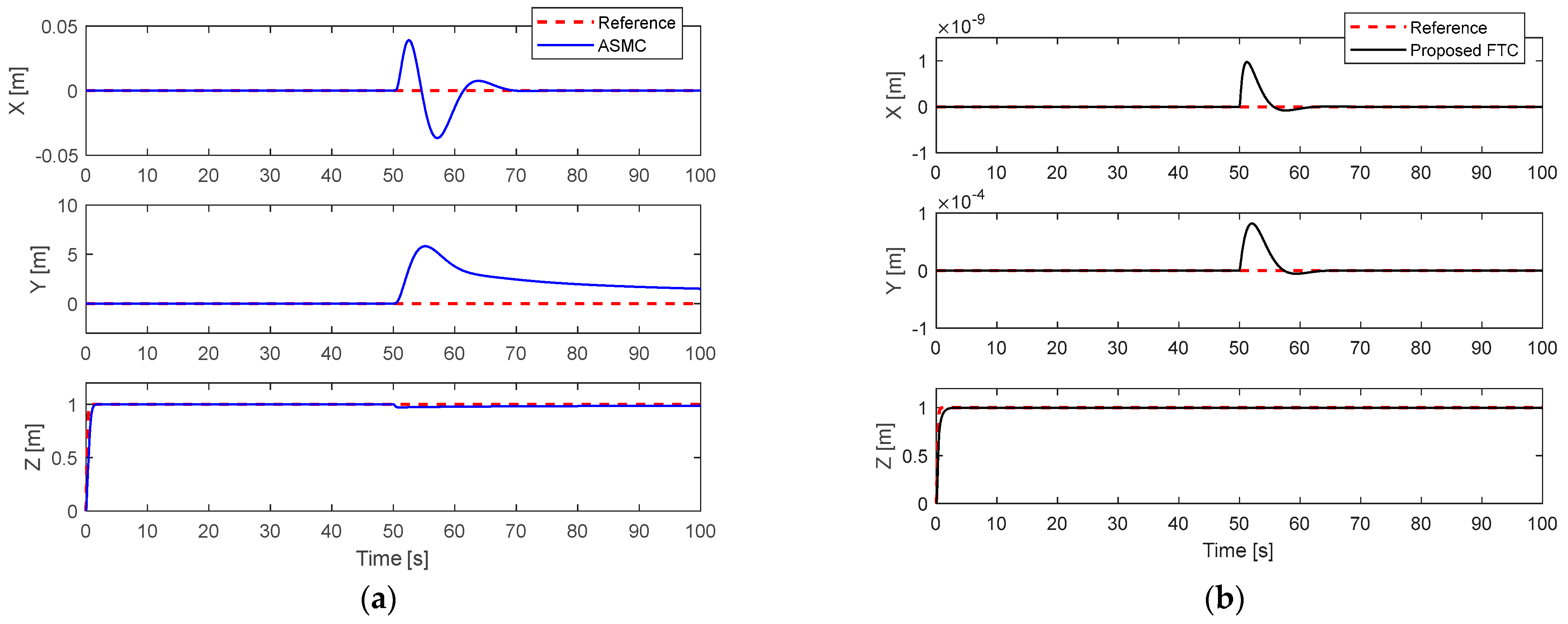
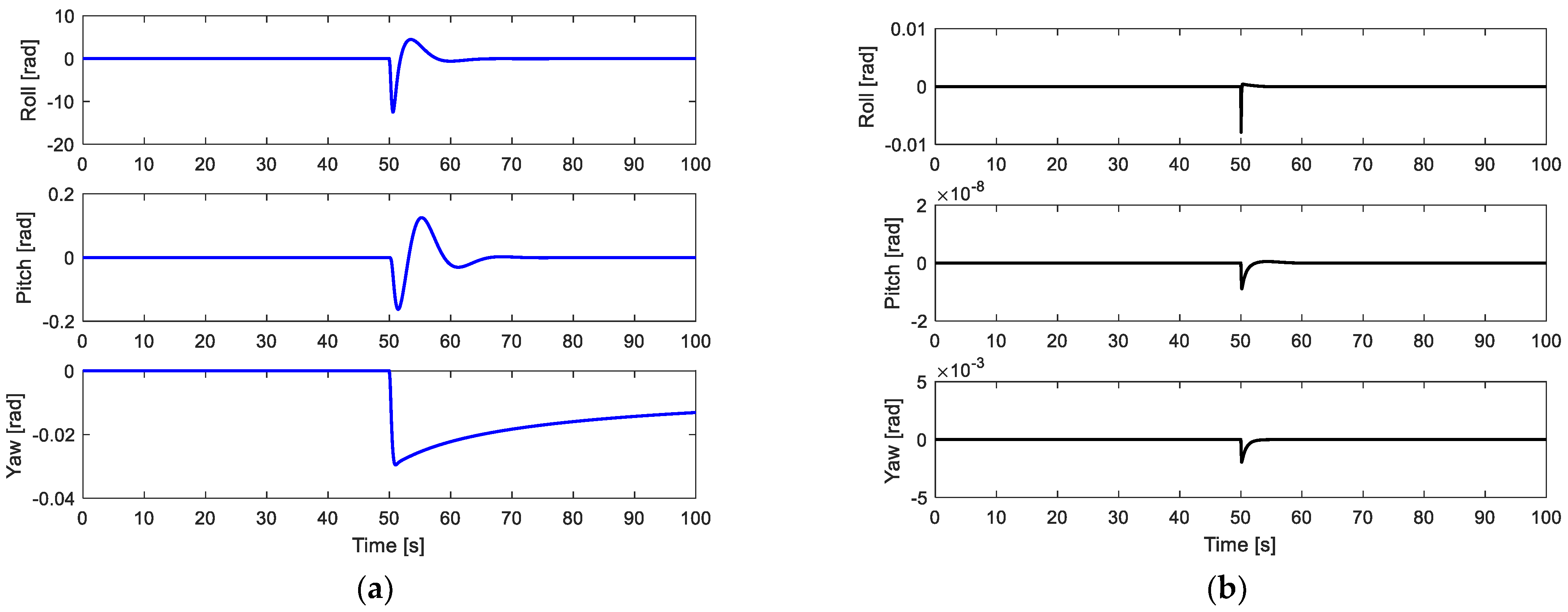
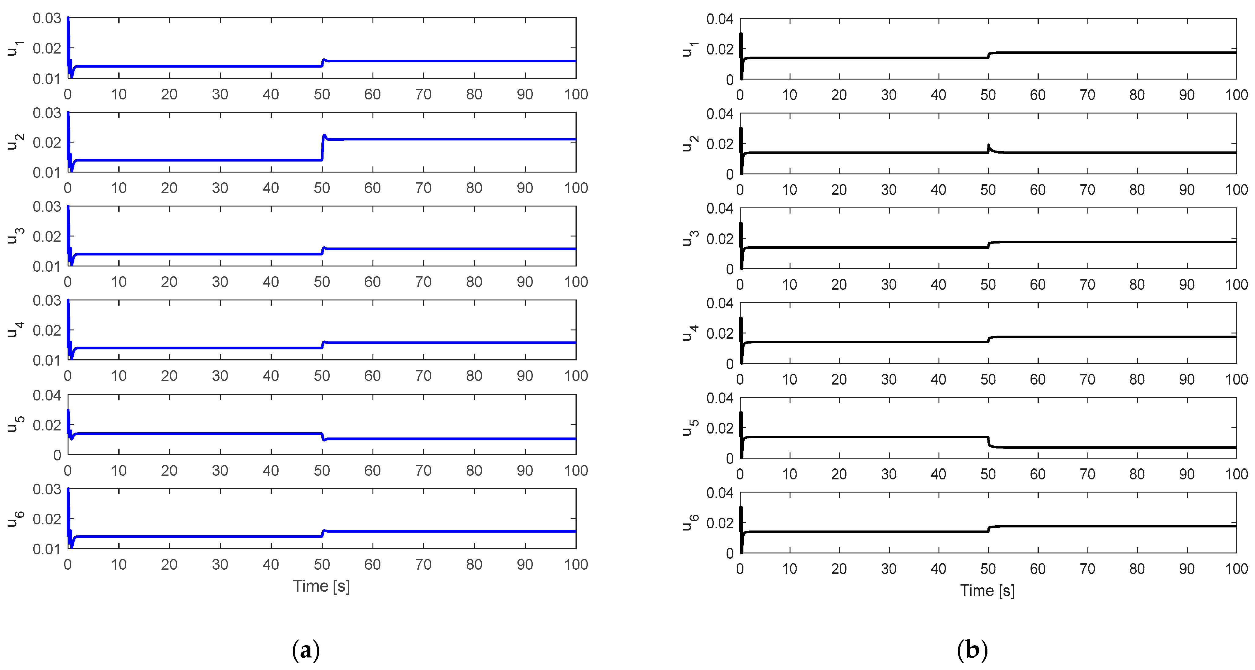
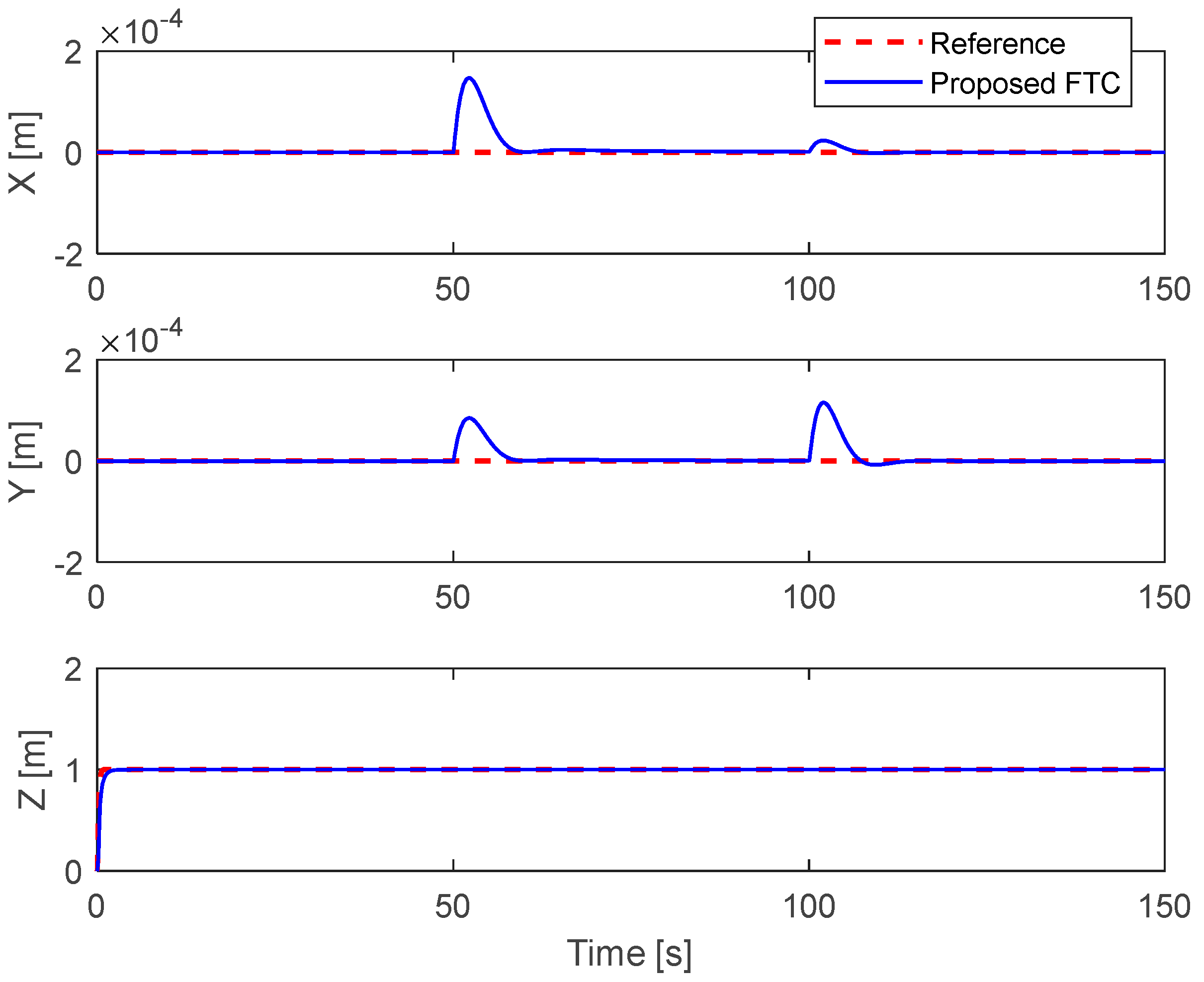
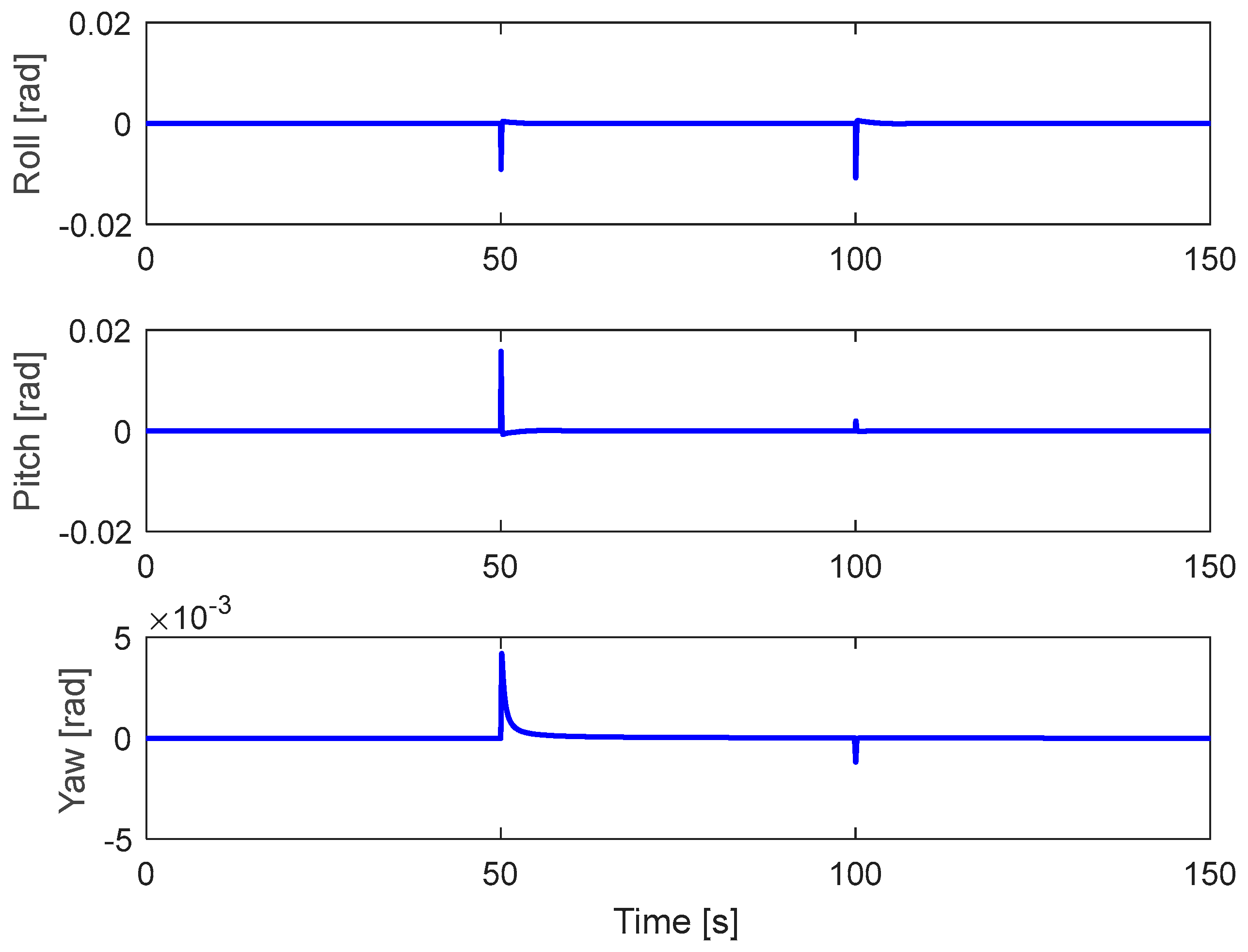
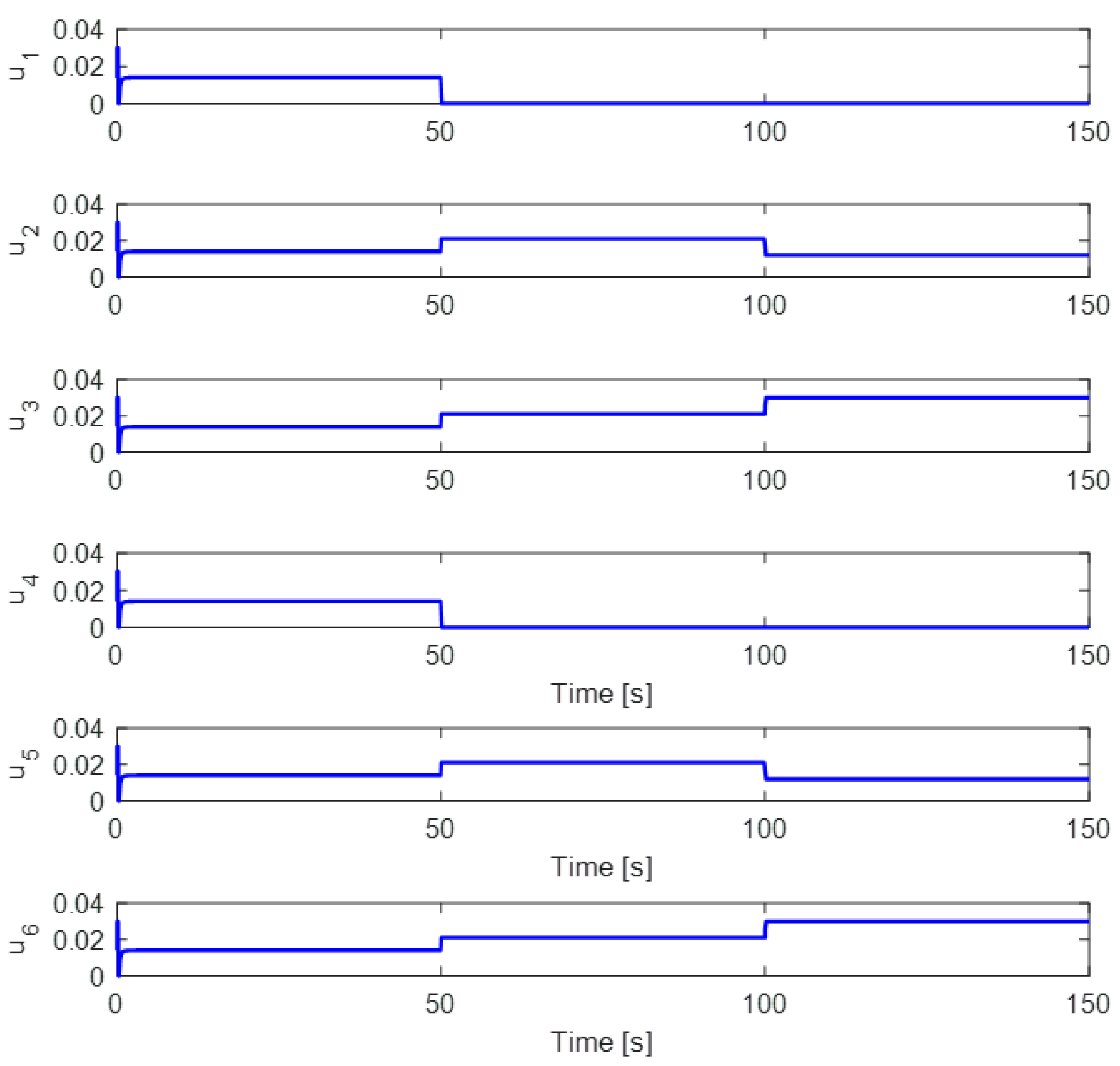
5.2. Complete Fault in Actuator 1 and Partial Fault in Actuator 2

In this scenario, a complete fault and a partial fault were injected into actuator #1 at 50 s and actuator #2, respectively. It is assumed that the hexacopter is made to hover at the desired altitude as $z=1 \mathrm{m}$ and the desired positions $x=0 \mathrm{m}, y=0 \mathrm{m}$. It is shown that the altitude and position performance in Figure 5 can converge quickly to desired values because the proposed FTC of the attitude system can quickly accommodate while making use of the adaptive allocation algorithm. The corresponding attitude performance and motor commands are presented in Figure 6 and Figure 7, respectively. It is clear that to compensate for the complete fault in motor #1, motor #4 needs to decrease its PWM to zero, while the other motors need to increase their PWM at 50 s. After that, to handle the partial fault in actuator #2 at 100 s, motor #3 and motor #6 need to increase their PWM to a value of 0.03, while motor #5 decreases its PWM to a value of 0.015.

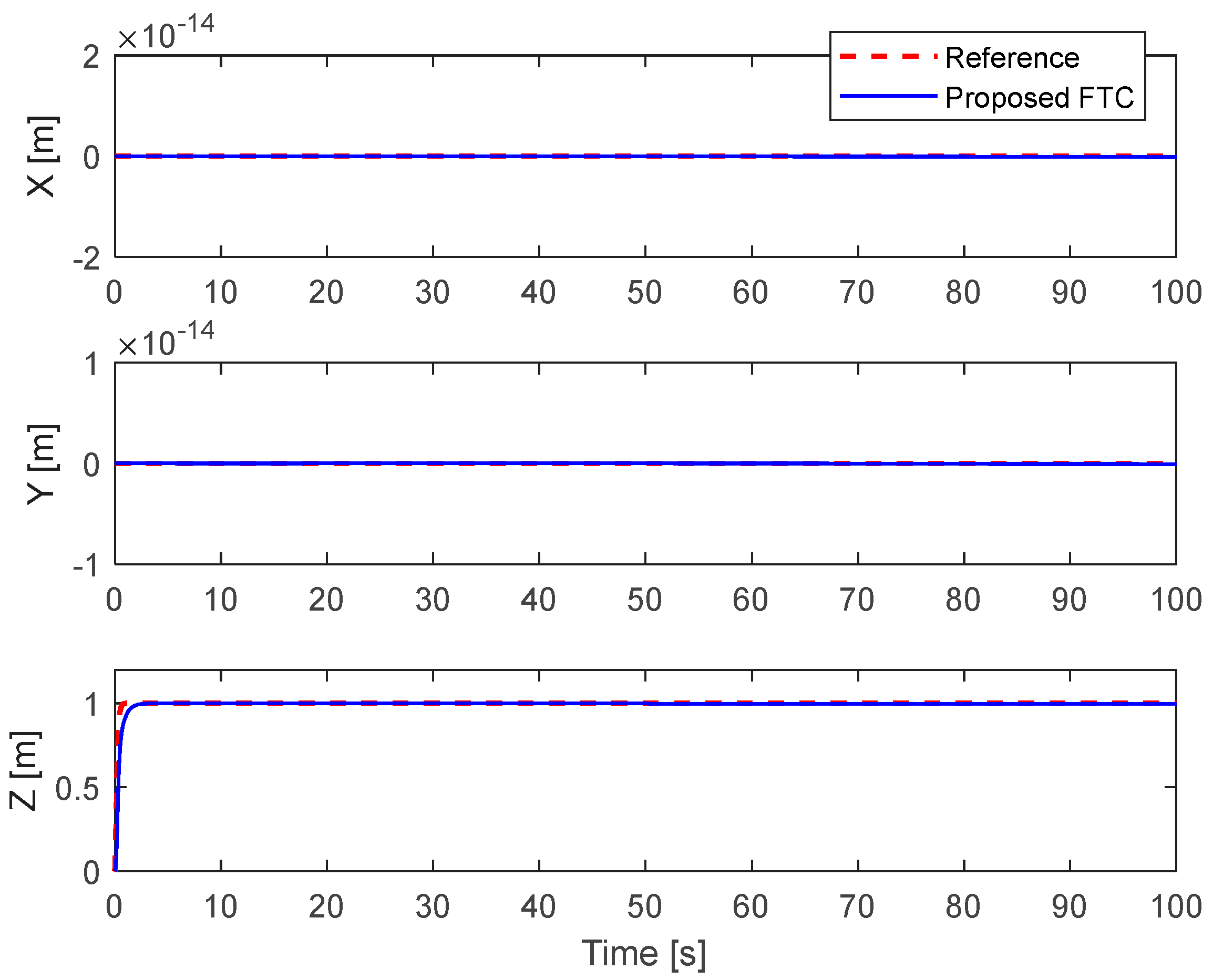
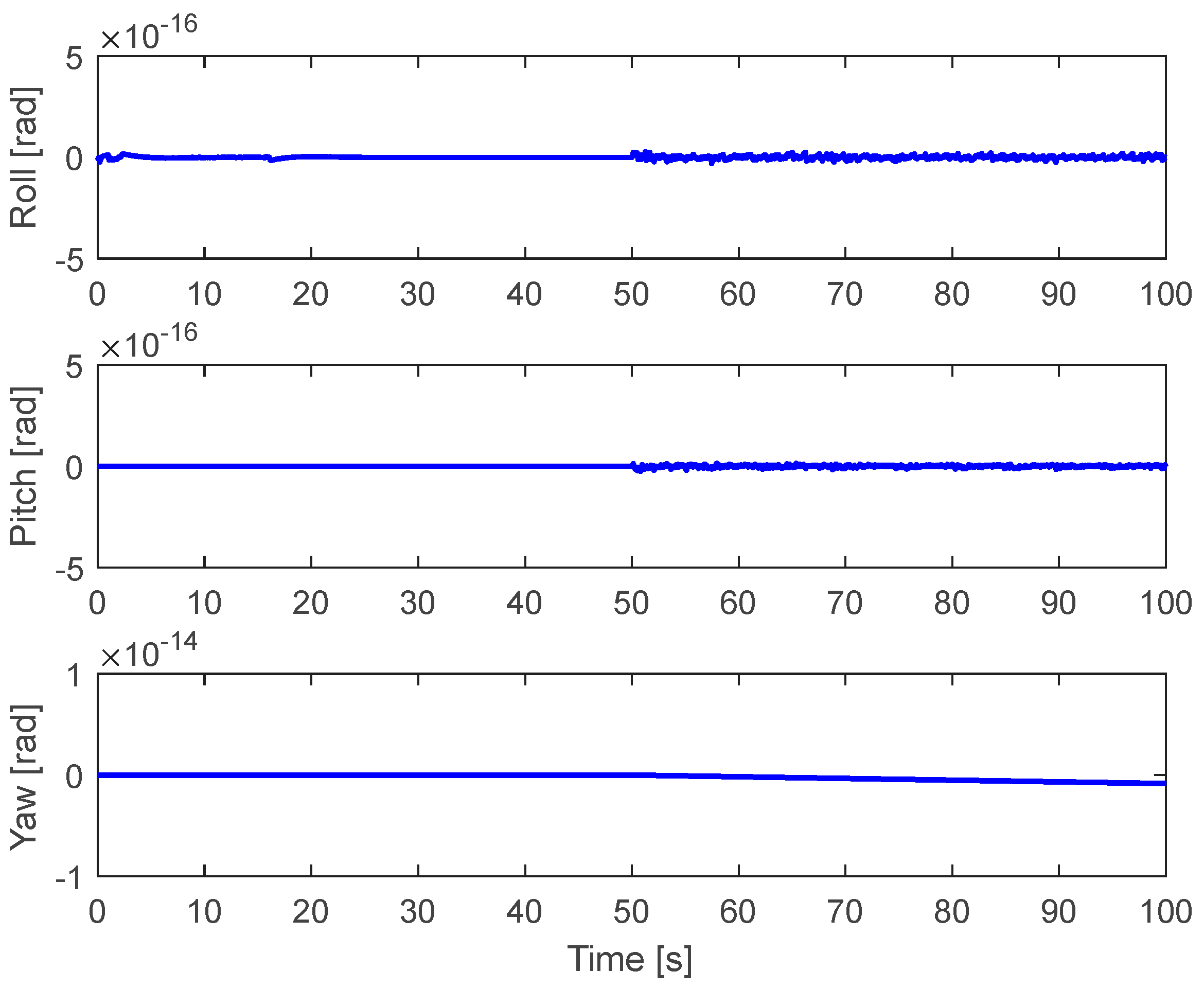
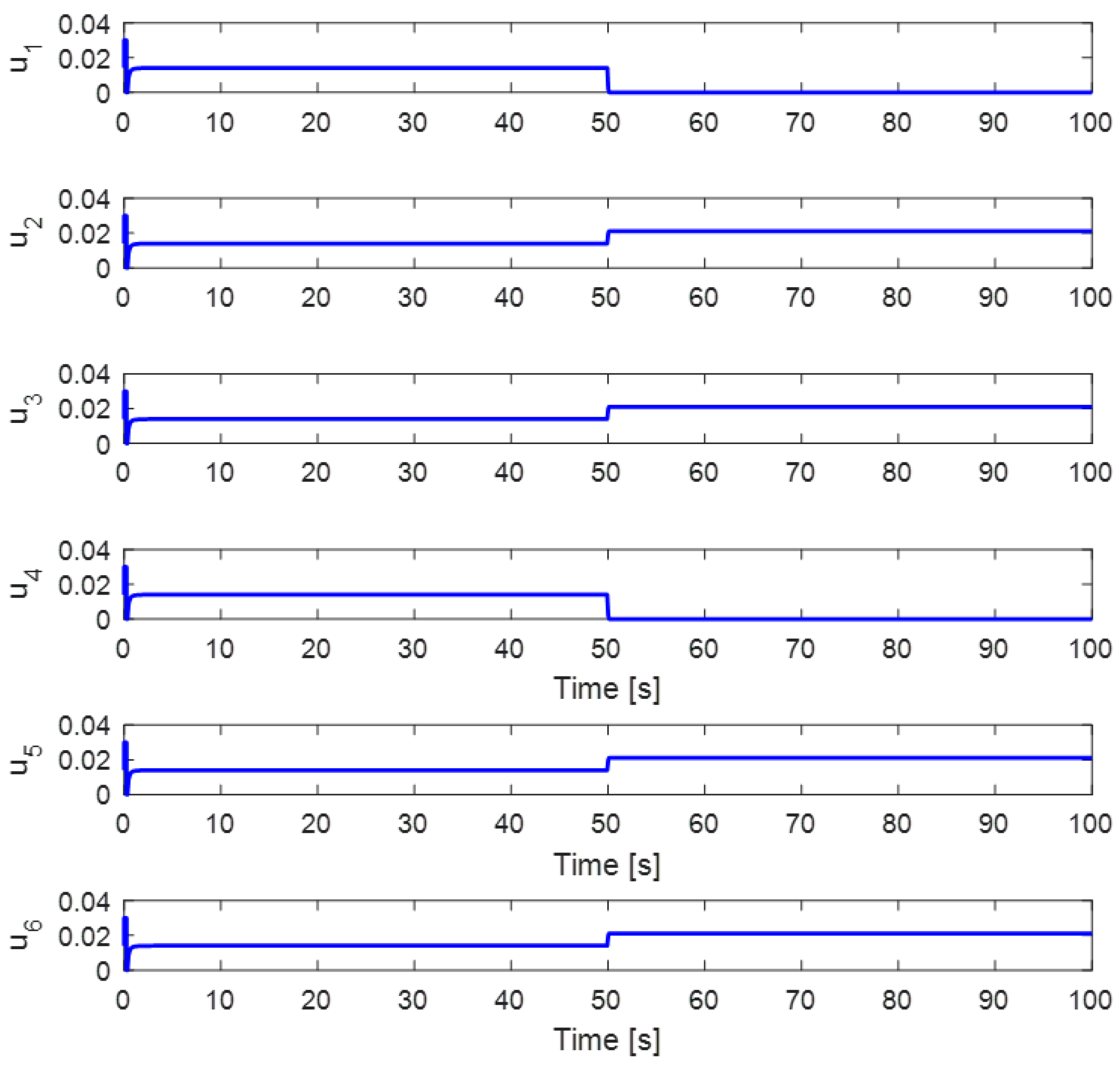
5.3. Simultaneous Fault in Actuator 1 and Actuator 4

In this scenario, the complete fault was injected into actuator #1 and actuator #4 at 50 s simultaneously. The hexacopter is assumed to hover at the desired altitude, as $z=1 \mathrm{m}$ and the desired positions $x=0 \mathrm{m}, y=0 \mathrm{m}$. It is clear that the altitude and position performance in Figure 8 can converge to desired values quickly because the proposed FTC of the attitude system can quickly accommodate while making use of the adaptive allocation algorithm. The corresponding attitude performance and motor commands are presented in Figure 9 and Figure 10, respectively. It is clear that to compensate for the fault, motors #2, #3, #5, and #6 need to increase their PWM.

Remark 1.

Difference to ASMC, the proposed FTC can provide fast compensation through a control allocation algorithm in the presence of model uncertainties. Moreover, the adaptive law in the proposed FTC considered the fault estimation error in the model of a hexacopter due to fault diagnosis problems. Furthermore, the suggested algorithm can handle an unknown complete fault in one motor or complete faults in two opposite motors.

Remark 2.

In example 5.1, the demonstration shows that the proposed control has a good performance compared to ASMC. Therefore, in examples 5.2 and 5.3, only the performance of the proposed control is considered.

Remark 3.

Two complete actuator faults are considered in opposite motors due to controllability. The random complete actuator faults are out of scope of this manuscript, which is a limitation of this paper.

6. Conclusions

In this article, an active FTC method based on an ASMC, and a control allocation scheme are proposed for a hexacopter system. The proposed control method based on control allocation can provide good tracking performance and can handle severe faults through adaptive law, control allocation, and an input saturation algorithm. The stability of the control system is verified using the Lyapunov theory. Simulation results show that the proposed method is better than the adaptive SMC scheme for partial LoCE in a single actuator. Moreover, the results also validate that the proposed approach can handle serve faults in an unknown single complete actuator or even complete faults in two opposite actuators. In future works, the control system will consider sensor faults, wind gust conditions, and noise in the mathematical model. Moreover, the implementation of the proposed method is considered in real-time hardware applications.

References

1. Zhang, Y.M.; Chamseddine, A.; Gordon, B.W.; Su, C.-Y.; Rakheja, S.; Fulford, C.; Apkarian, J.; Gosselin, P. Development of advanced FDD and FTC techniques with application to an unmanned quadrotor helicopter testbed. J. Frankl. Inst. 2013, 350, 2396–2422. [Google Scholar] [CrossRef]
2. Liu, Z.; Yuan, C.; Zhang, Y. Active fault-tolerant control of unmanned quadrotor helicopter using linear parameter varying technique. J. Intell. Robot. Syst. 2017, 88, 415–436. [Google Scholar] [CrossRef]
3. Cen, Z.; Noura, H.; Susilo Younes, Y.A. Robust fault diagnosis for quadrotor UAVs using adaptive Thau observer. J. Intell. Robot. Syst. 2014, 73, 573–588. [Google Scholar] [CrossRef]
4. Cen, Z.; Noura, H. An Adaptive Thau Observer for estimating the time-varying LOE fault of quadrotor actuators. In Proceedings of the 2013 Conference on Control and Fault-Tolerant Systems (SysTol), Nice, France, 9–11 October 2013. [Google Scholar]
5. Lee, C.H.; Park, M.K. Actuator Fault Estimation Method using Hexacopter Symmetry. J. Inst. Control Robot. Syst. 2016, 22, 519–523. [Google Scholar] [CrossRef]
6. Antonio, G.R.; Agus, H.; Poramate, M. Robust actuator fault diagnosis algorithm for autonomous UAVs. IFAC-Pap. 2020, 52, 682–687. [Google Scholar]
7. Alwi, H.; Edwards, C. Fault tolerant control using sliding modes with on-line control allocation. Automatica 2008, 44, 1859–1866. [Google Scholar] [CrossRef] [Green Version]
8. Ban, W.; Youmin, Z. An adaptive fault-tolerant sliding mode control allocation scheme for multirotor hexacopter subject to simultaneous actuator faults. IEEE Trans. Ind. Electron. 2018, 65, 4227–4236. [Google Scholar]
9. Halim, A.; Christopher, E. Sliding mode FTC with on-line control allocation. In Proceedings of the 45th IEEE Conference on Decision & Control, San Diego, CA, USA, 13–15 December 2006. [Google Scholar]
10. Salman, L.; Fuyang, C.; Mirza, T.H.; Lin, Y.; Cun, S. An adaptive integral sliding mode FTC scheme for dissimilar redundant actuation system of civil aircraft. Int. J. Syst. Sci. 2019, 50, 2687–2702. [Google Scholar]
11. Saied, M.; Lussier, B.; Fantoni, I.; Francis, C.; Shraim, H.; Sanahuja, G. Fault diagnosis and fault-tolerant control strategy for rotor failure in an octorotor. In Proceedings of the IEEE International Conference on Robotics and Automation (ICRA), Seattle, WA, USA, 2 July 2015. [Google Scholar]
12. Alwi, H.; Hamayun, M.T.; Edwards, C. An integral sliding mode fault tolerant control scheme for an octorotor using fixed control allocation. In Proceedings of the 13th International Workshop on Variable Structure Systems (VSS), Nantes, France, 29 June–2 July 2014. [Google Scholar]
13. Samir, Z.; Hemza, M.; Abderrahmen, B.; Ali, D. Actuator fault tolerant control using adaptive RBFNN fuzzy sliding mode controller for coaxial octorotor UAV. ISA Trans. 2018, 80, 267–278. [Google Scholar]
14. Hussein, M.; Majd, S.; Hassan, S.; Clovis, F. Fault-tolerant control of an hexacopter unmanned aerial vehicle applying outdoor tests and experiments. IAFC-Pap. 2018, 51, 312–317. [Google Scholar]
15. Nguyen, D.-T.; Saussié, D.; Saydy, L. Fault-Tolerant Control of a Hexacopter UAV based on Self-Scheduled Control Allocation. In Proceedings of the International Conference on Unmanned Aircraft Systems (ICUAS), Dallas, TX, USA, 12–15 June 2018. [Google Scholar]
16. Nguyen, D.-T.; Saussie, D.; Saydy, L. Design and Experimental Validation of Robust Self-Scheduled Fault-Tolerant Control Laws for a Multicopter UAV. IEEE/ASME Trans. Mechatron. 2021, 26, 2548–2557. [Google Scholar] [CrossRef]
17. Nguyen, N.P.; Xuan Mung, N.; Hong, S.K. Actuator Fault Detection and Fault-Tolerant Control for Hexacopter. Sensors 2019, 19, 4721. [Google Scholar] [CrossRef] [Green Version]
18. Sudhir, N.; Swarup, A. On adaptive sliding mode control for improved quadrotor tracking. J. Vib. Control 2017, 24, 3219–3230. [Google Scholar]
19. Asadi, D.; Ahmadi, K.; Nabavi, S.Y. Fault-tolerant trajectory tracking control of a quadcopter in presence of a motor fault. Int. J. Aeronaut. Space Sci. 2022, 23, 129–142. [Google Scholar]
20. Ljaz, S.; Fuyang, C.; Hamayun, M.T. Adaptive non-linear integral sliding mode fault-tolerant control allocation scheme for octorotor UAV system. IET Control Theory Appl. 2020, 14, 3139–3156. [Google Scholar]
Figure 1. Hexacopter in body and inertial frames.
Aerospace 09 00304 g001
Figure 2. Altitude and position performance with 50% LoCE in actuator #2: (a) ASMC; (b) Proposed FTC.
Aerospace 09 00304 g002
Figure 3. Attitude angle performance with 50% LoCE in actuator #2: (a) ASMC; (b) Proposed FTC.
Aerospace 09 00304 g003
Figure 4. Response of motor’s command with 50% LoCE in actuator #2: (a) ASMC; (b) Proposed FTC.
Aerospace 09 00304 g004
Figure 5. Altitude and position performance with complete fault in actuator 1 and partial fault in actuator 2.
Aerospace 09 00304 g005
Figure 6. Attitude angle performance with complete fault in actuator 1 and partial fault in actuator 2.
Aerospace 09 00304 g006
Figure 7. Response of motor’s command with complete fault in actuator 1 and partial fault in actuator 2.
Aerospace 09 00304 g007
Figure 8. Altitude and position performance with simultaneous fault.
Aerospace 09 00304 g008
Figure 9. Attitude angle performance with simultaneous fault.
Aerospace 09 00304 g009
Figure 10. Response of motor’s command with simultaneous fault.
Aerospace 09 00304 g010