Clean Sky 2 Technology Evaluator—Results of the First Air Transport System Level Assessments

Abstract

The authors have adjusted the DLR forecast model to evaluate the environmental benefits in terms of CO₂ and NO_x emissions of Clean Sky 2 technology innovations. The paper briefly describes the model employed: it consists of a passenger/flight volume forecast, a fleet model, and emission modelling. The novelty of the forecast approach compared to previous studies is that it is based on airport pairs instead of larger aggregates like countries or regions. Therefore, a separate breakdown on airports is unnecessary in the case of a more detailed analysis is needed, and it enables us to include airport capacity constraints which affect demand and flight volume, as well as the fleet development at constrained and unconstrained airports. We eventually present the forecast results in terms of passenger and flight volume, fleet development, and CO₂ and NO_x emissions. The results show that emissions can be reduced substantially by the use of Clean Sky 2 technology compared to a reference case which represents the status quo.

1. Introduction

Clean Sky 2 (CS2) was established in order to reduce the environmental impact of air transport by the introduction of new advanced aeronautical technologies. CS2 aims to improve mobility and support a globally competitive European aeronautical industry in Europe by speeding up technological developments. CS2 demonstrates reduction potentials with regard to CO₂ and NO_x emissions of between 20% and 30% compared to state-of-the-art aircraft in 2014.

These general goals have been translated into specific emission reduction objectives for the CS2 concept aircraft models according to their expected entry into service, and ranging from 19-seat commuter to short- and long-range high-capacity commercial aircraft. On the level of the global air transport system, those new concept aircraft have been embedded into two fleet projections up until 2050, and were then compared to a projection without new CS2 aircraft, in order to understand the emission reduction potentials of a future global fleet in 2050, and the long-term aviation footprint. This is the topic of this paper.

A major improvement compared to previous studies, e.g., Clean Sky 1 or manufacturer forecasts like Airbus or Boeing, is the development of a new forecast method. This method is based upon airport pairs instead of more aggregated regions like countries or route groups, as in the case of the approach of the International Civil Aviation Organization (ICAO). In this way, it is possible to include airport capacity constraints, which influence demand volume, the number of flights, and the fleet development at constrained and unconstrained airports [1]. For this paper, all airports with scheduled flight services are included, which is in total about 4000 airports. Furthermore, this approach is more appropriate for airport or aircraft mission-level analysis, as there is no need for a separate breakdown of an aggregate forecast on the study airports. However, airport and aircraft mission-level analysis are not the topic of this paper. We have set out a global forecast until 2035, and two scenarios from 2035 until 2050 on the air transport system level. Nevertheless, the global results are based on the airport pair level, so that it is essentially a bottom-up approach.

In Section 2, we begin with a brief discussion of the methods and models employed for the global impact assessment, which follows in Section 3. Section 4 closes the paper with a discussion of the results, and a series of conclusions.

2. Model Overview

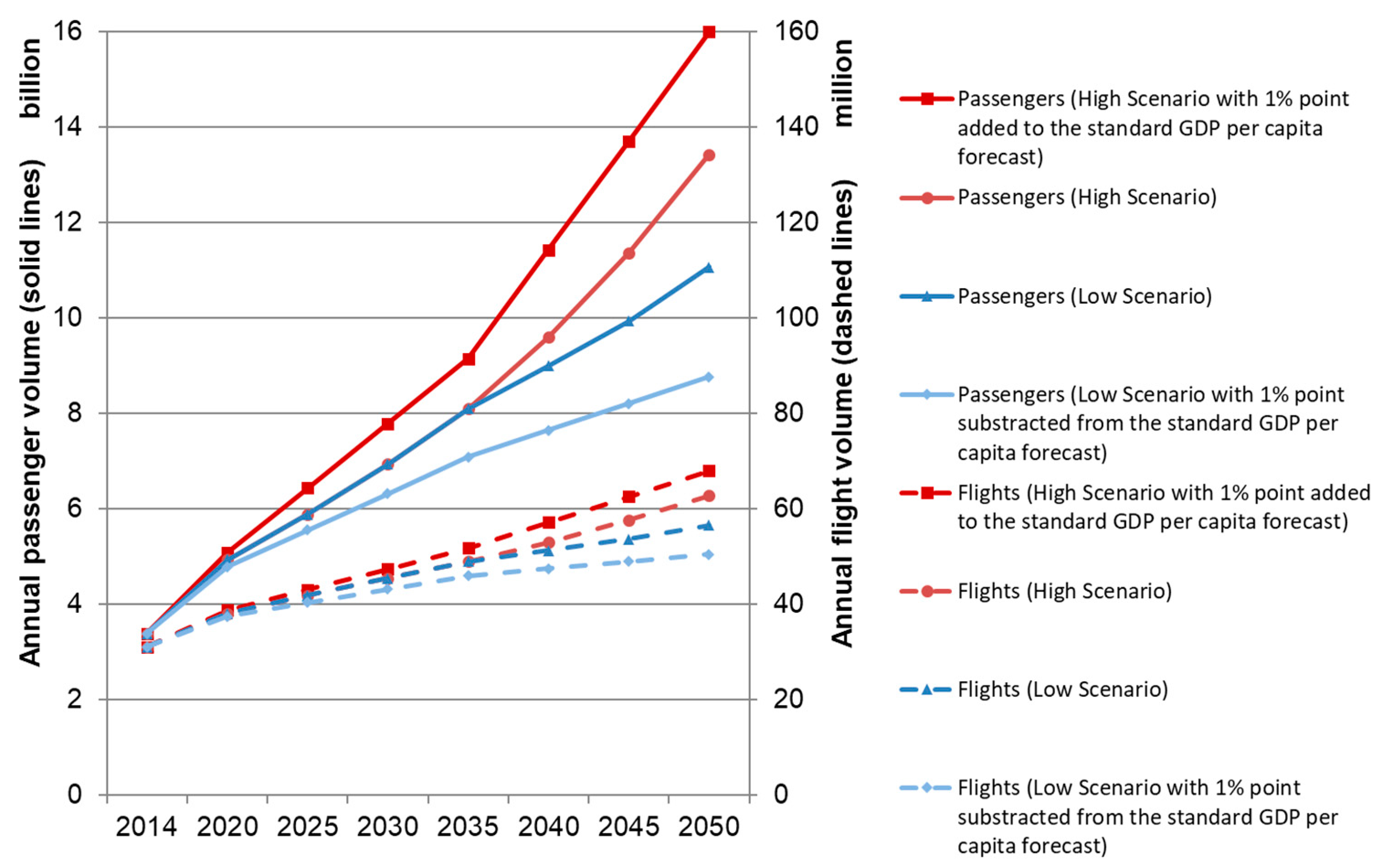
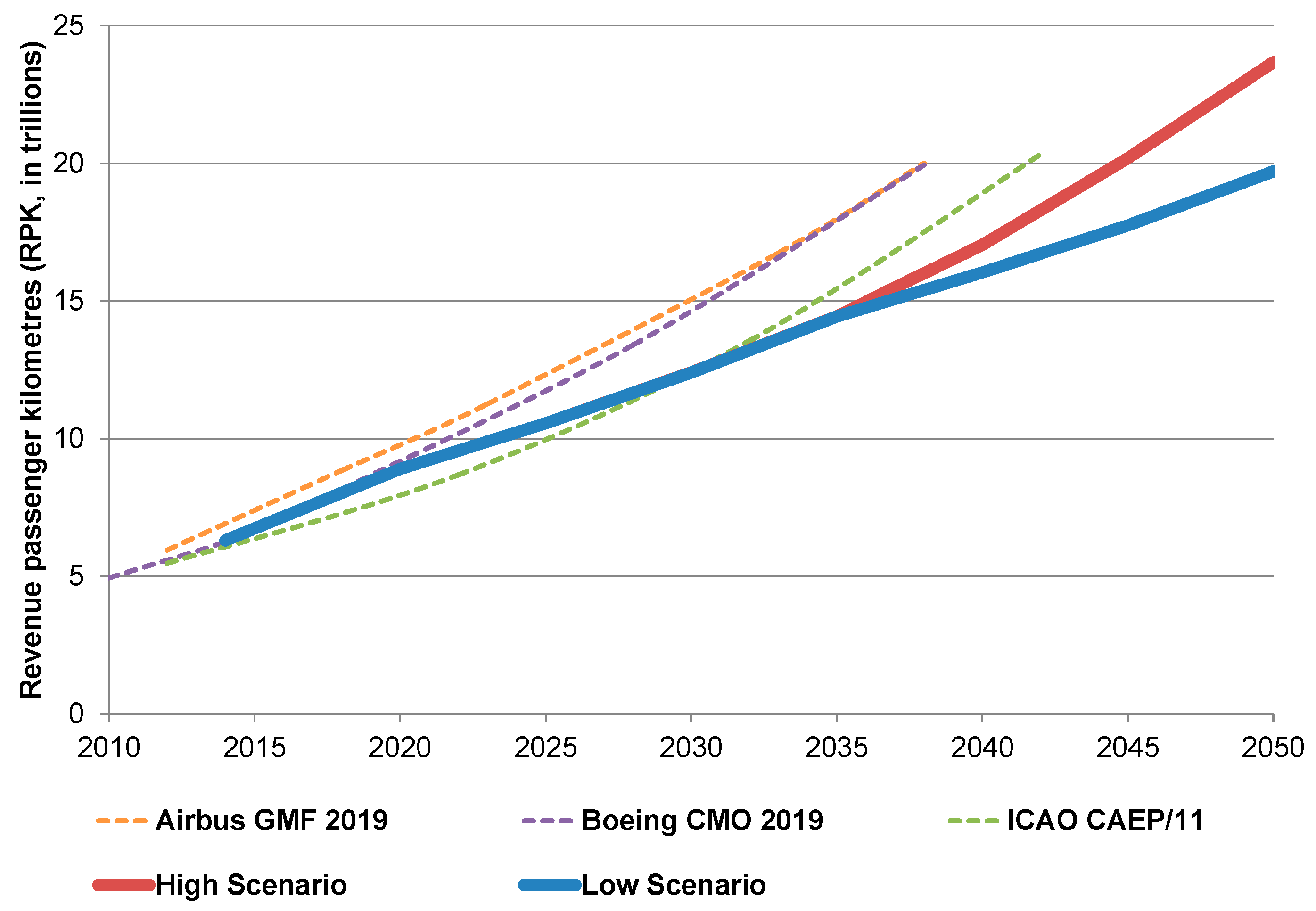
In this chapter we present a brief overview of the approach for the passenger and flight forecast, the fleet model, and the emission modelling. For the time period 2014–2035 we create a single forecast, and from 2035 to 2050 two scenarios are employed. These differ basically in terms of aviation technology and market development. The scenario assumptions have two effects: first, aviation technology development determines the technology of future aircraft. This in turn influences the development of future airfares, which have an effect on passenger demand and, finally, flight volume. For the time period up to 2035 we assume a decline in real airfares, i.e., inflation-adjusted airfares, of 1.5% per year based on data analysis of Sabre AirVision Market Intelligence and inflation data from World Development Indicators [2]. For the time period 2035–2050, we have therefore created two scenarios: in the High Scenario, we assume a more favorable technological and market development, which results in a decline of real airfares of 2.0% per year. On the other hand, in the Low Scenario, we assume a decline of 0.5% per year because of a less favorable development. At this stage, the technological development is rather generic, i.e., it is not related to specific aircraft types. As a result, the two scenarios differ in terms of their demand development, and we simply call them the “High Scenario” and “Low Scenario” in Section 2.1.

In Section 2.2 and Section 2.3, i.e., the fleet and emissions modelling, we use the terms “Reference Scenario” and “CS2 Scenario”. “Reference Scenario” means that only aircraft that were already in service or available for order in 2014 or earlier are employed (“state-of-the-art aircraft” of 2014 or earlier). “CS2 Scenario”, on the other hand, allows the introduction of newer aircraft, especially CS2 concept aircraft. These scenarios are related to specific aircraft types, and they will be explained in more detail later in this paper. “CS2 Scenario” and “Reference Scenario” are therefore specific aircraft technology related scenarios.

These two types of scenarios can be combined, e.g., the CS2 Scenario with the High Scenario or the Reference Scenario with the Low Scenario. In total, we have four combinations, and they are important for the assessment of the emission reduction potential of CS2 concept aircraft. The emission reduction potential of CS2 aircraft is assessed relative to the state-of-the-art aircraft of 2014 in order to identify the contribution of CS2 technology. The results of the Reference Scenario are not reported on their own; they serve as a reference point for the results of the CS2 Scenario.

2.1. Passenger and Flight Forecasts

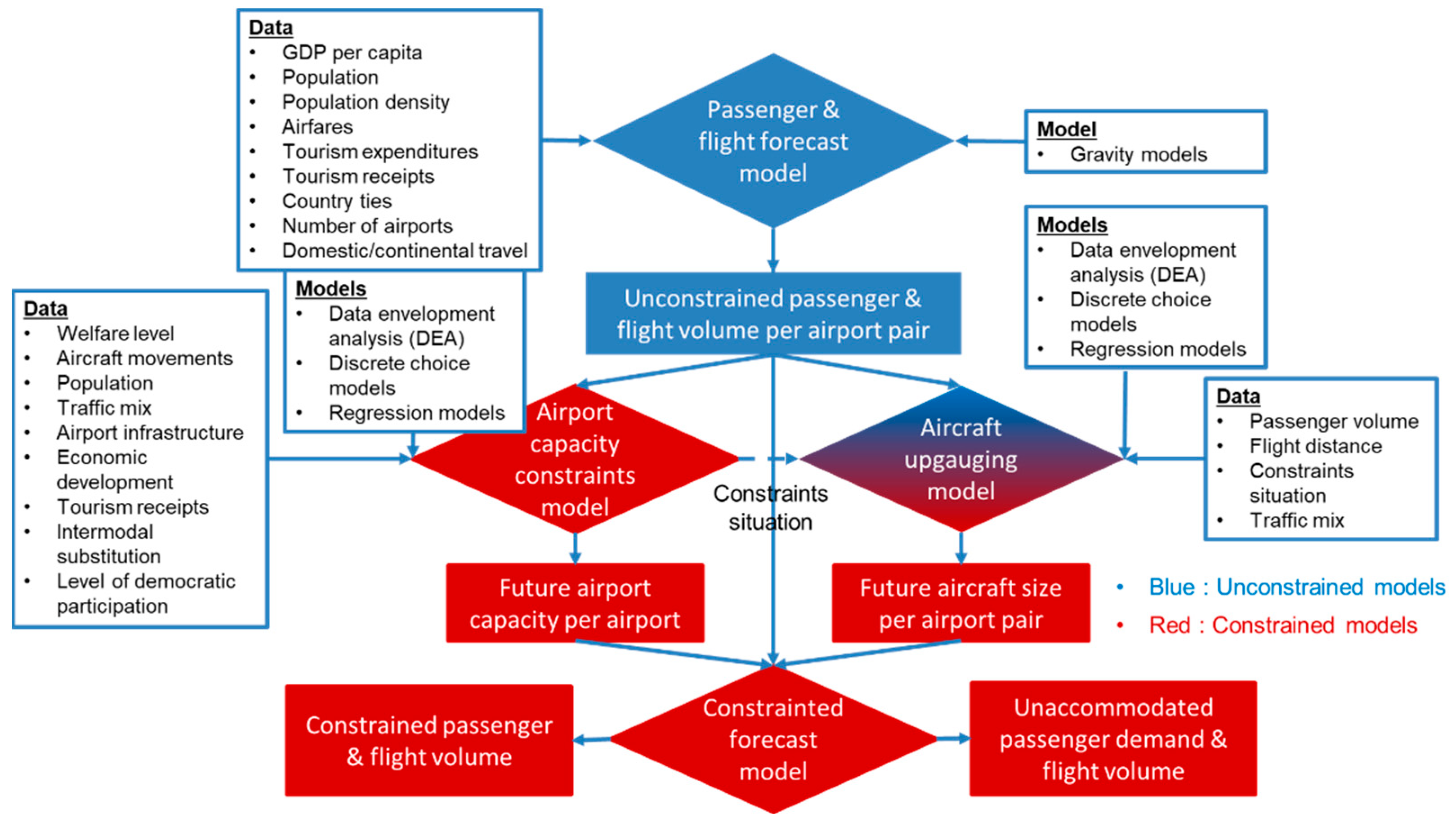
In this section we briefly cover the methodology of the passenger and flight forecasts. For a more detailed description, the reader is referred to [2]. Figure 1 illustrates the model approach:

• In the first step, unconstrained passenger demand and flight volume is forecast for each airport pair.
• In the next step, for each airport pair, the flight volume is compared with the current and expected airport capacity. The forecast passenger and flight volume, as well as the constraint situation at airports, will influence the average future aircraft size, which is forecast for each airport pair.
• In the final step, the expected passenger and flight volume is balanced with airport capacity and aircraft size development to yield the constrained passenger and flight volume. This might result in some unaccommodated passenger demand and flight volume, depending on the severity of airport capacity constraints and the potential of employing larger aircraft.

The relationships between passenger demand, aircraft size and airport capacity are particularly important in a world in which future airport capacity tends to fall short of demand, at least at some airports. Regarding capacity constraints, we mainly focus on the runway system, as this is the most critical element for overall airport capacity in the long term. Especially in Western countries, the enlargement of the runway system requires a plannig approval procedure which involves the public, who are typically opposed to such plans because of environmental concerns, e.g. increased noise levels. On the other hand, other aspects of airport capacity, such as terminal capacity, can be enlarged as part of the airports’ business decisions without the involvement of the public [3]. Employing bigger aircraft is an effective option to mitigate capacity shortages; however, in particular at hub airports, existing network carriers rather tend to increase flight frequency in order to restrict competitors’ access to core markets [4,5]. On the other hand, there are certainly limits to ever increasing aircraft size and transporting more and more passengers per flight. In the case of a high share of feeder traffic, in particular to smaller airports, frequencies are typically higher [6].

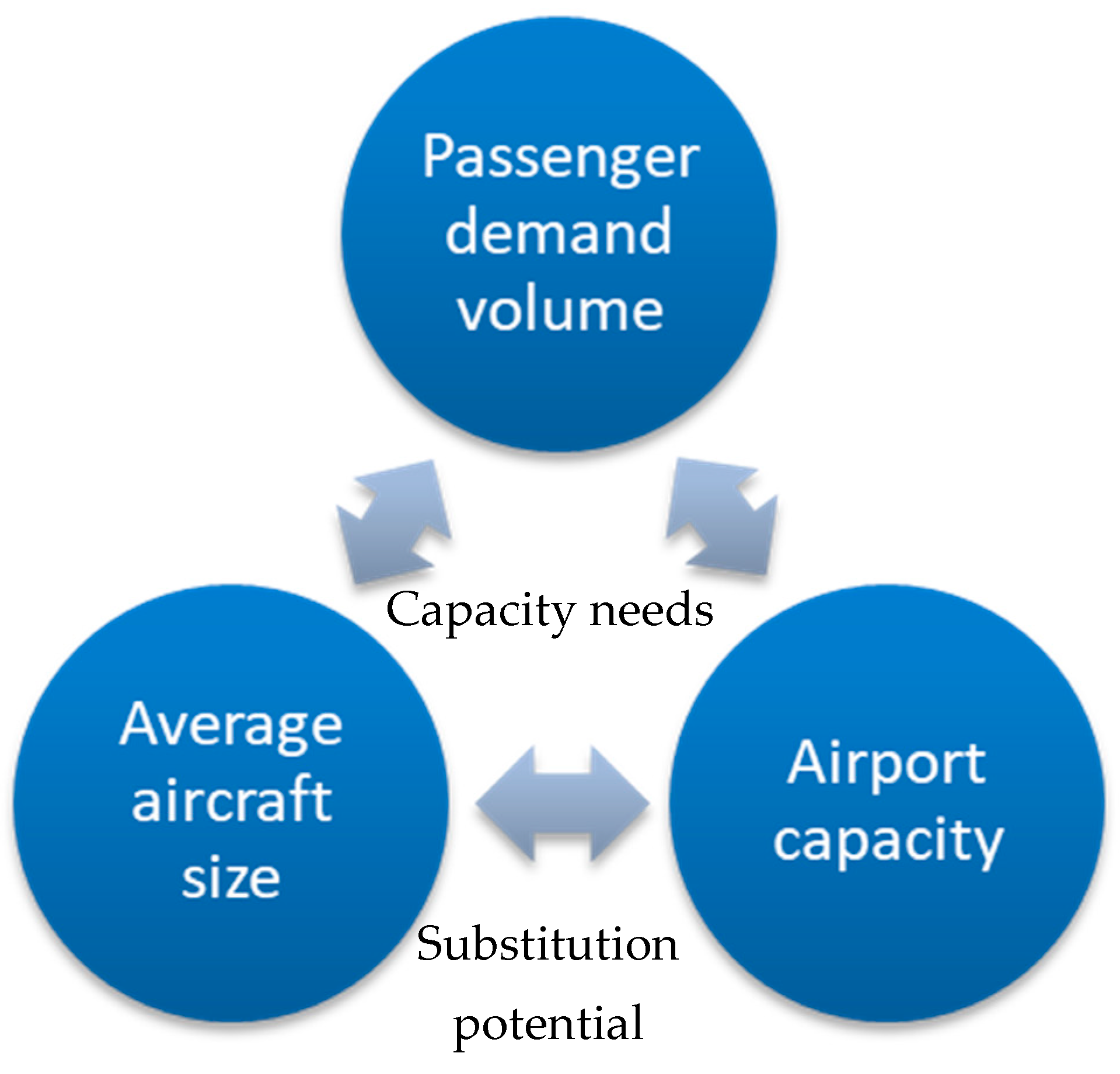
Figure 2 displays the relationships between the passenger demand (annual passenger volume), airport capacity (annual flight volume) and average aircraft size (passengers per aircraft) on a very general level: in order to accommodate the forecast passenger demand, airport capacity in terms of flight movements is required, in combination with a pre-determined average aircraft size (which is endogenous to the model). Both the average aircraft size and the airport capacity limit the maximum number of passengers that can be handled. Aircraft size and airport capacity can be substituted for each other to some degree: if the airport capacity is insufficient to serve a given passenger demand, increasing aircraft size can compensate for a lack of airport capacity to serve that demand. A lack in terms of aircraft size can be compensated for by more airport capacity, so that more flights—but with, on average, fewer passengers per flight—can be handled. However, as already explained earlier, typically airport capacity is the bottleneck.

The model accounts for these interrelations between passenger demand, airport capacity and aircraft size by adjusting all three elements in a constrained forecast. In contrast, an unconstrained forecast always assumes the best case regarding the future development of airport capacity. Moreover, unconstrained forecasts underestimate the long-term increase of average aircraft size, i.e., the average number of passengers transported per flight, as a measure to compensate for the shortfall in airport capacity.

Shifting traffic to neighbour airports can be another option to mitigate capacity constraints. Gelhausen [8] shows that, from a passenger’s perspective, such a shift can theoretically happen in a decentralised or multi-airport environment. Gudmundsson et al. [9] identify spillover effects between London Heathrow and Gatwick, and to a lesser degree between Heathrow and Stansted (and even to the more remote airports Birmingham and Manchester). However, if they control for low-cost carrier effects, they only find spillover effects between Gatwick and London City airports in European traffic. Redondi and Gudmundsson [10] find significant spillover effects of constraints at London Heathrow and Frankfurt airports in stop-over traffic in European and Gulf hub airports. Dennis [11], on the other hand, argues that shifting flights to less-congested airports is simply not compatible with the demands of passengers and hub airlines. Currently, this is a very difficult topic to implement in a sound way, especially on a global level, and therefore certainly needs more research. The main questions are: What share of excess traffic is shifted to which airports? Is excess traffic only partially or fully shifted to neighbour airports? Currently, it seems that the potential of shifting traffic to neighbour airports is rather limited, and the model currently does not contain a (full) shift of excess traffic to airports in the vicinity.

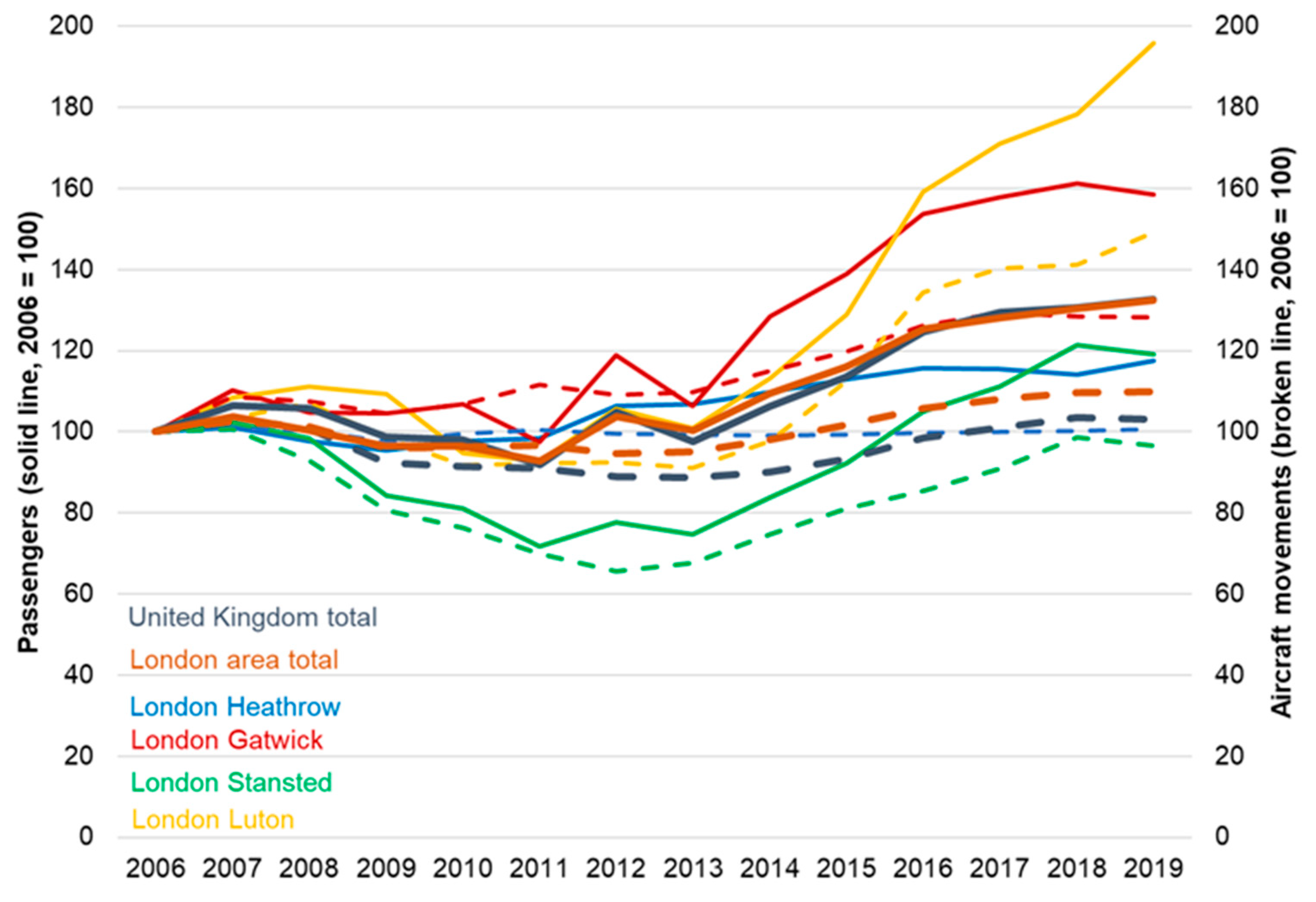
In order to illustrate this point in more detail, we have chosen the London area, which serves as a prime example of a region with a heavily constrained hub airport (London Heathrow), surrounded by another major airport (Gatwick) and two secondary airports (Stansted and Luton) with ample capacity reserves. We have excluded London City airport from the analysis, as it has only limited means of absorbing excess traffic from London Heathrow because of its restricted location in the London Royal Docks, and it can be served only by small aircraft.

London Heathrow has already been constrained for about 20 years, and there has been a long debate about its expansion [12]. Figure 3 illustrates the development of passenger volume and aircraft movements at these four airports, as well as for the London area and the UK between 2006 and 2019 relative to the volumes of 2006. If we look at the UK or the London area as a whole, aircraft movements have remained more or less constant in the UK, and increased by 10% in the London area. Passenger volumes, on the other hand, increased by 33% between 2006 and 2019, both in the UK and in the London area. Of the smaller airports, only Luton increased its flight volume significantly, by around 50%, and in the case of Stansted there was even a decline in the number of flights. The flight volume remained constant at Heathrow, and increased at Gatwick by about 30% since 2006; however, this was much less than passenger volume, which increased by almost 60% since 2006. As we can see, a large share of the passenger volume growth has been accommodated by increasing the number of passengers per flight.

Our forecast model consists of four distinct sub-modules:

• Air passenger demand, which is origin–destination (OD) passenger flows, and the total passenger flows including transfer passengers, between countries as well as airports.
• Airport capacity and capacity utilisation.
• Airport capacity enlargements and limits.
• Average aircraft size: the average number of passengers per flight.

2.1.1. Air Passenger Demand

Well-known long-term forecasts of global air traffic are typically conducted by aircraft manufacturers such as Airbus [13], Boeing [14], and supranational organisations like the ICAO [15]. In the academic literature, the gravity model is still the workhorse of spatial demand modelling. One of the first gravity models employed in air transport research was developed by Harvey [16] to analyse airline traffic patterns in the USA. Grosche et al. [17] employed two gravity models to estimate the air passenger volume of city pairs without any air service. Tusi and Fung [18] analysed passenger flows at Hong Kong International Airport, and focused on a single airport. Matsumoto [19] and Shen [20] based their gravity models on network analysis: Matsumoto’s model was used to estimate passenger and cargo flows between large cities such as Tokyo, London, Paris and New York, while Shen’s was used to analyse inter-city airline passenger flows in a 25-node US network. Bhadra and Kee [21] employed a gravity model to analyse demand characteristics, such as the fare and income elasticities of the US origin–destination market over time. Endo [22] developed a gravity model to analyse the impact of a bilateral aviation policy between the USA and Japan on passenger air transport, while Hazledine [23] used a gravity model to analyse border effects in international air travel. The gravity model has also been applied in air freight modelling: Alexander and Merkert [24] developed a gravity model to evaluate the air freight market in Australia. Later, Alexander and Merkert [25] analysed US international air freight markets in light of the 2008/09 financial crisis. Baier et al. [26] developed a gravity model with airport fixed effects to model global air freight between airports.

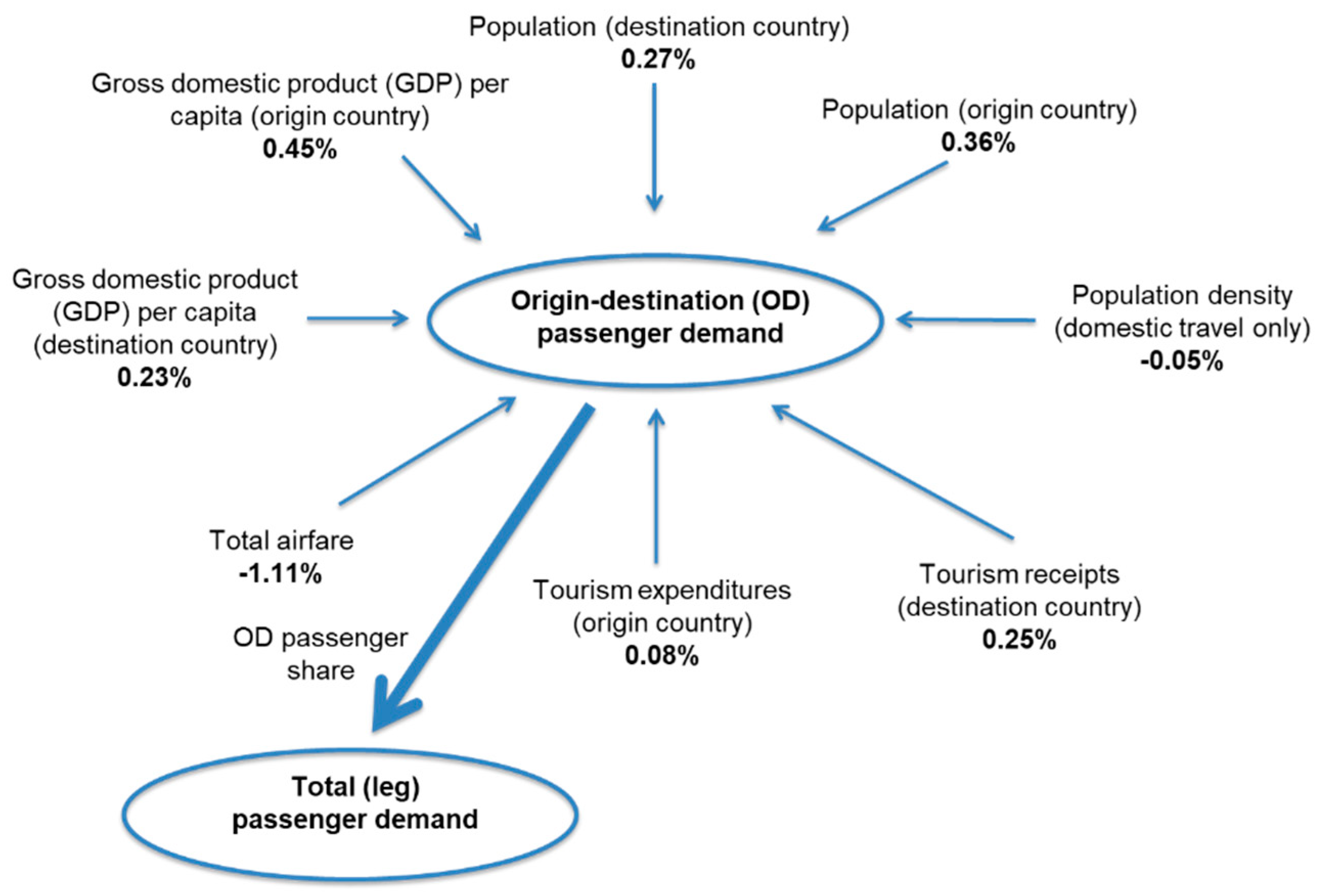
The air passenger demand model that is employed in this paper is also based on the gravity model. Whilst variables such as distance, population and gross domestic product (GDP) are common in gravity models, we expect further insights from the inclusion of an airfare variable. The model was estimated on Sabre AirVison Market Intelligence data [27], which includes information on actual airfares paid by air passengers. From the model estimation, we found airfare elasticity to be −1.11%, i.e., if airfare decreases by 1% then OD air travel demand rises by 1.11%; it is thus slightly elastic. For better discrimination between different types of origin and destination, we included variables such as tourism receipts and expenditure, and population density. Tourism receipts and expenditures are measures for the tourism affinity of the destination and origin country. They both have a positive influence on OD demand; however, tourism receipts have a higher impact. Population density, which is only relevant for domestic air travel, is a measure for mode substitutability: the higher the population density is, the better developed and more relevant the road and rail network for domestic travel is typically in terms of travel time. Take for example the US, which has a population density of about 36 people per km², and Germany, which has a population density of about 232 people per km². The rail and road networks are relatively better developed in Germany compared to the US. For example, travelling from Hamburg to Munich by car or train is more relevant than for the journey from New York City to Los Angeles: for the trip from Hamburg to Munich, you need about one and a half hours by plane (excluding access and egress times), around eight hours by car, and five and a half hours by train (again, excluding access and egress times). For the trip from New York City to Los Angeles, you need nearly six hours by plane, 41 h by car, and more than two and a half days by train. Of course, the distance is much longer between New York City and Los Angeles than between Hamburg and Munich (about 600 vs. 4000 km great circle distance), but cars and trains are relatively faster for Hamburg–Munich, and the planes are relatively faster in the case of New York City–Los Angeles, even though the relative advantage is substantially larger for planes than for cars and trains. As a result, population density has a slightly negative impact on OD air travel demand. The model contains further variables of lesser importance, like distance and country ties [2].

For model estimation, we employed a Poisson pseudo-maximum likelihood (PPML) estimator to produce better and more reliable forecasts [28]. As a result, a series of relevant demand elasticities (see Figure 4) were estimated, e.g., if the GDP per capita increases in the origin country by 1%, then OD passenger demand rises by 0.45%, and if GDP per capita rises in the destination region by 1%, the OD demand grows by 0.23%.

Due to a lack of consistent global data, there is no differentiation between business and leisure passengers. There are only individual surveys covering particular markets like Germany and the UK. We do have information about the share of ticket categories for each airport pair, e.g., from Sabre AirVision Market Intelligence, but it is not possible to infer the share of business travellers from the share of business tickets, as many business travellers choose the economy class. For example, in Germany, 69% of domestic air travel in 2003 was business, and 28% of all European and intercontinental trips from Germany were for business purposes [29]. However, based on the analyses of such surveys, Mason [30] estimates the share of business passengers to be about 30%, but it is not possible to break down this number to the country or airport pair level, which is needed for consistent model estimation.

2.1.2. Airport Capacity and Capacity Utilisation

The global airport capacity model is based upon data envelopment analysis (DEA) and regression analysis. DEA is a non-parametric empirical method used in operations research to estimate production frontiers employing linear programming techniques. DEA is a standard tool for efficiency analyses, and for the benchmarking of so-called decision-making units (DMUs) [31,32]. DEA allows us to compare DMUs which differ in their input and output structures. Examples of such DMUs include hospitals, energy production, or the cost-/profit centers of large organisations and, in our case, airports. The model analyses airport capacity utilisation with one main question in mind: Which airport achieves what output given a particular input structure? In our model approach, this enables us to compute the current and future annual service volumes of airports worldwide. The model allows the forecasting of the 5% peak hour volume and the average hourly volume of an airport in a situation of the highest possible capacity utilisation.

The model produces robust results using input information which is generally available, e.g., the runway system, as this typically limits overall airport capacity in the long term. For our generic airport capacity model, we aimed for an as-high-as-possible degree of accuracy on average on the global level, but we do not pretend that it is as accurate as detailed airport capacity analyses for specific airports. Nevertheless, the results are surprisingly accurate on the airport level. For a comparison with the US and some European and Asian airports, the reader is referred to [2].

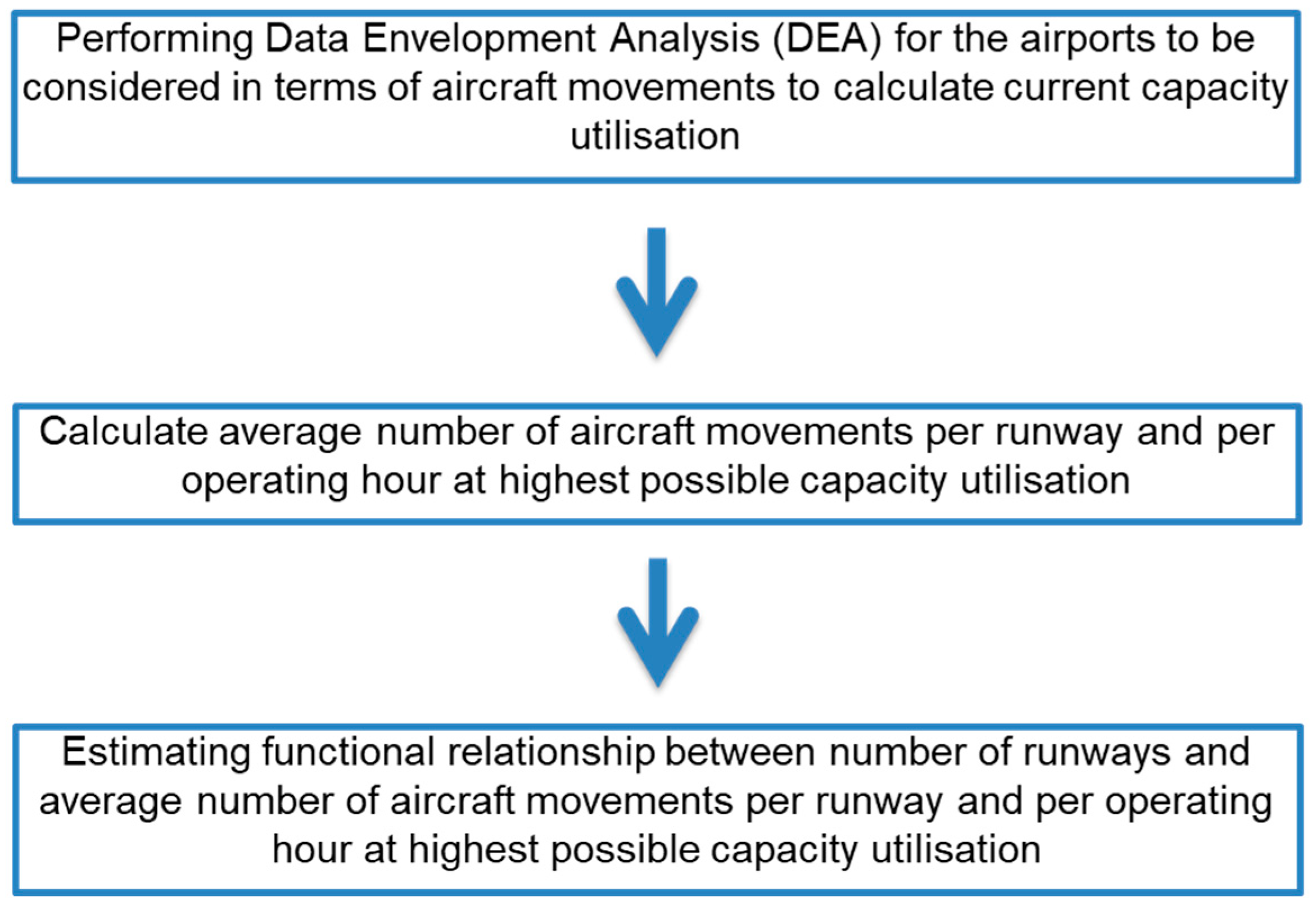
Figure 5 provides an overview of the generic airport capacity model process:

• The first step is the use of the aforementioned DEA to estimate the current airport capacity for airports of interest.
• In a second step, the average number of aircraft movements per runway and per operating hour at the highest possible level of capacity utilisation for each airport is calculated.
• The last step is to perform a regression analysis based on the results of the DEA.

2.1.3. Airport Capacity Enlargements and Limits

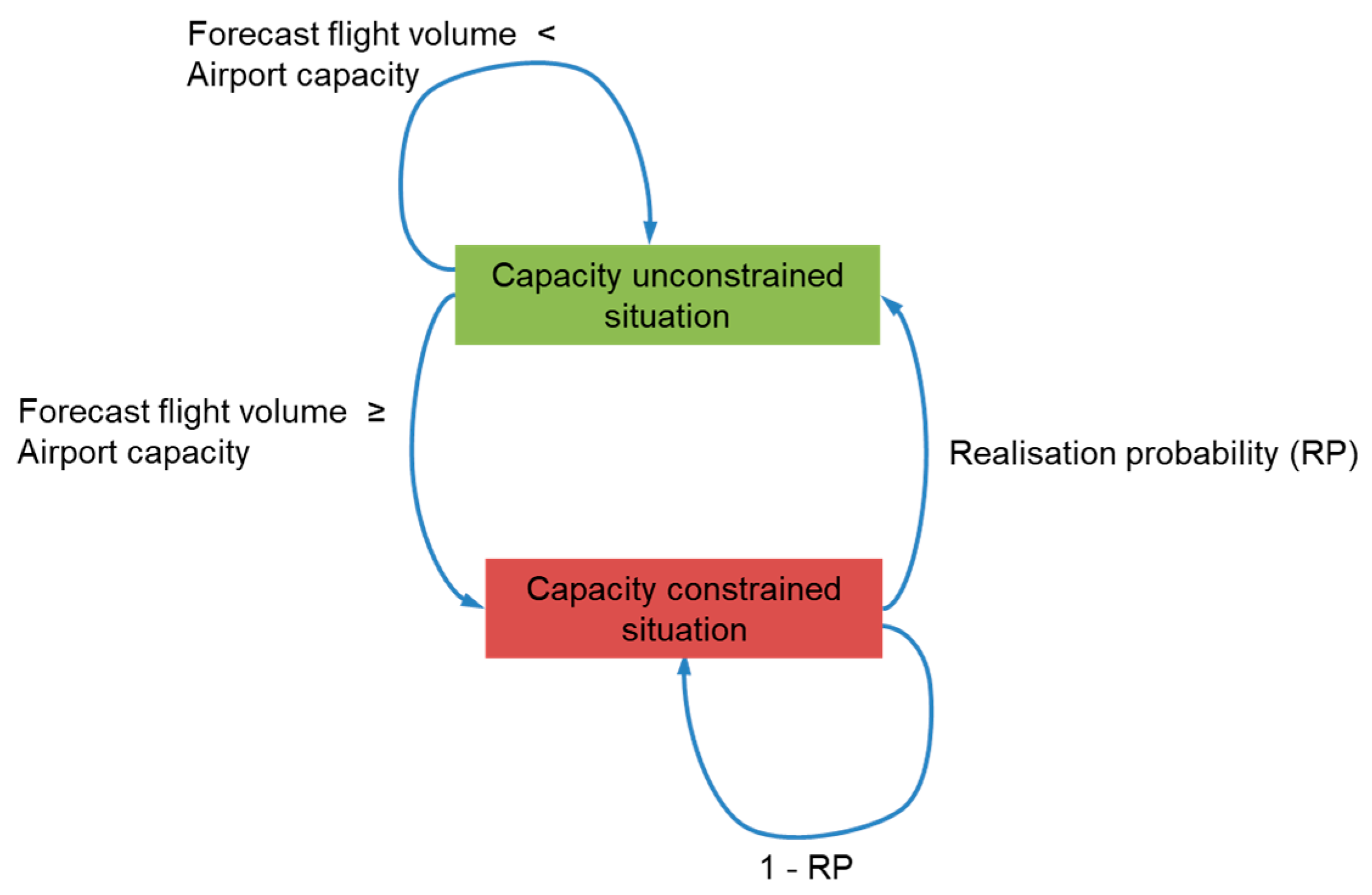
With the model of forecasting the realisation probabilities of airport capacity enlargements and limits, we have introduced an approach which incorporates the enlargement of limited airport capacity in air transport forecasts. If the forecast number of flights exceeds the current airport capacity, the model analyses whether adding new runways is possible, and if this is the case, how long this process is expected to take. This analysis is conducted for each airport and each new runway at that airport. The model is based on the idea that there is a particular degree of opposition to airport expansion from the population living in proximity to the airport. This depends on factors such as noise annoyance, pollution, welfare level, economic opportunities, participation level, and intermodal substitution. The degree of opposition may range from almost none to such an intense opposition that airport expansion is virtually impossible. As a result, the model enables us to estimate the probability of the realisation of a new runway, which can be transformed into an expected value in terms of delay. The approach used is a probabilistic one based on Markov chains [33] and discrete choice theory [34]. The Markov chain comprises of two situations that an airport can face (see Figure 6):

• Situation one: forecast demand < airport capacity.
• Situation two: forecast demand ≥ airport capacity.

Entry into situation two is triggered by the underlying demand forecast and the current capacity of the airport. If the airport is in situation two, the realisation probability (RP) of an additional runway corresponds to the transition probability from situation two to situation one. Eventually, based on the probability of delay, we can calculate the expected delay of runway capacity expansion, as it is the inverse of the transition probability minus one, because 100% RP is defined as no delay in the model with, theoretically, the new runway being instantly available. The realisation probability of runway expansion is modelled by means of a binary logit model [35]. Of course, it is difficult to define an exact threshold above which an airport is capacity constrained. It is a more or less a smooth transition from an unconstrained into a constrained situation, where participation in the general traffic growth becomes increasingly difficult. We can assume that an (artificial) threshold that separates constrained from unconstrained airports lies in a range of 75% capacity utilisation [36]. In the light of this definition, there were ten of about 4000 airports which were capacity constrained in 2008, such as Shanghai (SHA), London Heathrow (LHR) and New York LaGuardia (LGA) [36]. Until 2050, we expect the number of airports to increase to 24 in the Low Scenario and 36 in the High Scenario. These calculations already include new runways that have been built since 2008 (e.g., the fourth runway at Frankfurt airport in 2011) or are expected to be realised by 2050 according to the model’s forecast, shifting traffic to off-peak hours and employing larger aircraft.

2.1.4. Average Aircraft Size: Average Number of Passengers per Flight

The fourth sub-model is on the forecast of passengers per flight by airport pair. As in the case of airport capacities, the approach is highly problem-specific, and cannot be a substitute for a detailed flight route analysis in terms of aircraft fleet characteristics and their future development. The method is very similar to the modelling of airport capacities. The basic analysis is a DEA, which is further refined by regression analyses to generalise the results, so that they can be used for forecasting purposes.

The average number of passengers per flight between an airport pair is determined by the passenger volume of that airport pair, the flight distance, and the constraint situation at the origin and destination airport [2]. The results serve as an input for the more elaborate fleet modelling presented in the next section.

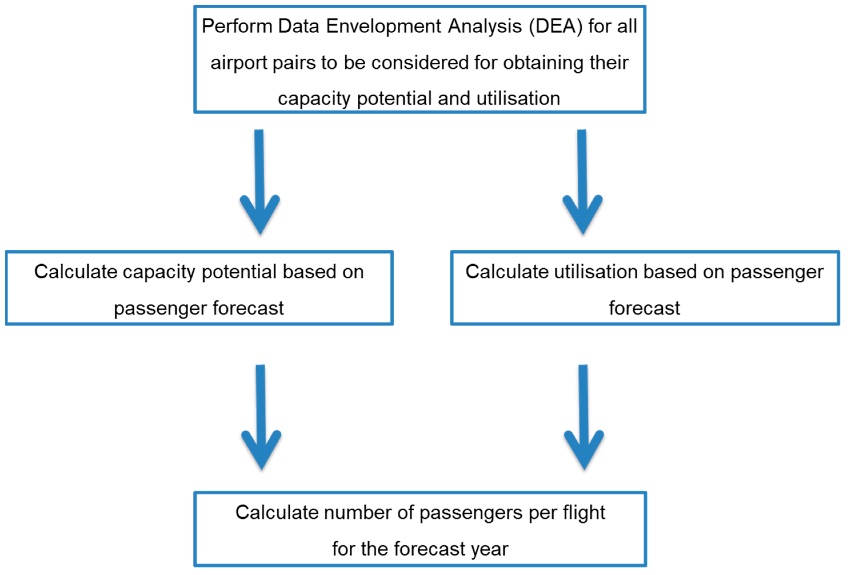
Figure 7 summarises the various steps with regard to the aircraft size model. First, a DEA is performed for all of the airport pairs under consideration to obtain the current values of passenger capacity potential, i.e., the maximum number of passengers that can theoretically be transported per year, and its utilisation. In the next step, these values are updated on the basis of the passenger demand forecast by means of the passenger capacity potential utilisation model and the passenger capacity potential model. Finally, we can calculate the future number of passengers per flight, which is translated into the average aircraft size by applying a seat load factor.

2.2. Aircraft Fleet Forecast

Aircraft fleet modelling is a complex task that has received a substantial amount of research in the past. A fundamental question is the trade-off between aircraft size and flight frequency on a route with particular characteristics, such as distance, passenger volume and the competitive situation: airlines can basically choose between smaller aircraft with a corresponding higher flight frequency and larger aircraft with a lower flight frequency to serve a given passenger volume. This has already been discussed in Section 2.1 (see Figure 2). For example, according to Wei and Hansen [37], airlines prefer to increase flight frequency instead of aircraft size to attract more passengers. On the other hand, Presto et al. [38] analysed four different frequency regulation strategies: they performed differently with regard to air traffic flow management delay, cash operating costs of airlines, the net travel time balance of passengers, and the fuel consumption of aircraft. Route characteristics that influence the trade-off between flight frequency and aircraft size are typically passenger volume and flight distance [39], in addition to airline competition [40], whether the origin or destination airport is a hub, what kind of airports are connected (e.g., hub-to-hub or hub-to-spoke) and the season of travel [41]. Pai [42] conducted, for the US market, a much more detailed analysis regarding the choice of aircraft. He included market demographics (e.g., population and income), airport characteristics (e.g., runway length), airline characteristics (e.g., low-cost carriers) and route characteristics (e.g., distance). In order to actually implement an aircraft choice model, Bhadra [41,43,44] employs a multinomial logit model. Kölker et al. [39] developed an approach based on categories: they identified a distribution of aircraft size according to passenger volume and distance.

Typically, an external passenger demand volume forecast is needed for aircraft choice models. As the case may be, the passenger volume forecast has to be broken down to the airport or route level to apply the aircraft choice model. Therefore, applying these models for a global forecast can be challenging. A particular strength of our approach is the integrated modelling of passenger volume, number of flights and fleet mix on the airport pair level irrespective of the number of airports included. Compared to the approaches discussed, we include the variables of the passenger volume, flight distance and airport capacity utilisation (see Section 2.1), as well as the aircraft distribution of the base year of the forecast. The number of passengers per flight for each airport pair serves as the major input for the fleet modelling. Applying a seat load factor transforms the passengers per flight into seats per flight. The fleet modelling concerns the distribution of aircraft types on each airport pair based on this input. In detail, the passenger aircraft fleet forecast is based on the following inputs and assumptions:

• The passenger traffic forecast, including the future number of passengers and flights per airport pair (Section 2.1).
• The seat load factor forecast for the conversion of the passengers per flight to the seats offered per flight.
• The base year, i.e., 2014 flight schedules as a list of flight operations by airport pair and aircraft type.
• The base-year fleet data.
• Aircraft retirement curves.
• Aircraft utilisation assumptions.
• A list of available aircraft (production window = the time between entry into service and the out-of-production date of an aircraft type) in each seat category.

The base-year fleet data originate from Cirium’s Fleets Analyzer [45], and the schedules are taken from OAG [46] and Innovata [47]. The aircraft that make up the base-year fleet are limited to Cirium’s definition of primary usage “Passenger”, “Combi/Mixed (Passenger/Cargo)”, “Quick-Change/Convertible (Passenger/Cargo)”, and a limited number of aircraft used as “Business-Air Taxi/Air Charter”, where operators also carry out scheduled flights. This limitation is in line with the objective of conducting a forecast with regard to the mainliner, regional and commuter airline fleet which is operating scheduled passenger services. With regard to this limitation, we exclude aircraft used as business/VIP aircraft, aircraft in private use, cargo aircraft, and other uses where aircraft are operating unscheduled services. In terms of the number of such aircraft, about 33,000 business/air taxi aircraft are excluded from this analysis, which only account for a fraction of the emissions of scheduled passenger flights. Moreover, as only passenger traffic is the scope of the analysis, approximately 3200 cargo aircraft in service in 2014 are not considered.

Table 1. The 2014 base year aircraft fleet by seat class.

Aircraft Seat Class	Number of Aircraft in 2014
1–19 Seats	1885
20–50 Seats	2424
51–70 Seats	1111
71–85 Seats	1240
86–100 Seats	148
101–125 Seats	1359
126–150 Seats	3346
151–175 Seats	3496
176–210 Seats	5273
211–300 Seats	2144
301–400 Seats	1435
401–500 Seats	156
Total	24,017
Total >19 Seats	22,132

provides an overview of the aircraft included in the analysis for the base year 2014. The total number of aircraft in the base-year fleet is 24,017 (as of mid-year 2014).

For subsequent years, the connection between the fleet and the schedule is established as follows: schedule data provide information on the aircraft types and variants being operated on a particular flight. This, however, does not include individual aircraft. In the forecast years, with regard to each aircraft, the survival probability, taken from the respective retirement curve model, is applied, resulting in the average percentage of surviving aircraft for each aircraft type. This average survival percentage is applied to the frequencies of the base-year flight schedule, such that the number of flights that can be operated with the surviving fleet of the base and the previous years’ aircraft can be operated, and the number of flights for which new aircraft will be required can be estimated.

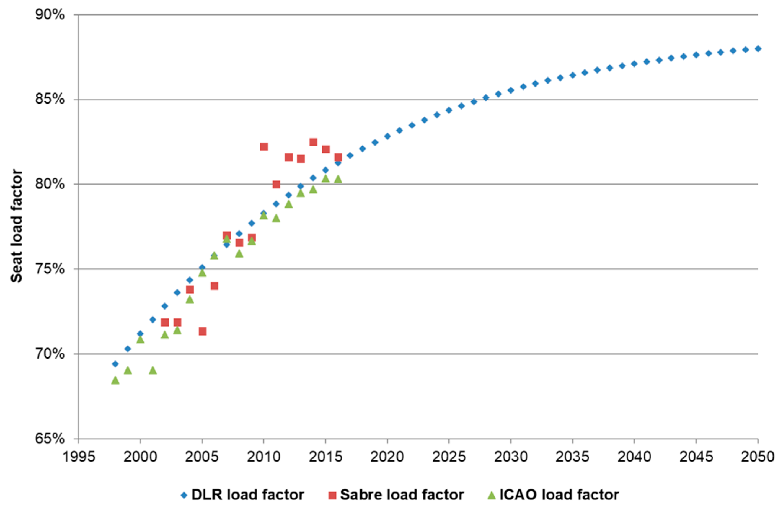
The seat load factor forecast is employed for the conversion of the number of passengers per flight to the number of seats offered. Here, a global model using an s-curve is fitted to empirical data from Sabre AirVision Market Intelligence [27] and ICAO [48,49] using empirical data from 1996 onwards (see Figure 8). From this model, we forecast a maximum seat load factor of 88% in 2050 for all routes.

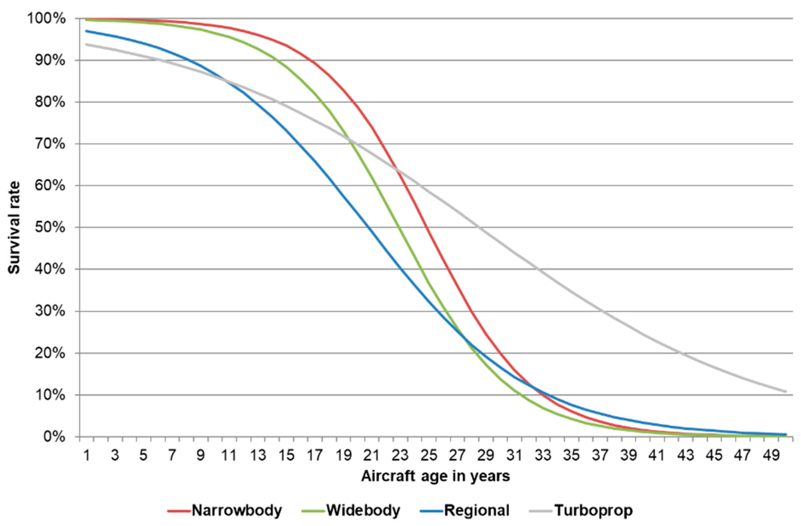
For aircraft retirement modelling, the approach of International Civil Aviation Organization Committee on Aviation Environmental Protection (ICAO CAEP)/12 was employed (see Figure 9). Here, aircraft are subdivided into the following categories: turboprop, regional jet, narrowbody jet and widebody jet. Each type has different coefficients which influence the probability of retirement for a particular aircraft age.

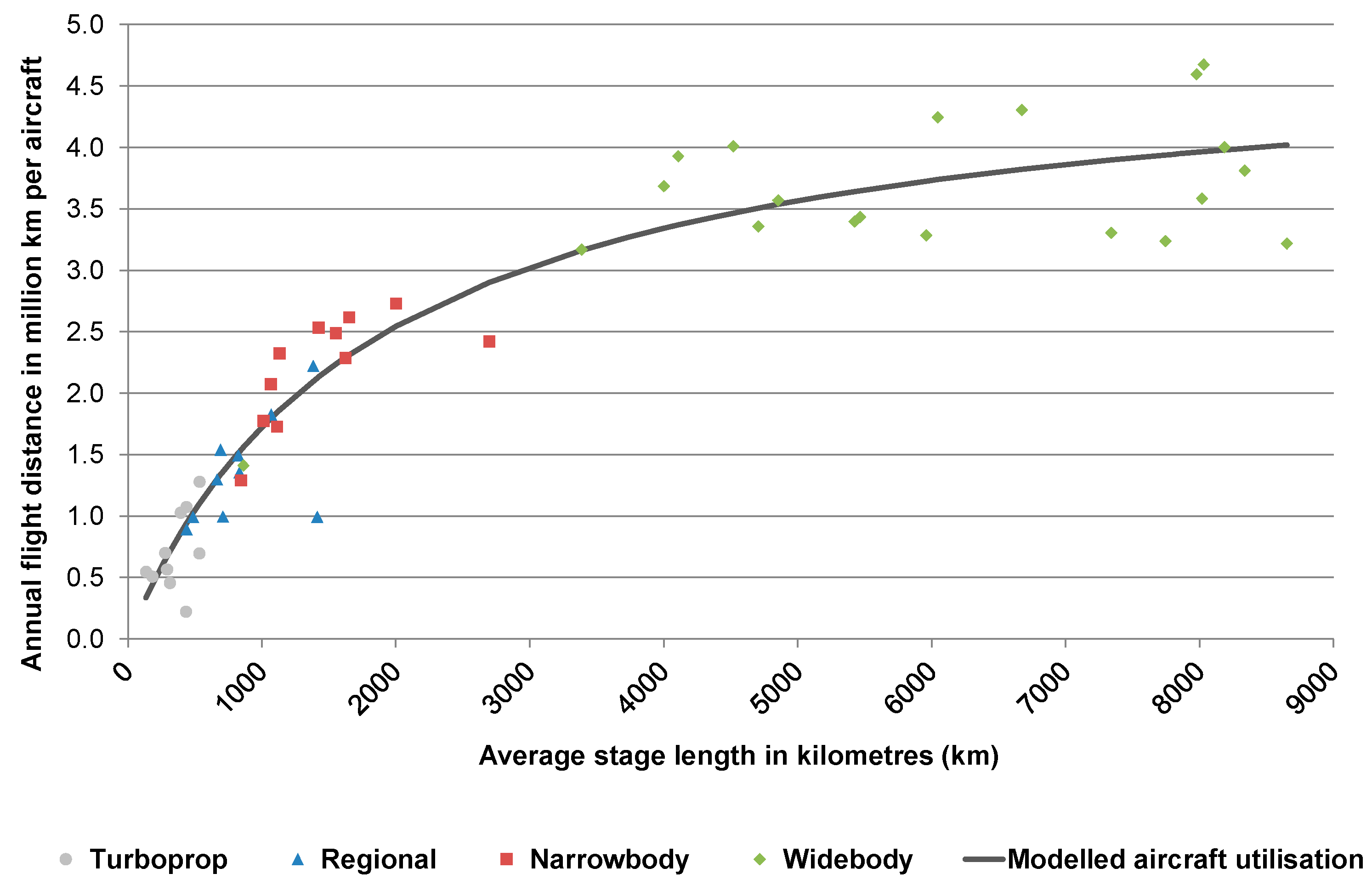
The aircraft utilisation model is needed for the calculation of the number of aircraft that is required to serve the forecast schedule. It is specified as:

$$Utilisation=\frac{a\times Average stage length}{(Average stage length+b)}$$

The total annual aircraft utilisation for each aircraft is estimated by the annual distance flown as a function of the average mission distance with a and b being parameters that are estimated with empirical data. Utilisation typically depends on the average flight length. The longer the flights are, on average, the higher the aircraft utilisation typically is, because the total number of annual turn-arounds with the associated ground times is smaller. The data used to calibrate the model, as shown in Figure 10, originate from ADS-B data collected by Flightradar24 [50] in 2019. ADS-B coverage can be considered to be very high globally, especially because equipage has become mandatory for most operation types. In Europe, about 91% of flights are covered by ADS-B as of early 2022 [51].

The accuracy of the model is shown in

Table 2. Aircraft utilisation model accuracy (data from [45,47]).

Aircraft Type	Active Fleet—Cirium Fleets Analyzer	Estimated Number of Aircraft Based on Innovata Schedule	% Deviation
Airbus A320 Family	7893	7997	1.3%
Airbus A330	1,209	1108	−8.4%
Airbus A340	135	106	−21.3%
Airbus A350	281	315	12.0%
Airbus A380	231	220	−4.6%
ATR 42/72	877	720	−17.9%
Boeing 737	6827	6623	−3.0%
Boeing 747	128	130	1.8%
Boeing 757	352	261	−25.7%
Boeing 767	418	290	−30.6%
Boeing 777	1255	1257	0.2%
Boeing 787	803	836	4.1%
Bombardier CRJ	1227	1078	−12.2%
Embraer E-Series	1397	1378	−1.4%
deHavilland Dash 8	830	639	−23.0%
Total	23,863	22,957	−3.8%

, in which we applied the model to the flight schedule for the year 2019. The model is able to estimate the number of aircraft in the global fleet with an accuracy of 96%. However, forecast results should be taken with a pinch of salt in the case of aircraft-specific deliveries, because there are significant deviations in some cases, e.g., Boeing 757 and 767. A negative value for the deviation means that more aircraft than forecast are needed for a given flight schedule. Nevertheless, in total, i.e., for all aircraft types, this more or less levels out. Furthermore, this only affects deliveries of particular aircraft types but not the total CO₂ and NO_x emissions produced by aircraft in service in this paper. Emissions are calculated by the number of flights per airport pair and aircraft type.

Table 3. Reference aircraft.

Original CS2 Reference Aircaft	ICAO Seat Category	CS2 Reference Aircraft
X	1–19	Do228
	20–50	ATR42-500
X	51–70	CASA C295 Civil (2014 Multi-Mission)
	71–85	Bombardier Dash-8-400
X	86–100	ATR72 Scaled to 90 Seats
	101–125	Embraer E195
X	126–150	Airbus A220-300
	151–175	Airbus A320neo
X	176–210	Airbus A321neo (SMR 2014 ref)
	211–300	Boeing 787-8
X	301–400	Airbus A350-900 (LR 2014 ref)
	401–500	Airbus A380-800 (up to 2021)/Boeing 777-9 (from 2022)

shows the aircraft types used for the Reference Scenario. Only aircraft that were available for order or already in service no later than 2014 are used in the Reference Scenario. They represent state-of-the-art aircraft technology for 2014. Originally, in CS2, only six reference aircraft were included. However, the modelling approach is based upon the 14 ICAO seat classes. The ICAO forecast [15] is one of the leading forecasts in the field, and thus is a point of reference for our study. Furthermore, 14 seat classes are a more appropriate resolution for fleet modelling from our point of view. In order to make the reference aircraft compatible with the modelling approach, additional aircraft were added. In the Reference Scenario, these aircraft are employed during the whole forecasting period from 2014 to 2050. A drawback of the model approach is that aircraft types are assigned permanently to a particular seat category for the full forecast period. Over time, aircraft of an already existing type enter the market, or existing aircraft are upgraded with more seats. The Airbus A320neo is such an example, which was assigned to the 151–175 seats category in 2014, but the aircraft in service hit the upper limit of the class in 2022 [48].

The list of available aircraft in the CS2 Scenario is determined by the environmental goals breakdown table (

Table 4. Clean Sky 2 aircraft type and entry into service.

Conceptual Aircraft/Air Transport Type	Reference Aircraft	Window 1	∆CO2	∆NOx	∆ Noise	Target 2 TRL @ CS2 Close
Advanced Long-range (A-LR)	LR 2014 ref	2030	20%	20%	20%	4
Ultra advanced Long-range (UA-LR)	LR 2014 ref	2035+	30%	30%	30%	3
Advanced Short/Medium-range (A-SMR)	SMR 2014 ref	2030	20%	20%	20%	5
Ultra-advanced Short/Medium-range (UA-SMR)	SMR 2014 ref	2035+	30%	30%	30%	4
Innovative Turboprop (TP), 130 Pax	2014 130 Pax ref	2035+	19 to 25%	19 to 25%	20 to 30%	4
Advanced Turboprop (A-TP), 90 Pax	2014 TP ref	2025+	35 to 40%	>50%	60 to 70%	5
Regional Multi-Mission TP, 70 Pax	2014 Multi-mission	2025+	20 to 30%	20 to 30%	20 to 30%	6
19-Pax Commuter	2014 19 Pax a/c	2025	20%	20%	20%	4-5

¹ All of the key enabling technologies at TRL 6 with a potential entry into service five years later. ² Key enabling technologies at the major system level.

). Aircraft with advanced and ultra-advanced CS2 technologies gradually enter the market according to the entry into service schedule (

Table 5. Overview of the CS2 Scenario aircraft and the in-production window.

Original CS2 Aircraft	Aircraft Scenario Category	ICAO Seat Category	Reference Aircraft	CS2 Aircraft Type	Entry into Service in Forecast Model	Out of Production
x	Reference	1–19	2014 Pax a/c	19-Pax Reference Aircraft	2014	2029
x	CS2	1–19		19-Pax Commuter	2030	2050
	Reference	20–50		ATR42-500	2014	2029
	CS2	20–50		ATR42-500 Advanced	2030	2050
x	Reference	51–70	2014 Multi-Mission	CASA C295 Civil	2014	2029
x	CS2	51–70		Regional Multi-Mission TP 70 seats	2030	2050
	Reference	71–85		Bombardier Dash-8-400	2014	2029
	CS2	71–85		Bombardier Dash-8-400 Advanced	2030	2050
x	Reference	86–100	2014 TP ref	ATR72 Scaled to 90 seats	2014	2029
x	CS2	86–100		Advanced TP90	2030	2050
	Reference	101–125		Embraer E195	2014	2020
	CS2	101–125		Embraer E195–E2	2021	2034
	CS2	101–125		A-SMR-Embraer E195	2035	2039
	CS2	101–125		UA-SMR-Embraer E195	2040	2050
x	Reference	126–150	2014 130 Pax ref	Airbus A220-300	2014	2039
x	CS2	126–150		Innovative Turboprop	2040	2050
	Reference	151–175		Airbus A320neo	2014	2034
	CS2	151–175		A-SMR-Airbus A320neo	2035	2039
	CS2	151–175		UA-SMR-Airbus A320neo	2040	2050
x	Reference	176–210	SMR 2014 ref	Airbus A321neo	2014	2034
x	CS2	176–210		A-SMR	2035	2039
x	CS2	176–210		UA-SMR	2040	2050
	Reference	211–300		Boeing 787-8	2014	2034
	CS2	211–300		A-LR-Boeing 787-8	2035	2039
	CS2	211–300		UA-LR-Boeing 787-8	2040	2050
x	Reference	301–400	LR 2014 ref	Airbus A350-900	2014	2034
x	CS2	301–400		Airbus A350-900neo	2035	2039
x	CS2	301–400		UA-LR	2040	2050
	Reference	401–500		Airbus A380-800	2014	2021
	Reference	401–500		Boeing 777-9	2022	2034
	CS2	401–500		Airbus A350-2000neo	2035	2039
	CS2	401–500		UA-LR	2040	2050

).

As with the reference aircraft, there are only eight original CS2 aircraft classes (see Table 5). In order to fill all of the ICAO seat classes, additional aircraft with similar characteristics to the original CS2 aircraft were introduced. An overview of the aircraft and in-production windows is shown in Table 5.

2.3. Emission Modelling

For the calculation of air transport emissions, various modelling techniques can be employed. In this paper we use the commercial flight performance software Piano-X (Project Interactive Analysis and Optimization) [52] for all reference aircraft for which no emission profiles were provided by the System Platform Developers (SPDs). It is based on the aircraft analysis tool Piano 5, and features flight performance indicators such as fuel burn, CO₂ and NO_x emissions for a set of more than 500 aircraft types. It is widely used in the aviation community, and various studies have validated the accuracy of the tool [53,54]. Generally, the results of calculations using Piano-X have shown a very good alignment with actual fuel consumption and emissions values, as a comparison with the flight data recorder data shows. For CS2 concept aircraft, wherever available, emissions profiles provided by the SPDs were used. In all other cases, reference aircraft with specific reduction factors were employed.

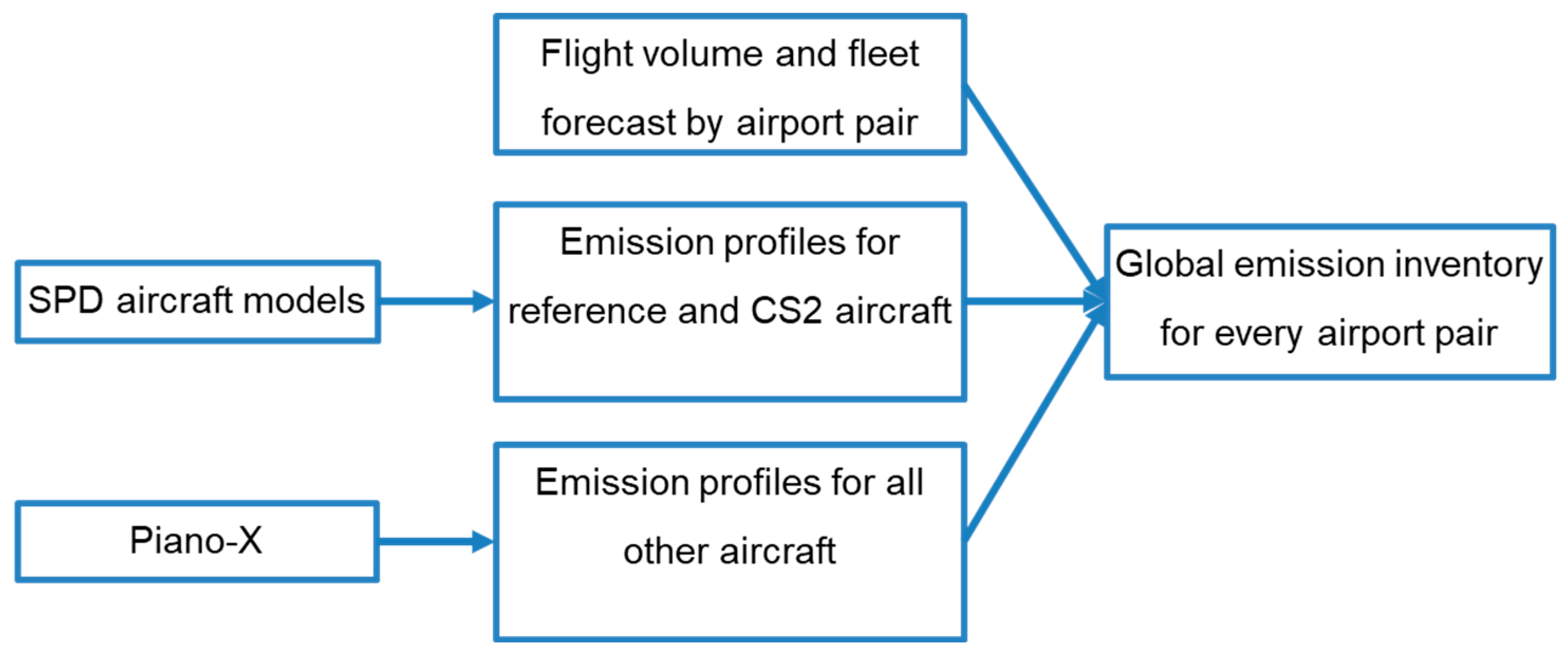
Figure 11 provides an overview of the emissions modelling at the air transport system level. The main inputs are the flight volume and fleet forecast by airport, and the emission profiles from SPD models and Piano-X. The emission profiles are provided by the SPD models and Piano-X. Piano-X is employed for already existing aircraft and the SPD models for the reference and CS2 aircraft. The aircraft models contain encrypted databases from the manufacturers concerning engine thermodynamic and aerodynamic data as well as engine NO_x and fuel flow values. For the calculation of NO_x, the Boeing Fuel Flow Method2 [55] is employed. The aircraft performance module first calculates a trajectory and then the emissions.

The final step is to calculate the global emission inventory using the inputs from the aircraft models for every airport pair.

The main objective of the TE within CS2 is to assess the contribution of aircraft and engine technology to the environmental goals; therefore, we focused on these effects and omitted other contributing factors, which nevertheless play a role in the total fuel consumption and aircraft emissions. For example, we did not consider exact flight routes, but based all of our calculations on great circle distances between origin and destination airports. Any additional distance covered in the terminal maneuvering area around airports, as well as additional cruise distance flown due to detours because of weather, wind or air traffic management restrictions, as well as voluntary detours by airlines in order to save air navigation fees (a typical behavior observed in the EUROCONTROL area, where unit rates can differ substantially in different neighboring countries) are not considered in our analysis. Furthermore, the impact of sub-optimal flight levels or the degradation of aircraft due to age or contamination are not considered. This was to avoid any confounding effects which might negatively influence the identification of aircraft/engine technology effects on emissions.

3. Results

In this section we present the forecast results of:

• the passenger demand and flight volume (Section 3.1).
• the aircraft fleet (Section 3.2).
• the aircraft emissions (Section 3.3).

3.1. Passenger Demand and Flight Volume

Figure 12 displays the results of the passenger demand and flight forecasts. The passenger volume increases on average by 3.9% per year in the High Scenario and 3.3% per year in the Low Scenario. The flight volume rises, on average, by 2.0% per year in the High Scenario and 1.7% per year in the Low Scenario. The difference between the two growth rates, i.e., between passenger and flight volume growth rates, illustrates the increase in the number of passengers per flight. As a result, there is an increase from 109 passengers per flight in 2014 to 214 (1.9% per year) in the High Scenario, and 196 (1.6% per year) in the Low Scenario in 2050. Thus, almost 80% more passengers will be transported per flight in 2050 in the Low Scenario, and 96% more in the High Scenario. In order to manage the passenger volume growth, we have three options:

• we can increase the number of passengers per flight (and hold the numbers of flights constant),
• we can increase the number of flights (and hold the passengers per flight transported constant),
• we can mix both options.

The forecast result is that about 50% of the passenger volume growth is managed by transporting more passengers per flight, and the other 50% is managed by increasing the flight volume. In order to handle more flights, the airport capacity needs to be utilised better and, in some cases, even enlarged. Still, aircraft and airport capacity in 2050 will not be sufficient to avoid any unaccommodated demand: about 7% of passenger demand and 9% of flights will be lost in the High Scenario in 2050 due to capacity constraints. In the Low Scenario, around 4% of the passenger demand and 5% of the flights will be lost in 2050 because of airport capacity shortages.

Furthermore, Figure 12 presents a forecast with a variation of ±1 percentage point of GDP per capita. This illustrates that the forecast is quite sensitive to the GDP per capita assumptions. Because of airport capacity constraints and their impact on flight volume, passenger volume is more sensitive to variations in GDP per capita than flight volume.

Figure 13 shows a comparison of our forecast with the Airbus [56], Boeing [57] and ICAO forecasts [15], which include both domestic and international markets. Those are the leading forecasts in the field, which is the reason why we have chosen them as points of reference. The High Scenario is about 10% lower than the ICAO CAEP/11 forecast. The Airbus and Boeing forecasts are significantly higher: the High Scenario is about 20% lower than the Airbus and Boeing values in 2037 and 2038 as a result of limited airport capacity, which is an aspect which the other three forecasts do not include.

3.2. Aircraft Fleet

Figure 14 displays the fleet forecast by seat class for the Low Scenario, and Figure 15 shows the results for the High Scenario. In both cases we expect a stagnating or even declining regional aircraft market, except for the segment of 86 to 100 seats. For mainliner aircraft, we forecast a substantial shift towards aircraft with more seats, and this tendency is particularly strong in the High Scenario. As a result, we expect the average seats per flight to increase by 1.6% per year in the High Scenario and 1.4% per year in the Low Scenario between 2014 and 2050. By comparison, the seats per flight increased by 1.7% per year between 2000 and 2014 [46].

In the Low Scenario, we forecast a declining importance in terms of aircraft with 101 to 175 seats, and a shift to aircraft with 176 to 500 seats for the mainliner segment. Here, the number of flights with aircraft of 211 to 300 seats, e.g., a Boeing 787–8, grows particularly strong.

In the High Scenario, flight volume with mainliner aircraft of 101 to 175 seats is expected to decline until 2050, while the number of flights with more seats grow in importance. Here, as in the Low Scenario, volume of flights with 211 to 300 seats grows particularly strong. Compared to the Low Scenario, there is a much stronger growth of the number of flights with 301 to 500 seats.

In both scenarios, the shift towards larger aircraft is a result of airlines’ economic considerations and limited airport capacity, especially at large airports which handle a substantial portion of the global flight volume: the largest 120 airports, which correspond to 3% of all airports worldwide with scheduled flights, handle about 50% of the global flight volume. This has not changed significantly since 2000 [2]. However, the shift towards larger aircraft is more pronounced in the High Scenario due to the stronger increase in passenger demand.

Figure 16 compares the forecast of aircraft deliveries until 2038 for the Airbus Global Market Forecast (GMF), which only considers aircraft of over 100 seats, with the results of the High Scenario. According to the Airbus GMF, aircraft are subdivided in three classes: small aircraft have 101 to 210 seats, medium aircraft have 211 to 300 seats, and large aircraft have over 300 seats [56]. Aircraft deliveries are expected to be lower in the High Scenario compared to the Airbus GMF because of the lower number of flights that are forecast (about 30% lower). This is a result of the airport capacity shortage and the related shift to larger aircraft. We expect only about 10,000 new deliveries in the small aircraft class, instead of around 30,000 as predicted by Airbus, but 2400 more in the medium aircraft class and 2900 more in the large aircraft class.

Figure 17 displays the available seat kilometres (ASK) in terms of the technology level in the Low Scenario. As a result of the traffic growth and the replacement of retired aircraft, 52% of the total global ASK will be provided by aircraft with ultra-advanced CS2, and 19% will be provided by aircraft with advanced CS2 technologies in 2050. In total, 29% of the global ASK will be offered by 2014 reference aircraft. Aircraft from the base year and older have almost vanished.

Figure 18 displays the ASK by technology level in the High Scenario. Due to traffic growth and the replacement of retired aircraft, in the year 2050, 56% of the total global ASK will be provided by aircraft with ultra-advanced CS2, and 19% will be provided by aircraft with advanced CS2 technologies. In total, 24% of the global ASKs will be offered by 2014 reference aircraft. Aircraft from the base year and older have virtually vanished. Therefore, in the High Scenario, more CS2 technology aircraft—especially those with ultra-advanced technologies—will be employed in 2050, as there will be more passenger demand, and thus more need for flights.

Figure 19 and Figure 20 display the breakdown of the passenger in-service fleet for the base-year fleet (including reference aircraft already in service in 2014), with replacement and growth for the Low Scenario and High Scenario, respectively.

The surviving base-year fleet and the replacement volume are exactly the same in both scenarios. Naturally, the difference lies in the growth volume, which is substantially larger in the High Scenario due to greater passenger demand leading to a need for more flights. In both scenarios, the base-year fleet has almost vanished in 2050.

3.3. Aircraft Emissions

Table 6. Emission results of the Low and High Scenarios for 2035 to 2050.

Year	High Scenario		Low Scenario
	∆CO2	∆NOx	∆CO2	∆NOx
2035 CS2 vs. Reference	−0.8%	−1.9%	−0.8%	−1.9%
2040 CS2 vs. Reference	−4.6%	−12.0%	−4.1%	−10.2%
2045 CS2 vs. Reference	−10.1%	−23.0%	−9.2%	−20.1%
2050 CS2 vs. Reference	−14.6%	−31.0%	−13.8%	−29.0%

displays the aircraft emission results for the Low and High Scenario for the time period 2035–2050. Here, emission reductions are assessed using a scenario in which CS2 aircraft are introduced over time (Table 5), with a scenario in which only reference aircraft are introduced over time (Table 4). In both the Low and High Scenario there is a substantial reduction of CO₂ and NO_x emissions compared to the corresponding Reference Scenario. The relative emission reduction increases over time, as more and more CS2 aircraft enter service due to demand increasing and older aircraft being retired.

Although there are about 22% more passengers transported and 11% more flights in the High compared to the Low Scenario, the emission reductions compared to the Reference Scenario are very similar in both scenarios. The reason for this is that there is greater traffic growth in the High Scenario, and consequently more CS2 aircraft will be employed until 2050. For example, in the High Scenario, CS2 has a share of around 75% in terms of ASK in 2050, while it is only about 70% in the Low Scenario. As a result, in the High Scenario, there is more traffic because of greater demand, but this is offset by more-advanced and ultra-advanced CS2 aircraft. Overall, CO₂ emissions will be reduced by about 15% and NO_x emissions by around 30% until 2050, compared to the Reference Scenario.

Figure 21 and Figure 22 illustrate the distribution of CO₂ and NO_x emissions by the Airbus seat classes (see also Figure 16) and flight distance, as well as the share of flights and revenue passenger kilometres (RPK) for each distance band and seat class, respectively. The results are virtually the same for both the Low and High Scenario. In 2050, about 55% of CO₂ and NO_x emissions will be from the flights of medium (211–300 seats) and large (over 300 seats) aircraft, on flights of less than 4000 km. In 2020, this share was only about 20%, and in 2014 it was around 10%. If we look at flights of up to 2000 km, medium and large aircraft account for 35% of CO₂ and 36% of NO_x emissions in 2050. The reason for this development is the substantial increase in passenger demand, and the related growth of aircraft size, i.e., passengers and seats per flight, especially on rather short routes.

4. Discussion and Conclusions

When considering the two scenarios, the technological (and thus the demand) development is much more favorable in the High Scenario, in which passenger demand increases by 297% and flight volume increases by 102% between 2014 and 2050, while in the Low Scenario, passenger demand rises by 227% and flight volume rises by 82%. The difference between the passenger and flight volume development illustrates that there is a substantial increase in the number of passengers per flight until 2050 in both scenarios, and therefore a strong tendency to employ larger aircraft in the future.

Over time, there will be a constant shift towards bigger aircraft, with the class of 211 to 300 seats being the most important in terms of flights in 2050. Larger aircraft with up to 500 seats are becoming more important as well, especially in the High Scenario, because of the stronger passenger demand development. The number of seats per flight is expected to increase by 1.6% per year in the High Scenario and 1.4% per year in the Low Scenario.

However, due to the CS2 aircraft which enter into service over time as older aircraft are replaced and additional new aircraft are needed because of the increasing passenger demand, there will be a considerable drop in CO₂ and NO_x emissions compared to the Reference Scenario, in which only aircraft from 2014 or older are employed: in both scenarios, CO₂ emissions can be reduced by about 15% and NO_x emissions can be reduced by around 30% until 2050 compared to the Reference Scenario. Despite the substantial difference in passenger and flight volumes between the two scenarios, the emission results of the High Scenario are even better than those of the Low Scenario, as more-advanced and ultra-advanced CS2 aircraft will have entered into service due to the higher level of passenger demand and flight volume. This is a very important result; it shows the environmental potential of CS2 aircraft. Nevertheless, in 2050, medium (211–300 seats) and large (over 300 seats) aircraft will produce a substantial share of their CO₂ and NOx emissions on flights of up to 2000 km. This is essentially a result of the large increase of passenger demand volume on rather short routes, which is not optimal for medium and large aircraft. This naturally raises a question about the development of a large-capacity aircraft for short- and medium-distance flights, say of up to 3000 or 4000 km.

Nevertheless, there are of course some serious limitations of the study, such that further research is needed. First, the effects of the COVID-19 pandemic are not considered. The pandemic might have an effect on the long-term travel behaviour of leisure as well as business passengers, such that future demand development will be different compared to this study. Furthermore, there is uncertainty about when air traffic volume will have been recovered to pre-pandemic levels. First analyses have already been conducted [7] and will be part of an update of this study.

Another limitation of the study is that there is no differentiation between business and leisure travellers. This is because of a lack of consistent global data on the share of business and leisure travellers. Recent trends, like virtual meetings, which have been more and more established during the COVID-19 pandemic, might continue after the pandemic to some degree, and thus might influence the need for business travel.

In our model, aircraft types are assigned to particular seat classes for the whole forecast period and cannot switch to another class. However, we have observed that aircraft of an already existing type can enter the market with more seats, or aircraft which are already in service can be upgraded. The Airbus A320neo is such an example: it is assigned to the 151–175 seats category in 2014, but aircraft in service already hits the upper limit of the class in 2022 [48]. While this seems to be more of a relatively minor limitation of the study, it is an area where the model can be improved. However, it is a challenge to anticipate seat capacity upgrades of existing aircraft, and to differentiate between whether such an upgraded aircraft or an already existing aircraft with larger seat capacity is employed. This is an issue in which complexity quickly increases.

Lastly, the approach to model multi-airport regions like London Heathrow and their potential to mitigate capacity constraints needs to be improved. This has an effect on the air passenger demand level, and in the course of this on aircraft fleet composition. However, based on our research so far, we do not expect this to have a major influence on demand level, as airlines seem to prefer to increase the number of passengers per flight instead of shifting flights to neighbour airports. This can be achieved by fitting more seats in existing aircraft or employing larger aircraft. Employing larger aircraft is not only about very large aircraft like the Airbus A380 (which is out of production now) or the Boeing 777–9 but also about employing larger aircraft step-by-step across the whole range from small to large aircraft. Here, aircraft in the range of about 211 to 300 seats play a particularly important role, like the Airbus A321neo or the Boeing 787–8. On the other hand, we see some potential for more nonstop long-haul connections with the introduction of smaller, efficient, long-haul aircraft like the Airbus A321XLR [58,59].

These limitations should be taken seriously, and naturally raise the question about the benefits of this study. Despite the need for improvements, we have shown that the model developed can assess the environmental benefits of aircraft technology end-to-end, i.e., from the generation of air passenger demand to aircraft fleet modelling, and finally emissions modelling. A particular strength is the bottom-up approach, i.e., the approach is based on airport pairs instead of larger aggregates, which enables the consideration of airport capacity constraints.

Furthermore, the study provides a first overview of the environmental benefit of CS2 technology. Additional technical improvements will be considered in the second (and final) assessment in 2024. The COVID-19 pandemic-related limitations are expected to lower future passenger and flight volume, and thus the overall environmental impact of aviation, but this does not change the benefit of CS2 technology substantially.

References

1. Berster, P.; Gelhausen, M.C.; Wilken, D. Is increasing aircraft size common practice of airlines at congested airports? J. Air Transp. Manag. 2015, 46, 40–48. [Google Scholar] [CrossRef]
2. Gelhausen, M.C.; Berster, P.; Wilken, D. Airport Capacity Constraints and Strategies for Mitigation: A Global Perspective; Academic Press: New York, NY, USA, 2019; pp. 1–327. [Google Scholar]
3. Wilken, D.; Berster, P.; Gelhausen, M.C. New empirical evidence on airport capacity utilisation: Relationships between hourly and annual air traffic volumes. Res. Transp. Bus. Manag. 2011, 1, 118–127. [Google Scholar] [CrossRef] [Green Version]
4. Givoni, M.; Rietveld, P. The environmental implications of airlines’ choice of aircraft size. J. Air Transp. Manag. 2010, 16, 159–167. [Google Scholar] [CrossRef]
5. Pitfield, D.E.; Caves, R.E.; Quddus, M.A. Airline strategies for aircraft size and airline frequency with changing demand and competition: A simultaneous-equations approach for traffic on the north Atlantic. J. Air Transp. Manag. 2010, 16, 151–158. [Google Scholar] [CrossRef] [Green Version]
6. Brueckner, J.K.; Zhang, Y. A model of scheduling in airline networks: How a hub-and-spoke system affects flight frequency, fares and welfare. J. Transp. Econ. Policy 2001, 35, 195–222. [Google Scholar]
7. Gelhausen, M.C.; Berster, P.; Wilken, D. Post-COVID-19 Scenarios of Global Airline Traffic until 2040 That Reflect Airport Capacity Constraints and Mitigation Strategies. Aerospace 2021, 8, 300. [Google Scholar] [CrossRef]
8. Gelhausen, M.C. Modelling the effects of capacity constraints on air travellers’ airport choice. J. Air Transp. Manag. 2011, 17, 116–119. [Google Scholar] [CrossRef]
9. Gudmundsson, S.V.; Paleari, S.; Redondi, S. Spillover effects of the development constraints in London Heathrow Airport. J. Transp. Geogr. 2014, 35, 64–74. [Google Scholar] [CrossRef]
10. Redondi, R.; Gudmundsson, S.V. Congestion spill effects of Heathrow and Frankfurt airports on connection traffic in European and Gulf hub airports. Transp. Res. Part A Policy Pract. 2016, 92, 287–297. [Google Scholar] [CrossRef]
11. Dennis, N. Airline hub operations in Europe. J. Transp. Geogr. 1994, 2, 219–233. [Google Scholar] [CrossRef]
12. Airports Commission. Airports Commission: Final Report; Airports Commission: London, UK, 2015. [Google Scholar]
13. Airbus. Global Market Forecast 2021–2040; Airbus: Blagnac, France, 2021. [Google Scholar]
14. Boeing. Commercial Market Outlook 2021–2040; Boeing: Seattle, WA, USA, 2021. [Google Scholar]
15. International Civil Aviation Organization (ICAO). ICAO Long-Term Traffic Forecast—Passenger and Cargo; ICAO: Montreal, QC, Canada, 2016. [Google Scholar]
16. Harvey, D. Airline passenger traffic patterns within the United States. J. Air Law Commer. 1951, 18, 157–165. [Google Scholar]
17. Grosche, T.; Rothlauf, F.; Heinzl, A. Gravity models for airline passenger volume estimation. J. Air Transp. Manag. 2007, 13, 175–183. [Google Scholar] [CrossRef]
18. Tusi, W.H.K.; Fung, M.K.Y. Analysing passenger network changes: The case of Hong Kong. J. Air Transp. Manag. 2016, 50, 1–11. [Google Scholar]
19. Matsumoto, H. International urban systems and air passenger and cargo flows: Some calculations. J. Air Transp. Manag. 2004, 10, 241–249. [Google Scholar] [CrossRef] [Green Version]
20. Shen, G. Reverse-fitting the gravity model to inter-city airline passenger flows by an algebraic simplification. J. Transp. Geogr. 2004, 12, 219–234. [Google Scholar] [CrossRef]
21. Bhadra, D.; Kee, J. Structure and dynamics of the core US air travel markets: A basic empirical analysis of domestic passenger demand. J. Air Transp. Manag. 2008, 14, 27–39. [Google Scholar] [CrossRef]
22. Endo, N. International trade in air transport services: Penetration of foreign airlines into Japan under the bilateral aviation policies of the US and Japan. J. Air Transp. Manag. 2007, 13, 285–292. [Google Scholar] [CrossRef]
23. Hazledine, T. Border effects for domestic and international Canadian passenger air travel. J. Air Transp. Manag. 2009, 15, 7–13. [Google Scholar] [CrossRef]
24. Alexander, D.W.; Merkert, R. Challenges to domestic air freight in Australia: Evaluating air traffic markets with gravity modelling. J. Air Transp. Manag. 2017, 61, 41–52. [Google Scholar] [CrossRef]
25. Alexander, D.W.; Merkert, R. Applications of gravity models to evaluate and forecast US international air freight markets post-GFC. Transp. Policy 2021, 104, 52–62. [Google Scholar] [CrossRef]
26. Baier, F.; Berster, P.; Gelhausen, M.C. Global cargo gravitation model: Airports matter for forecasts. Int. Econ. Econ. Policy 2022, 19, 219–238. [Google Scholar] [CrossRef]
27. Sabre AirVision Market Intelligence. Data Based on Market Information Data Tapes (MIDT). Available online: https://www.sabre.com/products/market-intelligence/ (accessed on 8 November 2021).
28. Silva, J.M.C.S.; Tenreyro, S. The log of gravity. Rev. Econ. Stat. 2006, 88, 641–658. [Google Scholar] [CrossRef] [Green Version]
29. Wilken, D.; Berster, P.; Gelhausen, M.C. Airport choice in Germany: New empirical evidence of the 2003 German air traveller survey. Airpt. Manag. 2007, 1, 165–179. [Google Scholar]
30. Mason, K.J. Corona Markiert Eine Zäsur Bei Geschäftsreisen. Available online: https://www.airliners.de/airline-geschaeftsmodelle-88-corona-markiert-zaesur-geschaeftsreisen/61658 (accessed on 23 August 2021).
31. Charnes, A.; Cooper, W.W.; Rhodes, E. Measuring the efficiency of decision-making units. Eur. J. Oper. Res. 1978, 2, 429–444. [Google Scholar] [CrossRef]
32. Cooper, W.W.; Seiford, L.M.; Tone, K. Data Envelopment Analysis—A Comprehensive Text with Models, Applications, References and DEA-Solver Software; Springer: New York, NY, USA, 2007. [Google Scholar]
33. Markov, A.A. An Example of Statistical Investigation of the Text Eugene Onegin Concerning the Connection of Samples in Chains. Sci. Context 2006, 19, 591–600. [Google Scholar] [CrossRef] [Green Version]
34. McFadden, D. Conditional Logit Analysis of Qualitative Choice Behavior. In Frontiers in Econometrics; Zarembka, P., Ed.; Academic Press: New York, NY, USA, 1974. [Google Scholar]
35. Ben-Akiva, M.; Lerman, S.R. Discrete Choice Analysis; MIT Press: Cambridge, MA, USA, 1985. [Google Scholar]
36. Gelhausen, M.C.; Berster, P.; Wilken, D. Do airport capacity constraints have a serious impact on the future development of air traffic? J. Air Transp. Manag. 2013, 28, 3–13. [Google Scholar] [CrossRef]
37. Wei, W.; Hansen, M. Impact of aircraft size and seat availability on airlines’ demand and market share in duopoly markets. Transp. Res. Part E Logist. Transp. Rev. 2005, 41, 315–327. [Google Scholar] [CrossRef]
38. Presto, F.; Gollnick, V.; Lütjens, K. Fleet upgauging and reducing flight frequency. J. Air Transp. 2022, 30, 23–36. [Google Scholar] [CrossRef]
39. Kölker, K.; Bießlich, P.; Lütjens, K. From passenger growth to aircraft movements. J. Air Transp. Manag. 2016, 56, 99–106. [Google Scholar] [CrossRef]
40. Givoni, M.; Rietveld, P. Airline’s choice of aircraft size—Explanations and implications. Transp. Res. Part A 2009, 43, 500–510. [Google Scholar] [CrossRef]
41. Bhadra, D. Choice of aircraft fleets in the U.S. domestic scheduled air transportation system: Findings from a multinomial logit analysis. J. Transp. Res. Forum 2005, 44, 143–162. [Google Scholar] [CrossRef]
42. Pai, V. On the factors that affect airline flight frequency and aircraft size. J. Air Transp. Manag. 2010, 16, 169–177. [Google Scholar] [CrossRef] [Green Version]
43. Bhadra, D. Choice of aircraft fleets in the US NAS: Findings from a multinomial logit analysis. In Proceedings of the 3rd AIAA Aviation Technology, Integration, and Operations Conference, Denver, CO, USA, 17–19 November 2003. [Google Scholar]
44. Bhadra, D. Demand for Air Travel in the United States: Bottom-Up Econometric Estimation and Implications for Forecasts by Origin-Destination Pairs. In Proceedings of the 2nd AIAA Aviation Technology, Integration, and Operations Conference, Los Angeles, CA, USA, 1–3 October 2002. [Google Scholar]
45. Cirium. Fleets Analyzer. Available online: https://www.cirium.com/products/views/fleets-analyzer/ (accessed on 8 November 2021).
46. Official Airline Guide (OAG). Flight Schedules. Available online: https://www.oag.com/ (accessed on 8 November 2021).
47. Flightglobal. Innovata Flight Schedules. Available online: https://www.flightglobal.com/ (accessed on 8 November 2021).
48. International Civil Aviation Organization (ICAO). Annual Report of the Council (Doc 9916). 2009. Available online: https://www.icao.int/publications/Documents/9916_en.pdf (accessed on 22 February 2022).
49. International Civil Aviation Organization (ICAO). Annual Report of the Council, Presentation of 2016 Air Transport Statistical Results. 2017. Available online: https://www.icao.int/annual-report-2016/Pages/the-world-of-air-transport-in-2016-statistical-results.aspx (accessed on 22 February 2022).
50. Flightradar24. Live Air Traffic. Available online: https://www.flightradar24.com/50.83,6.91/6 (accessed on 8 November 2021).
51. Eurocontrol. Automatic Dependent Surveillance–Broadcast Airborne Equipage Monitoring. Available online: https://www.eurocontrol.int/service/adsb-equipage (accessed on 22 February 2022).
52. Lissys. Piano-X. Available online: https://www.lissys.uk/PianoX.html (accessed on 8 November 2021).
53. Dons, J.; Mariens, J.; O’Callaghan, G.D. Use of Third-Party Aircraft Performance Tools in the Development of the Aviation Environmental Design Tool (AEDT); Report of the U.S. Department of Transportation, Research and Innovative Technology Administration; John A. Volpe National Transportation Systems Center, Environmental Measurement and Modeling Division: Washington, NJ, USA, 2011.
54. Senzig, D.A.; Dons, J.; Mariens, J.; O’Callaghan, G.D.; Iovinelli, R.J. Extending Aircraft Performance Modeling Capabilities in the Aviation Environmental Design Tool (AEDT); Report of the John A. Volpe National Transportation Systems Center; Federal Aviation Administration—Office of Environment and Energy: Washington, NJ, USA, 2011.
55. DuBois, D.; Paynter, G.C. Fuel Flow Method2 for estimating aircraft emissions. SAE Int. J. Aerosp. 2006, 115, 1–14. [Google Scholar]
56. Airbus. Global Market Forecast 2019–2038; Airbus: Blagnac, France, 2019. [Google Scholar]
57. Boeing. Commercial Market Outlook 2019–2038; Boeing: Seattle, WA, USA, 2019. [Google Scholar]
58. Grimme, W.; Maertens, S.; Bingemer, S.; Gelhausen, M.C. Estimating the market potential for long-haul narrowbody aircraft using origin-destination demand and flight schedules data. Transp. Res. Procedia 2021, 52, 412–419. [Google Scholar] [CrossRef]
59. Wilken, D.; Berster, P.; Gelhausen, M.C. Analysis of demand structures on intercontinental routes to and from Europe with a view to identifying potential for new low-cost services. J. Air Transp. Manag. 2016, 56B, 79–90. [Google Scholar] [CrossRef]
Figure 1. Overview of the passenger and flight forecast model.
Aerospace 09 00204 g001
Figure 2. Relationship between passenger demand, airport capacity and aircraft size. Reprinted from Ref. [7].
Aerospace 09 00204 g002
Figure 3. Relative development of passenger volume and aircraft movements at airports in the London area between 2006 and 2019 (2006 = 100). Reprinted from Ref. [7].
Aerospace 09 00204 g003
Figure 4. Elasticities of air passenger demand. Reprinted from Ref. [7].
Aerospace 09 00204 g004
Figure 5. Estimation of the generic airport capacity model.
Aerospace 09 00204 g005
Figure 6. Markov chain of runway expansion.
Aerospace 09 00204 g006
Figure 7. Forecasting the passengers per aircraft for each airport pair.
Aerospace 09 00204 g007
Figure 8. Seat load factor data and forecast [27,48,49].
Aerospace 09 00204 g008
Figure 9. Survival probabilities of aircraft in relation to the aircraft category and age.
Aerospace 09 00204 g009
Figure 10. Aircraft utilisation model.
Aerospace 09 00204 g010
Figure 11. Overview of air transport system level emissions calculation.
Aerospace 09 00204 g011
Figure 12. Results of the passenger demand and flight volume forecast.
Aerospace 09 00204 g012
Figure 13. Comparison with the Airbus, Boeing and ICAO forecasts.
Aerospace 09 00204 g013
Figure 14. Fleet forecast results in the Low Scenario.
Aerospace 09 00204 g014
Figure 15. Fleet forecast results in the High Scenario.
Aerospace 09 00204 g015
Figure 16. Comparison of the aircraft deliveries forecast of the Airbus GMF and the High Scenario forecast for the time period 2019–2038.
Aerospace 09 00204 g016
Figure 17. Available seat kilometres (ASK) by technology level in the Low Scenario. The grey, blue, red and green bars add up to the total ASK volume for the respective year.
Aerospace 09 00204 g017
Figure 18. Available seat kilometres (ASK) by technology level in the High Scenario. The grey, blue, red and green bars add up to the total ASK volume for the respective year.
Aerospace 09 00204 g018
Figure 19. Passenger-in service fleet breakdown in the Low Scenario.
Aerospace 09 00204 g019
Figure 20. Passenger-in service fleet breakdown in the High Scenario.
Aerospace 09 00204 g020
Figure 21. Distribution of CO2 emissions by seat class and flight distance in 2050.
Aerospace 09 00204 g021
Figure 22. Distribution of NOx emissions by seat class and flight distance in 2050.
Aerospace 09 00204 g022