1. Introduction
Numerical prediction of the broadband noise from a subsonic turbulent jet remains a challenge for Computational Aeroacoustics (CAA) due to the need to resolve a wide range of disparate spatial and temporal scales. Furthermore, the scale disparity between the fluid dynamic and acoustic disturbances requires greater numerical accuracy to prevent high frequencies from being damped by dissipation inherent in the numerical schemes [
1]. With computational fluid dynamics (CFD), resolving the smallest turbulence scales needed for acoustic predictions drastically increases the computational cost. In fact, resolution of all the turbulent scales via direct numerical simulation (DNS) for a moderately high Reynolds number jet is not currently feasible due to the extreme cost.
The current standard for CFD-based jet simulations is large-eddy simulation (LES). Recent advances in simulation methodology, such as wall modeling for the nozzle interior boundary layer [
2], have led to more reliable LES predictions (often at flight Reynolds numbers), and application to more complicated problems [
3,
4,
5,
6]. Despite these improvements, the problem still remains that LES is computationally expensive yet still cannot resolve high-frequency acoustic disturbances [
3,
4,
7,
8,
9]. Since LES only resolves the large turbulent scales (which generate low-frequency noise [
10]), modeling is required for the smallest turbulent scales that cannot be resolved by the computational grid. Subgrid-scale (SGS) models for LES do not generate acoustics that correspond to these modeled small scales, which leads to the problem of missing high-frequency content. Increasing the grid resolution to resolve small scales drives up the expense exponentially, making LES impractical for industrial use [
11]. Present-day LES simulations can accurately resolve frequencies up to Strouhal numbers of 3 to 5 (St =
) [
4], although St = 7 has been reported recently [
6]. This range does not even account for all of the high-frequency content in the jet noise spectra, which can extend up to St = 30 [
9,
12,
13].
For subsonic jet noise, it is important to note that the frequency content varies with the observer angle to the jet [
10]. This spectral directivity arises in part due to two separate source mechanisms for subsonic jet noise [
10,
14,
15,
16,
17,
18]. Large coherent eddies and turbulent structures near the end of the potential core generate low-frequency noise, which radiates primarily in the downstream direction. This low-frequency noise dominates the jet noise spectra, comprising the majority of observed sound from a subsonic jet.
A second, less intense sound source arises from small-scale turbulent eddies mixing randomly in the shear layer. Fine-scale mixing generates broadband noise (including high frequencies [
10,
19,
20]) that radiates nearly uniformly. The strength of low-frequency noise at downstream angles renders high-frequency noise insignificant at those observation locations. However, high-frequency noise becomes more influential at sideline angles (90°), where low frequencies do not dominate the spectra [
15,
20,
21]. A more thorough review of possible noise mechanisms for these two sources and their locations within the jet can be found in Blake [
22].
For full-scale jets, the high frequencies produced by small-scale turbulence can correspond to the frequency range most annoying to humans and cannot fully be ignored [
9,
15,
23]. From the previous discussion, jet noise predictions based on LES simulations cannot resolve high frequencies and, therefore, under-predict a less intense yet important portion of the jet noise spectra. The inability of LES to resolve a full noise spectrum in a cost-effective manner suggests the need for an alternative method for LES-based noise prediction, such as a model for the missing high-frequency noise.
Several authors have investigated different approaches for modeling the missing high-frequency noise content. Seror et al. [
24] apply both a priori and a posteriori methods to filtered DNS results of isotropic turbulence in order to evaluate a hybrid LES/Lighthill noise prediction approach. They observed that the noise from unresolved turbulent scales (or residual SGS stresses) is essential to predict the full acoustic spectra. Batten et al. [
25,
26] combine resolved fluctuations from LES and subgrid fluctuations from a statistical, Fourier-mode model to generate noise sources. Bodony and Lele [
7] develop equations to model the velocity and pressure arising from the missing subgrid scales, using an acoustic analogy approach. Their method is based on the idea that interaction between resolved and missing scales is important to account from the noise arising from the missing scales. Bodony and Lele [
11] further developed this method into a statistical noise model for source terms corresponding to the missing noise, relating the space-time correlations of the source terms to the far-field power spectral density of the fluctuating density, obtaining the far-field noise by an adjoint formulation of Goldstein’s generalized acoustic analogy. Independently, Bodony [
9] uses a Gabor transform to derive equations that approximate the behavior of the subgrid turbulent scales above a cut-off frequency wave number. Additionally, a Lagrangian particle approach estimates subgrid fluctuations and reconstructs the Reynolds stress contributions from the modeled subgrid scales. The subgrid stresses, once obtained, can then be used with an acoustic analogy to form noise source terms for the subgrid turbulence. Unfortunately, the work only presented the method and did not show results.
The most relevant literature on this topic is a paper by Yao and He [
27], who propose the use of synthetic fluctuations to account for the missing LES noise content. They apply the kinematic simulation (KS) method of Fung et al. [
28] to model subgrid-scale fluctuations that are not resolved by LES, taking care to match both time and space statistics in order to account for the random sweeping hypothesis [
29,
30]. A hybrid CAA method is used to compute noise by Lighthill’s acoustic analogy. Comparisons with DNS for isotropic turbulence show that a combination of LES and synthetic fluctuations can approximately recover the high-frequency content missing from the noise spectra. However, this method was not applied to more complex flows and cannot be used for turbulent shear flows (i.e., jets) because their implementation of the sweeping hypothesis does not account for the influence of the unsteady resolved fluctuations on the unresolved, modeled fluctuations.
The work of Yao and He [
27] shows the possibility for synthetic turbulence methods to model the missing high frequencies from LES-predicted noise spectra in general. While several different approaches have been taken to solve the missing noise problem, none have shown results for jet noise prediction. With regards to synthetic turbulence methods, several authors have investigated the use of SEM to model jet noise [
31,
32].
Fukushima [
31] modify the Stochastic Noise Generation and Radiation (SNGR) method (a synthetic turbulence method built on the summation of Fourier modes [
33]) to use the synthetic eddy method (SEM) to model turbulent fluctuations in the jet shear layer via a superposition of eddies instead of a superposition of Fourier modes. The SEM method was proposed by Jarrin et al. [
34] as a simple and computationally inexpensive method to generate more-realistic turbulence inflow conditions for homogeneous isotropic LES simulations [
34,
35,
36]. Synthetic eddy methods allow locally-specified length scales and turbulent properties and therefore respond better to local stretching and deforming, which is ideal for the sweeping and straining of turbulence present in jet shear layers. A Reynolds-averaged Navier–Stokes (RANS)-generated background shear flow is used by Fukushima [
31] and the Linearized Euler equations (LEE) with source terms are used to propagate the synthetically-generated noise sources.
The method of Hirai et al. [
32] shows promise for the use of SEM methods in jet noise prediction, building on the work of Fukushima [
31] by investigating the statistical properties of the synthesized turbulent velocity field. Hirai et al. introduce a turbulence dissipation mechanism (a time-decorrelation process) that modulates the intensity of each eddy in time to better match the temporal decorrelation observed in the experimental data of Fleury et al. [
37]. This is needed because the original SEM method (by Jarrin et al. [
34]) does not correctly model the dissipation of turbulent structures in time. In the method by Hirai et al. [
32], each eddy is convected by a constant mean flow velocity. The size and strength of each eddy are recalculated in time based on convection and the background RANS field TKE and
. The authors reported significantly over-predicting the jet noise when the model was first tuned to match the spatial and temporal statistics of the turbulent flowfield. The noise spectra was only matched when the turbulent properties of the synthetic field were adjusted. However, their results show that SEM-based methods can be used for jet noise predictions.
Given the highlighted issues with current LES approaches and the potential of SEM-based methods to model jet noise, the coupled LES-synthetic turbulence (
CLST) method is presented to supplement the missing high-frequency noise for LES-based jet noise predictions. The
CLST method is based on the assumption that the unresolved small-scale turbulence are isotropic and can therefore be modeled sufficiently by randomized synthetic turbulence rather than developing a model from first principles. In contrast to the methods of Fukushima [
31] and Hirai et al. [
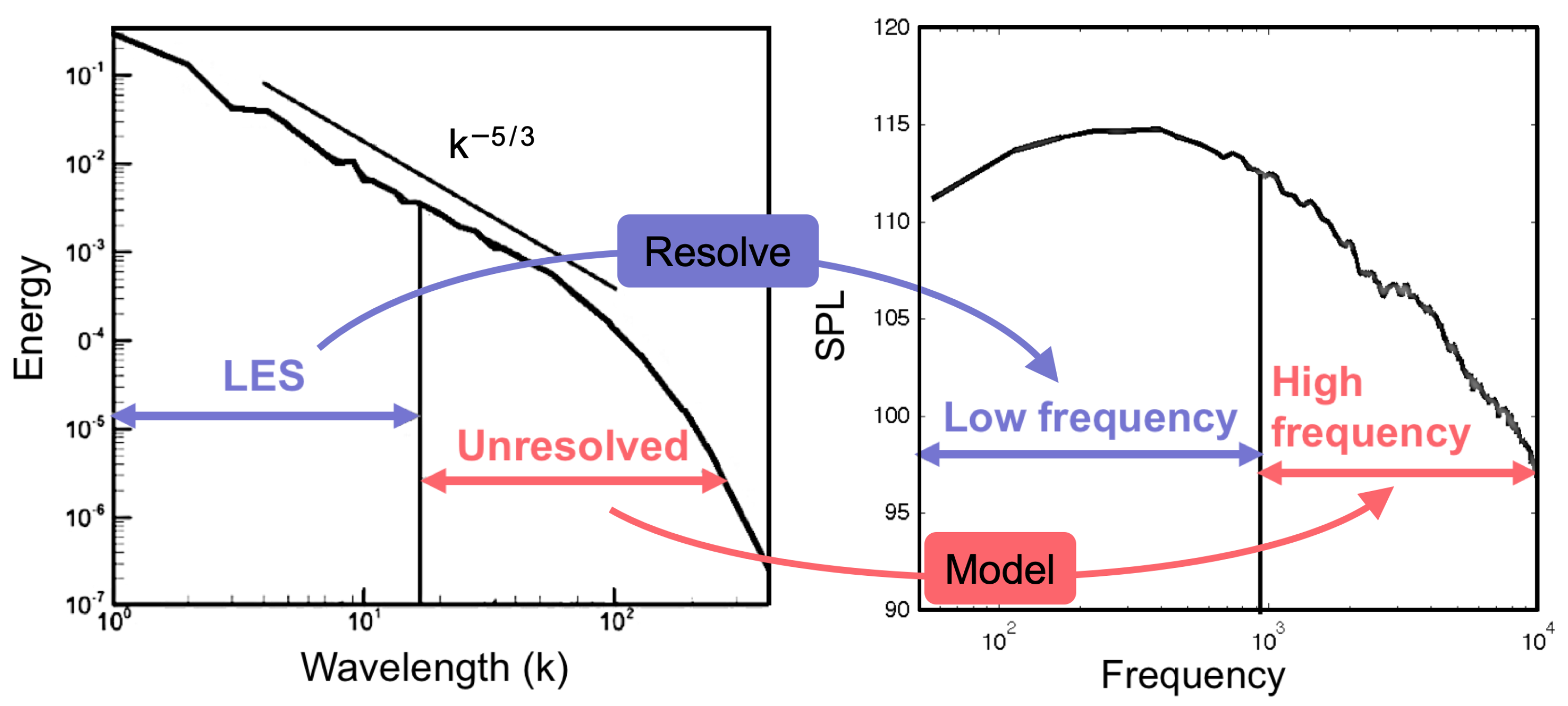
32], the CLST method resolves large turbulent fluctuations (corresponding to low-frequency acoustic waves) with LES or CLES (coarse-grid large-eddy simulations) for the mean flow and generates small turbulent fluctuations (corresponding to high-frequency acoustic waves) with synthetic turbulence modeling. A representation of the process is shown in
Figure 1. The resulting resolved and modeled fluctuations are combined and are used to generate noise sources, which are then propagated with a linearized Euler equation (LEE) solver in a hybrid CAA method. By design, the CLST method convects small-scale synthetic eddies by the resolved, large-scale velocities from LES or CLES, which accounts for sweeping and distortion of the small turbulent scales by the large turbulent scales [
38,
39,
40,
41,
42].
The primary goal of this work is to present a model for the high-frequency spectral content that is missing from LES far-field jet noise predictions and to demonstrate that the CLST method can correctly model near-field jet noise spectra. Such an approach has already shown promise with an SNGR-based turbulence model [
43]. A secondary goal of the
CLST method is to reduce overall LES simulation costs while still maintaining a high level of fidelity. A cost reduction is possible when using a less-dense spatial grid resolution (CLES) to model the jet. Further cost reduction is possible when using the LEE to propagate noise instead of the Navier–Stokes (NS) equations because the LEE are a simplified equation set and are cheaper to solve on a given grid. Additionally, with an LEE solver, a coarser grid resolution can be used outside the jet source region while still resolving the necessary acoustic spectrum. LEE can also be extended to the far-field for a cheaper cost than the NS equations. Of course, alternative methods for acoustic propagation, such as a permeable Ffowcs–Williams and Hakwings formulation, Kirchoff’s method, or Lighthill’s acoustic analogy could be used. However, LEE is chosen for the
CLST method because the acoustic source terms come directly from velocity fluctuations, making it simple to add the contributions of velocity fluctuations generated by synthetic eddies.
Predicting a more-complete noise spectrum and reducing simulation costs should lead to equally reliable results in a shorter amount of time, potentially allowing the use of LES jet noise predictions more readily in research and industry. This might enable quicker design cycles or the inclusion of wing and pylon installation effects in LES jet noise simulations, as is suggested might soon be possible for business jets [
13]. Overall, the
CLST method will provide a new framework for LES predictions of turbulence-related noise mechanisms.
This work introduces the CLST method and details the implementation of CLST with SEM-generated fluctuations. The CLST method is applied to a moderately high Reynolds number, Mach 0.9 jet to investigate the effectiveness supplementing the missing high-frequency portion of the jet noise spectra.
2. Problem Formulation and Numerical Framework
2.1. Overview
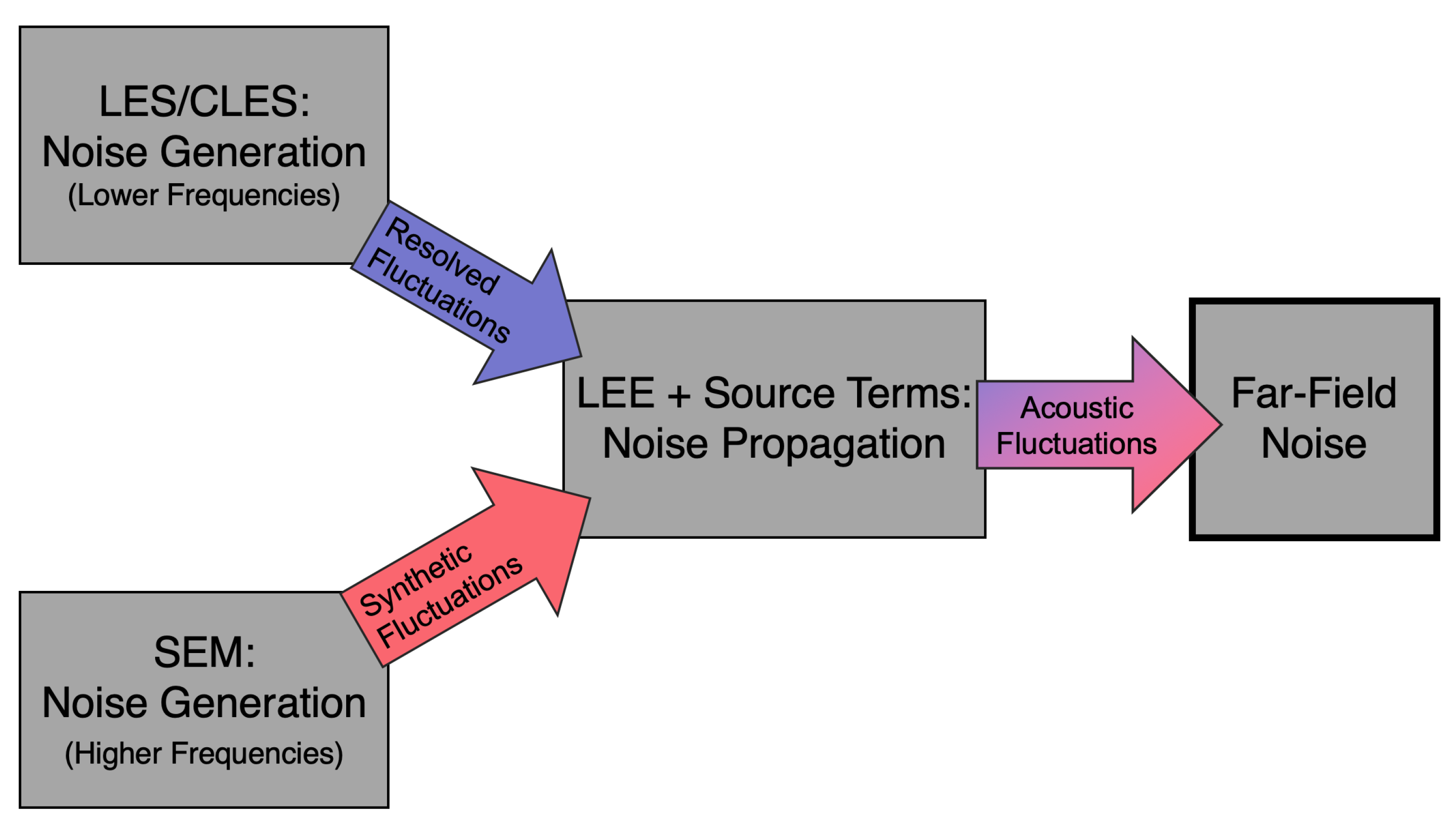
The main idea of
CLST (as shown in
Figure 2) is that resolved and modeled velocity fluctuations are coupled to generate a more complete noise spectrum. The
CLST method combines coarse-grid large-eddy simulations (CLES) and a modified synthetic eddy method (SEM). Using a hybrid CAA method, the jet flow is simulated with the Navier–Stokes (NS) equations in a finite difference multi-block, structured LES solver. Velocity fluctuations produced by the NS LES/CLES solver are passed to the linearized Euler equations (LEE) to generate acoustic sources. The LEE solver then simulates the resulting noise field. The use of LES or CLES turbulence modeling ensures the resolution of large-scale turbulent fluctuations that correspond to low-frequency noise in the far field. Velocities generated by SEM are added to the source terms in the LEE to generate sources corresponding to the missing high-frequency noise.
Figure 2 shows how the proposed
CLST method modifies the CLES/LEE-based noise prediction scheme by adding the generation of synthetic fluctuations to model high-frequency content.
The proposed CLST modeling approach involves the following general steps:
Compute an axisymmetric RANS solution for a jet flow using a or turbulence model to generate a more realistic initial flowfield for the LES simulation.
With the RANS solution as initialization, run the CLES solver until statistically-stationary results are obtained.
Initialize synthetic turbulence from mean RANS flowfield and turbulence information.
Continue the CLES simulation and interpolate CLES fluctuations onto the LEE grid.
Convect synthetic turbulence with CLES velocities, accounting for sweeping and straining of the synthetic velocities.
Compute velocity field produced by the summation of each synthetic eddy.
Combine CLES fluctuations with synthetic fluctuations computed at each time step.
Generate noise sources from LEE source terms and propagate noise with LEE to obtain far-field acoustic pressure data.
As shown in
Figure 2, either LES or CLES (coarse-grid large-eddy simulations) can be used with the
CLST method depending on the desired computational cost. For instance, given the high computational cost of LES, it is unlikely to see industrial application soon. However, if the
CLST method were used with CLES or even Unsteady RANS (URANS) instead of LES, then it might be possible to save significant computational cost due to the lower-fidelity nature of CLES while achieving LES-level frequency resolution. Alternatively, applying the
CLST method to LES, while still expensive, could possibly provide DNS-level frequency resolution at a fraction of the cost of full-resolution DNS.
Two assumptions underpin the
CLST method and aid in limiting the complexity of this problem. The first assumption is that the two-source theory of jet noise holds and that high-frequency noise content is generated by fine-scale turbulence in the shear layer [
10,
15,
17]. In other words, large scales of turbulence correspond to low-frequency noise, and small turbulent scales correspond to high-frequency noise. The second assumption is that a wide range of turbulent scales exists in the jet shear layer, and, consequently, there is a separation between large and small turbulent scales. Furthermore, it is assumed that the small scales are isotropic (per Kolmogorov’s hypothesis) and statistically similar [
44] and can therefore be modeled by a synthetic turbulence method.
Additionally, since the hybrid CAA formulation of the
CLST method only allows coupling from the LES to LEE, the small scales can not influence the large scales and it is assumed that backscatter [
45] should not be explicitly accounted for. However, the influence of the large scales on the small scales, known as sweeping and straining, is assumed to be significant for the radiated noise [
40,
41]. Propagation of acoustic waves is assumed to be a linear, inviscid phenomena even if generated by nonlinear phenomena. Random sweeping occurs when the passing of large energy-containing eddies leads to convection of small inertial-scale eddies [
38,
39,
40,
41]. Local straining is the idea that eddies are stretched and distorted by local fluctuations and accelerations [
42].
It should be noted that the parameters of the CLST method presented here were developed after initial tests for the specific problem under investigation and that the parameters would likely change for different problems. The evolution of these parameters was not considered a topic of interest for this paper. A future sensitivity study could be used to develop more universal parameters. However, the parameters provided here serve as an initial starting point to demonstrate the potential effectiveness of the CLST method.
2.2. Synthetic Eddy Generation
In CLST, small-scale turbulent velocities are synthesized by a superposition of randomized Gaussian eddies, essentially a synthetic eddy method (SEM). An initial RANS simulation with the same flow field parameters as the LES simulation provides turbulent quantities to calculate the eddy amplitude, while the eddy size, orientation, initial position, and “lifetime” are calculated from random values. These randomized values are set on eddy initialization and do not change until an eddy is re-initialized after getting recycled. It should be noted that the values of CLST parameters in this work were chosen in part from preliminary analysis on this specific problem and further study is needed to generalize this method for different analysis conditions.
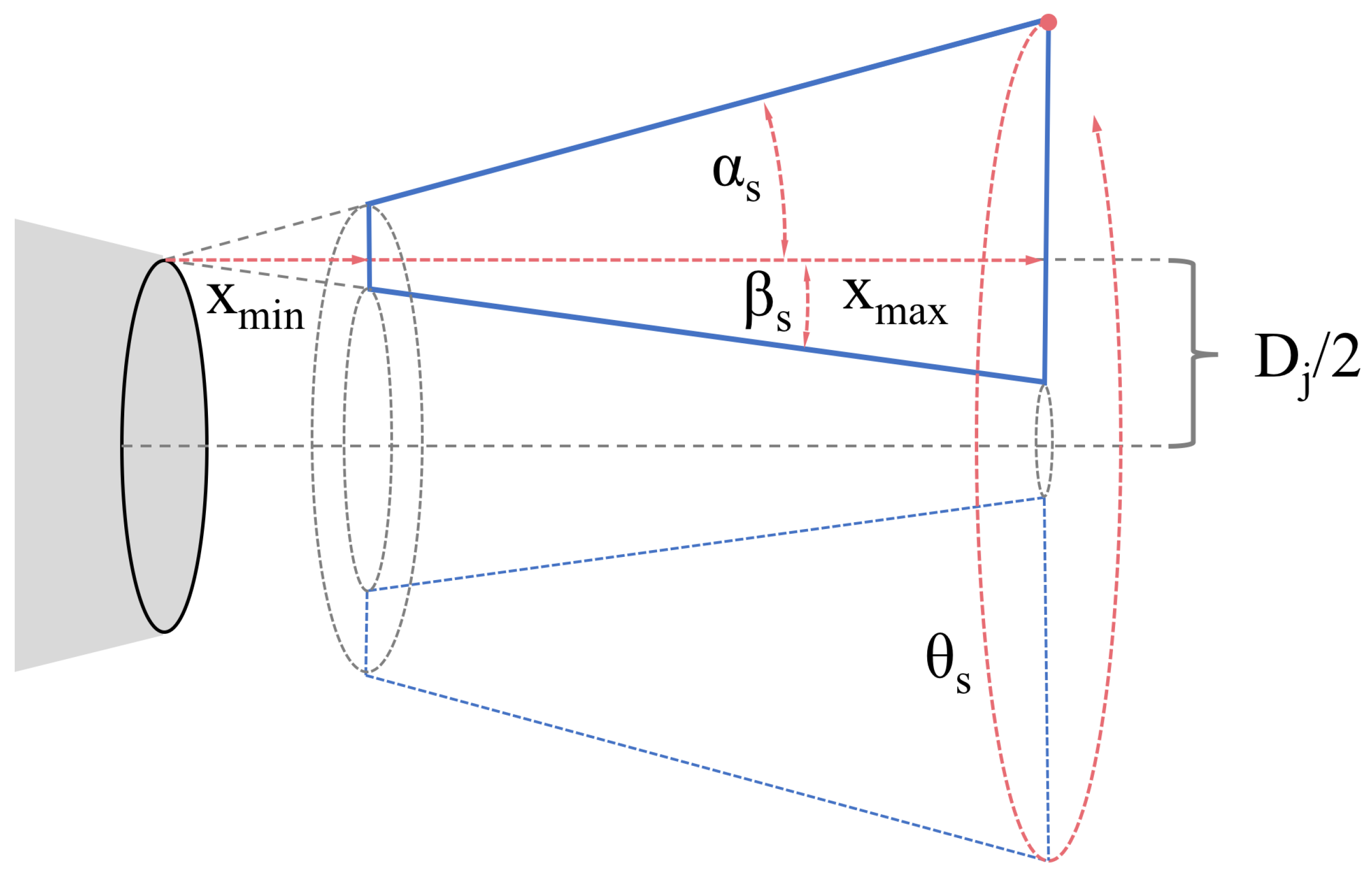
For eddy placement, a source region (the solid lines in
Figure 3) is formed around the jet shear layer, centered on
, where D
j is the jet diameter. The source region is comprised of a cone, with
and
,
and
for this work. The parameters of the cone shape were chosen to mimic the initial shear layer and TKE contours from the LES-only flow field. Eddies are randomly placed in the three-dimensional source region by first choosing a random
value from
to
. Given an
,
and
are chosen from inside the source region.
Synthetic eddies are generated using the following Gaussian shape function:
where the initial eddy center is located at
at the time
, the eddy size is given by
, the eddy life time is given by
, the time ramp width is given by
, the eddy convection velocity is given by
, and the current eddy position and time are given by
and
t.
For
N eddies, the following equations randomize the
nth eddy’s size and orientation for the synthetic velocity fluctuations
:
where
a,
b, and
c are randomized values between −2 and 2 to satisfy the divergence-free condition for a constant convection velocity. For reference, Hirai et al. used both
N = 10,000 and
N = 50,000 eddies, finding that more eddies improved the noise predictions [
32].
The fluctuations generated by all eddies are summed in a point-wise manner to form the synthetic velocity field. At a point
and time
t, the synthetic velocity fluctuations,
, generated by all
N eddies is given by
where
To minimize the computational cost incurred by performing calculating for thousands of eddies across the entire computational domain, the eddy calculation is omitted for any point further than a given distance from the eddy (Equation (
9)), forming a calculation “window”. The convection velocity is included in the distance calculation so that the calculation “window” follows the eddy downstream. Jarrin et al. [
35] employ a similar cut-off in their SEM formulation. A value of
= 2.0 was observed to give good performance while not cutting off eddies stretched by sweeping.
2.3. Eddy Size Distribution
In realistic turbulent jet flows, small eddies are more numerous than large eddies. To mimic this behavior, the synthetic eddies are assigned to a “generation” or bin based on size. Three bins are chosen and distributed in the percentages shown in
Table 1. Due to the Gaussian eddy shape, the actual eddy diameter is approxmiately
, where
is the eddy size. For the rest of this work, eddy size will refer to
, not the actual eddy diameter.
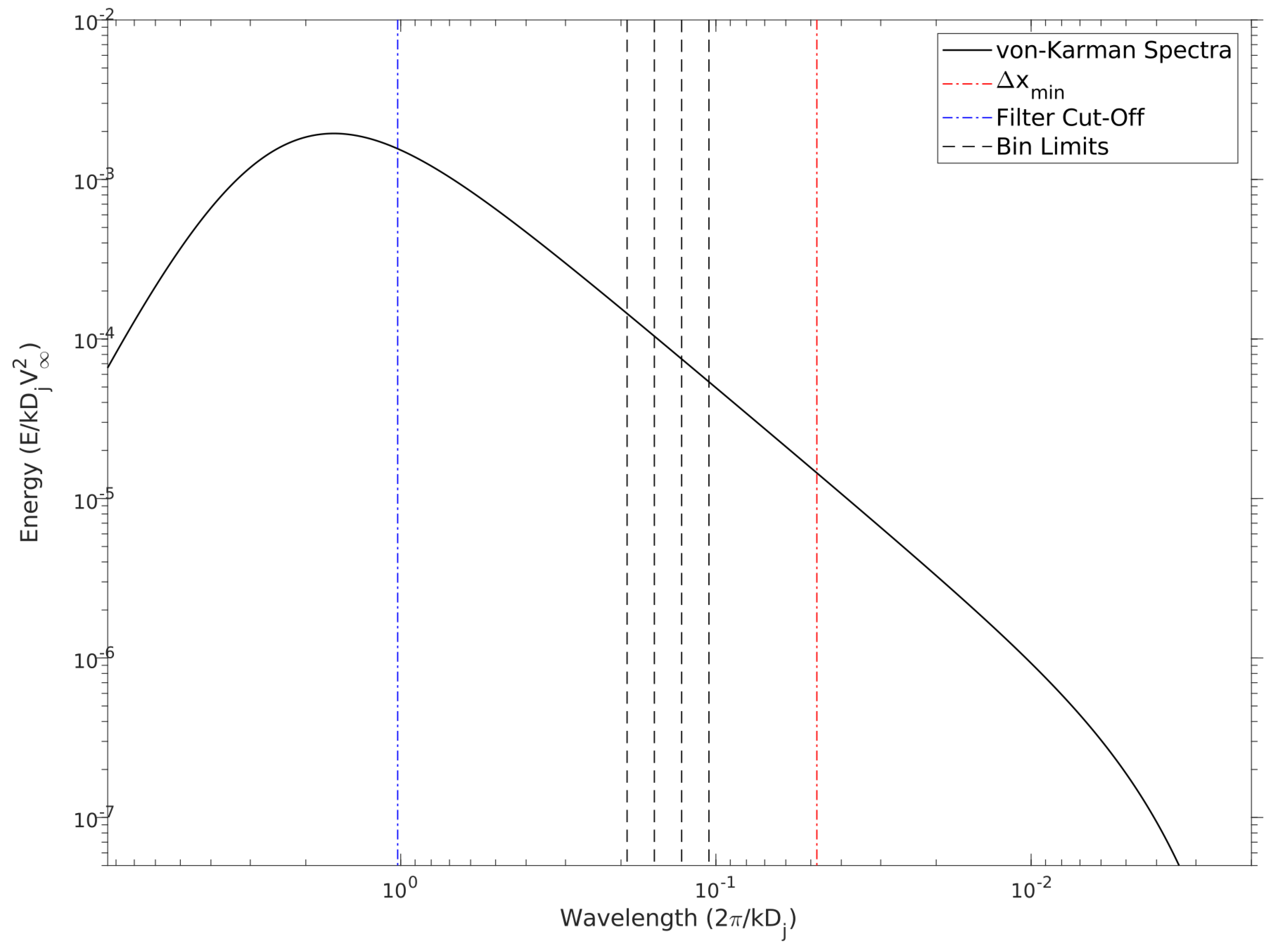
Given that the grid spacing is fine near the jet inlet and coarser downstream, an average minimum grid spacing,
, is calculated across the grid blocks in the eddy source region. The smallest eddy size is taken from the minimum average global grid spacing,
, which is assumed to be the minimum eddy size that the grid can support practically. The largest eddy size,
, is taken from the wavelength corresponding to the filter cut-off,
(as is discussed in following sections, filtering is used to produce a CLES field for
CLST). Wavelengths smaller than the filter cut-off wavelength are attenuated. The factor
is a ratio of the minimum number of points required to resolve the smallest wavelength by the currently-employed DRP scheme to the points per wavelength required in Kennedy and Carpenter [
46]. To further control the eddy sizes, the maximum eddy size was adjusted for this work such that
. These parameters ensure that the smallest eddies are discretized by approximately four grid points on average.
The eddy bins are divided into equal ratios for each bin, with
. The bin ratio,
, is the size increase from one bin to the next. For this work,
is 1.145 based on the grid spacing and filter size.
Table 1 shows the limits for each bin. The von-Karman turbulent kinetic energy spectra is plotted in
Figure 4 for a representative point in the shear layer of a Mach 0.9 turbulent jet. The eddy size related to the fourth-order filter cut-off corresponds approximately to the most energetic large eddies, which is ideal for approximating CLES in the
CLST framework. The distribution of eddies ensures that they reside within the range for isentropic turbulence and do not model the most energetic large eddies. The size of the synthetic eddies does not approach the dissipation range, but smaller eddies could be resolved by using a finer-spaced computational grid.
The eddy size is randomly chosen uniformly over the limits of the bin. Upon re-initialization, the eddies stay in their assigned bin, but the size can change within the limits of the bin. This ensures that the desired size distribution is maintained but allows for randomness in eddy sizes.
2.4. Amplitude Calculation
The amplitude for the
nth eddy is calculated from the von Kármán–Pao energy spectrum for isotropic turbulence following the SNGR method of Bailly and Juvé [
33]. For a given eddy size,
, the wavenumber associated with the
nth eddy is from
. The energy associated with that wavenumber is given by the von Kármán–Pao energy spectrum as:
where
In these equations,
was taken as a constant and
was calculated from the RANS-generated TKE (
) so that the amplitude of the synthetic eddies is only dependent upon the TKE. The wavelength of maximum energy,
, is estimated from turbulent jet data in Pokora and McGuirk [
47].
Finally, for the
nth eddy,
where
is an amplification factor adjusted to produce fluctuations at the desired magnitude. The factor of
is taken from Jarrin et al. [
34] and adjusts the amplitude based on the number of eddies. A value of
was used for the present simulations, although the value of this constant must be investigated in future work.
2.5. Eddy Convection
In the simplest SEM approach, eddy properties such as amplitude and size are fixed at initialization of the eddy, and each eddy is convected with a constant velocity or with the mean RANS flow velocity at the eddy center. These methods of convection do not allow for any distortion to the eddy shape that would occur via sweeping and straining.
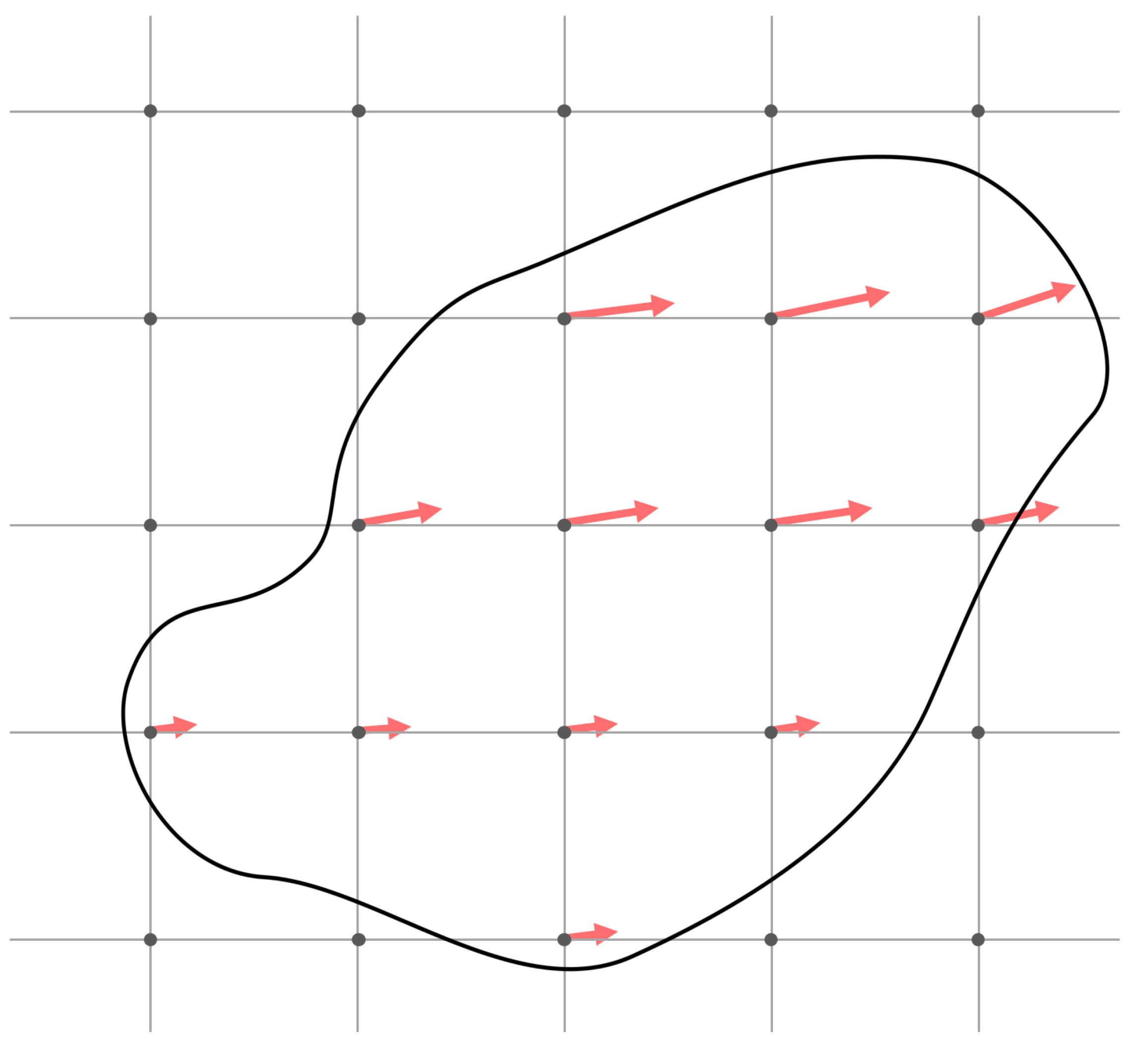
Explicitly tracking and convecting an eddy with a distorted shape is not a straight-forward task in a parallelized, multi-block grid approach if the convection velocity is non-constant due to sweeping by large eddies. To solve this difficulty, the eddy convection velocities in
CLST are taken from each discrete point across the eddy.
Figure 5 shows the pointwise velocity distribution for an eddy distorted by the presence of a non-uniform background flow. Convecting eddies in this pointwise manner saves complexity and computational time by avoiding the point searching and interpolation that would be needed to explicitly track an eddy, and, most importantly, accounts for the influence of sweeping and straining on the synthetic eddies.
To this point, an important feature of the CLST method is that sweeping and straining of the synthetic eddies are modeled. Sweeping occurs when the small-scale synthetic eddies are influenced by the movement and rotation of large-scale eddies. Straining is produced by non-uniformities in the local flow field due to large eddies. To accomplish this in the CLST method, eddies are convected via the instantaneous CLES velocities rather than the mean flow velocities. In other words, the synthetic eddies are convected by the mean jet flow plus any fluctuations resulting from large-scale eddies.
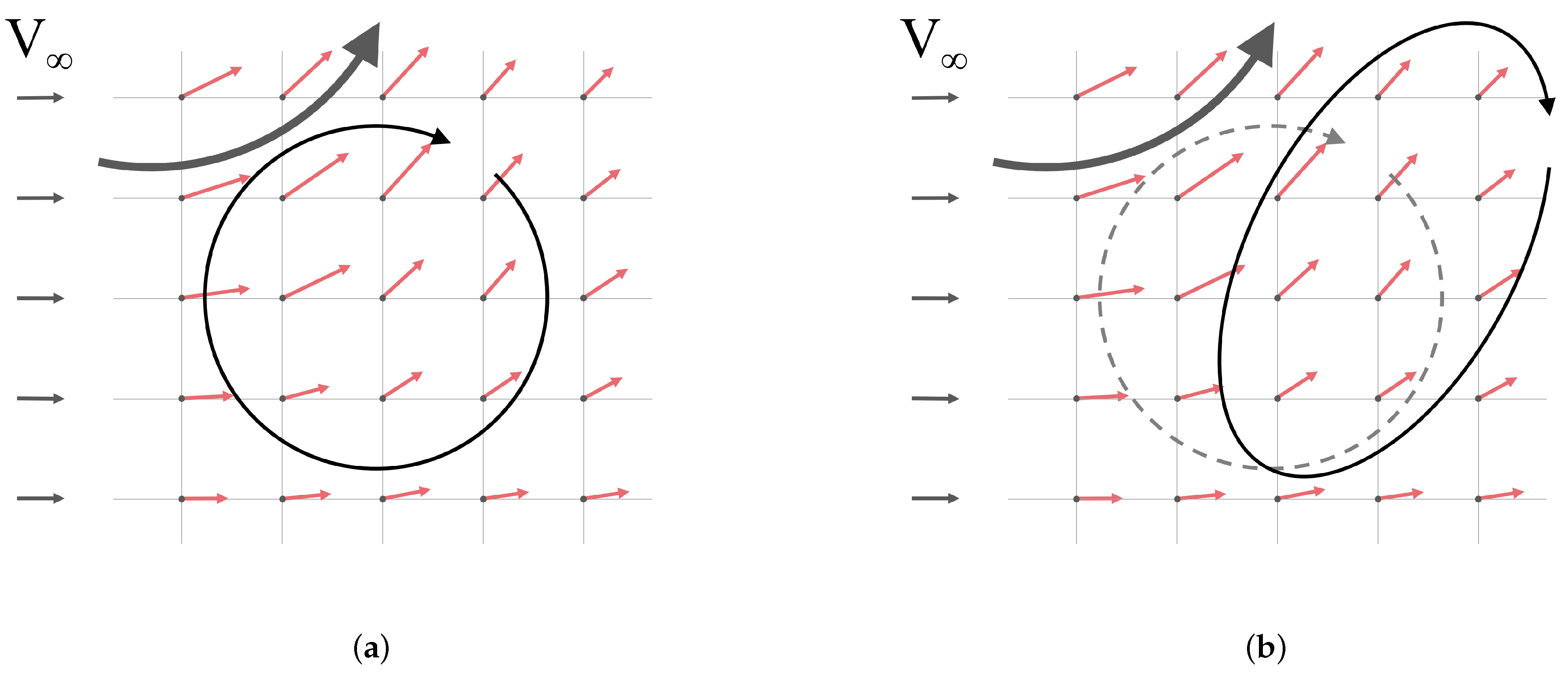
A representative diagram of sweeping due to pointwise convection and is given in
Figure 6.
Figure 6a shows the initial position of a small representative eddy in a flow field influenced by the rotation of a larger eddy. After applying pointwise convection to the eddy, displacement and distortion of the eddy shape due to sweeping and straining can be observed in
Figure 6b.
Pointwise convection leads to changes in certain eddy properties. As a given eddy is convected downstream, the eddy size remains constant, but the eddy amplitude and convection velocity can vary with spatial position. The initial Gaussian eddy shape can also change due to shear, sweeping, or straining effects. Each synthetic eddy is small in size compared to spatial changes in the mean flow field. The lifetime of each eddy is also small compared to the overall temporal fluctuations of the jet. Therefore, it is assumed that changes in the eddy properties over the eddy shape are small, as well as changes in eddy properties over the eddy lifetime since and eddy does not convect very far downstream. Any errors due to violating the divergent-free condition are expected to be minimal to the overall noise produced by the jet.
2.6. Recycling Eddies
At the beginning of the simulation,
N eddies are created and inserted into the flow. They are initialized with an eddy lifetime based on the eddy size, such that small eddies exist for a short time. As the simulation progresses, the amplitude of each eddy is modulated in time with a Gaussian function (see Equation (
1)) so that the eddy fades in on initialization and fades out as it reaches the end of its lifetime. At the end of its life, the eddy is recycled, meaning that the eddy is re-initialized with a new random size, orientation, lifetime, and position in the jet shear layer. The equations for eddy lifetime,
, and the time ramp width,
, were chosen to match the visually-observed time-development behavior of large-eddy structures in LES. Initially, eddies are inserted over a time range of 10-fold the lifetime of the maximum eddy size. Staggering the eddy insertion in this manner prevents similarly-sized eddies from syncing in time, which eliminates global pulsing behavior that can occur if thousands of eddies are recycled simultaneously.
2.7. Coupling of LES and SEM Velocity Fluctuations
In the calculation of the synthetic eddy field, at each point, the contribution from each synthetic eddy is summed at a given point. Once the total contribution of each synthetic eddy is computed, the synthetic velocity fluctuations are added to resolved LES fluctuations and passed to the LEE source terms to generate acoustic sources.
2.8. Numerical Methods
The Navier–Stokes (NS) equations are used for LES and the linearized Euler equations (LEE) are used for acoustic propagation. The three-dimensional Navier–Stokes equations are solved in a conservative form cast in curvilinear coordinates with a multi-block solver. The governing equations and flow variables are non-dimensionalized by the mean flow density , speed of sound , and reference length Dj. Both NS and LEE solvers use the same spatial and temporal discretization algorithms.
2.9. Source Terms for LEE
The LEE equations in primitive variable form are taken from Hirai et al. [
32]. In this formulation, the mean shear terms and mean flow gradients are set to zero to damp instabilities resulting from unbounded homogeneous solutions to the original LEE [
48]. The source terms are the same as Bogey et al. [
48]:
where
The fluctuating velocities
and
in Equation (
14) come from the combined LES and synthetic turbulent fluctuations from
CLST,
. The calibration parameter
is used to adjust the intensity of the sources [
49]. From initial testing, a value of
= 1.3125 was chosen (it is taken as 1.0 by Lafitte et al. [
49]) so that the amplitude of the LEE velocity fluctuations would match the amplitude of the LES velocity fluctuations. The mean density (
) is used rather than the instantaneous density (
) in Equation (
14) because the multiplication of the three fluctuating quantities
is negligible. The bar signifies a time-averaged quantity. The time average of the source terms is not zero, necessitating the subtraction of the mean of the source term [
48].
2.10. Discretization Schemes
The spatial derivatives are discretized using the seven-point, fourth-order dispersion-relation-preserving schemes of Tam and Webb [
50], which are designed to ensure that the schemes calculate the correct wave speeds and propagation characteristics (nondispersive, nondissipative, isotropic) for the main wave modes (acoustic, vorticity, and entropy) [
50], trying to achieve the same dispersion relations as the original partial differential equations. The DRP schemes are simply optimized, explicit finite-difference schemes and are commonly used for LES-based jet noise simulations [
51].
High-order, low-pass implicit spatial filters from Kennedy and Carpenter are used to damp spurious, non-physical waves present in the LES solver [
46]. Explicit filters require less computational effort and are conceptually simpler than implicit filters. The high-order spatial filtering serves a second purpose as an implicit subgrid-scale (SGS) turbulence model for the LES code. Such implicit LES approaches are common in LES-based jet noise predictions [
19,
51]. The tenth-order filter applied to the Navier–Stokes variables produces the best LES results in the present code by suppressing spurious content and providing dissipation for subgrid stresses. Alternatively, using the fourth-order filter effectively produces a CLES flowfield by damping additional small-scale fluctuations.
The time integration is performed using an explicit second-order Adams–Bashforth method (Butcher [
52]).
2.11. Filtering for CLES
In order to evaluate the effectiveness of synthetic velocities supplementing the jet noise spectra via the CLST method, the “missing” LES frequency content must first be measured or estimated. The simplest approach is to artificially generate an under-resolved CLES flowfield by removing resolved fluctuations from a LES simulation in a controlled manner. Applying a low-pass filter to the NS flowfield produces an approximate CLES flowfield by damping the turbulent structures smaller than a cut-off wavelength specified by the filter. Since the effects of the filter are known, the removed fluctuations are quantifiable and can be considered the “missing” noise produced by CLES on an effectively “coarse” grid resolution. A comparison of the acoustic spectra generated by LES (unfiltered) and CLES (filtered) results reveals the missing noise. Filtering thus provides a method to measure the “unresolved” noise and directly investigate the effects of adding synthetic velocities.
As stated previously, the fourth-order filter from Kennedy and Carpenter [
46] can be used instead of the tenth-order filter to produce a CLES flowfield. The version of the fourth-order filter used in this investigation widens the stencil by a point in each direction to increase the filter’s effectiveness. The filter cut-off frequency is estimated using
, where
is the cut-off wavelength assuming the cut-off occurs at 80% of the maximum wave amplitude (
from
Figure 6 in Kennedy and Carpenter [
46]) and
is the maximum resolvable wave number of
. The exact manner in which the filtering is applied to produce CLES results in this investigation is noted in
Section 3.3.
3. Results
Given that the goal of the
CLST method is to account for the effects of fine-scale turbulence, the method was tested at a moderately high Reynolds number with a wide range of turbulent scales present in the jet. A round, isothermal jet was simulated at M = 0.9 and Re = 100,000. These parameters were chosen to match an LES study from Bogey and Marsden [
53] that presented well-resolved results of both the jet flow physics and near-field jet noise spectra (including high-frequency content up to St = 5). Comparisons are made with results from Bogey and Marsden [
53] and Bogey [
19] to investigate the mean jet flow properties and the associated near-field radiated noise predicted by the current LES-LEE method. Finally, the
CLST method is applied to the same jet case.
3.1. Simulation Setup
For purely comparative purposes, the CLES, SEM, and LEE flowfields are calculated on the same computational grid. This also eliminates errors or increased costs due to interpolation between the solutions. Validation for the LEE solver was previously performed both in 2D and 3D, with results (not included here for brevity) showing that the LEE solver predicts the correct acoustic wave propagation behavior [
22].
The computational grid for the jet simulations has 148 blocks and 4.88 million grid points. The domain extends from x = −15D
j to x = 60D
j and out to 40D
j in the y- and z-directions at the widest point. Rather than resolve the interior flow of a nozzle, the jet is modeled as a hyperbolic tangent velocity profile (0.05D
j thick) where the “exit” of the jet nozzle corresponds to the grid’s inlet plane. It is acknowledged that neglecting a nozzle geometry will have an influence on the development of the shear layer, jet flow field, and thus on the radiated jet noise [
2,
20,
54]. However, in the context of developing the
CLST method, the use of an inflow boundary condition is seen as an initial step. Divergence-free fluctuations are forced at the inlet plane to promote the natural transition of the shear layer from quasi-laminar to turbulent [
55]. The number of azimuthal vortex ring modes imposed in the present study is 15 (as suggested [
55]) with an amplitude of 0.06. All other boundaries in the simulation domain employ far-field boundary conditions that use extrapolation. A combination of grid stretching and sponge layers are used at the far-field boundaries to dissipate and filter out fluctuations before they generate spurious acoustic reflections at the boundaries.
Pressure probes were placed in the near-field at the points listed in
Table 2. The probes are divided into two categories. The first set is represented by four probes (P1–P4) equally spaced along the line y = 5D
j, which is close to the jet but far enough from the shear layer to avoid contamination of the acoustic data with hydrodynamic fluctuations. These points should give a good survey of observer locations where high-frequency noise contributes to the spectra. The second set is represented by two probes (P5 and P6) along the line y = 7.5D
j, which are use in a following section to validate the simulation with noise data from Bogey and Marsden [
53]. Frequencies up to St = 5 were observed to be the highest frequencies resolvable on this computational grid at probe locations P1 to P4 [
22] and St = 2 were the resolution limit for probes P5 and P6.
3.2. Les Comparison
Data from Bogey and Marsden [
53] and Bogey [
19] are used to evaluate the accuracy of the present LES simulations for the Re = 100,000, Mach 0.9 jet. Bogey and Marsden [
53] investigate the effect of different grid resolution parameters on the jet flow and noise spectra. Their results are quite detailed, using computational grids with up to one billion grid points and modeling the jet noise out to 75D
j from the nozzle. Additionally, Bogey and Marsden simulate the jet flow with a pipe nozzle geometry. Bogey [
19] presents additional results from identical simulations.
In comparison, the grid of the present simulation does not extend to the far field with adequate resolution to resolve pressure fluctuations past 15Dj and has at least 50-fold fewer grid points (4.8 million vs. 250 million). The present simulation method employs an inlet plane for the jet rather than a physical nozzle geometry. Disturbances are imposed at the inlet to excite the jet turbulence. Only the near-field region of the computational grid for has sufficient resolution to capture noise data. Given the high level of resolution in Bogey and Marsden’s results and the computational limitations of the present simulations, identical replication of Bogey and Marsden’s results is not expected. However, if the same mean jet flow and turbulence properties are captured by the present simulation, the noise spectra should agree well for low and mid frequencies.
It is expected that Bogey and Marsden’s use of a nozzle geometry leads to differences when comparing the present simulations. In the present LES, disturbances are imposed at the inlet to stimulate fluctuations at the inlet and produce a turbulent jet. The data from the present simulation are most similar to results from Bogey and Marsden for an initially laminar, transitioning jet. Given that a nozzle geometry is not included in the present simulation and that some small region of transition is expected when imposing a jet flow at an inlet plane, a comparison to an initially laminar jet is acceptable.
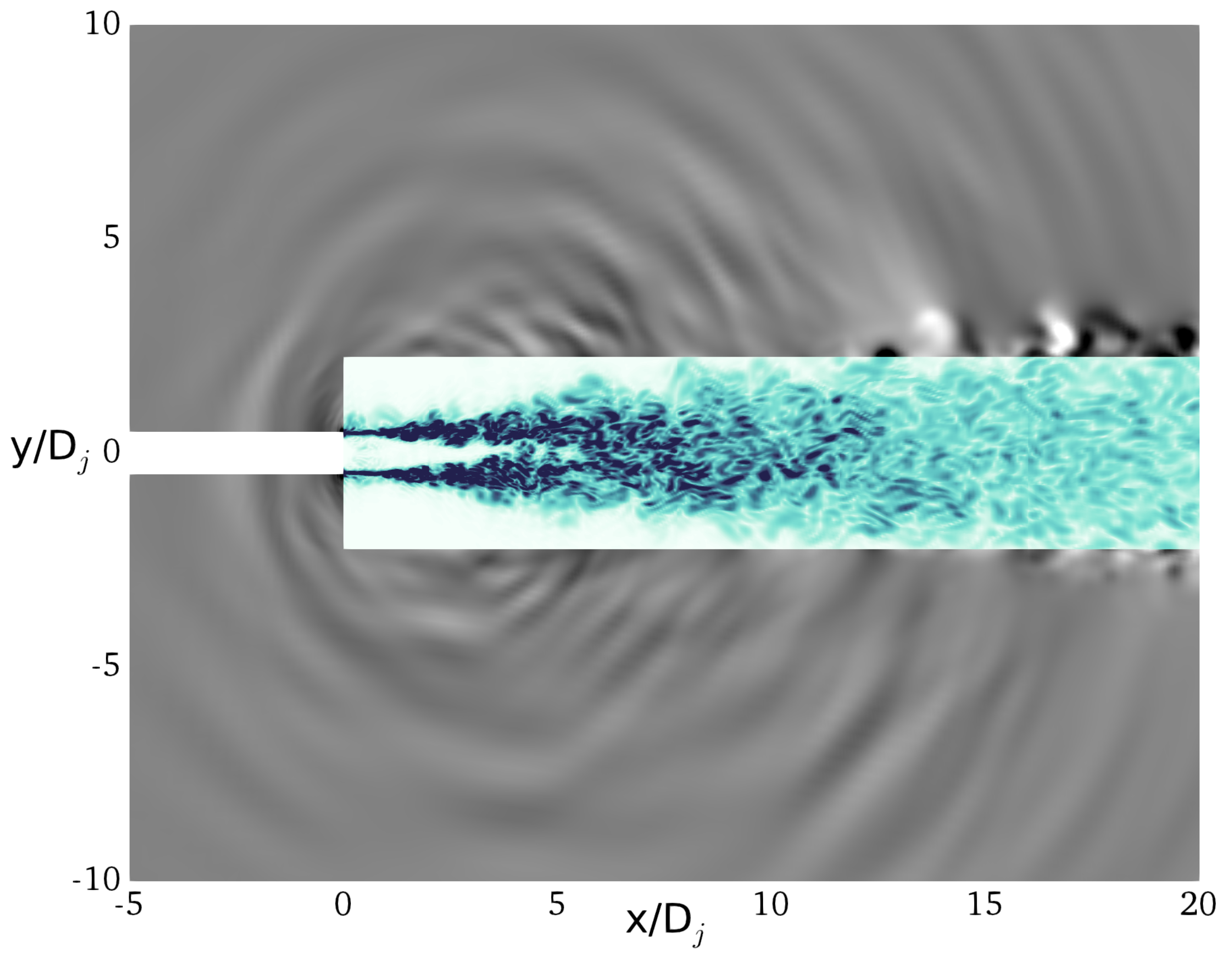
Combined contours of instantaneous vorticity and acoustic pressure provide an initial qualitative investigation of the results from the present simulation.
Figure 7 is plotted in a style similar to results from Bogey and Marsden [
53], with vorticity contours in the center (over the range y =
) surrounded by the near-field pressure fluctuations. Vorticity is scaled by
and pressure is presented in Pascals. The potential core ends around 5D
j. Both large- and small-scale turbulent motions are observed prior to the merging of the shear layers. As the grid for the present simulation coarsens near x = 15D
j, the turbulence dies off sooner than in Bogey and Marsden’s results.
In
Figure 7, pressure waves with strong amplitudes are observed radiating downstream at approximately a 30
angle measured from the jet axis. These waves are related to the noise from the large-scale coherent structures [
53]. Additionally, small-scale pressure waves are seen radiating from the shear layer before x = 5D
j. These two phenomena are the expected essential components of jet noise. The fine-resolution results of Bogey and Marsden show many small-scale pressure fluctuations. Although small waves are observed in the present simulation, they are not well resolved by the present computational grid.
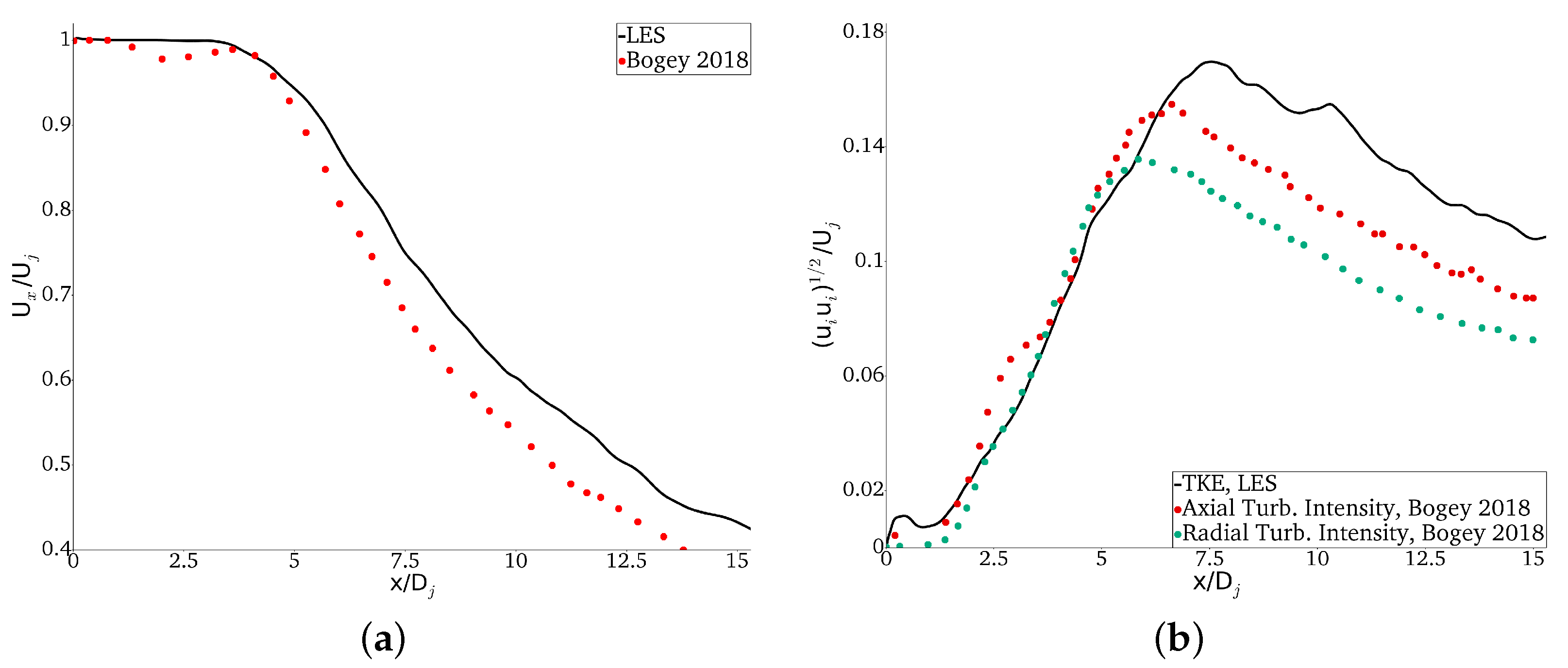
For a more quantitative comparison, centerline flow properties are compared to replicated data (data reproduced with permission from author) from Bogey [
19]. Mean axial velocity is plotted in
Figure 8a. The velocity decay matches Bogey’s data well, and the decrease in velocity around x = 4.5D
j −5D
j indicates the end of the potential core. More rapid turbulent development in this jet leads to a shorter potential core than is typically expected (around x = 7D
j [
53]), but the present simulation shows a slightly longer potential core than Bogey’s data. The intensity of roll-up and pairing of vortical structures in the transitioning shear layer causes the jet to develop more rapidly, shortening the potential core.
Root mean square values of axial and radial turbulence intensity from Bogey are plotted in
Figure 8b. The square root of time-averaged TKE from the present simulation is plotted for comparison. Although the quantities are not identical, they are similarly derived from multiplications of the turbulent velocity fluctuations and demonstrate that the present simulation predicts a similar turbulence decay rate along the centerline. The rise in turbulence indicates the merging of the shear layers at the end of the potential core. The present simulation shows a slightly elongated potential core compared to Bogey’s data. Both centerline velocity and turbulence intensity results demonstrate that the mean flow properties in the present simulation agree well with LES results from Bogey.
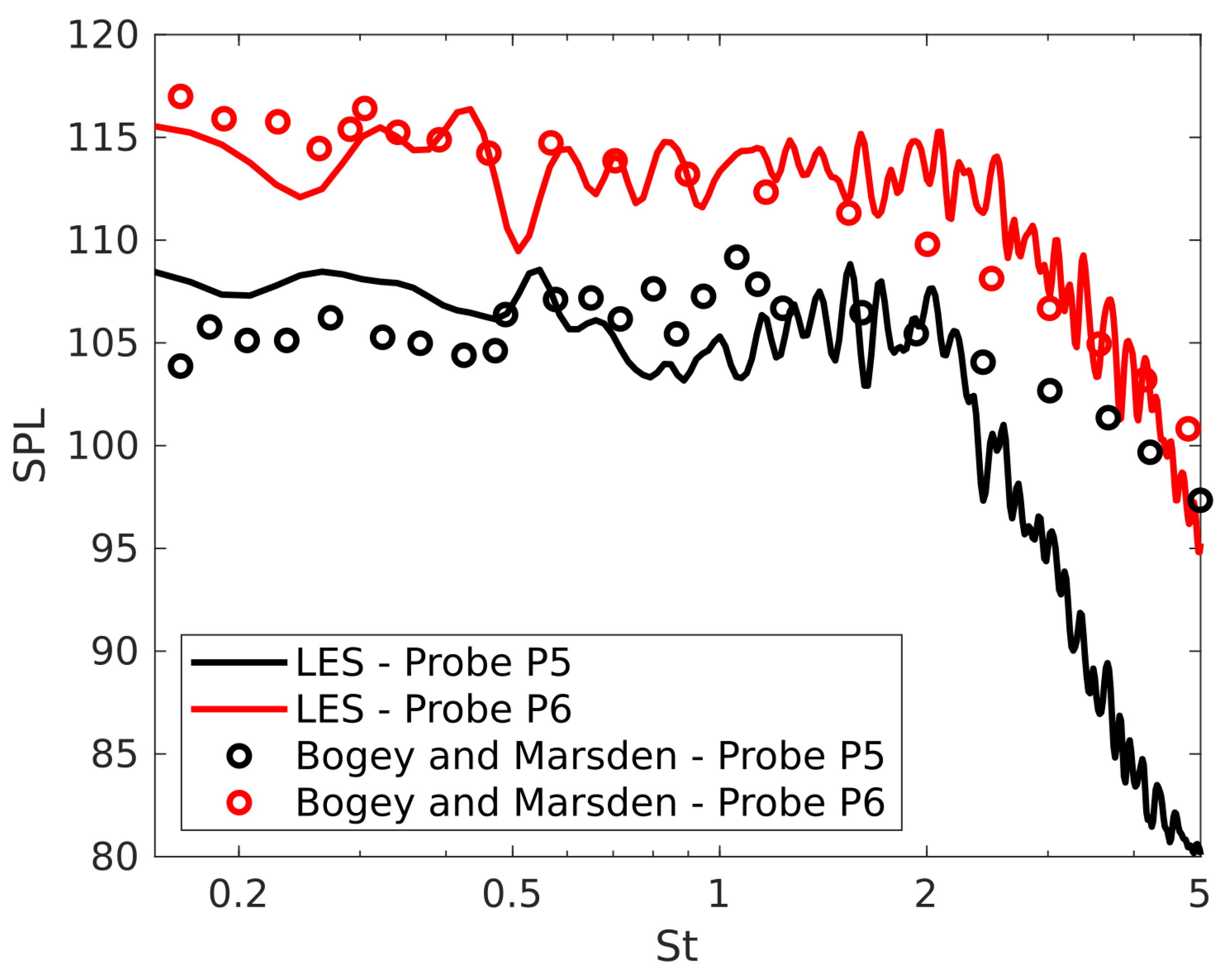
Two probe locations in the near-field of the jet along the line y = 7.5D
j are used for comparison of the noise spectra from a time-history of pressure: point P5 (x = 0D
j) and Point P6 (x = 10D
j), shown in
Table 2.
Figure 9 shows SPL spectra for the two points from the present simulation and also from Bogey and Marsden [
53]. The pressure from the present simulation is taken from the Navier–Stokes solver, since the probe locations are still in the near-field of the jet where the grid resolution is fine enough to capture noise data. For both probe locations, the frequency spectra from St = 0.2 to St = 2 are matched. Higher-frequency roll-off is observed above this frequency, and it is more pronounced in Probe P5, with an under-prediction of 20 dB at St = 5. The drastic roll-off in high-frequency content for probe P5 is due to coarser grid resolution near this probe location. The frequency decay is less obvious for probe P6, where grid resolution is finer. The noise at probe P6 under-predicts Bogey and Marsden’s data by approximately 5 dB at St = 5. The high-frequency roll-off is expected because fewer points were used in this computational grid compared to Bogey and Marsden’s grid.
With this favorable spectral comparison, it is expected that this grid and case setup can reliably resolve the jet spectra up to at least St = 2 at these probe locations, or up to St = 5 in locations where the grid spacing is finer. A perfect comparison with Bogey and Marsden’s data is not expected, given the differences in grid resolution and simulation technique. However, these results demonstrate enough quantitative and qualitative similarities to assume that the correct jet physics and noise mechanisms are captured by this computational setup.
3.3. CLST Noise Spectra
The primary goal of CLST is to supplement the high-frequency content of LES. First, the noise spectra is analyzed, followed by an investigation of the turbulent properties of CLST in a following section. The same M = 0.9 jet was used to evaluate the CLST method.
Conceptually, CLST works by adding synthesized small-scale fluctuations to under-resolved LES (referred to as CLES here). To properly evaluate the noise generated the the CLST method, three results are needed: LES, CLES, and CLST. The LES-generated noise spectra provides the known, expected target solution for the CLST-based noise results. The CLES-generated noise spectra represents the results of an under-resolved LES simulation, an example of when the CLST method would be useful in predicting a full noise spectra. In a typical application of CLST, the unresolved noise spectra would not be known. However, in this instance, the under-resolved portion of the noise spectra on this grid can be obtained by comparing to the LES-generated noise spectra. The CLST-generated noise spectra represents using the CLST method to model the high frequencies that are not resolved by the CLES noise prediction. The CLST-generated spectra can be compared to the LES-generated spectra to evaluate the characteristics of the high-frequency noise added by the CLST method.
In the following analysis, the data were obtained from one simulation run which gave LES, CLES, and
CLST flow-fields simultaneously. Pressure histories for LES were taken directly from the NS solver because the grid has sufficient resolution in the near-field for noise. Although not shown here for brevity, near-field noise spectra obtained in this manner from the LES solver demonstrated good agreement with the noise obtained from the LEE solver [
22].
Filtering was applied to the LES velocity field to obtain CLES pressure histories and velocities, which can be seen as under-resolved LES on the current computational grid. The jet noise produced by the LES and CLES flowfields was computed using the near-field pressure probes. The spectra from CLES can be considered the noise radiated from an under-resolved LES simulation. Synthetic turbulence was combined with resolved large-scale velocity fluctuations (filtered CLES velocities) into the LEE source terms, giving the noise produced by the CLST method. Pressure histories for CLST are taken from the LEE solver. The frequency content added by the synthetic turbulence was revealed by comparing noise spectra from LES, CLES, and CLST.
This approach is representative of adding synthetic turbulence to an under-resolved LES simulation and recovering the “missing noise”, but in this case, the added noise is quantifiable and comparable to the “missing noise” because the “missing noise” has been removed by a filter with known frequency properties. The excellent agreement that was previously demonstrated [
22] between the NS and LEE pressure makes this is a valid comparison for all three methods.
For the computation, a non-dimensional time-step size of was used, which equates to a CFL of 0.13. This was required for stability of the Adams–Bashforth time-marching algorithm. Obtaining all three results from one simulation is only performed for comparison purposes in this investigation.
In this evaluation of the CLST method, 8000 eddies were inserted into the shear layer. Preliminary results revealed that adding 8000 eddies formed a reasonable balance between increased computational cost and additional high-frequency noise in this simulation. A fourth-order filter was applied to the LES field twice for every time step to obtain the CLES field. The average minimum grid spacing in the source region was = 5.546 . All other CLST parameters can be found in the methods section.
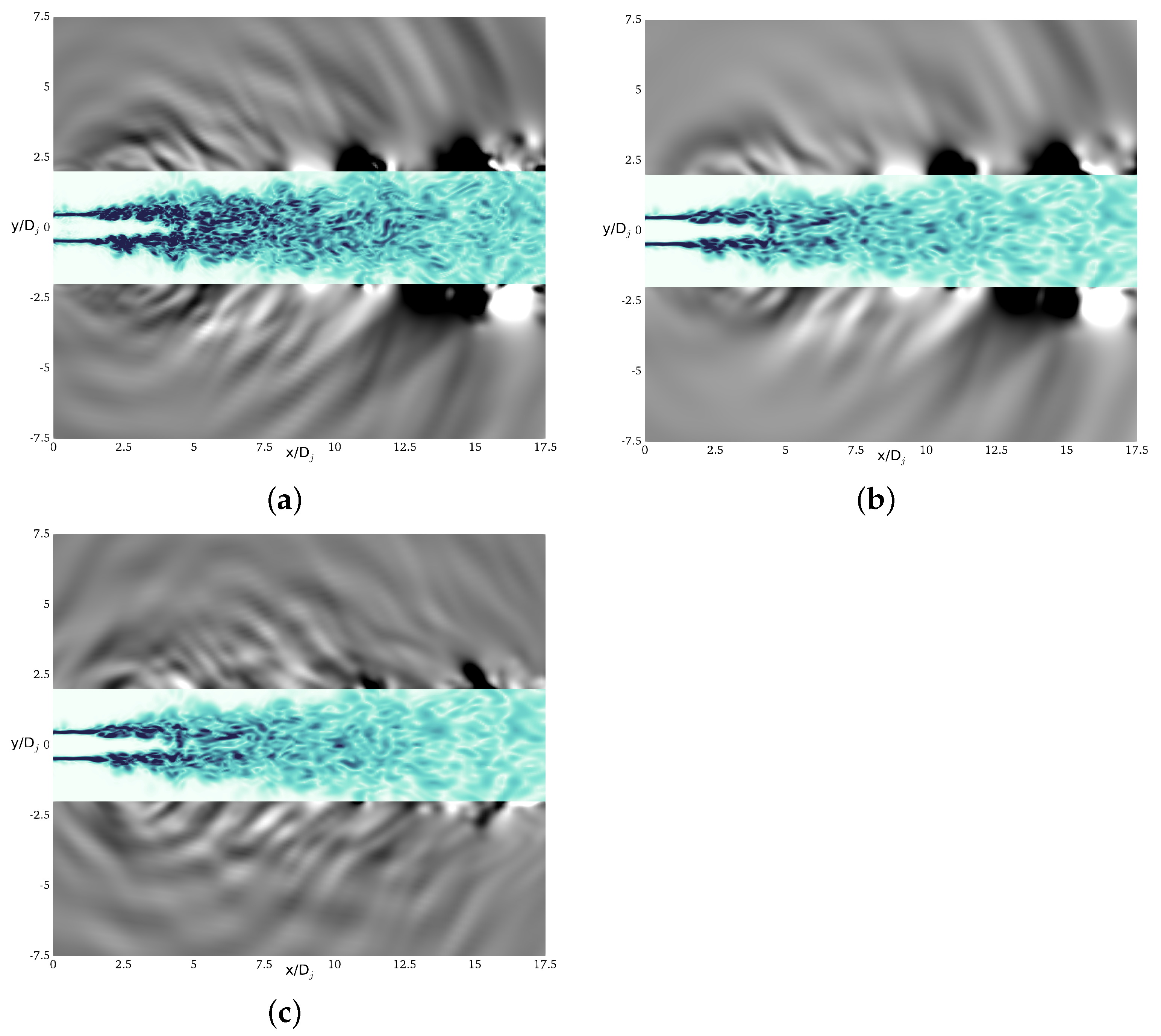
A qualitative comparison of the jet turbulence and near-field pressure spectra are shown in
Figure 10 at the same instance in the simulation. Contours of vorticity (shown as non-dimensional quantities scaled by
) are shown for a range of y =
. Pressure field contours are shown in units of non-dimensional pressure (scaled by
). LES results in
Figure 10a reveal the developing turbulent jet, the merging of the potential core around x = 5D
j, and the slow dissipation of turbulence downstream past 15D
j.
The pressure field displays several expected noise phenomena: large-scale waves radiating at 30
, large-scale pressure fluctuations, and smaller, spherical waves radiating from the early shear layer. The CLES results in
Figure 10b reveal that filtering removes the fine-scale turbulence while leaving large-scale turbulent structures untouched. The large-scale pressure fluctuations are still evident in the CLES pressure field, but damping is observed and small-amplitude pressure fluctuations are not observed, especially upstream of the potential core. In
Figure 10c, with the synthetic turbulence added to the CLES flow field, there is a nearly-negligible increase in the intensity of turbulent velocities within the first 5–7 nozzle diameters. However, additional small-scale pressure waves are discernible in
Figure 10c, indicating that the synthetic eddies from
CLST are generating additional noise. Note the angling of the large-scale pressure waves toward the downstream, indicating the expected directivity of the most significant noise. Slight visualization artifacts are present in the flow field in
Figure 10a,c, but these do not contaminate the pressure spectra.
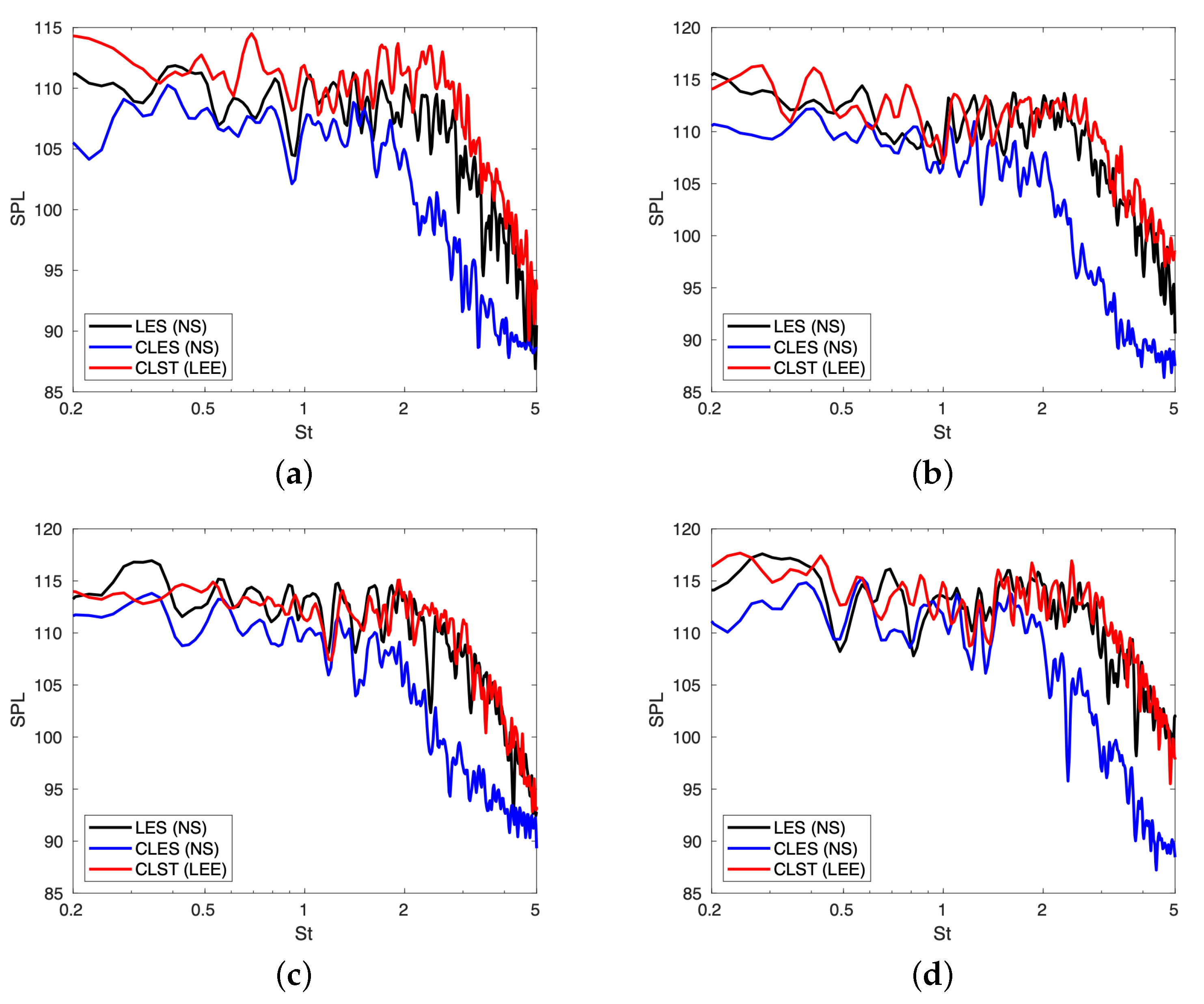
Pressure data was recorded from the
CLST simulation every 15 time-steps over a total of 140,000 iterations. The probe locations are given in
Table 2. The noise spectra from the pressure histories were obtained by a Fast Fourier Transform (FFT). The spectra for probe locations P1 through P4 in
Table 2 are shown in
Figure 11. Spectra from LES, CLES, and
CLST are compared. Frequencies from St = 0.2 to St = 5 are present in the LES noise spectra. The noise produced by CLES filtering shows strong high frequency at roll-off starting at frequencies of St = 1 to St = 2. At St = 2, CLES is around 10 dB below LES for all four points. The CLES filtering also reduces portions of the low-frequency noise spectrum by up to 5 dB in places, potentially indicating that the filter influences a wider range of frequencies than intended. For all four probes, the addition of synthetic turbulence leads to the recovery of the filtered frequencies in the range St = 1 to St = 5. Several small differences (less than 5 dB) are observed between the LES and CLST spectra at various points. Notably, at point P1 (
Figure 11a), there is an over-prediction around St = 2. Overall, at all four locations along the line y = 5D
j, the shape and level of the LES spectra is modeled well with
CLST.
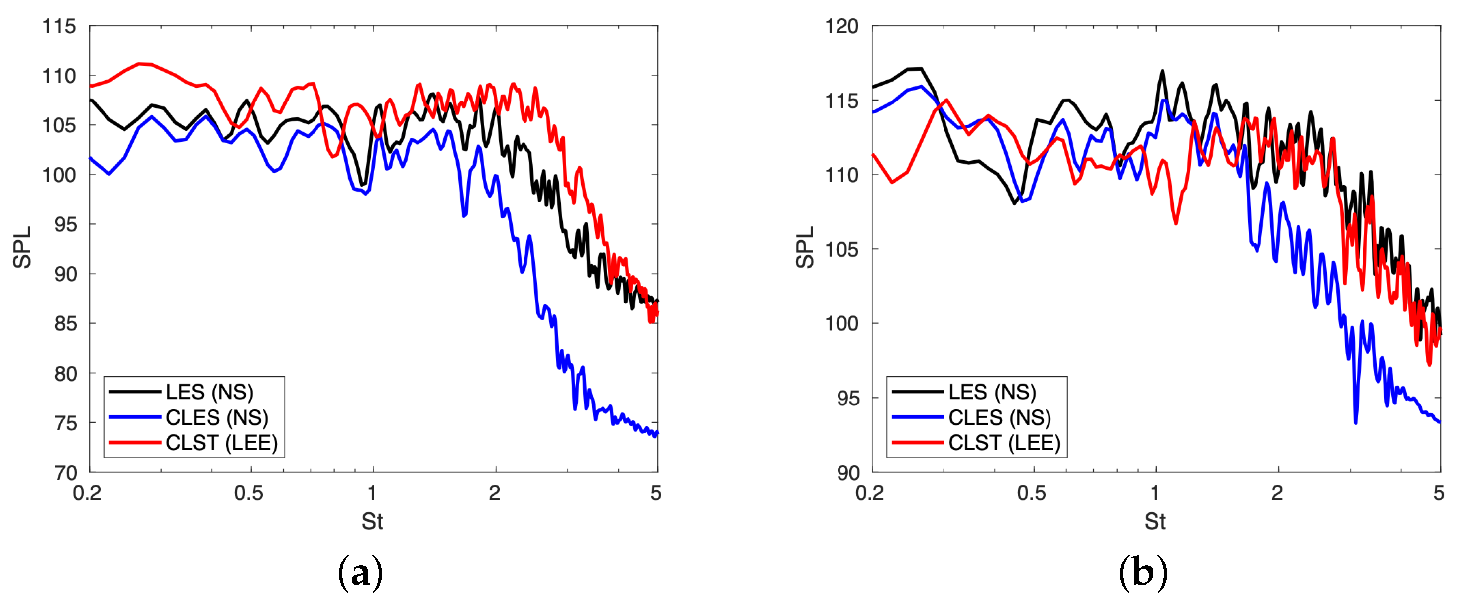
The spectra from points P5 and P6 are shown in
Figure 12. Again, filtering removes frequencies above St = 1. Some evidence of roll-off from grid resolution can be observed above St = 4 for both probe locations. Again, the noise from
CLST recovers the missing spectra and matches LES spectra. Point P5 shows slight over-prediction around St = 2.
In two of the probe locations directly to the sideline of the nozzle, Point P1 (
Figure 11a) and Point P5 (
Figure 12a), an over-prediction of 3–5 dB was observed around St = 2–3. It is possible that excess noise is generated from the synthetic eddies at these frequencies, but the exact cause of these slight differences is unclear.
The intensity of the synthetic eddies was tuned to match the amplitude of the pressure waves, not the LES velocity fluctuations. The synthetic velocities were combined with the CLES velocity fluctuations in post processing, but these results are not presented here because the the synthetic velocities did not make a visibly discernible difference in the CLES velocity field. This is an indication that the synthetic turbulence field generates more noise than expected, which could be the result of inserting unrealistic eddies into the flow. Alternatively, the distortion of eddies due to sweeping and straining could violate the divergence-free condition and generate additional noise.
Ideally, matching the turbulent flow field first would provide an anchor point for further applications of the
CLST method, eliminating the need to re-tune the amplitudes of the synthetic eddies to match the pressure waves for each simulation. It may be difficult to match both turbulent flow properties and the noise spectra. Hirai et al. [
32], who also employed a synthetic turbulence model for jet noise predictions, had a similar issue with over-predicting the noise levels when first tuning their model to match turbulent statistics. However, given that the noise results match well in the previous section and meet the primary goal of the
CLST method, the differences in the turbulent flow field are acceptable for the current stage of
CLST development.
4. Discussion
In the CLST framework, synthetic turbulence is used to supplement an under-resolved jet noise spectra. Even with a moderate number of synthetic eddies, the present simulation results demonstrate the effectiveness of this approach for a high subsonic jet. For all recorded probe locations in the Mach 0.9 jet simulation, the CLST method recovered the high-frequency noise removed by filtering. Despite small differences in the noise spectra, it is clear that CLST can supplement the missing noise spectra from under-resolved turbulence and capture the correct noise spectra curves for near-field observer locations.
Previous applications of synthetic turbulence to jet noise predictions (Fukushima [
31] and Hirai et al. [
32]) demonstrated the effectiveness of synthetic turbulence models (including synthetic eddies) for jet noise predictions. However, both of these approaches use steady RANS simulations to solve for the mean background flow, which means that the influence of convecting, large-scale anisotropic turbulent structures cannot be modeled properly. Hirai et al. [
32] partially account for this with a time decorrelation process that models the influence of the shear from the mean background flow on the synthetic turbulence. This approach is still limited since the background flow is obtained from steady RANS. A more physically-accurate model would include localized, time-varying influences on the synthetic turbulence from the background flow, such as the effect of large-scale convected eddies. Recall that large-scale turbulent structures are significant to jet noise production [
10,
14,
15,
17,
18], and therefore, their influence on the flowfield must be properly accounted for.
The CLST method advances the synthetic turbulence modeling approach by directly simulating the large anisotropic turbulence scales in the mean flow and using their motions to account for sweeping of the synthetic turbulence, including additional key physics in the jet noise modeling. Overall, this introduces a new framework for modeling the missing high-frequency content in jet noise simulations.
The primary drawback of the CLST method is that the eddies appear to generate more noise than anticipated when the intensity of the synthetic turbulent field is matched to the LES turbulence intensity. This led to reducing the amplitude of velocity fluctuations to the point that the combined resolved and synthetic velocity fluctuations from CLST did not approach the levels of resolved velocity fluctuations observed in the LES solution. A major focus of future investigations will therefore be to match the turbulent flow quantities of LES without over-predicting the noise, as well as fine-tuning and generalizing the synthetic eddy parameters. The extra synthetic eddy noise could result from inserting unrealistic synthetic eddies into the flow. Additionally, distortion of the eddies due to sweeping and stretching may violate the divergence-free condition, leading to extra noise.
A second drawback of the
CLST method was that the cost was higher than expected due to a large memory overhead. The extra numerical cost incurred by calculating
CLST with 8000 eddies was approximately 8-fold that of the LES + LEE solvers. With optimization, it is estimated that
CLST would only cost 1.5 or 2-fold more than a baseline LES + LEE solution. It would be desirable to use more eddies (upwards of 50,000 were used by Hirai et al. [
32]), so future work will also focus on a more efficient code optimization to reduce the high-memory cost of the current implementation of
CLST.
It is recognized that significant cost savings could be realized by using a coarser LEE grid since the resolution requirements are lower for LEE than for a scale-resolving NS solution, although for this study all grids were kept the same for simplicity. Even so, the computational cost increase for CLST vs. CLES was moderate in the Mach 0.9 jet simulation. In contrast, halving the grid spacing for a LES + LEE simulation may lead to a 16-fold increase (8x for LES, 8x for LEE) in computing time if the same grid is used for LEE as LES. In this light, the added cost of CLST is still cheaper than simply increasing the grid resolution of the LES solver to achieve a similar noise spectra with high-frequency spectral content.


