A Machine Learning Approach for Global Steering Control Moment Gyroscope Clusters

Abstract

This paper addresses the problem of singularity avoidance for a 4-Control Moment Gyroscope (CMG) pyramid cluster, as used for the attitude control of a satellite using machine learning (ML) techniques. A data-set, generated using a heuristic algorithm, relates the initial gimbal configuration and the desired maneuver—inputs—to a number of null space motions the gimbals have to execute—output. Two ML techniques—Deep Neural Network (DNN) and Random Forest Classifier (RFC)—are utilized to predict the required null motion for trajectories that are not included in the training set. The principal advantage of this approach is the exploitation of global information gathered from the whole maneuver compared to conventional steering laws that consider only some local information, near the current gimbal configuration for optimization and are prone to local extrema. The data-set generation and the predictions of the ML systems can be made offline, so no further calculations are needed on board, providing the possibility to inspect the way the system responds to any commanded maneuver before its execution. The RFC technique demonstrates enhanced accuracy for the test data compared to the DNN, validating that it is possible to correctly predict the null motion even for maneuvers that are not included in the training data.

1. Introduction

Control Moment Gyroscopes (CMGs) are widely used in spacecraft control for maneuvering and they have been successfully employed for a wide range of space missions [1,2,3]. Since they are momentum-exchange actuators, the shape and the size of the momentum envelope depends on their configuration. The size of the envelope is proportional to the maximum available torque that can be generated in a certain direction. From all the possible configurations, the conceptual pyramid configuration is commonly studied in the literature due to the nearly 3-axis symmetric and spherical momentum envelope it produces [4]. Despite the extreme torque magnification property and the rapid response, the singularity problem poses a barrier to make CMGs popular in attitude control [5,6]. In general, singular states are divided in two main categories. If a singular state can be escaped by null motion, it is classified as passable or hyperbolic [7], otherwise, the singularity is referred as elliptic. In both cases, the manipulability index can be used as a performance measure to indicate the approach to singularity, as proposed in [8]. An extensive study in singularities topology has been made in [9,10,11]. Dealing with singular states is commonly classified in two different categories: the singularity avoidance and the singularity escape logics [12]. The steering logics that avoid a singular state without creating torque error, usually being more precise, are included in the first category, whereas the steering logics that induce torque error to escape a singularity, commonly trying to minimize it, belong to the second one. Both approaches make use of some local information in the vicinity of the current gimbal configuration [13,14].

Path planing techniques that take into consideration the whole maneuver are usually focused on choosing the initial gimbal configuration that optimizes the performance of the system during the trajectory [15,16,17]. A global steering path planing approach is discussed in [18,19], where an A* search algorithm is used to steer the gimbals of a CMG cluster in the null space. An enhanced global steering approach is also presented in [20], which does not use a node visit histogram and offers the possibility for near-real time implementation. Such approaches are capable of dealing with singularities before encountering them, but a new optimization problem has to be solved for every maneuver commanded. A path-planning technique that blends the pseudo-spectral and direct-shooting methods upon gimbal saturation and singularity constraints is presented in [21]. Another trajectory-planning approach to reduce the possibility of CMG saturation is described in [22], while a global singularity-avoidance steering law that aims to minimize the time integral of the quadratic sum of the gimbal rates is presented in [23]. Path planning techniques based on energy consumption have also been studied in [24] for double gimbal CMGs.

The advances in computer science and Machine Learning (ML) are establishing a new era for a variety of science fields, even though models of artificial neural networks have been used since about the 1950s [25]. The developed algorithms are employed in pattern recognition, object detection, and numerous aerospace-related applications [26,27,28]. The availability of a great amount of information and data is encouraging the substitution of the heuristic approaches, which are widely used so far, by machine learning techniques. Combining data-sets with the computational efficiency of modern computers, it is possible to create a system able to learn and come into conclusions as well as humans do. However, in the field of CMGs no extended research has been conducted from the perspective of ML. An adaptive control approach using neural networks for spacecraft systems with uncertainty under external disturbances is proposed in [29,30], whilst an estimation of gimbal angles through a similar network is discussed in [31]. Another adaptive neural network is designed in [32] to add robustness with respect to model uncertainties for an under-actuated double gimbal CMG, while a similar network in combination with the dynamic inversion technique is presented in [33] for a variable speed CMG cluster. The use of a recurrent neural network both for moments of inertia estimation and for attitude control without the knowledge of the satellite dynamics is studied in [34]. In [35], a neural network-based fault diagnosis scheme is proposed to address the problem of fault isolation and estimation for CMGs. A Q-learning controller for a 3-CMG cluster is described in [36], which aims to provide attitude control about the yaw axis. A comparison among the Q-learning and a PID controller shows that the Q-learning controller is not only harder to be implemented but also presents a worse performance in terms of stabilization time and overshooting. Besides CMG-related control, an iterative learning control [37] and a robust adaptive control with unknown actuator non-linearity [38] have also been presented.

It is evident that no research has been done in relating the null space motion with the initial gimbal configuration and the desired maneuver through a data-set, even though the redundancy of the system offers such possibilities.

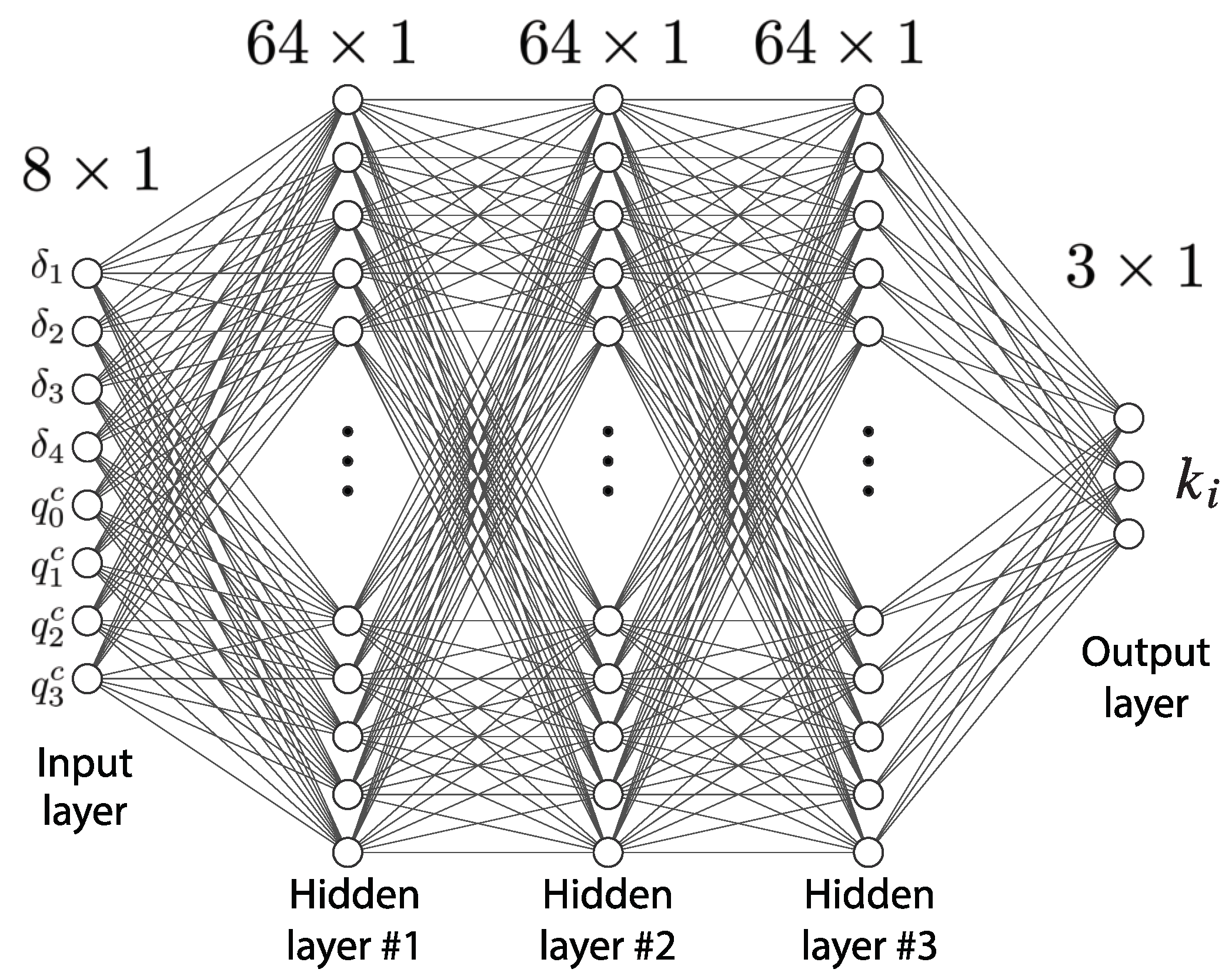
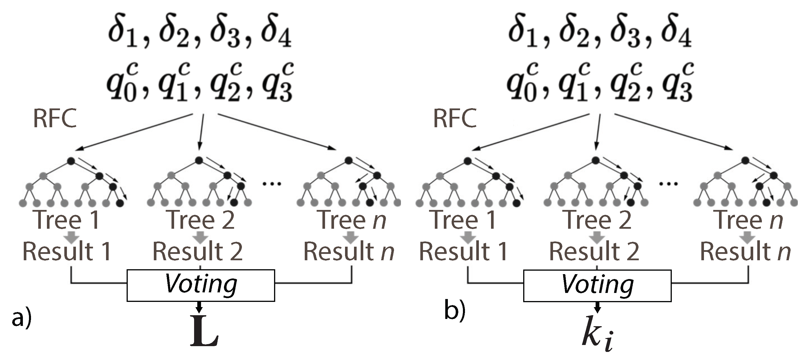
In this paper, a method of improving the performance of a spacecraft employed with CMGs by investigating an optimal path in the gimbals’ null space is presented. It takes into consideration the whole desired/commanded maneuver (global search), in contrast to the most conventional gradient methods that exploit some information only in the region near the low performance configurations. Two different ML techniques—Deep Neural Network (DNN) and Random Forest Classifier (RFC)—are implemented to deal with the global steering problem, without the need of creating and searching a new graph every time a new maneuver has to be executed. A data-set that relates the initial gimbal angles and the commanded quaternion with the desired null motion is developed, using a heuristic algorithm. The desired null motion is selected to maximize a singularity related Objective Function (OF) and the data-set is used to train the two ML systems. The OF is defined as the minimum value of the manipulability index across the maneuver. A part of the data-set, i.e the test data-set, is used to evaluate the ability of the ML systems to efficiently predict and generalize the results for unknown input data. The method proposed in this paper allows the null motion path to be derived offline before commanding the satellite to execute the maneuver, and as a result it can be used for inspection. Moreover, a comparison is held among the ML techniques and the Null Space Projection (NSP). The results indicate that for the same maneuver, the execution time required is significantly lower in the case of DNNs and RFC, compared to the NSP, and the minimum manipulability value is higher when RFC is used. The method proposed combines high scalability, as long as the dynamic model of the satellite can be calculated, with reduced complexity once the ML model has been trained.

The paper is structured as follows. In Section 2 and Section 3, the rigid spacecraft equations of motion and the control law used are described. Section 4 and Section 5 present the data derivation and simulation results of DNN and RFC compared to the NSP. Finally, the ML systems and the results are briefly summarized in the conclusion section.

2. Mathematical Modeling

The equation of motion of a rigid spacecraft is described by:

$$\dot{\omega }={\mathbf{J}}^{-1}(-\omega \times \left(\mathbf{J}\omega \right)-\dot{\mathbf{h}}-\omega \times \mathbf{h}+{\mathbf{T}}_{ex})$$

(1)

where ${\mathbf{T}}_{ex}\in {\Re }^{3\times 1}$ is the vector that represents the external torques applied to the spacecraft and $\omega \in {\Re }^{3\times 1}$ denotes the angular velocity of the spacecraft with respect to the body frame. The control torque, ${\mathbf{T}}_c\in {\Re }^{3\times 1}$, can be selected as [39]:

$$\dot{\mathbf{h}}+\omega \times \mathbf{h}=-{\mathbf{T}}_c$$

(2)

where $\mathbf{h}\in {\Re }^{3\times 1}$ is the angular momentum of the CMG cluster:

$$\mathbf{h}=h_0\left[\begin{array}{c}-c\beta s{\delta }_1-c{\delta }_2+c\beta s{\delta }_3+c{\delta }_4\\ c{\delta }_1-c\beta s{\delta }_2-c{\delta }_3+c\beta s{\delta }_4\\ s\beta s{\delta }_1+s\beta s{\delta }_2+s\beta s{\delta }_3+s\beta s{\delta }_4\end{array}\right]$$

(3)

and s, c are the abbreviations for sin and cos, respectively. The parameter $\beta$ denotes the skew angle of the 4-CMG cluster in pyramid configuration and it is chosen properly in order for the momentum envelope to be nearly tree-axis symmetric and spherical. $h_0$ is the magnitude of the momentum of each flywheel which can be considered equal to one. In general, the momentum derived from the CMG cluster is a function of the gimbal angles $\delta ={[{\delta }_1,{\delta }_2,{\delta }_3,{\delta }_4]}^T\in {\Re }^{4\times 1}$ for a spacecraft employed with 4 CMGs. Assuming that the control torque is known, the relation between the total CMG momentum rate and the gimbal angles rates can be derived by the equation:

$$\dot{\mathbf{h}}=\mathbf{A}\left(\delta \right)\dot{\delta }$$

(4)

where $\mathbf{A}\left(\delta \right)\in {\Re }^{3\times 4}$ is the Jacobian matrix of the system and it is a function of the gimbal angles and the skew angle. For the 4-CMG cluster, the Jacobian matrix is calculated by:

$$\mathbf{A}\left(\delta \right)=\left[\begin{array}{cccc}-c\beta c{\delta }_1& s{\delta }_2& c\beta c{\delta }_3& -s{\delta }_4\\ -s{\delta }_1& -c\beta c{\delta }_2& s{\delta }_3& c\beta c{\delta }_4\\ s\beta c{\delta }_1& s\beta c{\delta }_2& s\beta c{\delta }_3& s\beta c{\delta }_4\end{array}\right]$$

(5)

and the gimbal angle rate vector $\dot{\delta }\in {\Re }^{4\times 1}$ is given by:

$$\dot{\delta }={\mathbf{A}}^{\#}\left(\delta \right)\dot{\mathbf{h}}$$

(6)

Since the Jacobian matrix is not rectangular, several definitions have been discussed for the inverse of the Jacobian matrix ${\mathbf{A}}^{\#}\left(\delta \right)$ [14].

The satellite’s kinematics equations of motion expressed in quaternion form are given by:

$$\dot{\mathbf{q}}=\frac{1}{2}\mathbf{q}\odot {\omega }_q$$

(7)

where ⊙ denotes the quaternion multiplication and $\mathbf{q}={[q_0,q_1,q_2,q_3]}^T\in {\Re }^{4\times 1}$ represents the attitude quaternion. ${\omega }_q={[0,{\omega }^T]}^T\in {\Re }^{4\times 1}$ is the angular velocity $\omega$ of the spacecraft given in quaternion form. For two quaternions $\mathbf{r}={[r_0,r_1,r_2,r_3]}^T\in {\Re }^{4\times 1}$ and $\mathbf{p}={[p_0,p_1,p_2,p_3]}^T\in {\Re }^{4\times 1}$ the quaternion multiplication is defined as:

$$\mathbf{r}\odot \mathbf{p}=\left[\begin{array}{c}{p}_0{r}_0-p_1{r}_1-p_2{r}_2-p_3{r}_3\\ p_0{r}_1+p_1{r}_0-p_2{r}_3+p_3{r}_2\\ p_0{r}_2+p_2{r}_0+p_1{r}_3-p_3{r}_1\\ p_0{r}_3-p_1{r}_2+p_2{r}_1+p_3{r}_0\end{array}\right]$$

(8)

For the implementation of the attitude control, the control torque ${\mathbf{T}}_c\in {\Re }^{3\times 1}$ applied on the satellite’s body is a function of the vector part of the error quaternion ${\mathbf{q}}_{err}$ and $\omega$ as described by the following equation:

$${\mathbf{T}}_c=-(K_p{\mathbf{q}}_{err}^v+K_i\int {\mathbf{q}}_{err}^{v}dt+K_{\omega }\omega )$$

(9)

The error quaternion between the current attitude quaternion and the commanded quaternion ${\mathbf{q}}^c$ is:

$${\mathbf{q}}_{err}=\left[\begin{array}{c}{q}_{err}^s\\ {\mathbf{q}}_{err}^v\end{array}\right]={{\mathbf{q}}^c}^{*}\odot \mathbf{q}$$

(10)

where $q_{err}^s$ and ${\mathbf{q}}_{err}^v={[q_{err}^{roll},q_{err}^{pitch},q_{err}^{yaw}]}^T\in {\Re }^{3\times 1}$ are the scalar and the vector part, respectively, and ${{\mathbf{q}}^c}^{*}$ expresses the conjugate quaternion of ${\mathbf{q}}^c={[q_0^c,q_1^c,q_2^c,q_3^c]}^T\in {\Re }^{4\times 1}$. The normalization of the quaternions is required before evaluating the ${\mathbf{q}}_{err}$. The “3-2-1” sequence is used to convert the quaternion error to the corresponding Euler angles error.

Since the simulation describes a discrete time system, it is required to integrate the quaternion rate $\dot{\mathbf{q}}$ at the ith iteration as given by Equation (7) using the equation:

$${\mathbf{q}}_i={\mathbf{q}}_{i-1}\odot [cos(\left|\right|\omega \left|\right|\frac{dt}{2}),\frac{\omega }{\left|\right|\omega \left|\right|}sin\left(\right|\left|\omega \right||\frac{dt}{2}{\left)\right]}^T$$

(11)

where $dt$ is the time-step between two consecutive iterations. The CMG gimbal angle rates become saturated when they exceed the specific threshold ${\dot{\delta }}_{th}$, using the following formula:

$${\dot{\delta }}_{sat}=\dot{\delta }\frac{{\dot{\delta }}_{th}}{max\left(\right|{\dot{\delta }}_1|,|{\dot{\delta }}_2|,|{\dot{\delta }}_3|,|{\dot{\delta }}_4\left|\right)}$$

(12)

It is preferred to saturate the gimbal angle rates using Equation (12) than applying a boundary value to every gimbal angle rate that exceeds the required threshold since the characteristics of the motion are conserved. The Moore–Penrose steering law is used, given by:

$${\mathbf{A}}^{\#}={\mathbf{A}}^T{\left(\mathbf{A}{\mathbf{A}}^T\right)}^{-1}$$

(13)

The null motion term is added in Equation (6) and is composed of the term $k_i$ and the null gimbal rates ${\dot{\delta }}_{Null}\in {\Re }^{4\times 1}$ as

$$\dot{\delta }={\mathbf{A}}^T{\left(\mathbf{A}{\mathbf{A}}^T\right)}^{-1}\dot{\mathbf{h}}+4k_i{\dot{\delta }}_{Null}$$

(14)

where

$${\dot{\delta }}_{Null}=\left[\begin{array}{c}|c_2{c}_3{c}_4|\\ -|c_2{c}_3{c}_4|\\ |c_2{c}_3{c}_4|\\ -|c_2{c}_3{c}_4|\end{array}\right]$$

(15)

and ${\mathbf{c}}_n\in {\Re }^{3\times 1}$ represents the output torque of the nth CMG of the cluster, i.e., the nth column of $\mathbf{A}$. Let the value of $k_i$ change in each time-step result in a different null motion.

3. Data Derivation

An optimization problem is discussed in this section in order to create the data-set that relates the initial gimbal angles and the commanded quaternion to the null space motion. The desired maneuver is divided in D discrete steps and the $k_i$, ($i=1,\dots ,D$) value is determined for the i corresponding step. There are three different values of $k_i$: $-k_{max},0$ and $+k_{max}$ where $k_{max}$ is a constant value which represents the maximum null motion that can be added to the system in each time-step. The optimization problem is expressed as:

$$\begin{array}{c}\hfill \underset{\mathbf{L}}{\mathrm{maximize}}\underset{t=1,..,s}{\min }\left(w_t\right)\end{array}$$

(16)

where $\mathbf{L}=[k_1,k_2,\dots ,k_D]$, s is the maneuver duration and $w_t$ is the manipulability index at time t determined by:

$$w_t=\sqrt{\det \left({\mathit{A}}_t{\mathit{A}}_t^{\mathrm{T}}\right)}$$

(17)

Since the Jacobian matrix is a function of the gimbal angles that change over time, it can also be considered as a function of time for representation purposes. A heuristic algorithm is implemented that optimizes the OF of Equation (16) value subject to the $\mathbf{L}$ set. The manipulability index is selected because it is a metric of distance from a singularity, since it equals to the product of the Jacobian singular values. The OF is related to the minimum value of the manipulability index in order to improve the worst performance configuration through the maneuver. This algorithm is based on a tree structure in which each branch corresponds to a different $k_i$ value. As long as the value of the OF remains higher than the best so-far OF value, the tree continues to expand the same branch. Otherwise, the expansion is terminated and the exploration begins in the next branch.

In order to generate the desired data-set, multiple initial gimbal angles vectors and commanded quaternion vectors are used. When these inputs are selected randomly, the derived data-set can not be used due to the high standard deviation of the outputs and the amount of outliers existed. Instead, it is preferable to divide the initial gimbal angles into different families. The Binet–Cauchy theorem, as implemented for singularity analysis in [40], relates the square of w to the sum of the Jacobian minors as

$$w=\det \left(\mathit{A}{\mathit{A}}^{\mathrm{T}}\right)=\sum _{n=1}^4{M}_n^2=0$$

(18)

where $M_n=\det \left({\mathbf{A}}_n\right),n=1,2\dots 4$ and ${\mathbf{A}}_n$ is the matrix $\mathbf{A}$ with the nth column removed. The order 3 Jacobian minors $M_n$ are calculated by

$$\begin{array}{c}{M}_1=s\beta [(s{\delta }_{2}s{\delta }_{3}c{\delta }_4+c{\delta }_{2}s{\delta }_{3}s{\delta }_4)\\ +c\beta (c{\delta }_{2}c{\delta }_{3}s{\delta }_4-s{\delta }_{2}c{\delta }_{3}c{\delta }_4)+\\ +2c^2\beta c{\delta }_{2}c{\delta }_{3}c{\delta }_4]\end{array}$$

(19)

$$\begin{array}{c}{M}_2=s\beta [(s{\delta }_{3}s{\delta }_{4}c{\delta }_1+c{\delta }_{3}s{\delta }_{4}s{\delta }_1)+\\ +c\beta (c{\delta }_{3}c{\delta }_{4}s{\delta }_1-s{\delta }_{3}c{\delta }_{4}c{\delta }_1)+\\ +2c^2\beta c{\delta }_{3}c{\delta }_{4}c{\delta }_1]\end{array}$$

(20)

$$\begin{array}{c}{M}_3=s\beta [(s{\delta }_{4}s{\delta }_{1}c{\delta }_2+c{\delta }_{4}s{\delta }_{1}s{\delta }_2)+\\ +c\beta (c{\delta }_{4}c{\delta }_{1}s{\delta }_2-s{\delta }_{4}c{\delta }_{1}c{\delta }_2)+\\ +2c^2\beta c{\delta }_{4}c{\delta }_{1}c{\delta }_2]\end{array}$$

(21)

$$\begin{array}{c}{M}_4=s\beta [(s{\delta }_{1}s{\delta }_{2}c{\delta }_3+c{\delta }_{1}s{\delta }_{2}s{\delta }_3)+\\ +c\beta (c{\delta }_{1}c{\delta }_{2}s{\delta }_3-s{\delta }_{1}c{\delta }_{2}c{\delta }_3)+\\ +2c^2\beta c{\delta }_{1}c{\delta }_{2}c{\delta }_3]\end{array}$$

(22)

Following this definition, the gimbal angles are classified in families by the sign combinations of the Jacobian minors. That means that every time a minor changes sign, there is a family change. In total, there are $2^4=16$ possible minor sign combinations, each one corresponding to one family. The sign of $s\beta$ is the same in all Jacobian minors so the first term in Equations (19)–(22) can be ignored. In this paper, the families with respect to the minors sign are presented in

Table 1. Families.

Family No.	${\mathit{M}}_1$	${\mathit{M}}_2$	${\mathit{M}}_3$	${\mathit{M}}_4$
Family 0	+	+	+	+
Family 1	+	+	+	-
Family 2	+	+	-	-
Family 3	+	+	-	+
Family 4	+	-	-	+
Family 5	+	-	-	-
Family 6	+	-	+	-
Family 7	+	-	+	+
Family 8	-	-	+	+
Family 9	-	-	+	-
Family 10	-	-	-	-
Family 11	-	-	-	+
Family 12	-	+	-	+
Family 13	-	+	-	-
Family 14	-	+	+	-
Family 15	-	+	+	+

.

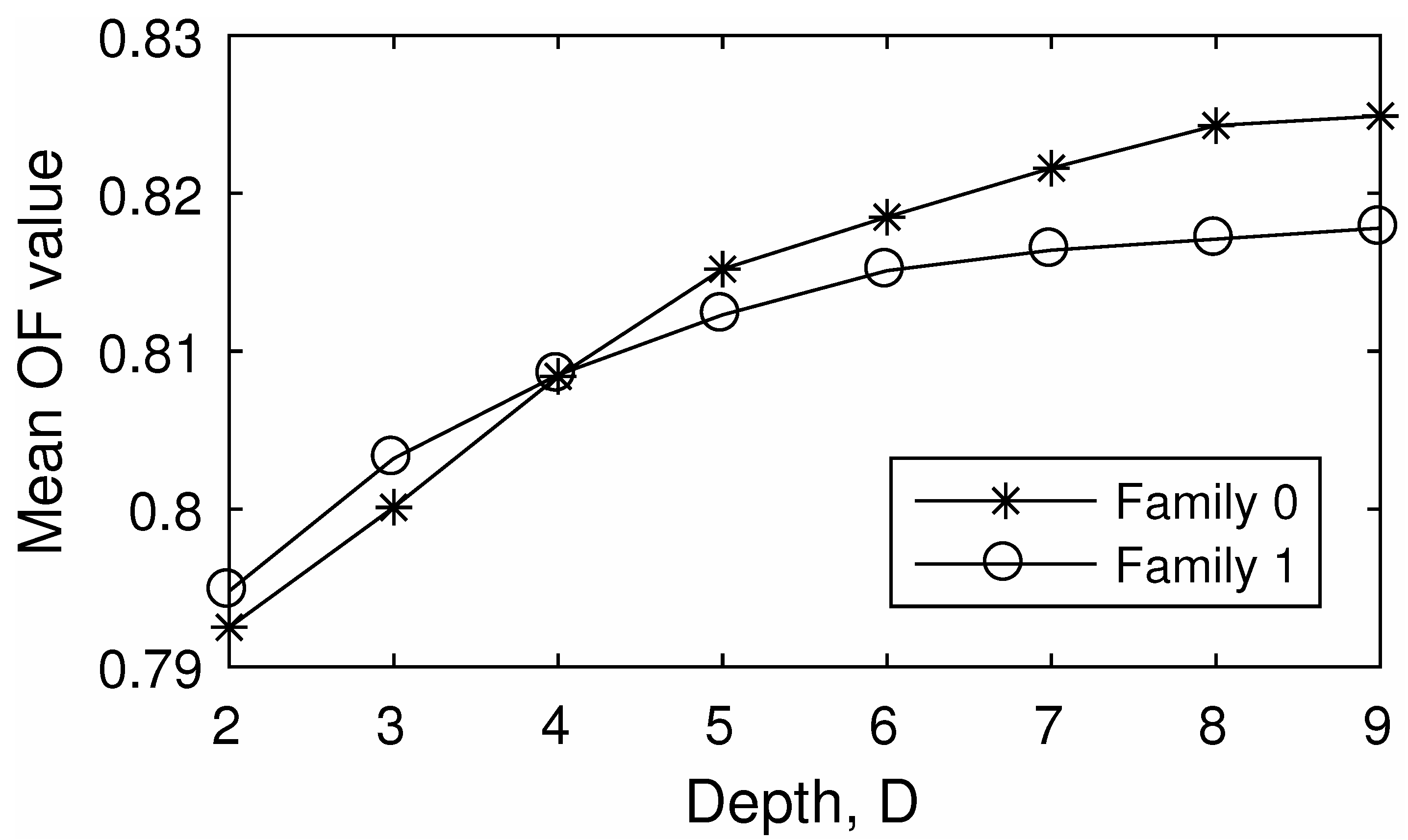
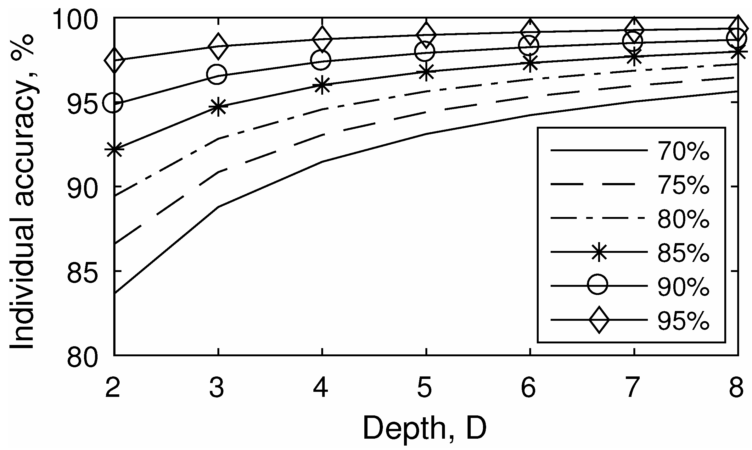
To achieve a null motion per simulation time-step $dt=0.01$, for a 20 s simulation, a length of $D=2000$ is required. Such a length is not practical for optimization and near real time applications in terms of execution time and numerical computations. To select a proper depth value, 26 different initial gimbal angles in the range of $[-\pi /2,\pi /2]$ and 60 different commanded quaternions that belong in the two first families are selected and the OF value are calculated for each combination of them. It is observed that increasing the depth further than 8 does not significantly improve the mean value of the OF as depicted in Figure 1, so $D=8$ is the preferable depth value.

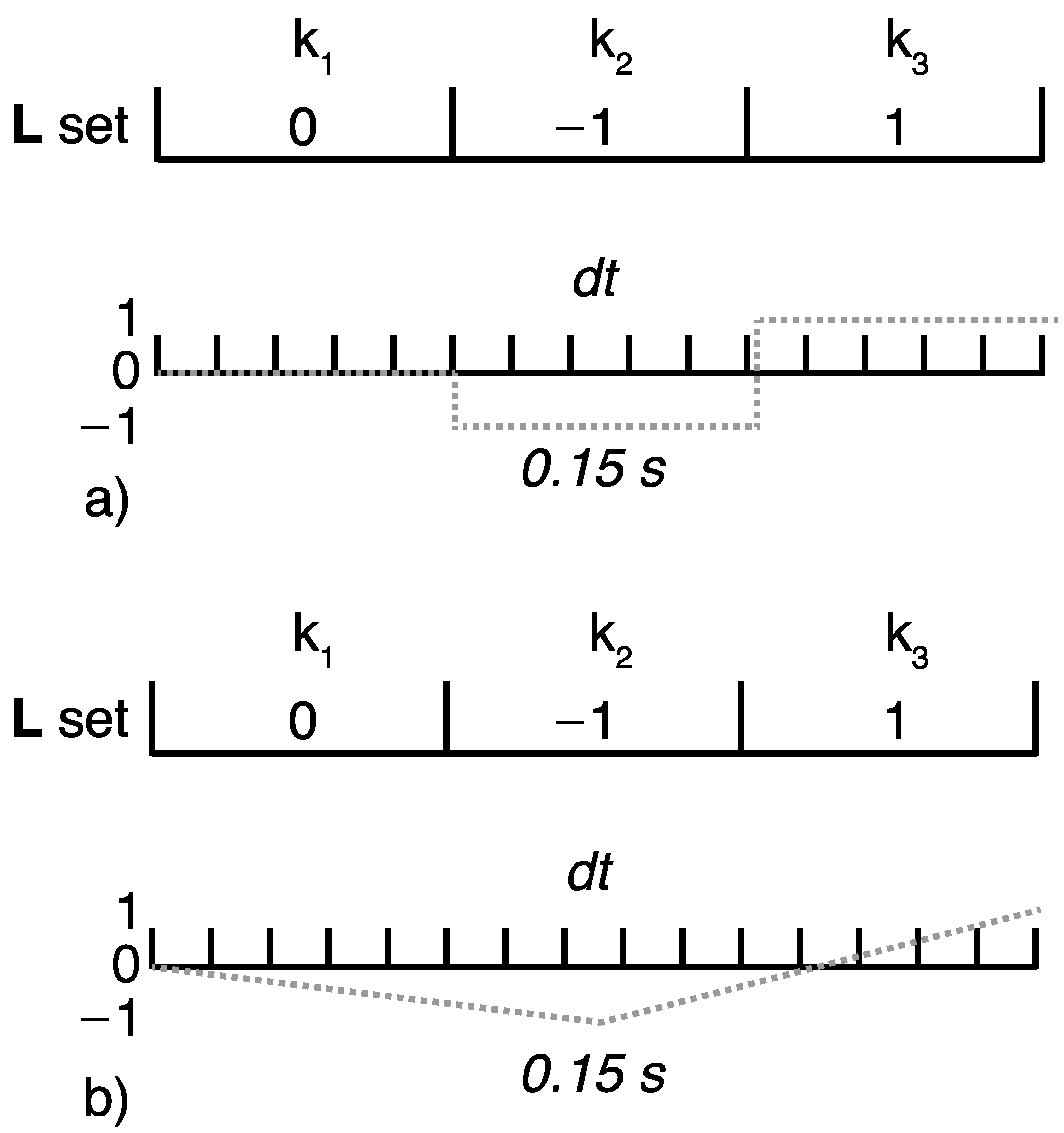
To match the simulation time-steps, the $\mathbf{L}$ set is interpolated through the simulation time. In Figure 2, two different approaches for interpolation are presented, as example for a total simulation time equal to 0.15 s and $D=3$. The first approach (Figure 2a) is similar to a Zero-Order-Hold (ZOH) filter, whilst the second (Figure 2b) is a linear interpolation. In this paper, the linear interpolation is used for simplicity.

For each gimbal set in a class, the optimization algorithm runs for a set of commanded quaternions in order to obtain the data-set. The commanded quaternions are converted from Euler angles to quaternions because it is easier to describe and comprehend a maneuver as a rotation about roll, pitch, and yaw. The maneuvers given are: independent rotation about roll, pitch, yaw for $\pi$/6, $\pi$/2, 2$\pi$/3, $\pi$, and all the possible permutations of two of those independent rotations.

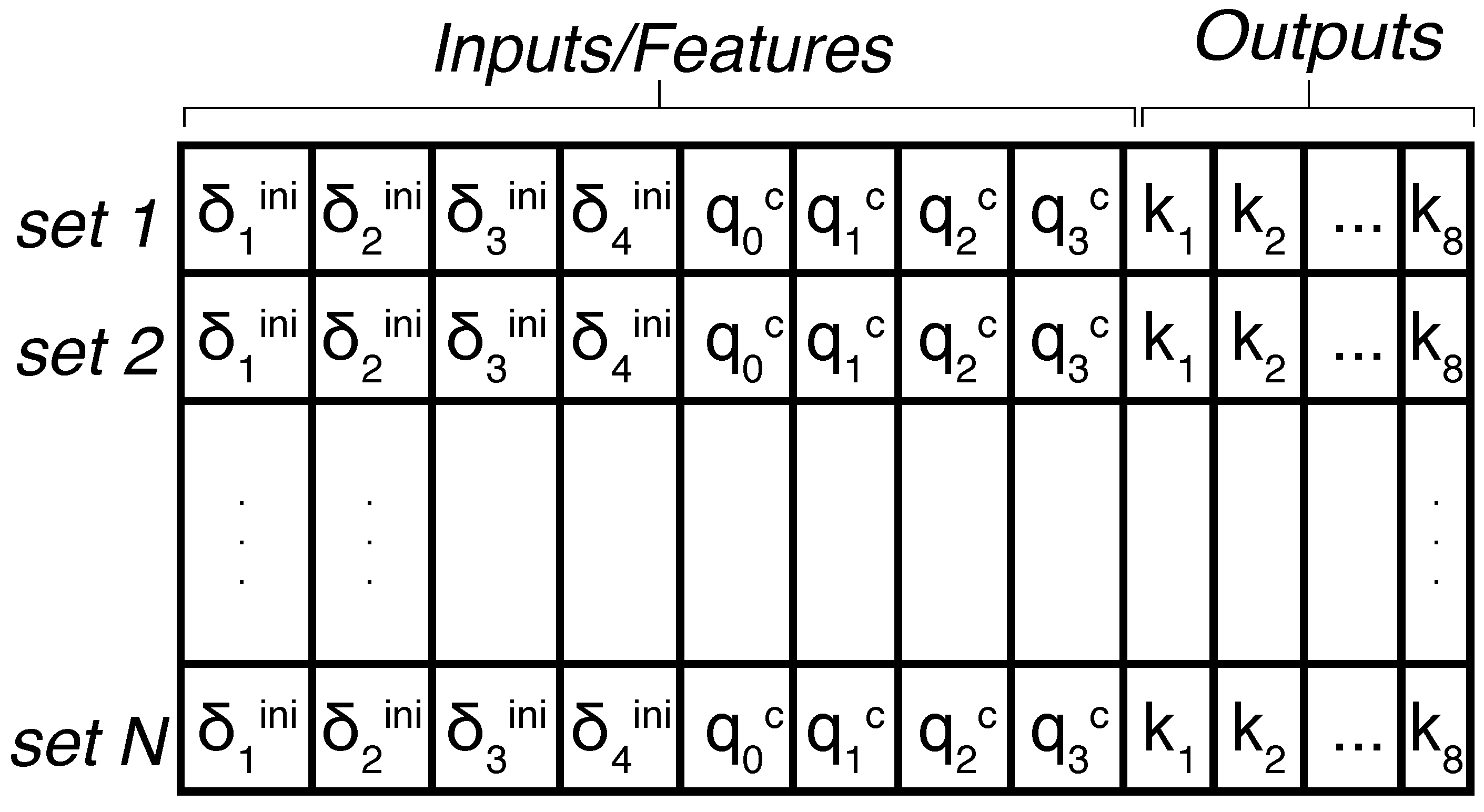
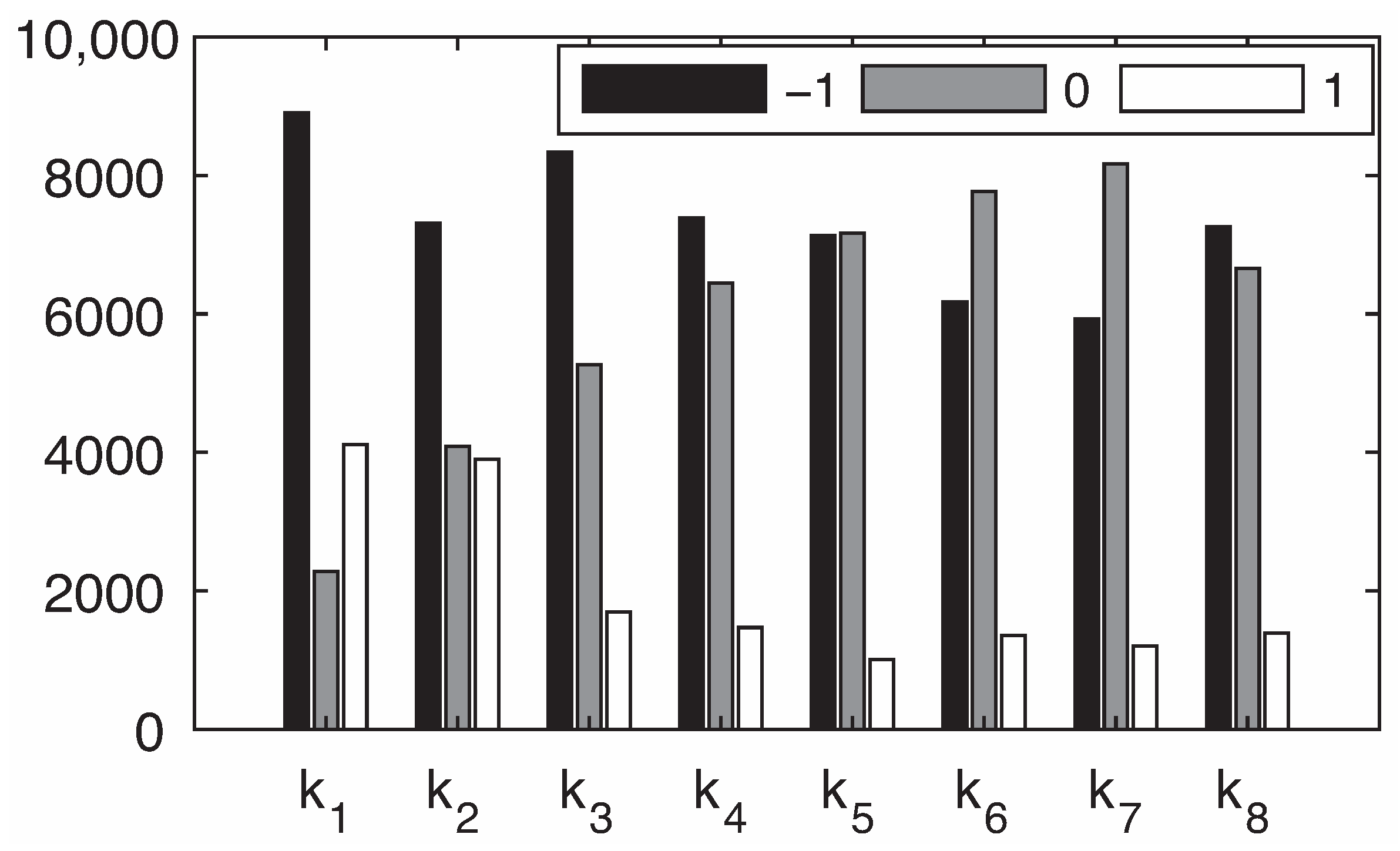
The structure of the data-set and the histogram of the different $k_i$ values for each element of $\mathbf{L}$ set are presented in Figure 3 and Figure 4, respectively.

It is observed that there is an unequal distribution between the values. The value 1 is observed the least in all elements, except for the first. The value −1 is the dominant value for the first four elements and the value 0 is dominant only for the the fifth element.

In a higher capability hardware, it would be feasible to use a larger set of commanded quaternions and more than three individual values to describe the motion in the null space. Moreover, including more values in the $\mathbf{L}$ set could better match the simulation time-steps, improving the interpolation results.

The exact simulation parameters used to produce the data-set are shown in

Table 2. Simulation Parameters.

Parameter	Value
Moment of Inertia J	$\mathrm{diag}\left(\right[1,1,1\left]\right)$${\mathrm{kgm}}^2$
Momentum $h_0$	1 Nms
Time-step dt	0.1 s
Simulation time	7 s
PID, $K_p$, $K_i$, $K_{\omega }$	20, ${10}^{-5}$, 15
Skew angle $\beta$	54.73 $\mathrm{deg}$
${\dot{\delta }}_{th}$	50 $\mathrm{deg}/\mathrm{s}$
$k_{max}$	0.7
D	8

.

4. Data Utilization

The data-set derived does not contain all the possible initial gimbal angles nor all the possible commanded quaternions. Hence, it is important to exploit those data to predict the value of the $\mathbf{L}$ set, even for these initial gimbal angles and commanded quaternions that are not included in the data-set. To do that, two different ML techniques are utilized. The input data in both techniques are standardized, i.e the values of each column are individually normalized so that each input data have $\mu =0$ and $\sigma =1$. A training data-set of $N=$ 15,300 different input samples is used to train the ML systems, whilst 765 different samples are used for validation. Without loss of generality, in this paper, only the Family 0 is studied due to hardware limitations and the long time required to derive the data-set for each class.

4.1. Deep Neural Network

The first technique is using eight different DNNs, each one to predict one element of the $\mathbf{L}$ set. The algorithm attempts to estimate the mapping function from the input variables to the categorical output variables. In contrast to convolutional neural networks that are used mainly in computer vision problems for image and video data, this paper presents the implementation of DNNs, for simplicity, which focuses more on how the information from input is represented via a set of non-linear functions. Each DNN has eight (8) neurons in the input layer, four (4) for the commanded quaternion, and four (4) for the initial gimbal angles. The $k_{max}$ value is constant and can be ignored in encoding the different $k_i$ values. Three bits are used for the categorical representations to create the three classes as $-1->[1,0,0]$, $0->[0,1,0]$, and $1->[0,0,1]$. Thus, the output layer of each DNN consists of three neurons which represent the $k_i$ as described in the previous section. The selection of the optimal DNN architecture is generally problem-dependent, and even though trial and error might work, there is no guarantee that it will lead to the optimal solution. Several studies have been done to optimize the topology of such networks, many of them making use of genetic algorithms [41,42,43]. Some rule-of-thumbs still exist that roughly determine some good DNN architectures. In [44], the number of hidden neurons $N_h$ for the first hidden layer is selected as $N_h=\sqrt{(m+2)N}+2\sqrt{N/(m+2)}$ and for the second hidden layers as $N_h=m\sqrt{N/(m+2)}$, where m is the number of output neurons and N is the number of sample data. The formula $N_h=(N_{in}+\sqrt{N})/L$ where L is the number of hidden layers and $N_{in}$ is the number of input neurons is also proposed [45]. Other methods have also been discussed in [46,47,48]. In this paper, three hidden layers are used, with 64 neurons in each one. It has been observed, through trial and error, that more neurons and layers not only increase the ML system complexity, requiring a longer training time, but also deteriorate the performance because of overfitting. There are 8 neurons in the input layer and 3 neurons in the output layer, as described earlier. Even though it is not feasible to reduce the input and output neurons, it is possible to further adjust the number of the hidden layers and their neurons. However, narrowing the network forces it to give up some information, while trying to keep as much relevant information as possible. The architecture of a single DNN to predict the whole L set reduces even more the reliability of the results compared to the 8 separate DNNs scheme. According to the universal approximation theorem [49], it is known that for the same problem, a network of only one hidden layer can be used, followed by different parameter tuning and number of neurons. In practice, however, it has been seen that a swallow network usually requires a large number of neurons to be useful; possibly much larger than this required by a deep network while they often present a lower performance in terms of convergence and local minima [50]. A visualization of the ith DNN model predicting the corresponding output $k_i$ is shown in Figure 5.

The activation function of each neuron in the input and hidden layers is the Rectified Linear Unit:

$$f\left(x\right)=\left\{\begin{array}{cc}0,\hfill & forx\le 0\hfill \\ x,\hfill & forx>0\hfill \end{array}\right.$$

(23)

The activation function for the neurons in the output layer is the sigmoid function:

$$f\left(x\right)=\frac{1}{1+e^{-x}}$$

(24)

The batch size of the DNN, which denotes the number of data samples that will be propagated through the network before updating the weights of the network, is equal to 64. Selecting the batch size is a trade off among less training time and better training results. The RMSprop algorithm [51] is implemented as the optimizer, the learning rate and the discounting factor of which are selected through trial and error in order to achieve the higher possible accuracy without overfitting. The epoch limit is set to 100 because no further improvement in accuracy is observed after this value. The categorical cross entropy loss function is used for multi-class classification, which is given by:

$$CCE=-\sum _{c=1}^z{y}_{i,c}log\left({\tau }_{i,c}\right)$$

(25)

where z is the number of classes, $y_{i,c}$ is 0 or 1, indicating whether the sample belongs to class c, and ${\tau }_{i,c}$ is the probability for this sample to belong in class c.

The accuracy of each DNN using the validation data is presented in

Table 3. DNNs—Accuracy.

DNN No.	Value%
DNN 1	80.8%
DNN 2	83.0%
DNN 3	77.5%
DNN 4	77.5%
DNN 5	76.6%
DNN 6	75.8%
DNN 7	74.2%
DNN 8	67.5%
Total	28.1%

.

The total accuracy is expected to be lower than the accuracy obtained by each DNN individually, because more than one independent values must be predicted correctly. The total accuracy measured by combining all the DNNs is 28.1%. Tuning the parameters of the DNNs differently or changing the size of the training and validation data-set does not significantly improve the results.

The fact that the number of output data of class 1 are fewer than the data of the rest classes for DNN3-DNN8 is partly responsible for the low total accuracy. Even if all DNNs had the accuracy of the first two DNNs, the final accuracy will not be high enough to make the predictions reliable. The total accuracy can be easily conceived as the product of the individual accuracies, even though in practice they are not identical. Thus, to obtain a high performance ML system for predictions, the individual predictions must be higher than the total accuracy, and as the depth D increases there is a demand for even higher individual accuracies (Figure 6). For example, to obtain a total accuracy of 85% for $D=3$, the individual accuracies required a reach up to 94.7%.

4.2. Random Forest Classifier

The second technique used is the RFC. In general, the RFC algorithm generates a large number of individual decision trees that operate as an ensemble. Each individual tree produces a class prediction and the class with the most votes becomes the ML system prediction. Each tree splits from parent to child node following a specific method. They split on the feature and corresponding split point that results in the largest Information Gain (IG) for a given criterion. Entropy is one of the most frequently used selection criteria for decision trees, and it is given by

$$I_H=-\sum _{j=1}^c{\tau }_j{log}_2\left({\tau }_j\right)$$

(26)

where ${\tau }_j$ is the proportion of the samples that belongs to class c for a particular node. The IG can be calculated as

$$IG\left(D_{\tau },f\right)=I\left(D_{\tau }\right)-\sum _{j=1}^m\frac{N_j}{N}I\left(D_j\right)$$

(27)

where f is the feature split on, $D_{\tau }$ the data-set of the parent node, $D_j$ the data-set of the jth child node, I the impurity criterion, N the total number of samples, and $N_j$ the number of samples at jth child node. 200 estimators are used because increasing the number of estimators above this value does not improve the resulting accuracy. All nodes are expanded until all children are pure. The RFC is studied using two approaches. In the first, the RFC is implemented to predict the whole $\mathbf{L}$ set at once given the input gimbal and quaternion values. In the second, the RFC predicts each value in L set individually. A visualization of the two RFC approaches is shown in Figure 7.

The maximum number of inputs the algorithm considers when looking for the best split is selected through trial and error to achieve the best accuracy. For the first approach, it is found to be equal to 7 and the accuracy in the validation data is 75.2%, with mean absolute error 0.098. Even though not all classes have an equivalent number of samples, the RFC is capable of predicting all three with enhanced accuracy.

In the second approach, each RFC is trained to predict each $k_i$ value individually, the number of estimators remains the same, and the maximum number of inputs is set to 3. Regardless of the RFC approach used, the RFC technique always presents a better accuracy compared to this obtained by the DNNs. The total accuracy for the second approach is equal to 71.8% and the mean squared error 0.109. The accuracies are shown in

Table 4. RFC—Accuracies.

RFC No.	Approach 1	Approach 2
RFC 1	94.0%	92.7%
RFC 2	93.1%	92.4%
RFC 3	91.8%	91.9%
RFC 4	93.3%	91.2%
RFC 5	93.3%	91.2%
RFC 6	91.2%	90.5%
RFC 7	91.1%	89.3%
RFC 8	87.3%	88.1%
Total	75.2%	71.8%

.

5. Simulation Results

After defining and training the ML systems, an initial gimbal angle set and a commanded quaternion are selected to predict the null space motion of the system and evaluate the performance of DNNs and RFC. The selected angle set is ${\delta }^{ini}={[{\delta }_1^{ini},{\delta }_2^{ini},{\delta }_3^{ini},{\delta }_4^{ini}]}^T={[0,0,0,0]}^T$ deg because it is easy to verify that it belongs to family 0. Without any loss of generality, the commanded maneuver is selected to be a rotation about one axis for simplicity, and the value of the commanded quaternion is selected randomly as ${\mathbf{q}}^c={[0.6178,-0.7863,0,0]}^T$ which corresponds to a −103.69 deg rotation about the roll axis. A 2.7 GHz Inter Core i5 with 8 GB of RAM computer was used and all the simulations were run on the operating system macOS Big Sur in Matlab^® R2016b.

For these inputs, the DNNs prediction is $k_{max}[-1,1,-1,0,0,0,0,0]$. The RFC prediction in the first approach is $k_{max}[1,1,-1,0,0,0,0,0]$, whilst in the second approach it is $k_{max}[-1,-1,-1,0,0,0,0,0]$. All three predictions have in common that the last five elements are zero. This is expected because the low performance configuration is encountered near the beginning of the simulation where the ML systems predict a non zero null space motion. After this state, there is no need for null motion, since every gimbal configuration after the singularity corresponds to a better performance index. As a result, the rest of the elements are zero. The gimbal rates and the manipulability index for each prediction are presented in Figure 8, Figure 9, Figure 10 and Figure 11 and the results of the null space projection (NSP) upon the Moore-Penrose pseudo-inverse are also shown for comparison. This NSP steering law is given by

$$\dot{\delta }={\mathbf{A}}^{\#}\dot{\mathbf{h}}+{\kappa }_{ns}({\mathbf{I}}_{4x4}-{\mathbf{A}}^{\#}\mathbf{A})\nabla w\left(\delta \right)$$

(28)

where ${\kappa }_{ns}$ is a constant gain equal to 2, ${\mathbf{I}}_{4x4}$ is the 4 by 4 identity matrix, and $\nabla w\left(\delta \right)$ indicates the gradient of the manipulability index with respect to the gimbal angles.

Similarly to most ML techniques, the derivation of the data-set and the training of the model can be done offline without being involved in the operation of the system. Thus, a total time comparison between the NSP and the ML techniques would be unfair. In order to measure the execution time difference, i.e the time it takes for all the calculations needed until the end of the simulation, the training and data-set derivation time are excluded.

Table 5. Execution time.

ML Model	Percentage
DNN	−50.9%
RFC 1	−51.1%
RFC 2	−48.4%

shows the percentage difference in the execution time with respect to the NSP. It is observed that there is a 50.9%, 51.1%, and 48.4% improvement in the execution time when the ML techniques are utilized compared to the NSP. This is expected because there is no need to calculate the gradient of the performance index of the Equation (28), which is the most time consuming part. The proposed ML methods offer the advantage of directly executing the null motion through commanding the $\mathbf{L}$ set to the CMG cluster. No need for additional computational power is required, since the model generation, the training, and the predictions of $k_i$ values are executed a priori.

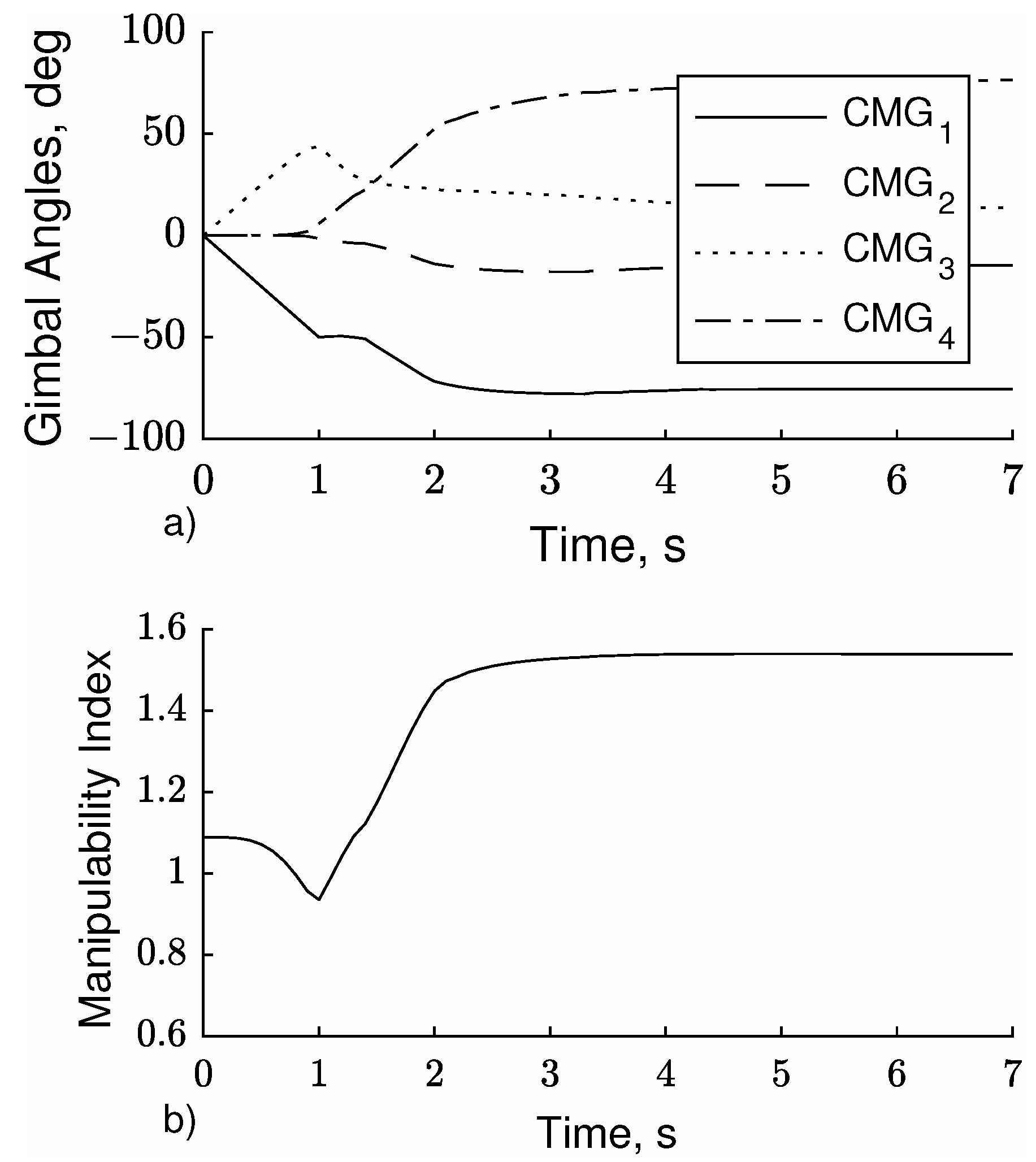
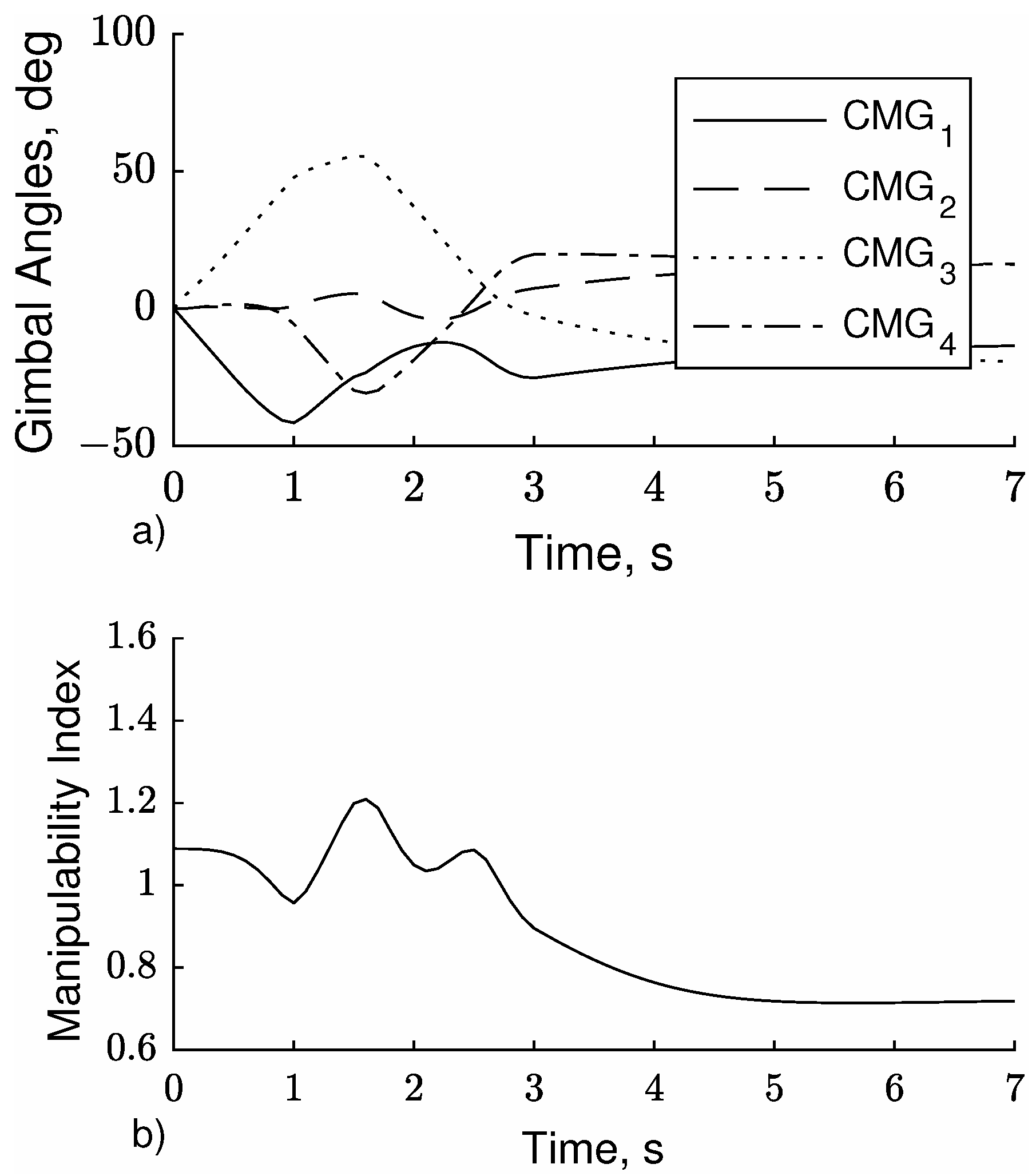
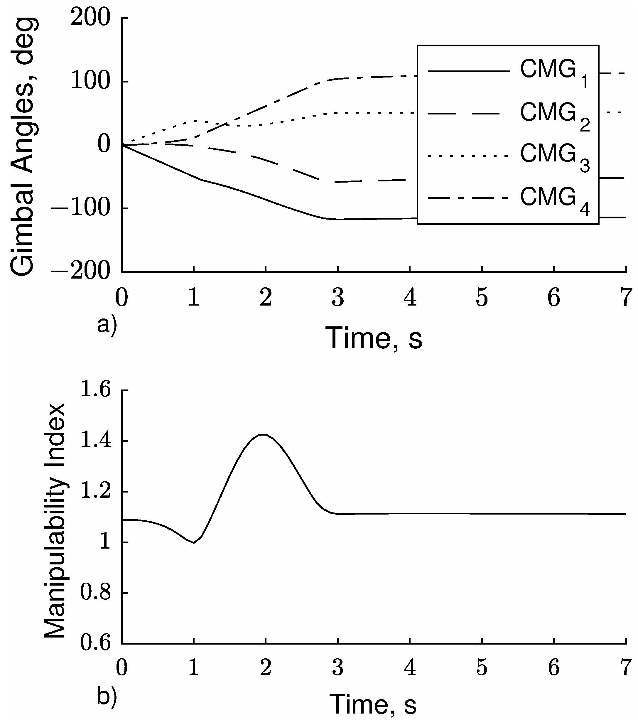
The gimbal angles and the manipulability index when the NSP is used are shown in Figure 8a,b respectively. At t = 1.1 s, the gimbal angles are $[-50,-1.4,43.7,5.9]$ deg and the minimum value of the manipulability index equals to 0.935 is obtained. In Figure 9a,b, the results for the null motion predicted by the DNNs are presented. The minimum value of the index equals to 0.7144 and is observed at t = 5.8 s when the gimbal angles configuration is $[-15.2,15.3,-17.7,17.1]$ deg. 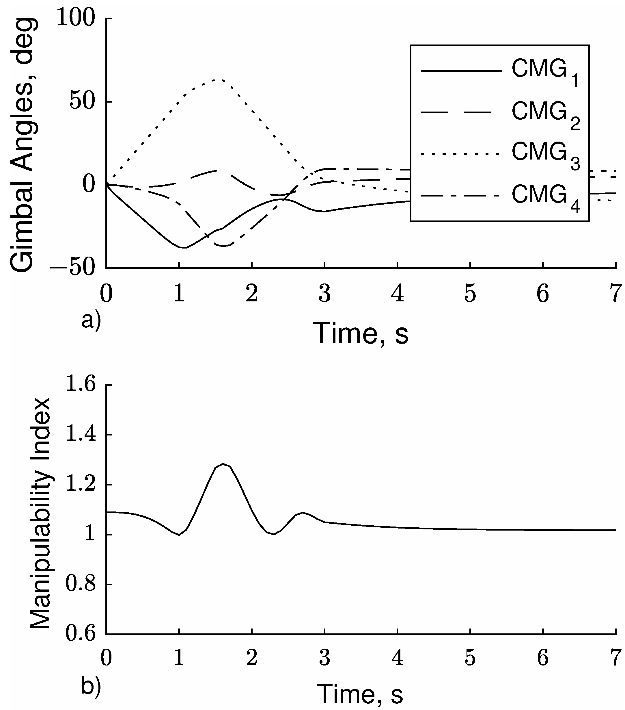Figure 10a,b illustrate the results for the null motion predicted by the first approach of the RFC. Similarly to the NSP, the minimum index value is obtained at t=1.1 s, but the configuration at this time is $[-37.5,1.5,50.0,-11.4]$ deg. This leads to a higher minimum index value, equal to 0.9978. The results for the second approach of the RFC can be seen in Figure 10b and Figure 11a. The minimum index value and the time it is obtained are the same as previously. However, significantly different gimbal angle profiles are presented that result in a higher manipulability maximum. In addition, constantly higher values are obtained after t = 3 s compared to the first approach of the RFC. It is expected that the NSP will present a higher performance index after the low performance configuration because it aims to improve the value of the manipulability index locally. In contrast, the ML techniques are implemented to exclusively maximize the minimum index value across the desired maneuver, not the performance index in each time-step. The main drawback of NSP is that it drives the system to higher performance configurations, exploring the possible movements in the gimbal space locally. Hence, it is possible to ignore a path in gimbal space that results in a higher minimum index value because the path locally decreases the manipulability index. Such problems are avoided with global steering approaches, as the techniques described in this paper. It is expected that the RFC approaches will present a lower manipulability index value after t = 1.1 s compared to NSP, when the system has overpassed the singularity. In contrast, the prediction made by DNNs results in a lower minimum manipulability value than this obtained by the NSP, indicating that the DNNs are unable to make useful predictions for the specific application. In terms of attitude error, all the maneuvers are executed with zero attitude error because the null space motion does not affect the attitude of the system.

It has been proven that the first approach of the RFC provides a gimbal angle trajectory, in the null space, which results in the highest minimum manipulability value while it has been shown that this RFC model results in the highest accuracy among the examined models. Even though NSP can be implemented on board, it has been shown that when the $\mathbf{L}$ set is commanded directly to the satellite, there is a significant improvement in the execution time required, as measured in the simulation.

The main downside of the proposed ML models is that they are limited by the physical characteristics of the system used to derive the training and the test data. In this paper, the identity matrix is selected as the inertia matrix of the satellite for simplicity, even though it is unrealistic. However, the complexity of the problem remains the same whether the inertia matrix is the identity matrix or a more complex matrix that depicts the characteristics of a satellite in a real-life application scenario. Moreover, selecting a higher value of D would allow to decide the null space motion in shorter time intervals, even though it would require more time to derive the data-set and train the ML model. Nonetheless, Figure 1 illustrates that increasing the depth values does not drastically improve the the mean OF value, which indicates the existence of a upper bound in the useful depth value. The various hyper-parameters associated with the ML implementation have to be selected according to the specific data, i.e., their number and reliability, because no universal tuning exists to fit every ML problem. The selection of these variables constitutes a research field, which is beyond the scope of this paper.

Despite the limited capabilities of the presented ML systems, due to hardware and time constraints, the described methodology provides significantly high scalability. It is possible to potentially provide a generalized predictive system by enriching the current data-set with more maneuvers, initial gimbal configurations, and different satellite inertias that can be used as data inputs. Thus, this methodology describes a way of developing both a training data-set and a predictive system for null motion path planning for a wide range of satellites. The OF can easily be adjusted to include more terms like the mean value of a manipulability index and/or the time the gimbal rates exceed a specific threshold. Such an approach would further increase the utility of the system in more realistic applications. In contrast to local gradient methods as NSP, global steering techniques provide the advantage of overcoming local extrema and it has been proved, as expected, that the presented method demands lower execution time since there is no need of calculating the gradient of the performance index in each iteration. Moreover, the interpolation of the L set through the simulation time provides a way of handling long maneuvers without the demand of producing a different null motion value for each step. Through the implementation of the gimbal families, it has been proved that a depth value of no more than eight is efficient for predicting the null motion path.

6. Conclusions

This paper constitutes a framework for approaching the Control Moment Gyroscope (CMG) cluster singularity problem using Machine Learning (ML) techniques. Two ML techniques for global steering the pyramid-type 4-CMG cluster have been investigated. A novel heuristic algorithm has been developed that calculates the optimal null space motion path, taking into consideration a manipulability-based Objective Function (OF) through the whole maneuvers, given the initial gimbal angles of each CMG and the commanded quaternion. The generated data-set that relates the initial gimbal angles and the commanded quaternion to the null space motion is used to train two ML systems. Among the two ML techniques, the Random Forest Classifier (RFC) presents the best performance, predicting with efficient accuracy the desired null space motion, even for maneuvers that are not included in the training set. A task is selected to evaluate the performance of the system following the predicted null motion derived by each ML technique, and the results verify that the RFC presents a higher minimum manipulability index compared to the Null Space Projection. Overall, this study is encouraging the determination of a singularity-free maneuver that can be known a priori and provides the utilization of gimbal families for the classification of the gimbal angles. The proposed methodology can be easily adapted to a wide range of satellites as long as their dynamic model is known, otherwise, the same procedure can be followed only for the kinematics model. In conjunction with an inspection mechanism, it is possible to monitor whether the real system follows the prediction. In case of deviations (e.g., produced by external disturbances), a new prediction can be obtained using, as initial/input configuration, the current configuration. Moreover, once the data-set is created and the training of the ML system has been completed, the computational demands to predict the output are significantly low, suggesting that the trained system can be potentially used on board to predict the desired $\mathbf{L}$ set in real-time. However, the implementation and the needs of such an approach are beyond the scope of this paper and they are reserved for future work. Additional research should focus on enhancing the predictions using other types of neural networks, such as 1-D convolutional neural networks or long short-term memory networks, while assessing the performance of the system for the partially correct predictions in an effort to utilize them in case they do not deteriorate the OF.

References

1. Roser, X.; Sghedoni, M. Control Moment Gyroscopes (CMG’s) and their Application in Future Scientific Missions. In Spacecraft Guidance, Navigation and Control Systems; Kaldeich-Schuermann, B., Ed.; European Space Agency (ESA) Special Publication: Noordwijk, The Netherlands, 1997; Volume 381, p. 523. [Google Scholar]
2. Defendini, A.; Lagadec, K.; Guay, P.; Blais, T.; Griseri, G. Low Cost CMG-Based AOCS Designs. In Spacecraft Guidance, Navigation and Control Systems; Schürmann, B., Ed.; European Space Agency (ESA) Special Publication: Noordwijk, The Netherlands, 2000; Volume 425, p. 393. [Google Scholar]
3. Wie, B. Space Vehicle Dynamics and Control; American Institute of Aeronautics and Astronautics: Reston, VA, USA, 2008. [Google Scholar] [CrossRef]
4. Leve, F.A.; Hamilton, B.J.; Peck, M.A. Spacecraft Momentum Control Systems; Springer International Publishing: Berlin/Heidelberg, Germany, 2015; pp. 1–247. [Google Scholar] [CrossRef]
5. Bang, Y.; Choi, H.D. Attitude control of a bias momentum satellite using moment of inertia. IEEE Trans. Aerosp. Electron. Syst. 2002, 38, 243–250. [Google Scholar] [CrossRef]
6. Lian, B.; Bang, H. Momentum transfer-based attitude control of spacecraft with backstepping. IEEE Trans. Aerosp. Electron. Syst. 2006, 42, 453–463. [Google Scholar] [CrossRef]
7. Margulies, G.; Aubrun, J.N. Geometric Theory of Single-Gimbal Control Moment Gyro Systems. J. Astronaut. Sci. 1978, 26, 159–191. [Google Scholar]
8. Yoshikawa, T. Manipulability of Robotic Mechanisms. Int. J. Robot. Res. 1985, 4, 3–9. [Google Scholar] [CrossRef]
9. Kojima, H. Calculation and fitting of boundaries between elliptic and hyperbolic singularities of pyramid-type control moment gyros. Acta Astronaut. 2014, 104, 33–44. [Google Scholar] [CrossRef]
10. Guo, J.; Wu, B.; Geng, Y.; Kong, X.; Hou, Z. Rapid SGCMGs Singularity-Escape Steering Law in Gimbal Angle Space. IEEE Trans. Aerosp. Electron. Syst. 2018, 54, 2509–2525. [Google Scholar] [CrossRef]
11. Kurokawa, H. Exact singularity avoidance control of the pyramid type CMG system. In Proceedings of the Guidance, Navigation, and Control Conference, American Institute of Aeronautics and Astronautics, Scottsdale, AZ, USA, 1–3 August 1994; pp. 170–180. [Google Scholar] [CrossRef]
12. Leve, F.A.; Fitz-Coy, N.G. Hybrid Steering Logic for Single-Gimbal Control Moment Gyroscopes. J. Guid. Control Dyn. 2010, 33, 1202–1212. [Google Scholar] [CrossRef]
13. Wie, B. Singularity Escape/Avoidance Steering Logic for Control Moment Gyro Systems. J. Guid. Control Dyn. 2005, 28, 948–956. [Google Scholar] [CrossRef]
14. Wie, B.; Bailey, D.; Heiberg, C. Singularity Robust Steering Logic for Redundant Single-Gimbal Control Moment Gyros. J. Guid. Control Dyn. 2001, 24, 865–872. [Google Scholar] [CrossRef]
15. Vadali, S.R.; Walker, S.R.; OH, H.S. Preferred gimbal angles for single gimbal control moment gyros. J. Guid. Control Dyn. 1990, 13, 1090–1095. [Google Scholar] [CrossRef]
16. Geshnizjani, R.; Kornienko, A.; Ziegler, T.; Loehr, J.; Fichter, W. Optimal Initial Gimbal Angles for Agile Slew Maneuvers with Control Moment Gyroscopes. In Proceedings of the AIAA Scitech 2019 Forum, San Diego, CA, USA, 7–11 January 2019; American Institute of Aeronautics and Astronautics: Reston, VA, USA, 2019; pp. 1–10. [Google Scholar] [CrossRef]
17. Nanamori, Y.; Takahashi, M. Steering law of control moment gyros using optimization of initial gimbal angles for satellite attitude control. J. Syst. Des. Dyn. 2008, 74, 2698–2704. [Google Scholar] [CrossRef] [Green Version]
18. Paradiso, J. A Search-Based Approach to Steering Single Gimballed CMGs; Draper Laboratory: Cambridge, MA, USA, 1991. [Google Scholar]
19. Paradiso, J.A. Global steering of single gimballed control moment gyroscopes using a directed search. J. Guid. Control. Dyn. 1992, 15, 1236–1244. [Google Scholar] [CrossRef]
20. Papakonstantinou, C.; Lappas, V.J.; Schaub, H.; Kostopoulos, V. Global Steering for Control Moment Gyroscope Clusters Using Heuristic Variable Search Techniques. J. Spacecr. Rocket. 2021, 58, 972–983. [Google Scholar] [CrossRef]
21. Qian, Z.; Guojin, T. Technical Note: Space Station Zero Propellant Maneuver Path Planning Considering SGCMG Saturation and Singularity. J. Astronaut. Sci. 2014, 61, 305–318. [Google Scholar] [CrossRef]
22. Jia, Y.; Misra, A.K. Trajectory Planning for a Space Robot Actuated by Control Moment Gyroscopes. J. Guid. Control Dyn. 2018, 41, 1838–1842. [Google Scholar] [CrossRef]
23. Geng, Y.; Hou, Z.; Huang, S. Global Singularity Avoidance Steering Law for Single-Gimbal Control Moment Gyroscopes. J. Guid. Control Dyn. 2017, 40, 3027–3036. [Google Scholar] [CrossRef]
24. Cui, P.; He, J.; Cui, J.; Li, H. Improved Path Planning and Attitude Control Method for Agile Maneuver Satellite with Double-Gimbal Control Moment Gyros. Math. Probl. Eng. 2015, 2015, 878724. [Google Scholar] [CrossRef]
25. Rosenblatt, F. The Perceptron, a Perceiving and Recognizing Automaton Project Para; Cornell Aeronautical Laboratory, Cornell Aeronautical Laboratory: Buffalo, NY, USA, 1957. [Google Scholar]
26. Pritt, M.; Chern, G. Satellite Image Classification with Deep Learning. In Proceedings of the 2017 IEEE Applied Imagery Pattern Recognition Workshop (AIPR), Washington, DC, USA, 10–12 October 2017; IEEE: Manhattan, NY, USA, 2017; pp. 1–7. [Google Scholar] [CrossRef]
27. Cornejo-Bueno, L.; Casanova-Mateo, C.; Sanz-Justo, J.; Salcedo-Sanz, S. Machine learning regressors for solar radiation estimation from satellite data. Sol. Energy 2019, 183, 768–775. [Google Scholar] [CrossRef]
28. Ferreira, P.V.R.; Paffenroth, R.; Wyglinski, A.M.; Hackett, T.M.; Bilén, S.G.; Reinhart, R.C.; Mortensen, D.J. Multiobjective Reinforcement Learning for Cognitive Satellite Communications Using Deep Neural Network Ensembles. IEEE J. Sel. Areas Commun. 2018, 36, 1030–1041. [Google Scholar] [CrossRef]
29. Leeghim, H.; Kim, D. Adaptive neural control of spacecraft using control moment gyros. Adv. Space Res. 2015, 55, 1382–1393. [Google Scholar] [CrossRef]
30. MacKunis, W.; Leve, F.; Patre, P.; Fitz-Coy, N.; Dixon, W. Adaptive neural network-based satellite attitude control in the presence of CMG uncertainty. Aerosp. Sci. Technol. 2016, 54, 218–228. [Google Scholar] [CrossRef]
31. Wu, Z.; Chou, W.; Wei, K. Steering Law Design for Single Gimbal Control Moment Gyroscopes Based on RBF Neural Networks. In PRICAI 2006: Trends in Artificial Intelligence; Yang, Q., Webb, G., Eds.; Springer: Berlin/Heidelberg, Germany, 2006; pp. 1186–1190. [Google Scholar] [CrossRef]
32. Moreno–Valenzuela, J.; Montoya–Cháirez, J.; Santibáñez, V. Robust trajectory tracking control of an underactuated control moment gyroscope via neural network–based feedback linearization. Neurocomputing 2020, 403, 314–324. [Google Scholar] [CrossRef]
33. Lungu, M.; Lungu, R. Adaptive Neural Network-Based Satellite Attitude Control by Using the Dynamic Inversion Technique and a VSCMG Pyramidal Cluster. Complexity 2019, 2019, 1645042. [Google Scholar] [CrossRef]
34. Enders, N. Deep Reinforcement Learning Applied To Spacecraft Attitude Control And Moment Of Inertia Estimation Via Recurrent Neural Networks. Master’s Thesis, Department of Aeronautics and Astronautics, Graduate School of Engineering and Management, Air Force Institute of Technology, Wright-Patterson Air Force Base, OH, USA, 2021. [Google Scholar]
35. Li, Y.; Hu, Q.; Shao, X. Neural network-based fault diagnosis for spacecraft with single-gimbal control moment gyros. Chin. J. Aeronaut. 2021. [Google Scholar] [CrossRef]
36. Berdugo, D.F.G. Application of Reinforcement Learning for the Control of a Control Moment Gyroscope. Master’s Thesis, Mechanical Engineering Universidad de Los Andes, Bogotá, Colombia, 2016. [Google Scholar]
37. Wu, B.; Wang, D.; Poh, E.K. High Precision Satellite Attitude Tracking Control via Iterative Learning Control. J. Guid. Control. Dyn. 2015, 38, 528–534. [Google Scholar] [CrossRef]
38. Wang, Q.; Psillakis, H.E.; Sun, C. Cooperative Control of Multiple High-Order Agents With Nonidentical Unknown Control Directions Under Fixed and Time-Varying Topologies. IEEE Trans. Syst. Man Cybern. Syst. 2021, 51, 2582–2591. [Google Scholar] [CrossRef]
39. Lappas, V.J. A Control Moment Gyro (CMG) Based Attitude Control System (ACS) for agile Small Satellites. Ph.D. Thesis, University of Surrey, School of Electronics and Physical Sciences, Guildford Surrey, UK, 2002. [Google Scholar]
40. Wie, B. Singularity Analysis and Visualization for Single-Gimbal Control Moment Gyro Systems. J. Guid. Control Dyn. 2004, 27, 271–282. [Google Scholar] [CrossRef]
41. Delgado, M.; Pegalajar, M. A multiobjective genetic algorithm for obtaining the optimal size of a recurrent neural network for grammatical inference. Pattern Recognit. 2005, 38, 1444–1456. [Google Scholar] [CrossRef]
42. Idrissi, M.A.J.; Ramchoun, H.; Ghanou, Y.; Ettaouil, M. Genetic algorithm for neural network architecture optimization. In Proceedings of the 2016 3rd International Conference on Logistics Operations Management (GOL), Fez, Morocco, 23–25 May 2016; IEEE: Manhattan, NY, USA, 2016; pp. 1–4. [Google Scholar] [CrossRef]
43. Arifovic, J.; Gençay, R. Using genetic algorithms to select architecture of a feedforward artificial neural network. Phys. A Stat. Mech. Its Appl. 2001, 289, 574–594. [Google Scholar] [CrossRef]
44. Huang, G.B. Learning capability and storage capacity of two-hidden-layer feedforward networks. IEEE Trans. Neural Netw. 2003, 14, 274–281. [Google Scholar] [CrossRef] [Green Version]
45. Ke, J.; Liu, X. Empirical Analysis of Optimal Hidden Neurons in Neural Network Modeling for Stock Prediction. In Proceedings of the 2008 IEEE Pacific-Asia Workshop on Computational Intelligence and Industrial Application, Wuhan, China, 19–20 December 2008; IEEE: Manhattan, NY, USA, 2008; Volume 2, pp. 828–832. [Google Scholar] [CrossRef]
46. Shibata, K.; Yusuke Ikeda. Effect of number of hidden neurons on learning in large-scale layered neural networks. In Proceedings of the ICCAS-SICE 2009—ICROS-SICE International Joint Conference 2009, Fukuoka, Japan, 18–21 August 2009; pp. 5008–5013. [Google Scholar]
47. Doukim, C.A.; Dargham, J.A.; Chekima, A. Finding the number of hidden neurons for an MLP neural network using coarse to fine search technique. In Proceedings of the 10th International Conference on Information Science, Signal Processing and their Applications (ISSPA 2010), Kuala Lumpur, Malaysia, 10–13 May 2010; IEEE: Manhattan, NY, USA, 2010; pp. 606–609. [Google Scholar] [CrossRef]
48. Yuan, H.; Xiong, F.; Huai, X. A method for estimating the number of hidden neurons in feed-forward neural networks based on information entropy. Comput. Electron. Agric. 2003, 40, 57–64. [Google Scholar] [CrossRef]
49. Cybenko, G. Approximation by superpositions of a sigmoidal function. Math. Control Signals Syst. 1989, 2, 303–314. [Google Scholar] [CrossRef]
50. Goodfellow, I.; Bengio, Y.; Courville, A. Deep Learning; MIT Press: Cambridge, MA, USA, 2016; Available online: http://www.deeplearningbook.org (accessed on 2 January 2022).
51. Team, K. Keras Documentation: RMSprop. Keras. Available online: https://keras.io/api/optimizers/rmsprop/ (accessed on 2 January 2022).
Figure 1. Minimum value of OF according to depth D for Family 0 and Family 1.
Aerospace 09 00164 g001
Figure 2. Interpolation approaches. (a) ZOH and (b) Linear.
Aerospace 09 00164 g002
Figure 3. Data-set structure.
Aerospace 09 00164 g003
Figure 4. Histogram of k i values.
Aerospace 09 00164 g004
Figure 5. Visualization of the DNN model.
Aerospace 09 00164 g005
Figure 6. Individual accuracies according to total accuracy.
Aerospace 09 00164 g006
Figure 7. Visualization of the RFC, (a) 1st and (b) 2nd approach.
Aerospace 09 00164 g007
Figure 8. Simulation results with NSP. (a) Gimbal angles, (b) Manipulability index.
Aerospace 09 00164 g008
Figure 9. Simulation results with DNN. (a) Gimbal angles, (b) Manipulability index.
Aerospace 09 00164 g009
Figure 10. Simulation results with RFC—1st approach. (a) Gimbal angles, (b) Manipulability index.
Aerospace 09 00164 g010
Figure 11. Simulation results with RFC—2nd approach. (a) Gimbal angles, (b) Manipulability index.
Aerospace 09 00164 g011