
Short-Term Trajectory Prediction Based on Hyperparametric Optimisation and a Dual Attention Mechanism


Abstract
:1. Introduction
- Kinetic models: Kinetic-based trajectory prediction models focus on the relationship between the forces acting on an aircraft and their motion. Zhang et al. [7] reduced the uncertainty of trajectory prediction by analysing model construction, aircraft intent, performance parameters, and other factors. Based on BADA data, He et al. [8] established a model for the change in parameters such as dynamics, meteorology, and flight path to achieve accurate trajectory prediction. Kang et al. [9] established an aircraft mass estimation model and an altitude profile prediction model based on real-time trajectory data. Lee et al. [10] proposed a stochastic system tracking model and an estimated-time-of-arrival prediction algorithm to construct a nonlinear dynamic model under multiple flight modes. Dynamical models require many parameters owing to the consideration of information such as aircraft performance, some of which are commercially sensitive, and others are obtained using estimates from existing databases. The prediction accuracy of the model is significantly reduced when the data resources are limited.
- State estimation model: The actual flight process can be considered a state transfer. Trajectory prediction estimates the state, such as latitude, longitude, and altitude, generated by the model during the flight. Chen et al. [11] constructed aircraft state equations based on known flight trajectory points, and they completed accurate trajectory prediction using an unscented Kalman filter. Lv et al. [12] improved the current Kalman filter (MIEKF) prediction system using multi-information theory to predict 4D trajectory in different states accurately. Zhou et al. [13] used the Kalman filter for track prediction, which is more suitable for single-step prediction than other models with significant short-term predictions. Tang et al. [14] used the IMM algorithm to track the aircraft’s trajectory using a geodetic coordinate system to represent the aircraft’s position and build each directional sub-model separately. The state estimation model is relatively simple, but it can lead to large errors owing to the inability to capture aircraft manoeuvre uncertainty accurately over long periods.
- Machine learning-based model: Machine learning has achieved great success in speech recognition, style migration, and image classification. Therefore, machine learning has also been applied to time-series data processing. Examples include pedestrian and vessel trajectory and traffic flow predictions [15,16,17]. Trajectory clustering is a clustering analysis of historical trajectories [18,19] that combines updated state information to correct prediction results and improve the prediction accuracy. Yin et al. [20] constructed a four-dimensional trajectory prediction model by analysing wind data in GRIB format. Pang et al. [21] proposed a Convolutional LSTM (ConvLSTM) to extract important features from weather information to solve pre-takeoff and convective weather-related trajectory prediction problems. Chen et al. [22] proposed a trajectory prediction model based on the attention mechanism and generative adversarial network to address problems such as the inability of the LSTM network to extract key information effectively for trajectory prediction. Shi et al. [23] proposed an online updated LSTM short-term prediction algorithm to address the influence of different factors in the navigation process on the current trajectory. Wang et al. [24] designed a training model with different K values and obtained an optimal parametric model by comparing the accuracies of different K values. Currently, LSTM neural networks are primarily used for trajectory prediction [25,26,27,28]. Hybrid models of CNN-LSTM are also widely used for prediction tasks [29,30]; however, these models have problems such as insufficient extraction of important features.
- a.
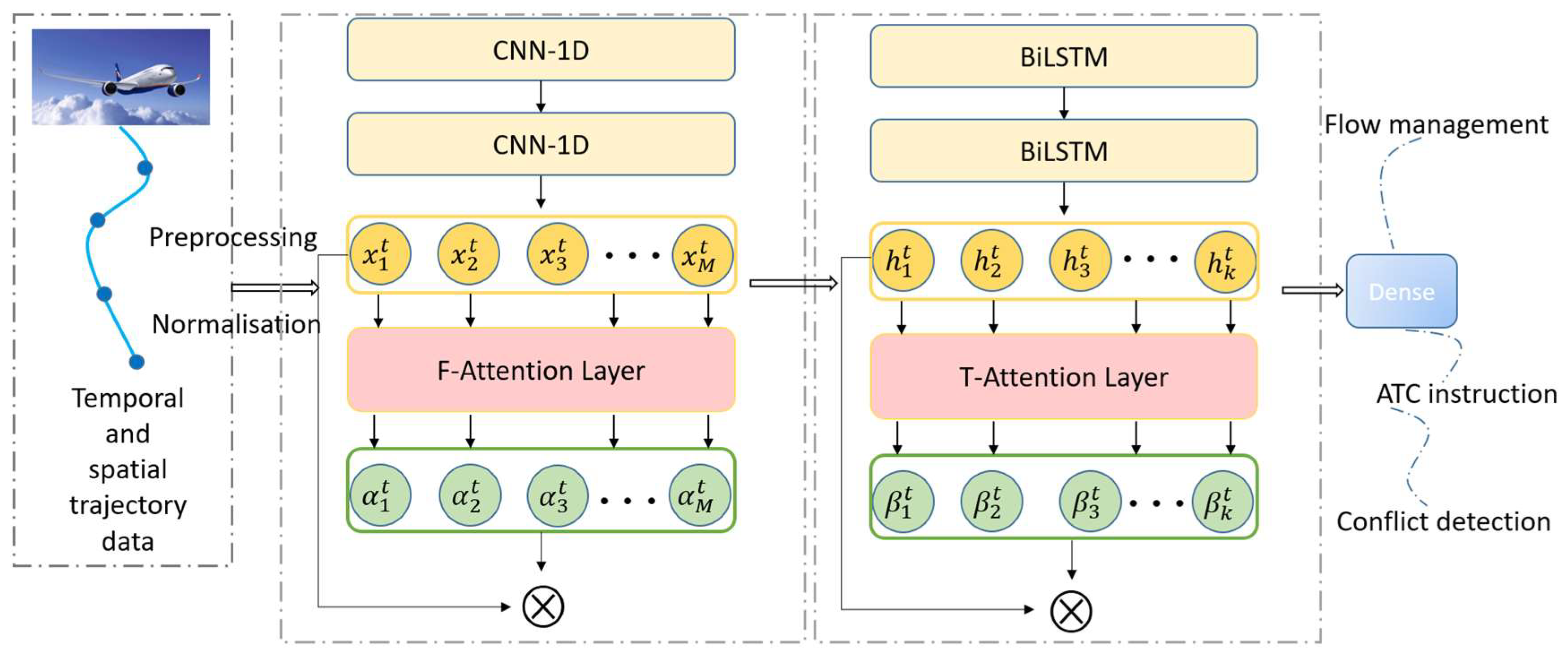
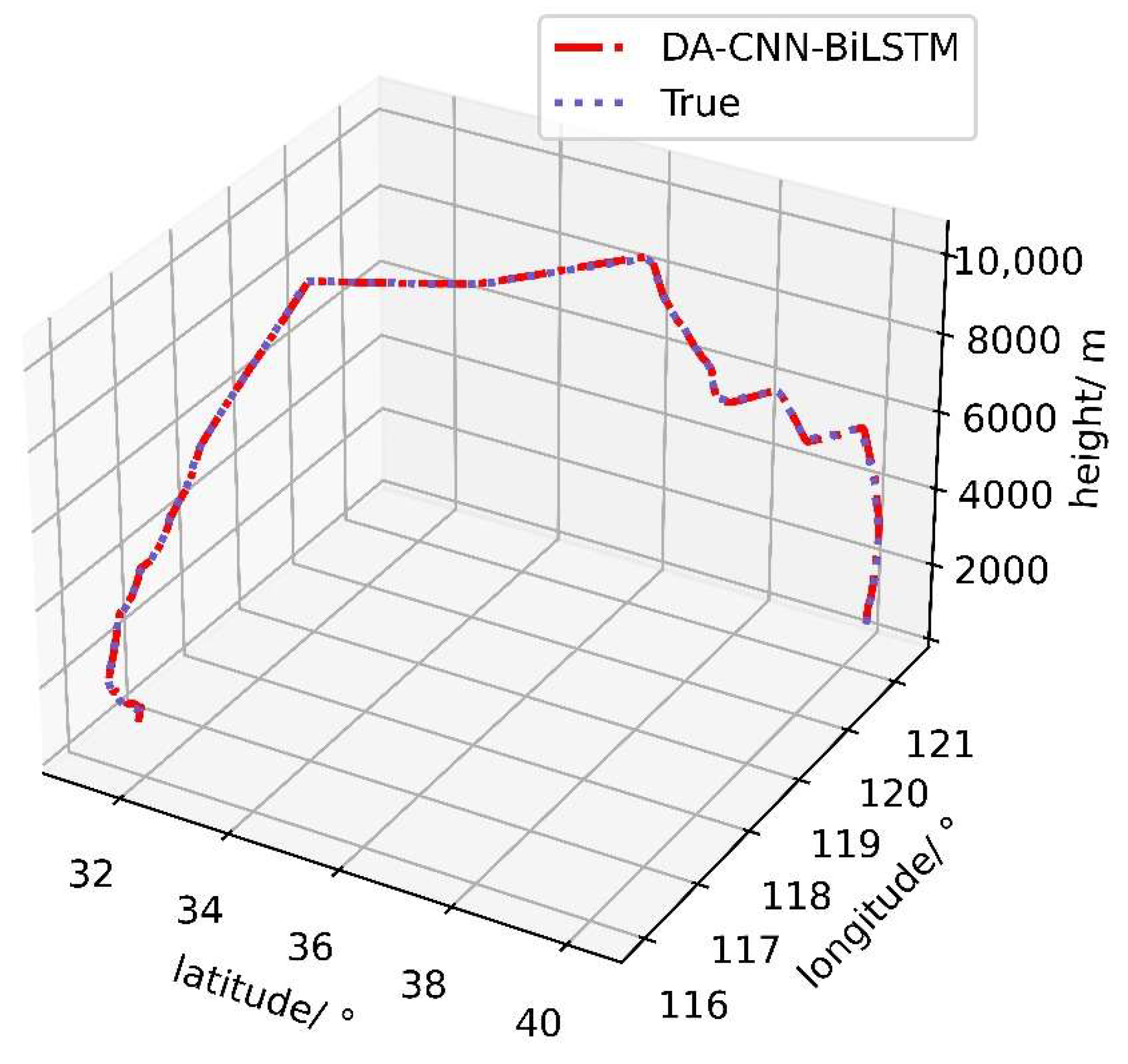
- By introducing the dual attention mechanism into the convolutional-bidirectional long short-term memory network (CNN-BiLSTM) model, the CNN was used to extract the trajectory space features, and the feature attention module achieved the mining of important features in the raw data and enhanced their impact by weighting the distribution of the CNN output. The subsequent BiLSTM module mines the trajectory temporal features, and the temporal attention module extracts important historical information based on the influence of each time node in the hidden layer state of the BiLSTM on the forecasting results, enhancing the learning of interdependencies in the time step. Thus, full integration of temporal features at the prediction points was achieved. The problem of important high-dimensional feature extraction and the long-term dependence of the time series was effectively solved. To the best of our knowledge, this is the first application of the DA-CNN-BiLSTM model to trajectory prediction.
- b.
- The use of genetic algorithms (GA) to optimise the hyperparameters of the entire model ensures the optimal learning capability of the model, overcoming the shortcomings of manual parameter tuning, which is experience-dependent, time-consuming, and has poor stability.
- c.
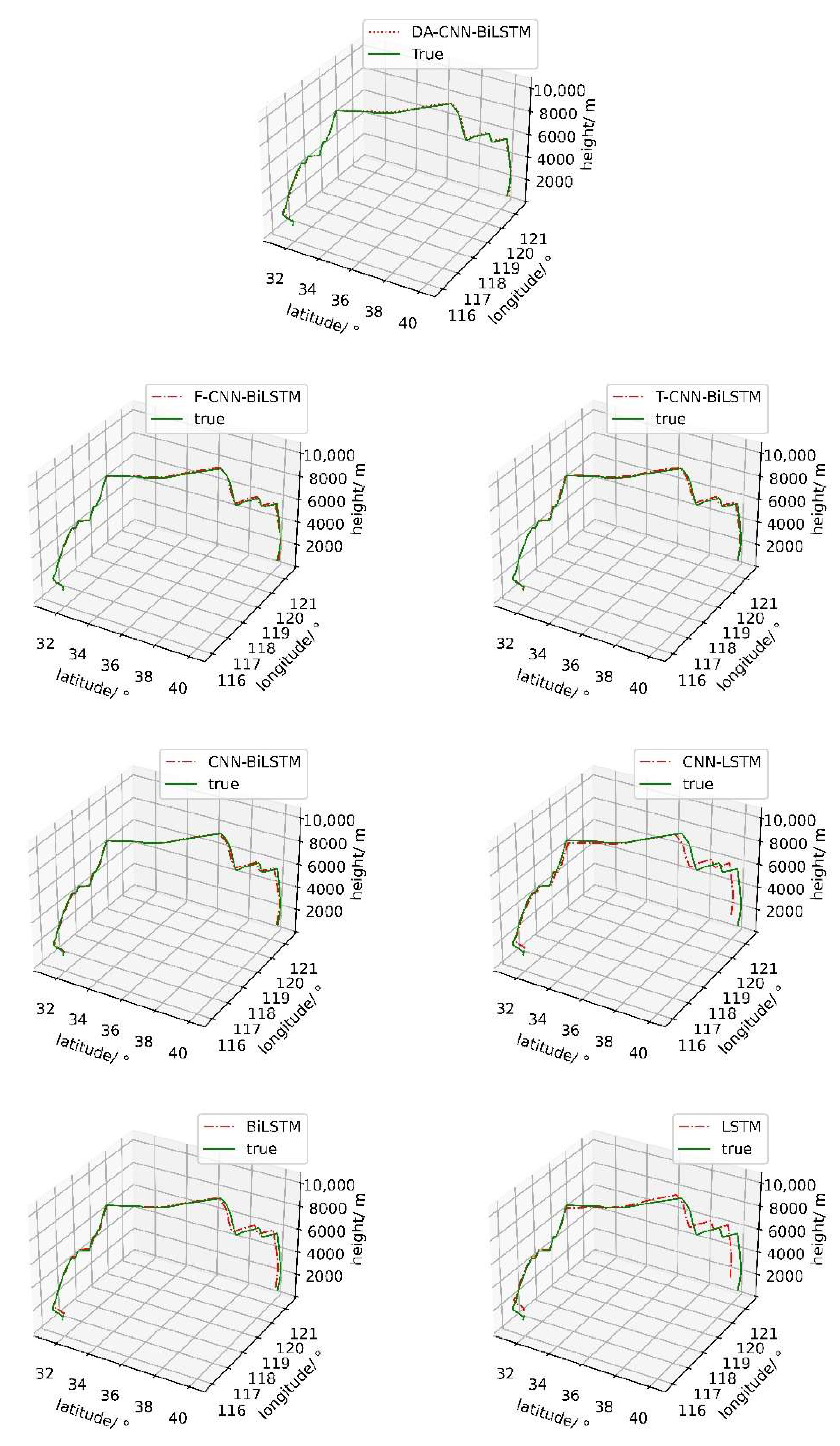
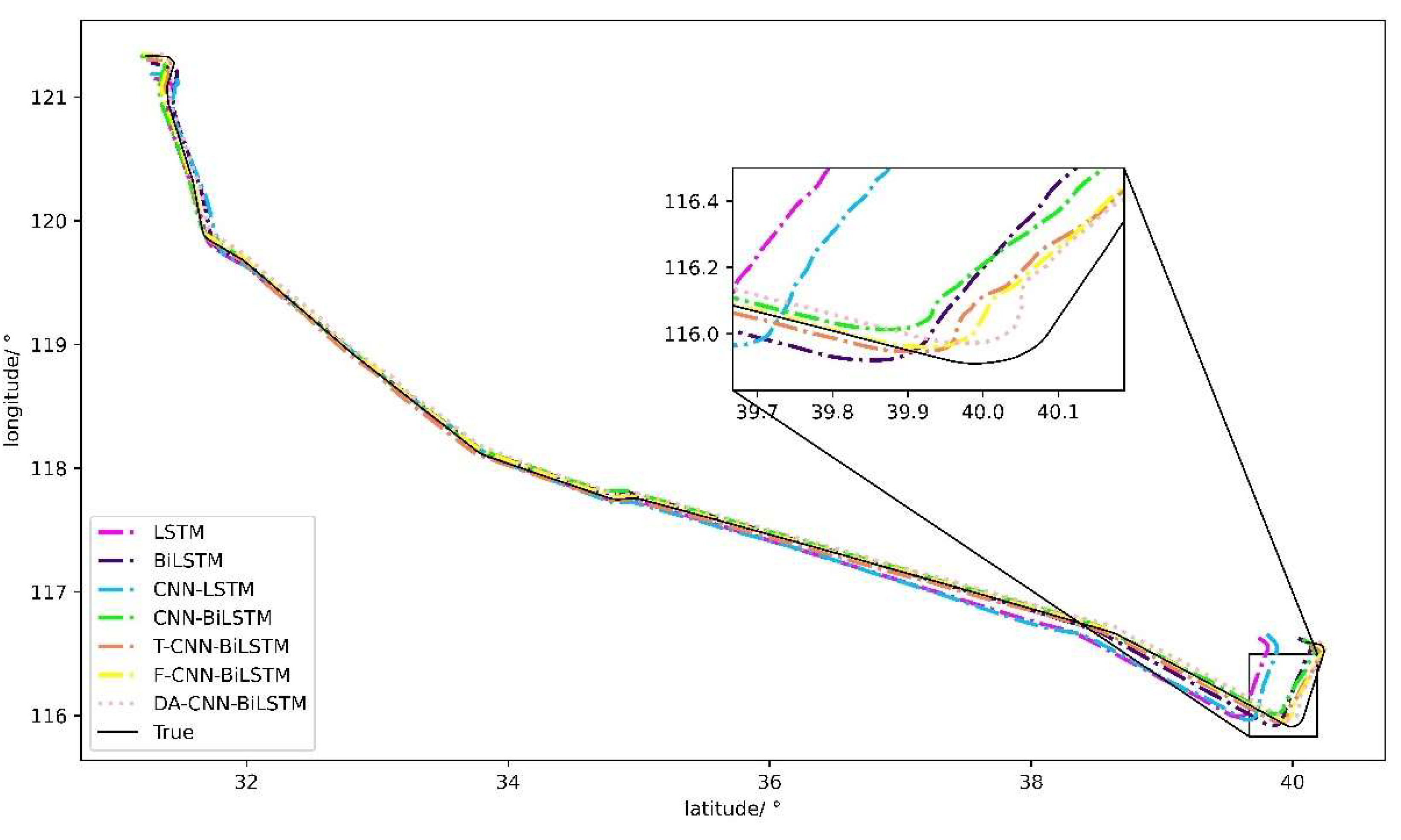
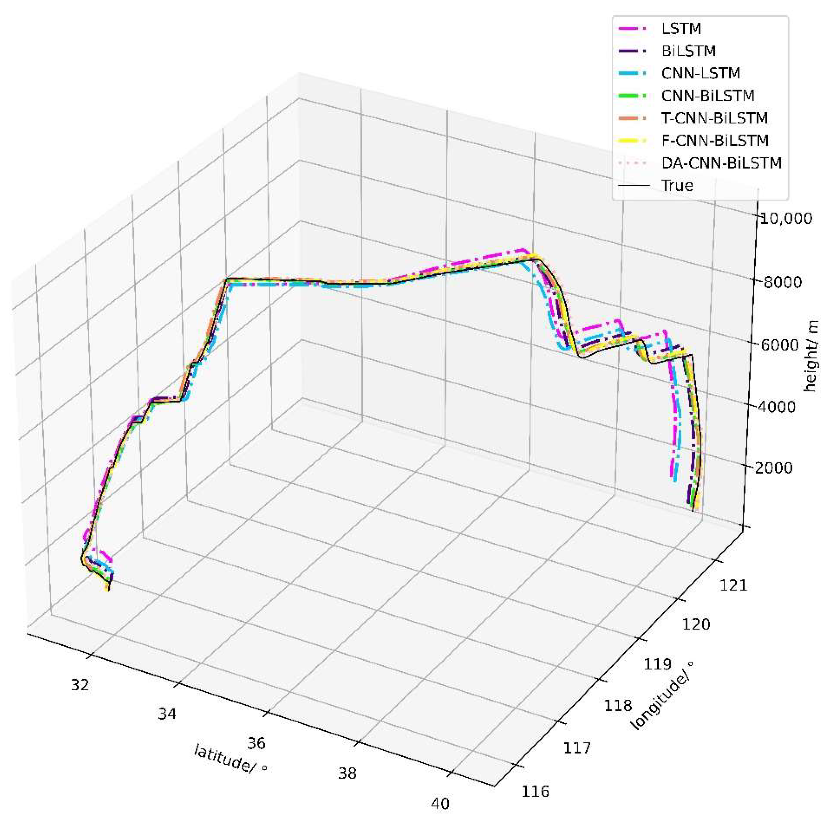
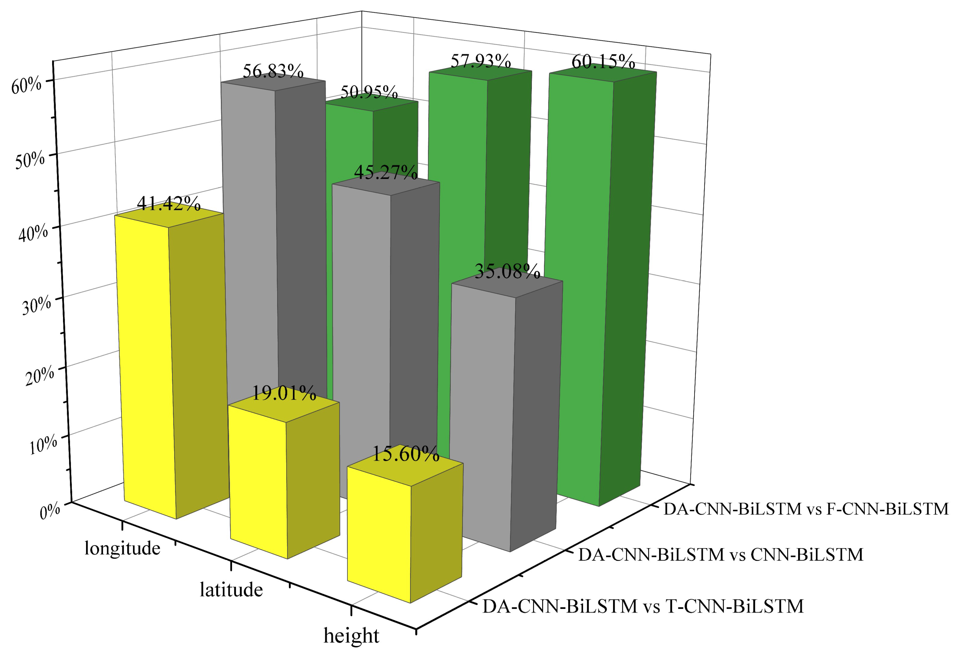
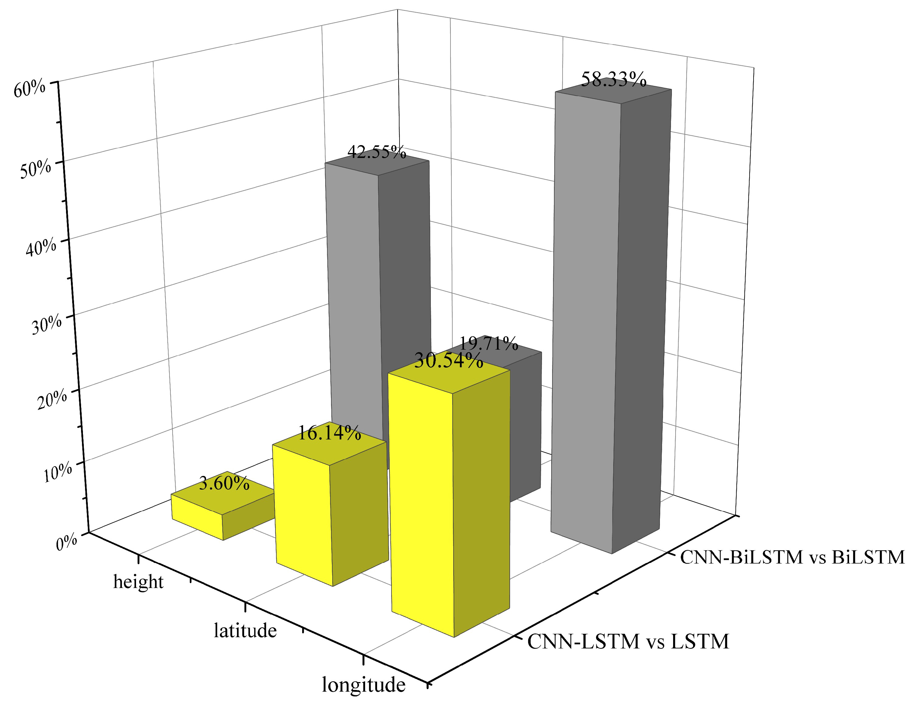
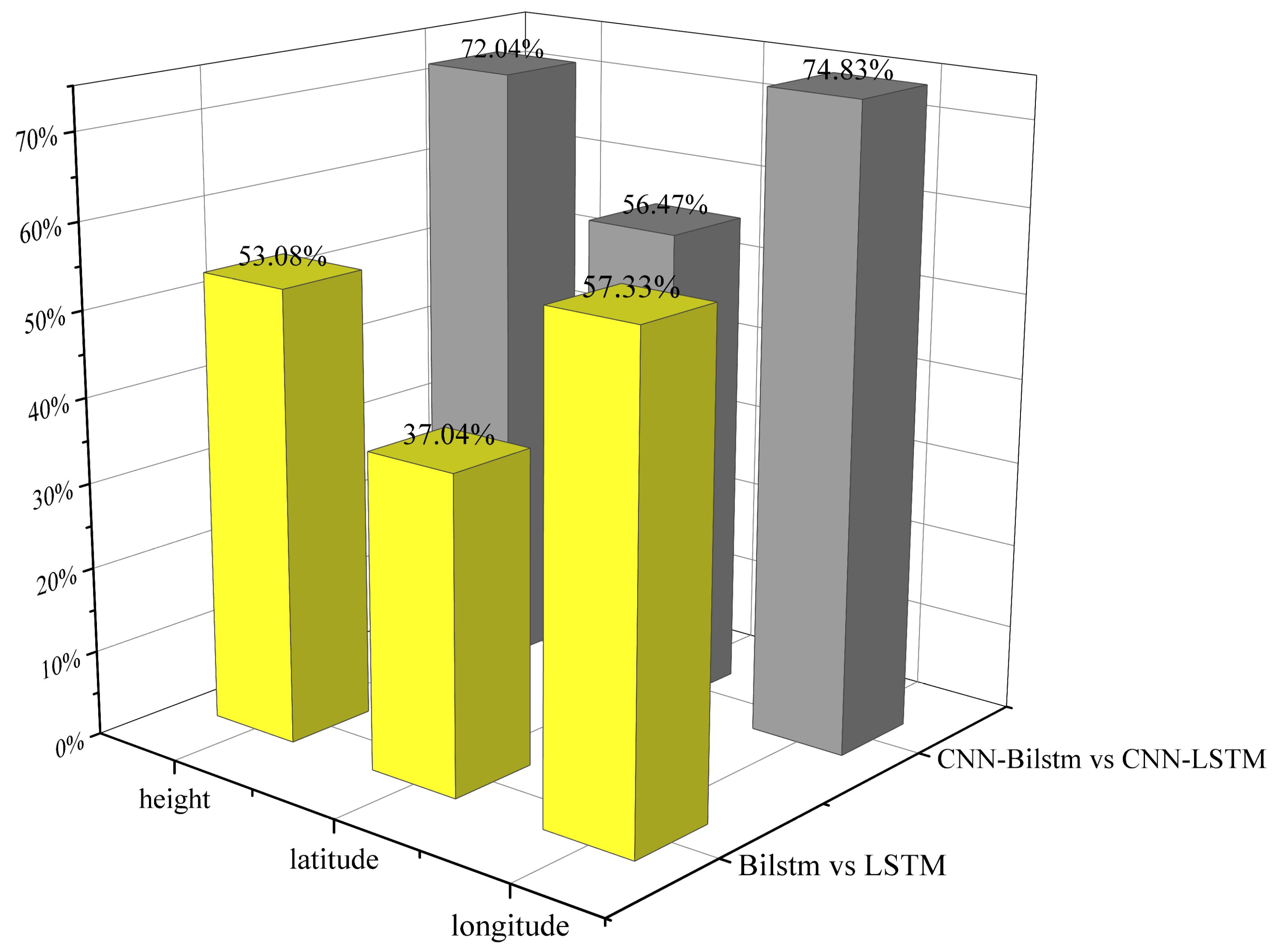
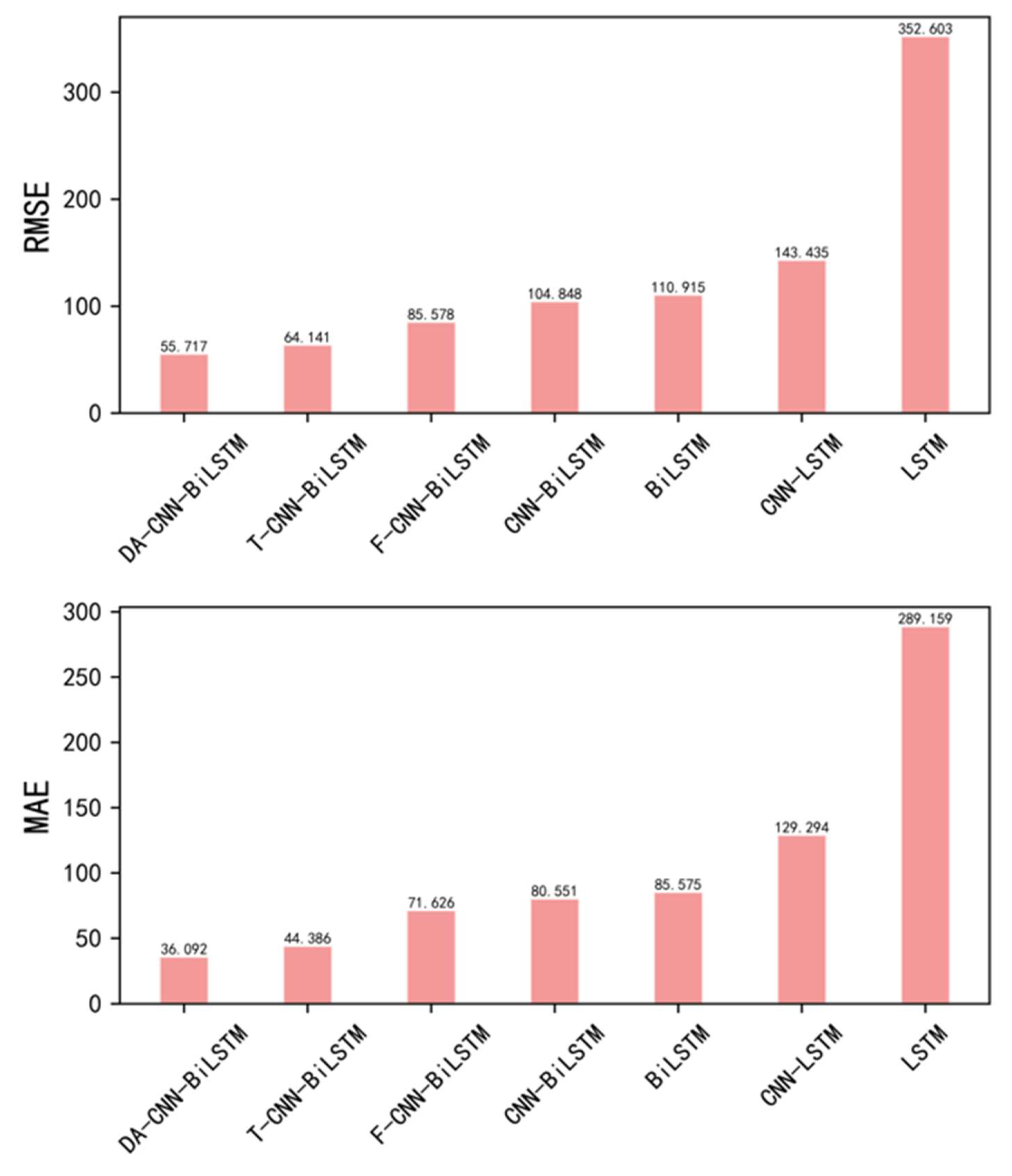
- The performances of the different models in trajectory prediction were systematically investigated. Three sets of comparisons were made. Specifically, the role of introducing CNN in extracting spatial features of the trajectory data was investigated. The bi-directional temporal feature extraction capability of the BiLSTM was verified by comparing BiLSTM to LSTM. In addition, a comparative analysis of temporal attention (T-CNN-BiLSTM), feature attention (F-CNN-BiLSTM), and dual attention (DA-CNN-BiLSTM) was conducted to investigate the impact of feature attention and temporal attention mechanisms on the prediction accuracy.
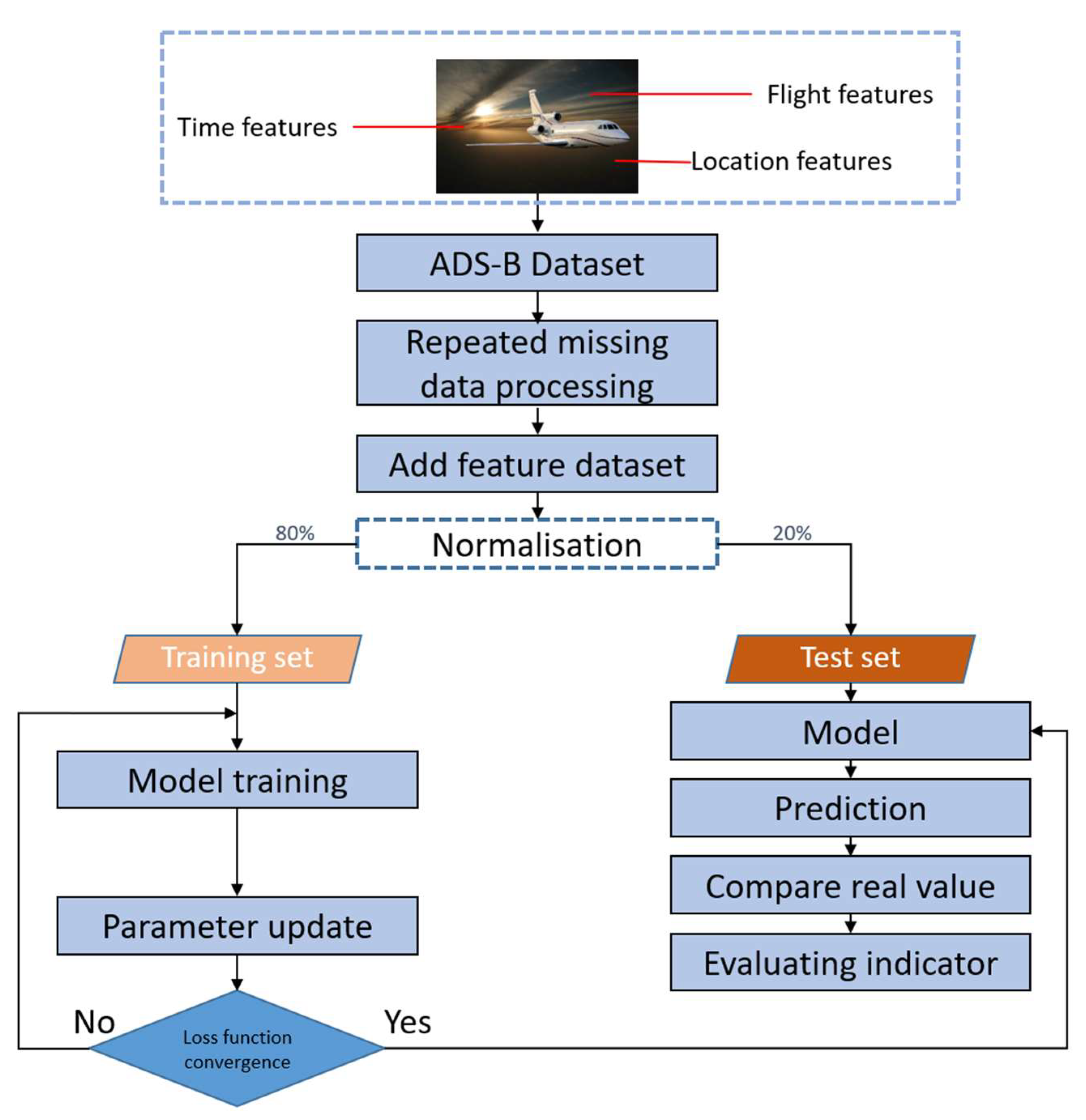
2. ADS-B Data Analysis and Processing
2.1. ADS-B Properties
2.2. Preprocessing of the ADS-B Trajectory
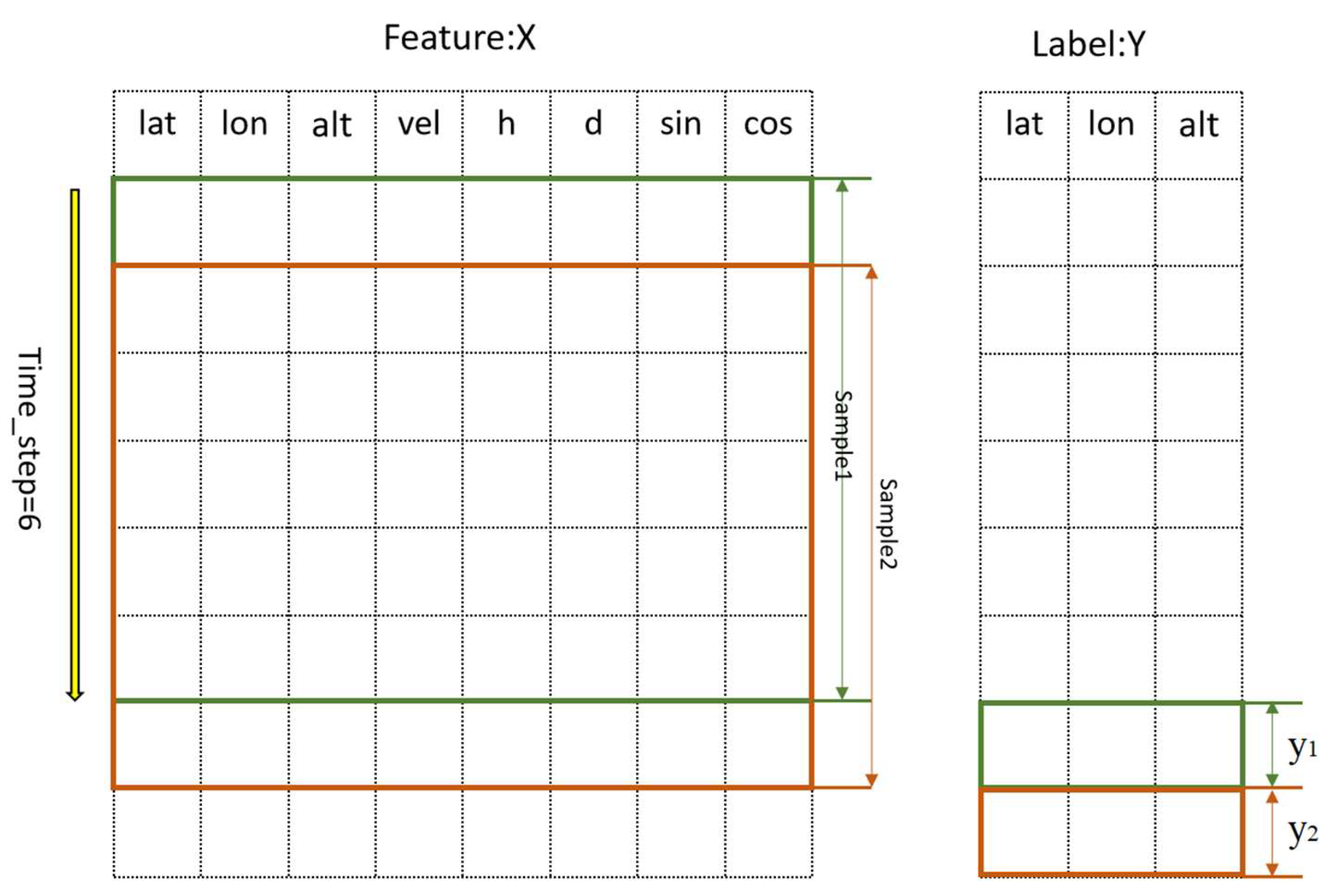
2.3. Sample Construction
3. Methods
3.1. CNN Network
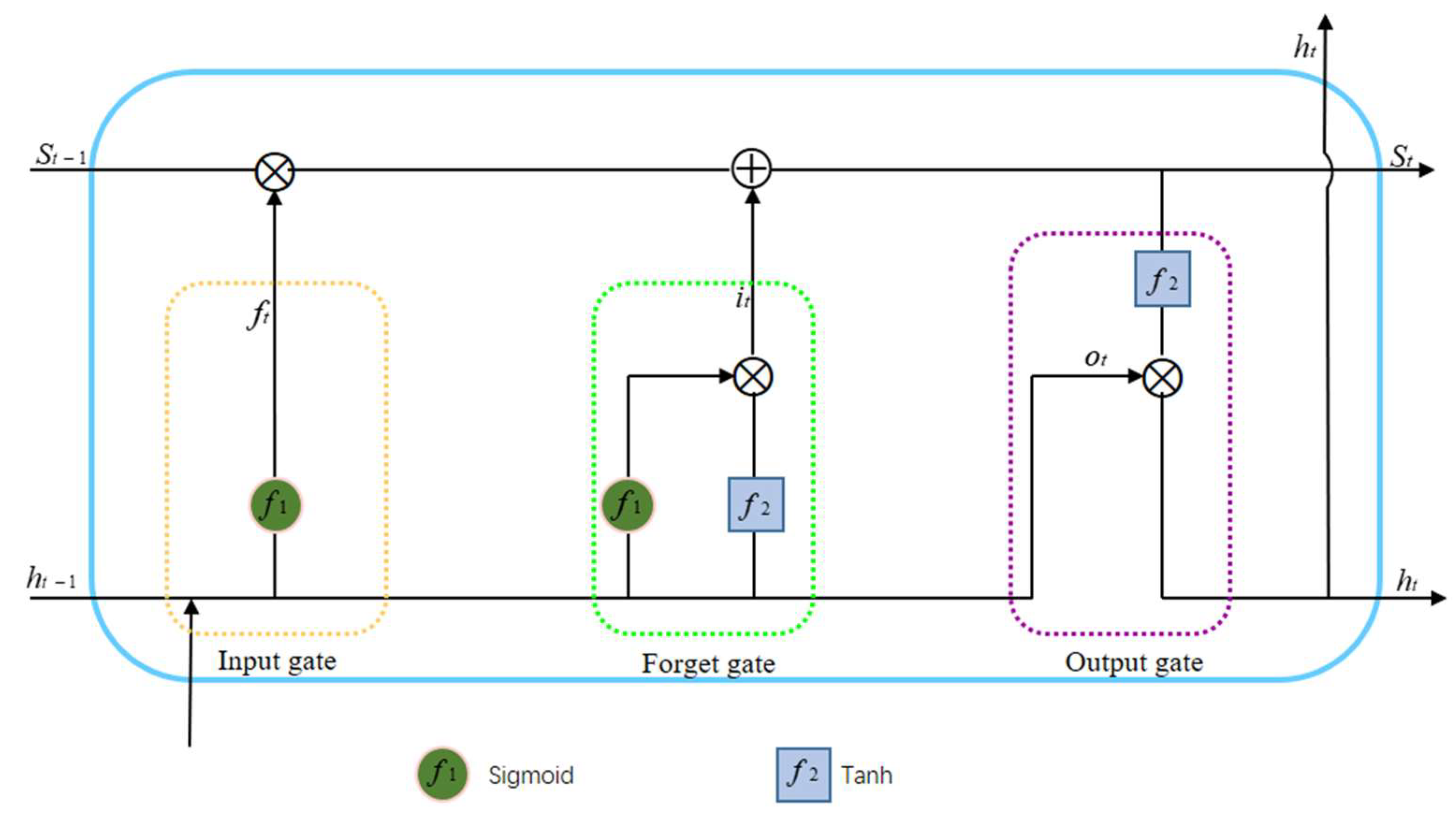
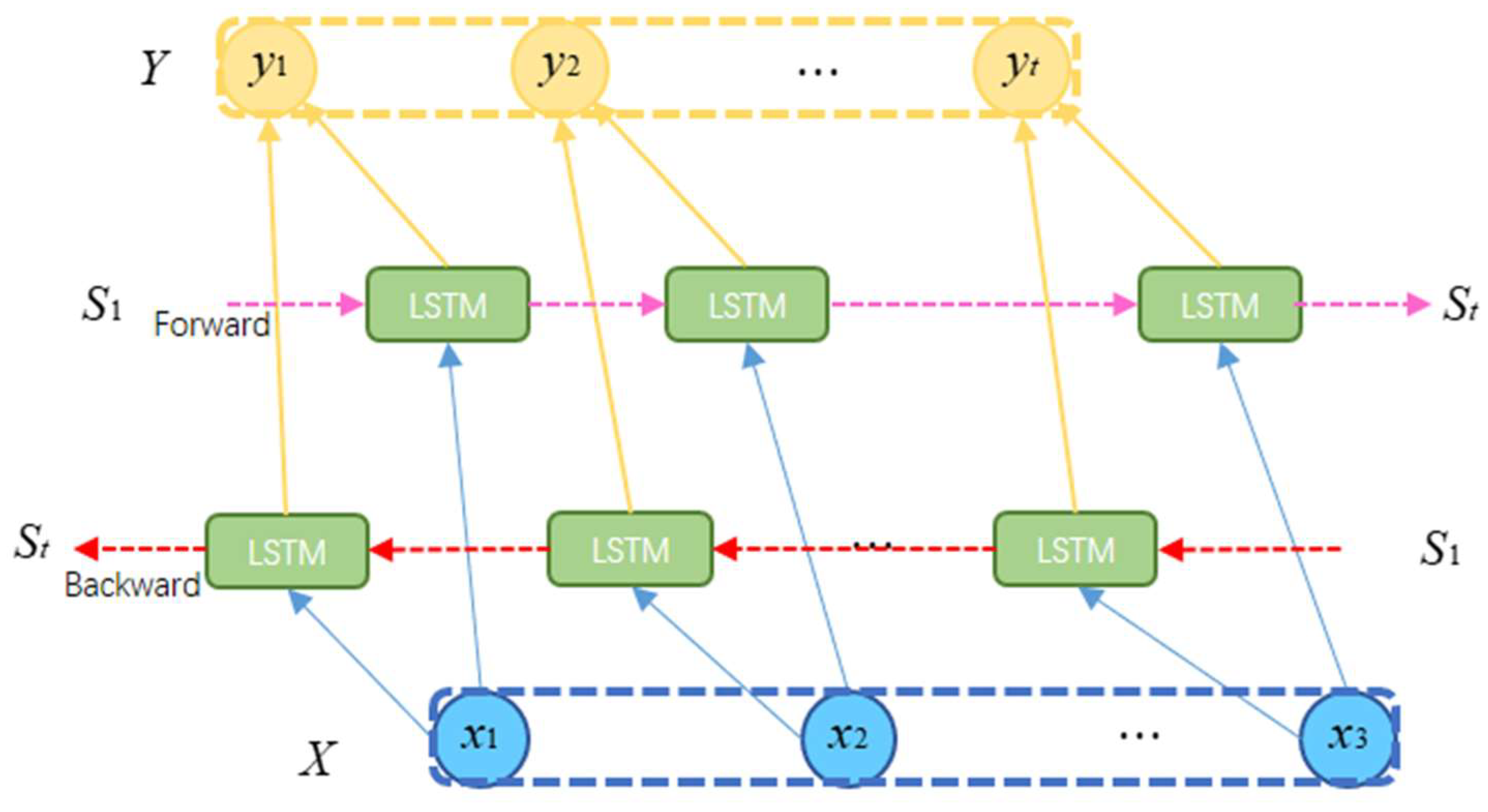
3.2. BiLSTM Network
3.3. Attention Mechanism
3.4. DA-CNN-BiLSTM Model
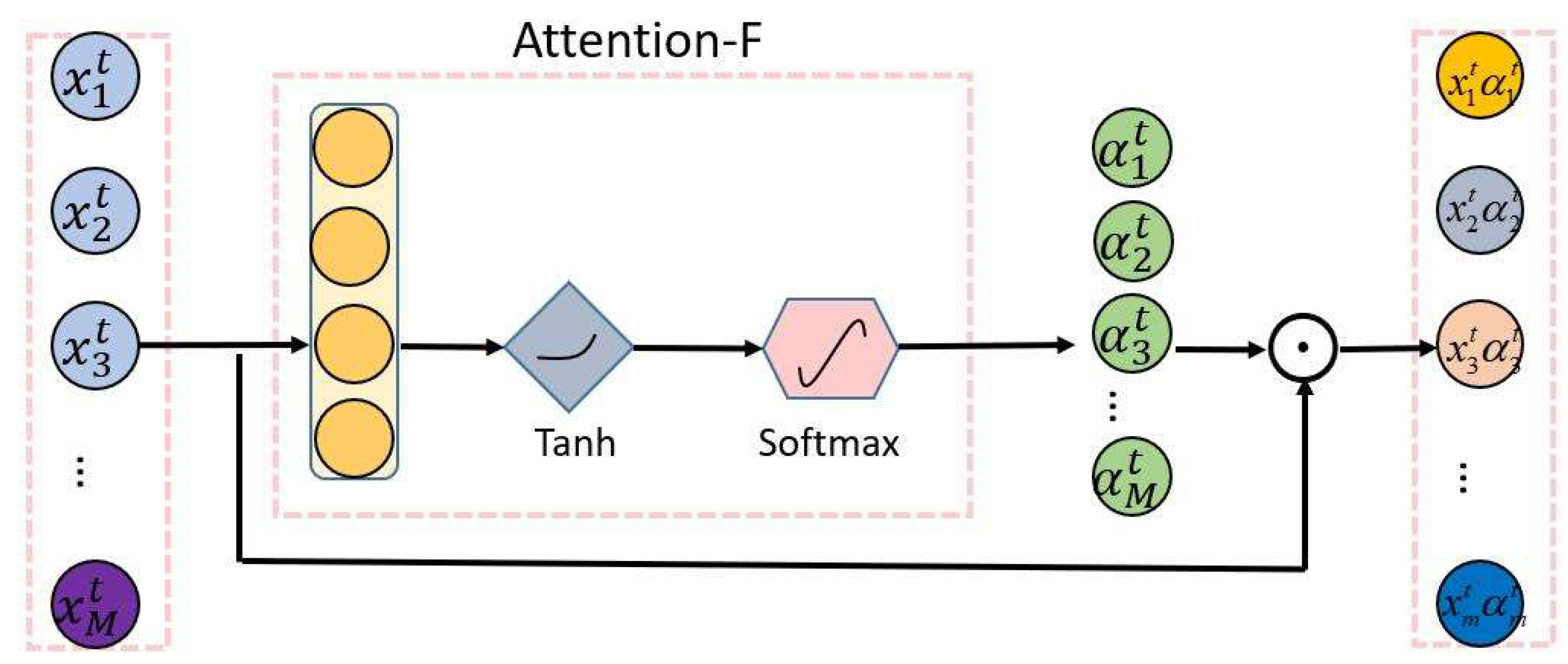
3.4.1. Feature Attention
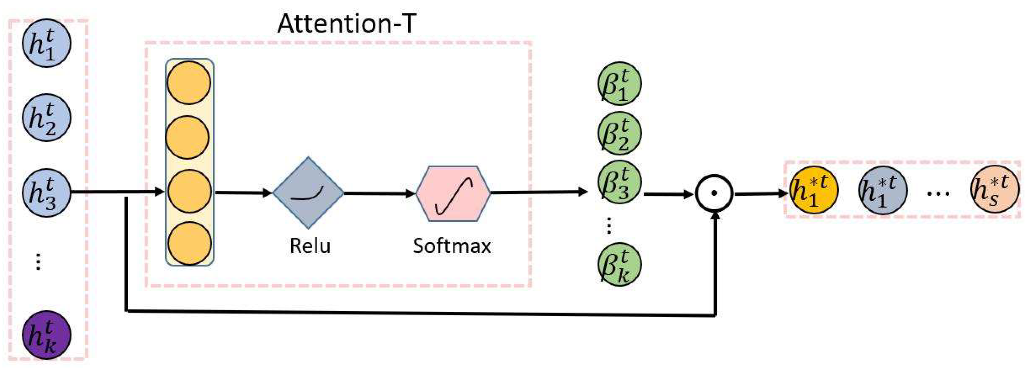
3.4.2. Temporal Attention
3.4.3. DA-CNN-BiLSTM Trajectory Prediction Model
4. Case Analysis
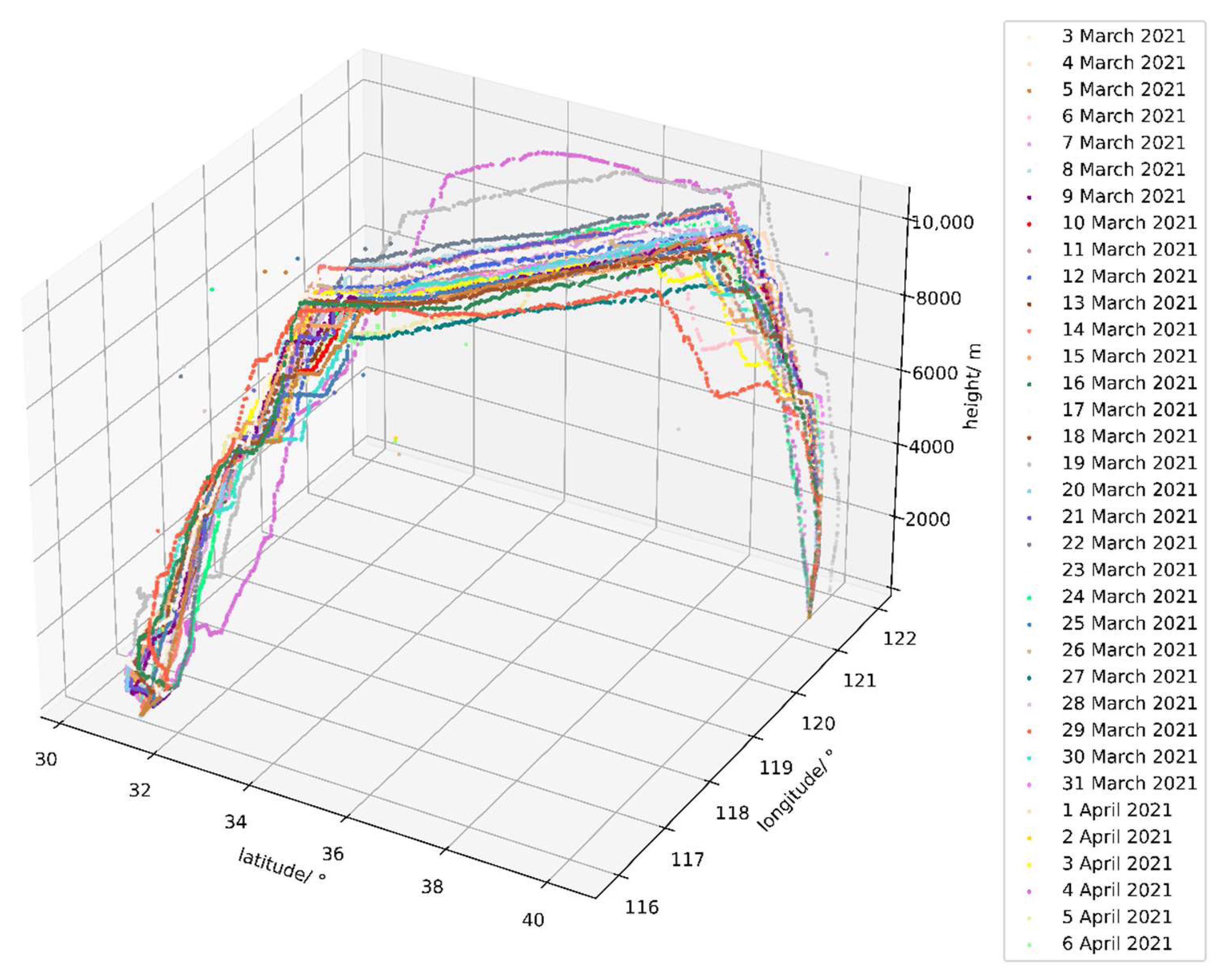
4.1. Experimental Datasets
4.2. Evaluation Index
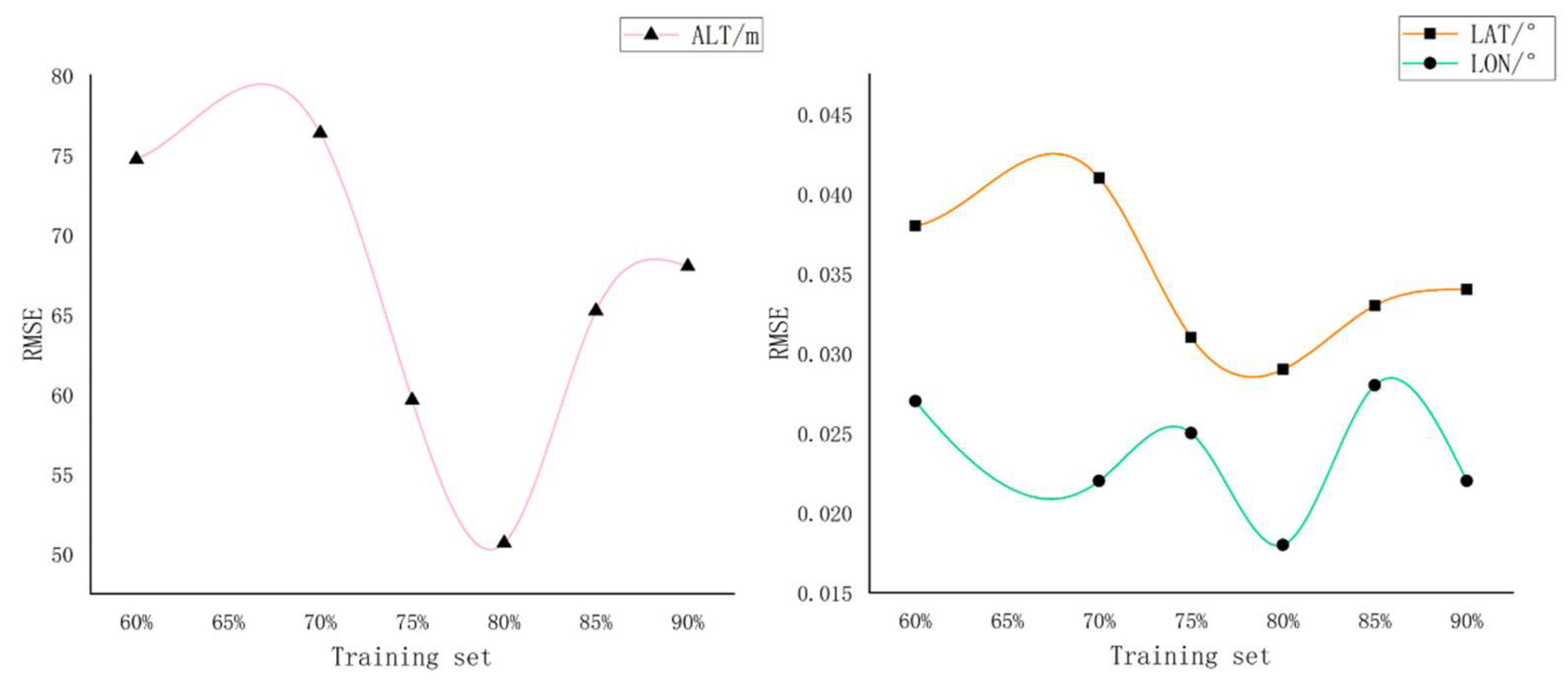
4.3. Calibration of the Model Parameter
- (1)
- Optimisation parameters: According to the DA-CNN-BiLSTM prediction model, the neural network parameters to be optimised include the number, size, and stride of the convolutional kernels of the two-layer CNN, the number of neurons of the two-layer BiLSTM, as well as the dropout rate and learning rate.
- (2)
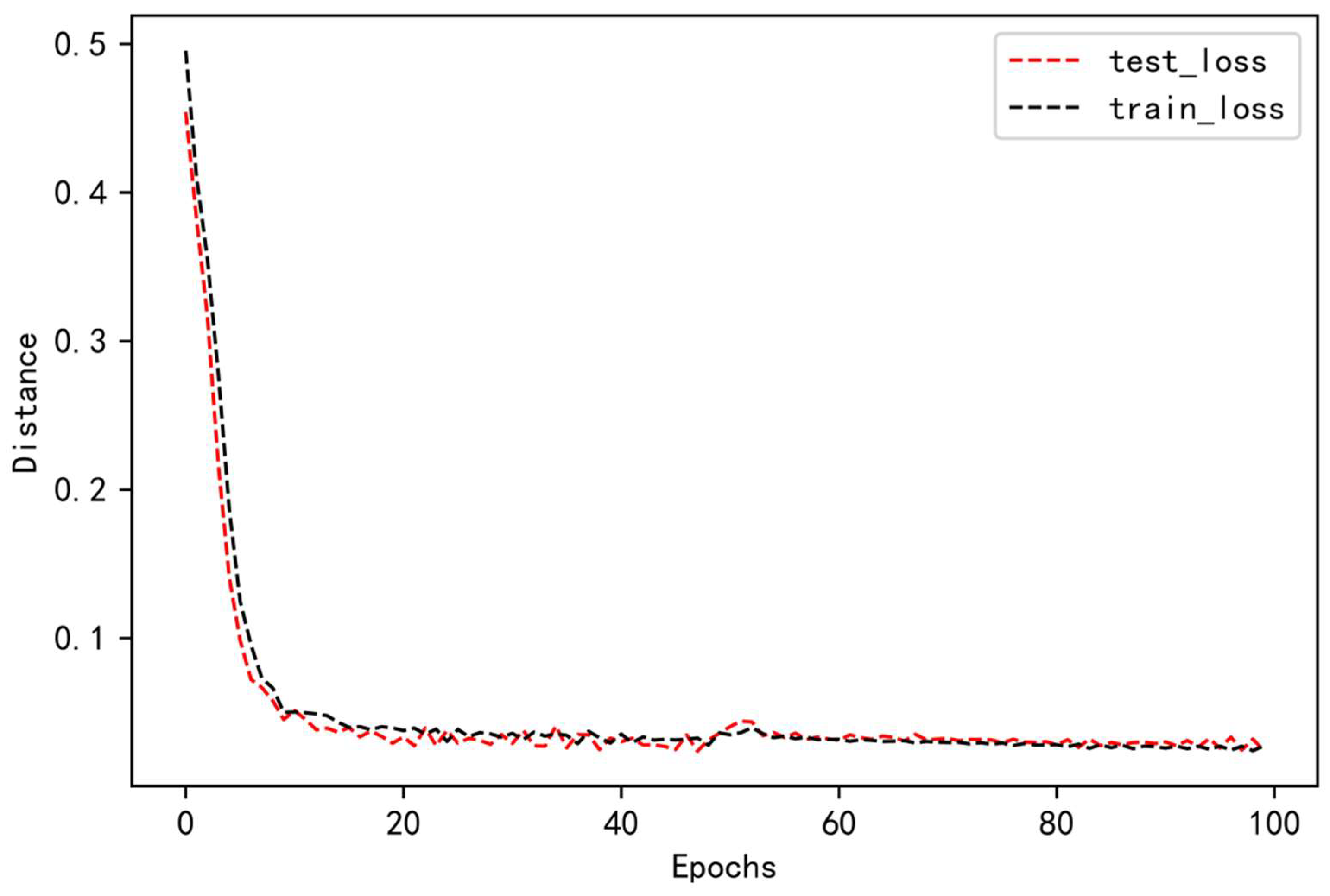
- Objective function: The function Euclidean distance is as shown in Equation (26).
- (3)
- Range of parameters: , , , , , , , , ,
- (4)
- GA parameters: Population size = 20, DNA length = 40, mutation rate = 0.01, max iteration = 5.
4.4. Experiments and Comparison
4.4.1. Experimental Results
4.4.2. Comparative Analysis
4.5. Further Research
5. Conclusions and Discussion
Author Contributions
Funding
Institutional Review Board Statement
Informed Consent Statement
Data Availability Statement
Conflicts of Interest
References
- Mondoloni, S.; Rozen, N. Aircraft Trajectory Prediction and Synchronization for Air Traffic Management Applications. Prog. Aerosp. Sci. 2020, 119, 100640. [Google Scholar] [CrossRef]
- Sahadevan, D.; Ponnusamy, P.; Gopi, V.P.; Nelli, M.K. Ground-based 4d trajectory prediction using bi-directional LSTM networks. Appl. Intell. 2022, 32, 1–18. [Google Scholar] [CrossRef]
- Rosenow, J.; Fricke, H. Impact of multi-criteria optimized trajectories on European airline efficiency, safety and airspace demand. J. Air Transp. Manag. 2019, 78, 133–143. [Google Scholar] [CrossRef]
- Li, X.; Yan, H.; Zhang, Y. Optimization of Multisource Dynamic Model in TBO. Math. Probl. Eng. 2022, 2022, 3755574. [Google Scholar] [CrossRef]
- Zeng, W.; Chu, X.; Xu, Z.; Liu, Y.; Quan, Z. Aircraft 4D Trajectory Prediction in Civil Aviation: A Review. Aerospace 2022, 9, 91. [Google Scholar] [CrossRef]
- Hashemi, S.M.; Botez, R.M.; Grigorie, T.L. New Reliability Studies of Data-Driven Aircraft Trajectory Prediction. Aerospace 2020, 7, 145. [Google Scholar] [CrossRef]
- Zhang, J.; Ge, T.; Chen, Q.; Wang, F. 4D Trajectory Prediction and Uncertainty Analysis for Departure Aircraft. J. Southwest Jiaotong Univ. 2016, 51, 800–806. [Google Scholar]
- He, D.Y. Research on Aircraft Trajectory Planning Based on Centralised Flight Plan Processing. Master’s Thesis, Civil Aviation Flight Academy of China, Chengdu, China, 2020. [Google Scholar]
- Kang, N.; Han, X.; Hu, Y.; Wei, Z. Departure aircraft altitude profile prediction based on aircraft mass estimation strategy. J. Civ. Aviat. Univ. China 2019, 37, 11–16. [Google Scholar]
- Lee, J.; Lee, S.; Hwang, I. Hybrid System Modeling and Estimation for Arrival Time Prediction in Terminal Airspace. J. Guid. Control. Dyn. 2016, 39, 903–910. [Google Scholar] [CrossRef]
- Chen, M.; Fu, J. Flight Track Prediction Method Based on Unscented Kalman Filter. Comput. Simul. 2021, 38, 27–30+36. [Google Scholar]
- Lv, B.; Wang, C. Application of improved extended Kalman filtering in aircraft 4D trajectory prediction algorithm. J. Comput. Appl. 2021, 277–282. [Google Scholar]
- Zhou, J.; Zhang, H.; Lyu, W.; Wan, J.; Zhang, J.; Song, W. Hybrid 4-Dimensional Trajectory Prediction Model, Based on the Reconstruction of Prediction Time Span for Aircraft en Route. Sustainability 2022, 14, 3862. [Google Scholar] [CrossRef]
- Tang, X.; Zheng, P. IMM aircraft short-term track extrapolation based on geodetic coordinate system. Syst. Eng. Electron. 2022, 44, 2293–2301. [Google Scholar]
- Sighencea, B.I.; Stanciu, R.I.; Caleanu, C.D. A Review of Deep Learning-Based Methods for Pedestrian Trajectory Prediction. Sensors 2021, 21, 7543. [Google Scholar] [CrossRef] [PubMed]
- Zhang, Z.; Ni, G.; Xu, Y. Ship Trajectory Prediction Based on LSTM Neural Network. In Proceedings of 2020 IEEE 5th Information Technology and Mechatronics Engineering Conference (itoec 2020), Chongqing, China, 12–14 June 2020; Xu, B., Mou, K., Eds.; IEEE: New York, NY, USA, 2020; pp. 1356–1364. [Google Scholar]
- Karimzadeh, M.; Aebi, R.; de Souza, A.M.; Zhao, Z.; Braun, T.; Sargento, S.; Villas, L. Reinforcement Learning-Designed LSTM for Trajectory and Traffic Flow Prediction. In Proceedings of the 2021 IEEE Wireless Communications and Networking Conference (WCNC), Nanjing, China, 29 March 2021; pp. 1–6. [Google Scholar]
- Han, P.; Wang, W.; Shi, Q.; Yue, J. A Combined Online-Learning Model with K-Means Clustering and GRU Neural Networks for Trajectory Prediction. Ad Hoc Netw. 2021, 117, 102476. [Google Scholar] [CrossRef]
- Madar, S.; Puranik, T.G.; Mavris, D.N. Application of Trajectory Clustering for Aircraft Conflict Detection. In Proceedings of the 2021 IEEE/AIAA 40th Digital Avionics Systems Conference (DASC), San Antonio, TX, USA, 3 October 2021; pp. 1–9. [Google Scholar]
- Yin, Y.; Tong, M. Application of GRIB Data for 4D Trajectory Prediction. In Proceedings of the Artificial Intelligence in China; Liang, Q., Wang, W., Mu, J., Liu, X., Na, Z., Chen, B., Eds.; Springer: Singapore, 2020; pp. 422–430. [Google Scholar]
- Pang, Y.; Xu, N.; Liu, Y. Aircraft Trajectory Prediction Using LSTM Neural Network with Embedded Convolutional Layer. Annu. Conf. PHM Soc. 2019, 11, 11. [Google Scholar] [CrossRef]
- Liu, L.; Zhai, L.; Han, Y. Aircraft trajectory prediction based on conv LSTM. Comput. Eng. Des. 2022, 43, 1127–1133. [Google Scholar] [CrossRef]
- Shi, Q.; Wang, W.; Han, P. Short-term 4D Trajectory Prediction Algorithm Based on Online-updating LSTM Network. J. Signal Process. 2021, 37, 66–74. [Google Scholar] [CrossRef]
- Zeng, W.; Quan, Z.; Zhao, Z.; Xie, C.; Lu, X. A Deep Learning Approach for Aircraft Trajectory Prediction in Terminal Airspace. IEEE Access 2020, 8, 151250–151266. [Google Scholar] [CrossRef]
- Han, P.; Yue, J.; Fang, C.; Shi, Q.; Yang, J. Short-Term 4D Trajectory Prediction Based on LSTM Neural Network. In Proceedings of the Second Target Recognition and Artificial Intelligence Summit Forum; Wang, T., Chai, T., Fan, H., Yu, Q., Eds.; SPIE: Changchun, China, 2020; p. 23. [Google Scholar]
- Shi, Z.; Xu, M.; Pan, Q.; Yan, B.; Zhang, H. LSTM-Based Flight Trajectory Prediction. In Proceedings of the 2018 International Joint Conference on Neural Networks (IJCNN), Rio de Janeiro, Brazil, 8–13 July 2018; pp. 1–8. [Google Scholar]
- Yang, K.; Bi, M.; Liu, Y.; Zhang, Y. LSTM-based deep learning model for civil aircraft position and attitude prediction approach. In Proceedings of the 2019 Chinese Control Conference (CCC), Guangzhou, China, 27–30 July 2019; pp. 8689–8694. [Google Scholar]
- Xu, Z.; Zeng, W.; Chu, X.; Cao, P. Multi-Aircraft Trajectory Collaborative Prediction Based on Social Long Short-Term Memory Network. Aerospace 2021, 8, 115. [Google Scholar] [CrossRef]
- Ma, L.; Tian, S. A Hybrid CNN-LSTM Model for Aircraft 4D Trajectory Prediction. IEEE Access 2020, 8, 134668–134680. [Google Scholar] [CrossRef]
- Hu, D.; Meng, X.; Lu, S.; Xing, L. Parallel LSTM-FCN Model Applied to Vessel Trajectory Prediction. Control Decis. 2022, 37, 1–7. [Google Scholar] [CrossRef]
- Manesh, M.R.; Kaabouch, N. Analysis of Vulnerabilities, Attacks, Countermeasures and Overall Risk of the Automatic Dependent Surveillance-Broadcast (ADS-B) System. Int. J. Crit. Infrastruct. Prot. 2017, 19, 16–31. [Google Scholar] [CrossRef]
- Zhou, F.; Jin, L.; Dong, J. Review of convolutional neural network. Chin. J. Comput. 2017, 40, 1229–1251. [Google Scholar]
- Yu, Y.; Si, X.; Hu, C.; Zhang, J. A review of recurrent neural networks: LSTM cells and network architectures. Neural Comput. 2019, 31, 1235–1270. [Google Scholar] [CrossRef] [PubMed]
- Peng, Y.; Han, Q.; Su, F.; He, X.; Feng, X. Meteorological Satellite Operation Prediction Using a BiLSTM Deep Learning Model. Secur. Commun. Netw. 2021, 2021, 9916461. [Google Scholar] [CrossRef]
- Li, A.; Xiao, F.; Zhang, C.; Fan, C. Attention-based interpretable neural network for building cooling load prediction. Appl. Energy 2021, 299, 117238. [Google Scholar] [CrossRef]
- Meng, Q.; Shang, B.; Liu, Y.; Guo, H.; Zhao, X. Intelligent Vehicles Trajectory Prediction with Spatial and Temporal Attention Mechanism. In Proceedings of the Ifac Papersonline; Elsevier: Amsterdam, The Netherlands, 2021; Volume 54, pp. 454–459. [Google Scholar]
- Lin, Z.; Cheng, L.; Huang, G. Electricity Consumption Prediction Based on LSTM with Attention Mechanism. IEEJ Trans. Electr. Electron. Eng. 2020, 15, 556–562. [Google Scholar] [CrossRef]
- He, X.; He, Z.; Song, J.; Liu, Z.; Jiang, Y.-G.; Chua, T.-S. Nais: Neural attentive item similarity model for recommendation. IEEE Trans. Knowl. Data Eng. 2018, 30, 2354–2366. [Google Scholar] [CrossRef] [Green Version]


| Feature | Trajectory Point |
|---|---|
| Time | 4 March 20211 3: 38: 22 |
| Anum | B5372 |
| Forum | HU7603 |
| Longitude/(°) | 116.26586 |
| Latitude/(°) | 39.37152 |
| Altitude/(m) | 8610.61 |
| Velocity/(km/h) | 890.81 |
| Angle/(°) | 156 |
| Distance/(m) | 1,016,975.48 |
| −0.333 | |
| 0.943 |
| Model | |||||||||
|---|---|---|---|---|---|---|---|---|---|
| DA-CNN-BiLSTM | CNN | Convolution | Filter = 50; Kernel size = 3; Stride = 1; | Epochs = 100; Batch size = 256; Optimiser = ‘Adam’; Learning rate = 0.002591 | |||||
| Max-pooling | Kernel size = 2; Stride = 1; | ||||||||
| Convolution | Filter = 50; Kernel size = 2; Stride = 1; | ||||||||
| Max-pooling | Kernel size = 2; Stride = 1; | ||||||||
| F-Attention-Layer | |||||||||
| BiLSTM | Units1 | Units80 | |||||||
| Dropout | 0.2493 | ||||||||
| Units2 | Units90 | ||||||||
| Dropout | 0.2493 | ||||||||
| T-Attention-Layer | |||||||||
| Output | Dense | 3 | |||||||
| RMSE | |||||||
|---|---|---|---|---|---|---|---|
| Hybrid Model | Single Model | ||||||
| DA-CNN-BiLSTM | T-CNN-BiLSTM | F-CNN-BiLSTM | CNN-BiLSTM | CNN-LSTM | BiLSTM | LSTM | |
| Alt/(m) | 50.68 | 60.05 | 127.17 | 78.07 | 310.13 | 189.64 | 446.52 |
| Lat/(°) | 0.029 | 0.036 | 0.069 | 0.043 | 0.189 | 0.092 | 0.196 |
| Lon/(°) | 0.018 | 0.031 | 0.038 | 0.053 | 0.098 | 0.053 | 0.084 |
| MAE | |||||||
| Hybrid Model | Single Model | ||||||
| DA-CNN-BiLSTM | T-CNN-BiLSTM | F-CNN-BiLSTM | CNN-BiLSTM | CNN-LSTM | BiLSTM | LSTM | |
| Alt/(m) | 32.37 | 38.35 | 116.06 | 60.27 | 219.16 | 151.13 | 329.12 |
| Lat/(°) | 0.022 | 0.027 | 0.063 | 0.033 | 0.158 | 0.081 | 0.128 |
| Lon/(°) | 0.014 | 0.025 | 0.033 | 0.048 | 0.08 | 0.045 | 0.059 |
| Details | |||||
|---|---|---|---|---|---|
| 1st set comparison | DA-CNN-BiLSTM vs. T-CNN-BiLSTM | DA-CNN-BiLSTM vs. F-CNN-BiLSTM | DA-CNN-BiLSTM vs. CNN-BiLSTM | ||
| 2nd set comparison | CNN-LSTM vs. LSTM | CNN-BiLSTM vs. BiLSTM | |||
| 3rd set comparison | BiLSTM vs. LSTM | CNN-BiLSTM vs. CNN-BiLSTM | |||
Publisher’s Note: MDPI stays neutral with regard to jurisdictional claims in published maps and institutional affiliations. |
© 2022 by the authors. Licensee MDPI, Basel, Switzerland. This article is an open access article distributed under the terms and conditions of the Creative Commons Attribution (CC BY) license (https://creativecommons.org/licenses/by/4.0/).
Share and Cite
Ding, W.; Huang, J.; Shang, G.; Wang, X.; Li, B.; Li, Y.; Liu, H. Short-Term Trajectory Prediction Based on Hyperparametric Optimisation and a Dual Attention Mechanism. Aerospace 2022, 9, 464. https://doi.org/10.3390/aerospace9080464
Ding W, Huang J, Shang G, Wang X, Li B, Li Y, Liu H. Short-Term Trajectory Prediction Based on Hyperparametric Optimisation and a Dual Attention Mechanism. Aerospace. 2022; 9(8):464. https://doi.org/10.3390/aerospace9080464
Chicago/Turabian StyleDing, Weijie, Jin Huang, Guanyu Shang, Xuexuan Wang, Baoqiang Li, Yunfei Li, and Hourong Liu. 2022. "Short-Term Trajectory Prediction Based on Hyperparametric Optimisation and a Dual Attention Mechanism" Aerospace 9, no. 8: 464. https://doi.org/10.3390/aerospace9080464