Numerical Study on the Non-Oscillatory Unstarted Flow in a Scramjet Inlet-Isolator Model

Abstract

For successful scramjet engine operations, it is important to understand the mechanism of the inlet unstart phenomenon. Among various unstarted flow patterns in hypersonic inlets, the mechanism of low-amplitude oscillatory unstarted flow is still unclear. Therefore, in the present study, the flow characteristics of non-oscillatory unstarted flow in a scramjet inlet-isolator model are studied by using numerical analysis with the RANS-based OpenFOAM solver. In the numerical results, the amplitude of pressure oscillation and the average pressure near the model outlet are in good agreement with experimental results. In the detailed analysis of the results, it is found that the incoming flow within the boundary layers repeatedly changes direction due to the flow blockage at the end of the model. In these direction-changing processes, recirculation zones near the walls irregularly influence the choked flow zones at the rear part of the model. These irregular behaviors result in non-oscillatory unstarted flow. Additionally, the main differences between the high-amplitude oscillatory unstarted flow and non-oscillatory unstarted flow are addressed.

1. Introduction

The inlet buzz phenomenon was first observed by Oswatitsch as a pressure oscillation phenomenon that occurs when an inlet unstart occurs [1]. The inlet buzz phenomenon reduces or blocks the flow rate into the inlet and can damage the internal structure due to severe pressure oscillation. Therefore, the prevention, prediction, and management of inlet unstart are important issues. To this end, it is essential to determine the inlet unstart flow pattern and unstart mechanism.

Ferri and Nucci conducted experimental studies on the causes and basic mechanisms of supersonic inlet buzz [2]. As a result of the study, they found that the supersonic inlet buzz was an acoustic resonance phenomenon caused by the shear layer of the cowl lip. Likewise, Dailey conducted an experimental study to determine the occurrence mechanism of the supersonic inlet buzz phenomenon [3]. According to Dailey’s experiment, another cause of the supersonic inlet buzz phenomenon was shock-induced flow separation on the external compression surface.

After that, a study on the supersonic inlet buzz was conducted by Fisher et al. and Trapier et al. [4,5,6]. Fisher et al. conducted an experimental study on the supersonic inlet buzz phenomenon by changing the throttling ratio in Mach 2 flow [4]. In their results, two pressure oscillation patterns with similar frequencies and different amplitudes were found, summarized as little buzz and big buzz. Furthermore, the little buzz was caused by the shear layer of the cowl lip (Ferri criterion), and the big buzz was caused by the separation bubble on the compression surface (Dailey criterion). Trapier et al. conducted experimental and numerical studies on the supersonic inlet buzz [5,6]. In the experimental results, pressure oscillation patterns corresponding to a little buzz and a big buzz were observed. Similar to Fisher et al., they confirmed that the cause of the little buzz was related to the Ferri criterion and that the big buzz was related to the Dailey criterion. In addition, the pressure oscillation of the little buzz was reduced by a bleeding device. In the numerical study, the experimental model was simulated using DDES (delayed detached-eddy simulation). The numerical results showed that all the features of the buzz phenomenon matched well with their experiments.

As described above, the flow patterns and mechanisms for supersonic inlet buzzes have been somewhat clarified by many studies. However, as Curran and Murthy pointed out, the unstart flow patterns of the supersonic inlet and the hypersonic inlet are different [7]. Unlike the supersonic inlet, the hypersonic inlet has a supersonic area even after the final shock wave. Due to this difference, the causes of the unstart pattern of the hypersonic inlet vary, and the flow patterns are different for each cause [8]. Therefore, it is difficult to directly apply the research achievements on supersonic inlet buzz to hypersonic inlet buzz.

As a result, many researchers have conducted studies to identify the unstart flow patterns and mechanisms of hypersonic inlets [9,10,11,12,13,14,15]. Tan and Guo conducted an experimental study on the hypersonic inlet unstart phenomenon using a plug at the rear of the inlet model [9]. Their experimental results showed changes in the external shock wave structure and inlet wall pressure. However, the internal flow patterns of the buzz cycle were not identified, and the conclusion was inferred based on the changes in the wall pressure distribution.

Tan et al. conducted an experimental study to identify the unstart flow pattern and buzz frequency of the hypersonic inlet [10]. To simulate the back pressure, a plug was located at the rear of the inlet model. In the results, the pressure oscillation patterns were classified into little buzz and big buzz, but they were different from the little buzz and the big buzz of the supersonic inlet. Furthermore, they found that the oscillation mechanism of the supersonic inlet buzz based on the acoustic wave feedback loop was not suitable for the hypersonic inlet buzz. Therefore, flow spillage was considered a disturbing source, and a new oscillation mechanism for hypersonic inlet buzz was proposed based on a feedback loop suitable for the hypersonic inlet. Using this new feedback loop, the base frequency of the hypersonic inlet buzz was predicted, and it matched well with their experimental results.

However, in addition to little buzz and big buzz, there are other types of inlet unstart patterns in hypersonic inlets [8]. Wagner conducted an experimental study on the hypersonic inlet model at Mach 5 flow [11]. To simulate back pressure, a flap was installed at the rear of the scramjet inlet-isolator model. In the experimental results, three unstart flow patterns were observed. The three patterns were ‘high-amplitude oscillatory unstarted flow’, ‘low-amplitude oscillatory unstarted flow’, and ‘non-oscillatory unstarted flow’.

As such, there are several unstart flow patterns, and the flow characteristics of each pattern are different. With the efforts of many researchers, studies on the flow characteristics and mechanisms of hypersonic inlet unstart have progressed, but there are still components to be identified. Therefore, several follow-up studies have been conducted [12,13,14].

Tan et al. conducted an experimental study on the hypersonic inlet unstart phenomenon in Mach 5 flow using a plug installed at the rear of the inlet model [12]. In the results, the position of the pressure sensor suitable for monitoring the inlet status was presented by analyzing the Schlieren images and the pressure signals. In addition, an overall analysis of each flow pattern was presented based on the behavior of shock structures and separation bubbles, but a detailed analysis of the flow characteristics was not presented. Similarly, Li et al. conducted an experimental study on hypersonic inlet unstart using a plug-installed inlet model [13]. In their results, the study focused on changes in pressure oscillation patterns and shock propagation speeds according to an increase in the throttling ratio rather than the mechanism of the buzz phenomenon. Koo and Raman conducted a numerical study on the inlet unstart phenomenon using LES (large-eddy simulation) by referring to Wagner’s experiment [11,14]. The flow characteristics of the inlet start case were in good agreement with the experimental results, but three types of pressure oscillation patterns of inlet unstart were not found in their results.

Although several follow-up studies have been conducted, explanations of the three different unstart modes found in Wagner’s experiment have rarely been reported. In the authors’ previous study, the numerical results matched well with the pressure oscillation frequency and amplitude of ‘high-amplitude oscillatory unstarted flow’ shown in Wagner’s experiment [15]. In that paper, the flow characteristics and mechanisms of ‘high-amplitude oscillatory unstarted flow’ were explained. Furthermore, the effects of boundary layer types in ‘high-amplitude oscillatory unstarted flow’ were addressed. However, the flow characteristics and mechanisms for the other two inlet unstart modes, ‘non-oscillatory unstarted flow’ and ‘low-amplitude oscillatory unstarted flow’, are still unclear.

Therefore, in the present study, we perform numerical analysis to investigate the flow characteristics of ‘non-oscillatory unstarted flow’ as a follow-up study. The numerical method for the study and the configuration of the test model are introduced in Section 2. In Section 3.1, changes in pressure oscillation patterns according to various flap angles are explained. In Section 3.2 and Section 3.3, the detailed mechanisms of ‘non-oscillatory unstarted flow’ are explained. Finally, in Section 3.4, we address the differences between ‘high-amplitude oscillatory unstarted flow’ and ‘non-oscillatory unstarted flow’.

2. Numerical Method

The open-source CFD (computational fluid dynamics) software OpenFOAM is used to model ‘non-oscillatory unstarted flow’ in the scramjet inlet-isolator model. In a previous study, we validated the overall numerical method through comparison with experimental results [15]. Therefore, in this study, the same numerical method is used. The RANS (Reynolds-averaged Navier-Stokes) equations-based solver rhoCentralFoam, which is suitable for supersonic flow analysis, is employed to solve the Navier–Stokes equations [16,17]. The central-upwind KNP (Kurganov, Noelle, and Petrova) scheme with the van Leer limiter is applied to evaluate the flux at cell faces [17,18]. The boundary layer and recirculation zone are significant factors in the flow characteristics of inlet unstart. To consider these factors, Sutherland’s viscosity model is used as a viscous model, and k-ω SST (shear stress transport) is used as a turbulence model [19,20]. Temperature-dependent thermal properties are taken from the JANAF table [21].

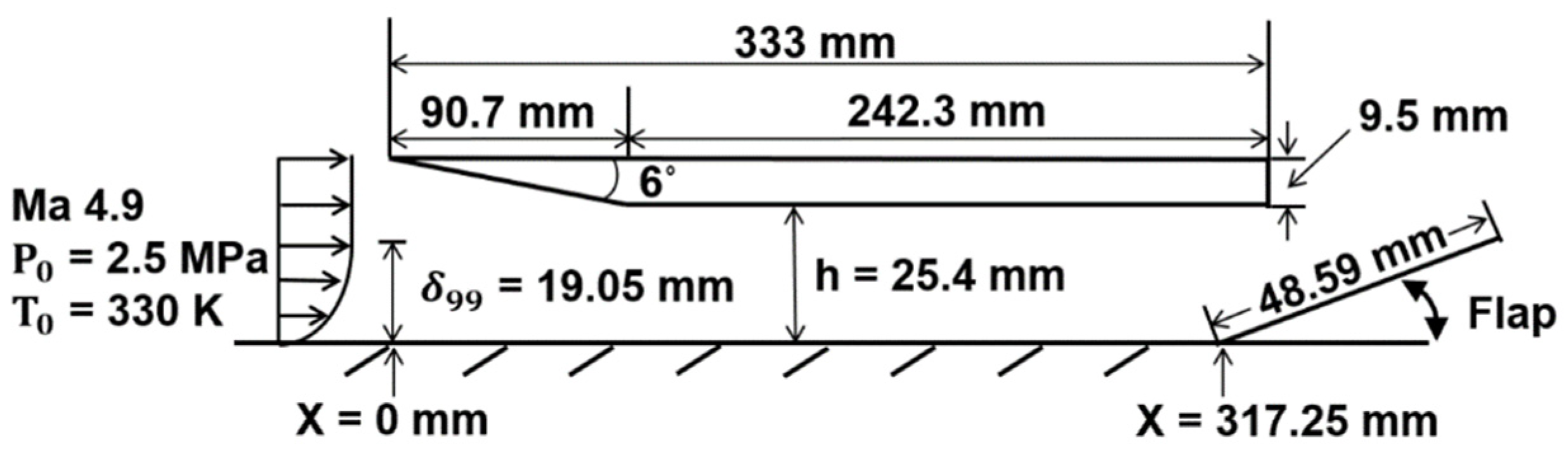
Figure 1 shows the schematic of the scramjet inlet-isolator model. As in a previous study, the configuration and inflow conditions of the scramjet inlet-isolator model are the same as the experimental conditions [11,15]. As shown in the figure, the inflow conditions are a Mach number of 4.9 with a total pressure of 2.5 MPa, and total temperature of 330 K. A 19.05 mm thick turbulent boundary layer is also considered in the inflow. In this case, the boundary layer thickness is 75% of the inlet height. Turbulence boundary layer theory is employed to calculate the velocity profiles of the inflow boundary layer [22,23].

To find the appropriate grid resolution for the problem, a grid independency test is performed.

Table 1. Number of grid cells used in the grid independency test.

	Grid 1	Grid 2	Grid 3	Grid 4
Number of grid cells within the model $(N_x\times N_y)$	$650\times 65$	$380\times 55$	$545\times 64$	$390\times 60$
Model outlet configuration	Flap folded	Flap folded	Flap opened	Flap opened
$\mathrm{Average}{y}^{+}$ on the wall	0.74	0.93	0.93	0.93

shows the number of grid cells used in the test. In the table, Grids 1 and 2 are used for the model with a folded flap and Grids 3 and 4 are used for the model with an opened flap. Since it is important to estimate the development of boundary layers and flow separation in unstarted flows, the average y+ on the wall is set to about 1.0 for all cases. The test results for Grids 1 and 2 are in consistent with each other, and so are those for Grids 3 and 4. Therefore, in the present study, Grid 4 is used for the model with an opened flap. 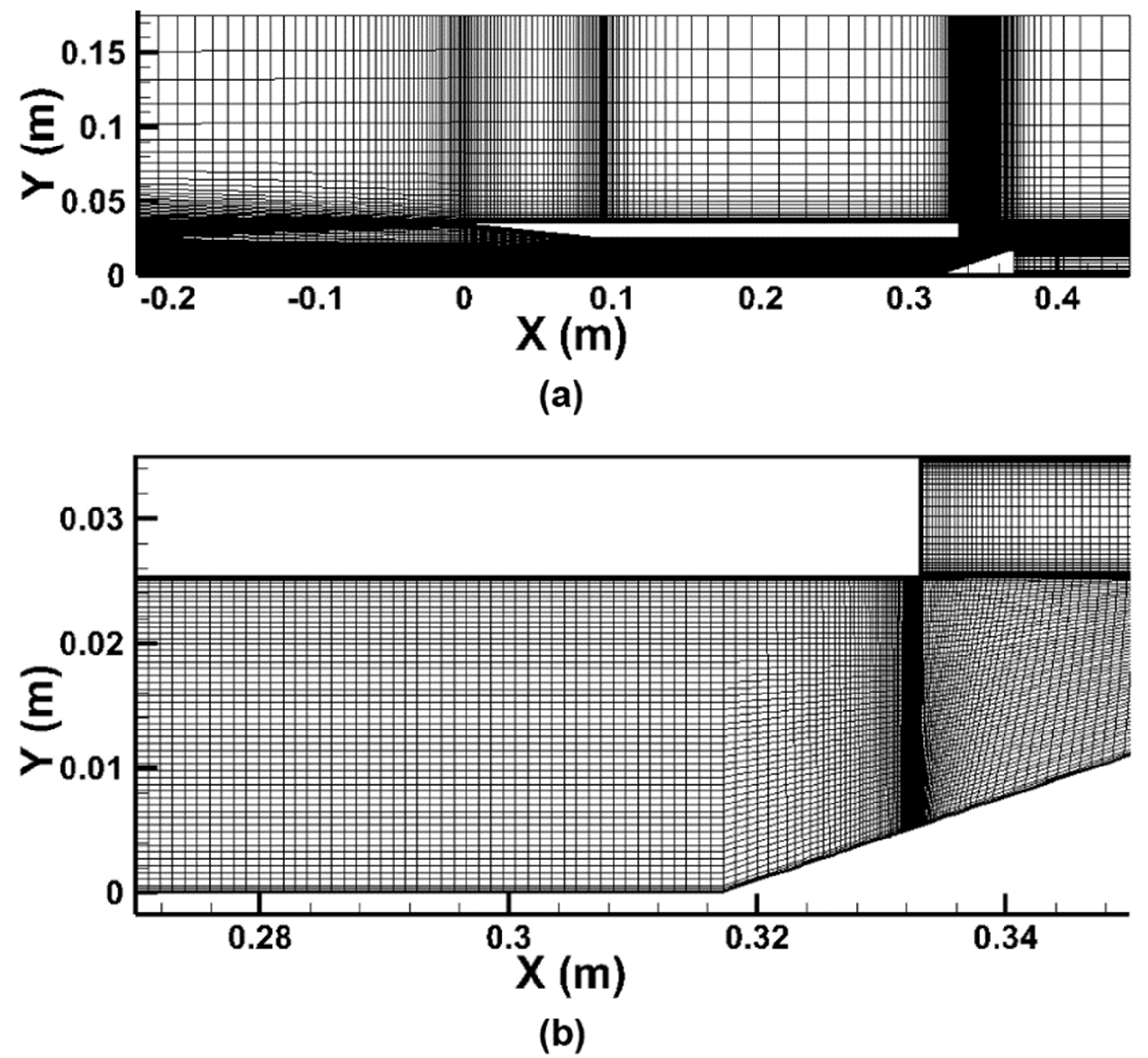Figure 2 shows the computational domain with Grid 4 for the scramjet inlet-isolator model. The inflow boundary conditions are the same as those described in Figure 1, and the outlet boundary conditions employ the supersonic outflow condition. The wall boundary conditions employ the no-slip adiabatic condition.

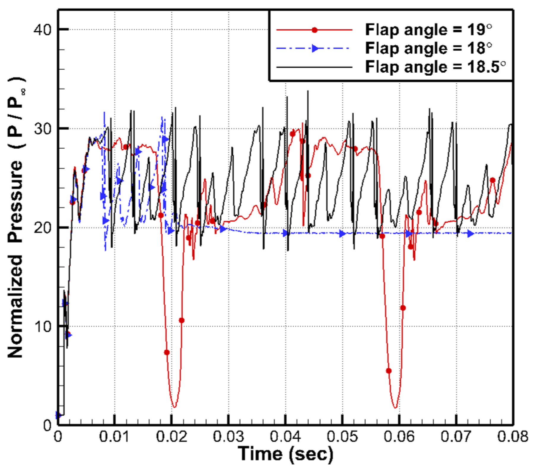
To simulate the back pressure, a flap is installed at the rear of the model. In the experimental paper, there was no information about the flap angle at the moment when ‘non-oscillatory unstarted flow’ appeared. Thus, to find the flap angle that shows ‘non-oscillatory unstarted flow’, case studies with changing flap angle are performed.

Figure 2 shows the grid system of the scramjet inlet-isolator model. As shown in the figure, dense grids are placed inside the inlet to simulate complex flow phenomena such as shock-boundary layer interactions. The total number of grid cells is approximately 42,000. For grid resolution analysis, we compare the numerical results doubling the number of grids, but there are no significant differences in the results. The inflow boundary conditions are the same as those described in Figure 1, and the outlet boundary condition employed the supersonic outflow condition. The wall boundary conditions employ the no-slip adiabatic condition.

3. Results and Discussion

3.1. Inlet Unstart Mode Transition with Different Flap Angles

In the experimental results of Wagner, ‘non-oscillatory unstarted flow’ showed nonperiodic characteristics, and the normalized pressure ($\mathrm{P}/{\mathrm{P}}_{\infty }$) oscillated between 20 and 30 [11]. However, the exact flap angle for ‘non-oscillatory unstarted flow’ was not provided in the paper. Therefore, in this study, case studies are performed by changing the flap angles to find the flap angle for ‘non-oscillatory unstarted flow’. For convenience, ‘high-amplitude oscillatory unstarted flow’ is denoted as HAO mode. ‘Non-oscillatory unstarted flow’ is denoted as NO mode.

Of the various numerical results, the results with flap angles of 19°, 18°, and 18.5° are presented in this section. Figure 3 shows the time history of the normalized pressure near the flap (x/h = 12.21) with various flap angles. As shown in the figure, for a flap angle of 19°, the normalized pressure ($\mathrm{P}/{\mathrm{P}}_{\infty }$) value oscillates between 1 and 30 with periodicity. Additionally, the pressure decreases to freestream pressure (${\mathrm{P}}_{\infty }$) levels near time = 0.02 and 0.06 s. As shown in a previous study, this pressure oscillation is a typical pressure pattern of HAO mode [15]. The high-pressure region near the flap generated by the reduced flow passage results in backflow within the model. Eventually, the strong backflow escapes out of the model and results in pressure release to the freestream pressure level.

For a flap angle of 18°, the normalized pressure ($\mathrm{P}/{\mathrm{P}}_{\infty }$) value oscillates between 20 and 30, which is the same pressure oscillation range in NO mode that appeared in the experiment [11]. However, after 0.04 s, the pressure no longer oscillates and represents a constant value. Figure 4 shows the Mach number contour for a flap angle of 18° at time = 0.05 s. As shown in the figure, supersonic flow exists in the entire flow passage without disconnection, so the inlet is started. Therefore, at a flap angle of 18°, the inlet state is at the boundary between NO mode and the inlet start state.

Since the flap angle of 19° shows HAO mode and the flap angle of 18° shows a transitional state between NO mode and the inlet start state, it is expected that a stable NO mode can be obtained between flap angles of 18° and 19°. Therefore, an additional numerical test is performed for the flap angle of 18.5° and presented in Figure 3.

As shown in the figure, for a flap angle of 18.5°, the normalized pressure ($\mathrm{P}/{\mathrm{P}}_{\infty }$) value oscillates between 20 and 30 overall. However, unlike HAO mode, the peak pressure value of this case changes with time, so the pressure oscillation is nonperiodic.

Table 2. Comparison of pressure oscillation characteristics at x/h = 12.21 with experimental data.

	Experiment [11]	Present (Flap Angle = 18.5°)
Periodicity	nonperiodic	nonperiodic
$\mathrm{Average}\mathrm{amplitude}\mathrm{of}\mathrm{oscillation}{\left(\Delta \mathrm{P}/{\mathrm{P}}_{\infty }\right)}_{ave}$	10	9.9 (error = 1%)
$\mathrm{Average}\mathrm{pressure}({\mathrm{P}}_{ave}/{\mathrm{P}}_{\infty }$)	23.9	24.16 (error = 1.1%)

shows the summary of the pressure oscillation characteristics for a flap angle of 18.5° and a comparison with the experimental results. As shown in the table, the nonperiodic oscillation pattern and the range of the pressure oscillation in this case are in good agreement with the experimental results [11]. Therefore, a flap angle of 18.5° is selected as a representative case of NO mode.

3.2. Pressure Oscillation Patterns in NO Mode

In this section, we investigate the flow characteristics and the mechanism of NO mode using the numerical test result for a flap angle of 18.5°.

Figure 5 shows the time history of the normalized pressure ($\mathrm{P}/{\mathrm{P}}_{\infty }$) near the flap (x/h = 12.21) for the flap angle of the 18.5° case. As shown in the figure, the normalized pressure value oscillates between 20 and 30 overall. However, in some oscillations, the normalized peak pressure is less than 25. To understand the entire flow characteristics of NO mode, these two pressure oscillation patterns are analyzed separately. Pattern 1 (the solid box in the figure) is the pressure oscillation between 20 and 30. Pattern 2 (the dotted box in the figure) is the pressure oscillation with relatively low peak pressure.

Furthermore, to investigate the flow characteristics in detail, several time points are selected (points [a]~[d] and points [${\mathrm{a}}_2$]~[${\mathrm{d}}_2$] in the figure). Points [a] and [${\mathrm{a}}_2$] represent the moments with minimum pressure. Points [b] and [${\mathrm{b}}_2$] represent moments with similar pressure levels when the pressure is rising. Points [c] and [${\mathrm{c}}_2$] represent the moments with peak pressure during the oscillation. Points [d] and [${\mathrm{d}}_2$] represent moments with similar pressure levels when the pressure is decreasing. Additionally, point [c′] is selected as the moment with the same pressure level as point [${\mathrm{c}}_2$].

To investigate the characteristics of Pattern 1, the axial velocity and normalized pressure ($\mathrm{P}/{\mathrm{P}}_{\infty }$) contours and velocity vectors at the moments of [a], [b], [c], and [d] are shown in Figure 6. Figure 6a shows the moment of point [a], which represents the minimum downstream pressure. As shown in Figure 6(a-1), there is a backflow (negative axial velocity) region along the lower wall of the model. Due to the backflow, the normalized pressure ($\mathrm{P}/{\mathrm{P}}_{\infty }$) value decreases to approximately 20 near the downstream of the model in Figure 6(a-2).

Figure 6b shows the moment of point [b] when the downstream pressure starts to increase. As shown in Figure 6(b-1), the low back pressure generated at point [a] results in the re-entry of the flow along the lower wall downstream. Therefore, in Figure 6(b-2), re-entering the flow results in a pressure increase near the exit.

Figure 6c shows the moment of point [c] when the downstream pressure reaches a maximum. From point [b] to [c], continuous re-entering of the flow results in the maximum downstream pressure in Figure 6(c-2). In this case, the normalized pressure at x/h = 12.21 is approximately 30.8. Furthermore, in Figure 6(c-1), due to the adverse pressure profiles, backflow and recirculation zones are generated along the upper and lower walls of the model.

Figure 6d shows the moment of point [d] when the downstream pressure has decreased. From point [c], the adverse pressure profile results in backflow. The continuous backflow shown in Figure 6(d-1) results in a downstream pressure decrease, as shown in Figure 6(d-2). After point [d], the axial velocity distributions and normalized pressure distributions become similar to those in Figure 6a, and these flow patterns are found to be repeated.

In the same manner, to investigate the flow mechanism of Pattern 2, the axial velocity and normalized pressure ($\mathrm{P}/{\mathrm{P}}_{\infty }$) contours and velocity vectors at the moments of [${\mathrm{a}}_2]$, [${\mathrm{b}}_2]$, [${\mathrm{c}}_2],$ and [${\mathrm{d}}_2]$ are shown in Figure 7. Figure 7a shows the moment of point [${\mathrm{a}}_2$], which represents the minimum downstream pressure. Similar to Figure 6a, there is a small backflow region along the lower wall of the model, and the normalized pressure ($\mathrm{P}/{\mathrm{P}}_{\infty }$) value decreases to approximately 20 near the downstream of the model.

Figure 7b shows the moment of point [${\mathrm{b}}_2$] when the downstream pressure of the inlet increases. Similar to Figure 6b, the low back pressure generated at point [${\mathrm{a}}_2]$ results in the re-entry of the flow along the lower wall downstream in Figure 7(b-1). In Figure 7(b-2), re-entering the flow results in a pressure increase near the exit.

Figure 7c shows the moment of point [${\mathrm{c}}_2]$ when the downstream pressure reaches its local maximum. As shown in Figure 7(c-2), continuous re-entry of the flow results in an increase in downstream pressure. However, in Figure 7(c-2), the normalized pressure at x/h=12.21 is only approximately 23.9, which is less than that at point [c]. Furthermore, the recirculation zone of the upper wall shown in Figure 6(c-1) is not shown in Figure 7(c-1).

Figure 7d shows the moment of point [${\mathrm{d}}_2]$ when the downstream pressure has decreased. As shown in the figure, the adverse pressure profile results in backflow along the lower wall. The continuous backflow shown in Figure 7(d-1) results in a downstream pressure decrease, as shown in Figure 7(d-2). After point [${\mathrm{d}}_2]$, the axial velocity distributions and normalized pressure distributions become similar to those in Figure 7a, and these flow patterns are found to be repeated.

3.3. Detailed Analysis of Nonperiodic Phenomena in NO mode

In the previous section, to understand the buzz mechanisms in Patterns 1 and 2, the axial velocity and normalized pressure ($\mathrm{P}/{\mathrm{P}}_{\infty }$) contours and velocity vectors are reviewed through Figure 6 and Figure 7. In these figures, the basic physical phenomena of these two patterns are similar. However, the two patterns have different local maximum back pressures and different flow configurations such as recirculation zones and backflow areas. Despite the observations in Figure 6 and Figure 7, the reason for the differences in Patterns 1 and 2 is still unclear.

In this section, to determine the causes of these differences, the flow characteristics of Patterns 1 and 2 are compared and analyzed in more detail.

Figure 8 shows the Mach number and the normalized pressure contours and velocity vectors at the moments of points [b] and [${\mathrm{b}}_2$] marked in Figure 5. In Figure 8a,b, Patterns 1 and 2 have two subsonic zones, LB1 (Lower Bubble 1) and LB2 (Lower Bubble 2), at the lower wall. Originally, before these moments, a long boundary layer is located on the lower wall, as shown in Figure 6a and Figure 7a. However, due to the blockage effects of the thick boundary layer on the front, the supersonic inflow is deflected upward and bounces back from the upper front wall to hit the middle of the lower wall, as marked by the red arrows in the figure. Due to the supersonic flow impact on the lower wall, the long boundary layer is divided into two subsonic zones, LB1 and LB2.

After the impact on the lower wall, the supersonic flow bounces back to the upper wall again. As marked by solid red circles in Figure 8c,d, the bounced flow generates a local high-pressure zone on the upper wall. This local high-pressure zone prevents inflow and generates another separation zone UB (upper bubble) on the upper wall, as shown in Figure 8a,b. As shown in Figure 8, Patterns 1 and 2 show similar flow configurations thus far.

Figure 9 shows the Mach number and the normalized pressure contours and velocity vectors at the moments of point [c′] and point [${\mathrm{c}}_2$] marked in Figure 5. At this time, point [c′] is selected as the moment with the same pressure level as point [${\mathrm{c}}_2$]. Despite having the same pressure levels, Patterns 1 and 2 show very different flow configurations in Figure 9. In Figure 9a for Pattern 1, the two subsonic zones, LB1 and LB2, remain separated. The separation zone UB on the upper wall also exists. However, in Figure 9b, for Pattern 2, LB1 and LB2 merge into one boundary layer, and UB on the upper wall disappears. Furthermore, in the enlarged drawing of Figure 9a, subsonic flow occupies the entire flow passage in some areas downstream, resulting in choked flow. However, in the enlarged drawing of Figure 9b, the supersonic zone reaches the outlet without disconnection, so the flow is not choked. When UB on the upper wall disappears in Figure 9b, the flow passage expands, so the high pressure is released at this moment. Therefore, in Figure 5, the pressure of Pattern 1 continues to increase after [c′], but Pattern 2 decreases after [${\mathrm{c}}_2$].

It is not so clear why UB disappeared in Figure 9b. However, as shown in Figure 8a, UB is generated by the third collision of the supersonic inflow into the wall. Therefore, slight differences in the inflow conditions from upstream may affect the state of the wall collisions and change the presence of UB on the upper wall. In other words, the presence of UB on the upper wall is so unstable that it can be generated or extinguished irregularly. For this reason, as shown in Figure 5, Patterns 1 and 2 irregularly appear in NO mode, resulting in nonperiodic characteristics.

3.4. Differences between HAO Mode and NO Mode

In a previous study, the characteristics of HAO mode were analyzed [15]. In the previous section, the characteristics of NO mode are explained. In this section, we compare HAO mode with NO mode and analyze the differences between them and the causes for these two inlet unstart modes.

Figure 10 shows the time histories of the normalized pressure ($\mathrm{P}/{\mathrm{P}}_{\infty }$) near the flap (x/h = 12.21) for HAO mode and NO mode. As shown in the figure, the pressure oscillation pattern shows periodicity for HAO mode but non-periodicity for NO mode. Furthermore, in HAO mode, the minimum normalized pressure ($\mathrm{P}/{\mathrm{P}}_{\infty }$) reaches a nearly free stream pressure level. The maximum normalized pressure reaches approximately 34, which is higher than the maximum value of 30 in NO mode. On the other hand, the normalized pressure in NO mode oscillates between 20 and 30 overall.

To investigate the reasons for these differences, four time points [a], [b], [c], and [d], are selected from HAO mode in Figure 10.

Point [a] represents the moment of the minimum pressure, and point [b] represents a moment during the pressure rise. Point [c] represents the moment of the maximum pressure, and point [d] represents the moment during the pressure decrease.

Figure 11 shows the axial velocity and normalized pressure ($\mathrm{P}/{\mathrm{P}}_{\infty }$) contours and velocity vectors at the moments of [a], [b], [c], and [d]. In Figure 11a, the pressure decreases to the free stream pressure level. Due to the low back pressure, the inflow enters the model without any resistance. However, in Figure 11b, due to the excessive inflow, the back pressure downstream starts to rise. In some part of the axial velocity contour, there exists a separation zone and negative axial velocity area. In Figure 11c, the back pressure reaches its maximum, and the backflow (negative axial velocity) becomes more remarkable upstream. Finally, in Figure 11d, the backflow occupies most of the flow passage within the model. Furthermore, the backflow escapes very actively out of the model, and there is no incoming flow from the upstream of the model. Due to the active backflow, the high back pressure decreases to approximately 13, as shown in Figure 10. After this point, the sufficient back pressure release results in incoming flow recovery and returns to the state at point [a].

To see the difference between HAO mode and NO mode, we can compare Figure 7 and Figure 11. In both figures, the incoming flow results in a back pressure increase. The higher back pressure results in backflow. Finally, the backflow results in back pressure release. These mechanisms are similar. However, important differences can be found in Figure 7d and Figure 11d. In HAO mode, as shown in Figure 11d, the active back flow occupies the most flow passage within the model. There is no incoming flow from the upstream of the model. On the other hand, in NO mode, as shown in Figure 7d, the incoming flow and the backflow coexist in the flow passage. Therefore, the back pressure release is rather insufficient in NO mode. This is why the minimum pressure is approximately 20 in NO mode but almost 1 in HAO mode. The differences between Figure 7d and Figure 11d are due to the maximum back pressure level in Figure 7c and Figure 11c. The maximum back pressure is approximately 34 in HAO mode, as shown in Figure 11c, but approximately 23.9 in NO mode, as shown in Figure 7c. As a result, a high back pressure causes active backflow in HAO mode.

The maximum back pressure differences between HAO mode and NO mode can be due to the different exit areas of the model. In HAO mode, 41.5% of the exit area is blocked by the flap. However, in NO mode, only 20.7% of the exit area is blocked by the flap. If the flow is choked at the exit, the total pressure of the flow is inversely proportional to the exit area, as shown in Equation (1).

$$P_t=\frac{\dot{m}}{A^{*}}\frac{\sqrt{R{T}_t}}{\sqrt{\gamma }{\left(\frac{\gamma +1}{2}\right)}^{\left(\gamma +1\right)/\left(2-2\gamma \right)}}$$

(1)

Therefore, with the same amount of inflow, HAO mode shows a higher maximum back pressure than NO mode.

4. Conclusions

In this study, the characteristics and mechanisms of ‘non-oscillatory unstarted flow’ (NO mode) that appeared in Wagner’s experiment were investigated using numerical analysis. ‘High-amplitude oscillatory unstarted flow’ (HAO mode), which was another inlet unstart mode in the experiment, was compared with NO mode. Before the detailed analysis, a case study was performed to find the appropriate flap angle for NO mode appearing in the experiment. Because of the fair agreement with the experimental results, a flap angle of 18.5° was chosen for the representative case of NO mode.

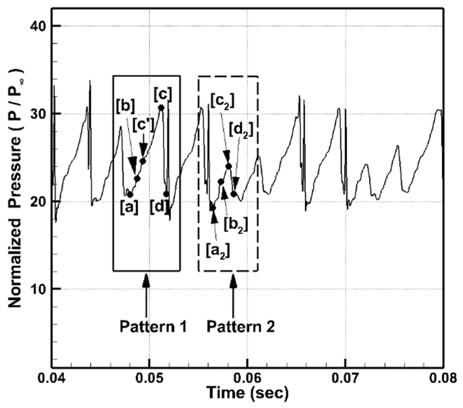
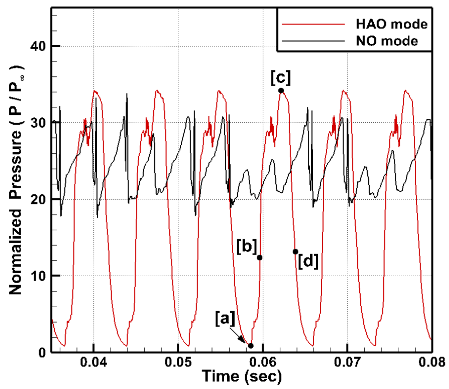
From the observation of the pressure oscillation patterns, there were two different oscillation patterns in NO mode. In Pattern 1, the normalized pressure ($\mathrm{P}/{\mathrm{P}}_{\infty }$) value oscillated between 20 and 30. However, in Pattern 2, the normalized peak pressure was less than 25. These two patterns appeared irregularly, so the oscillation was nonperiodic in NO mode.

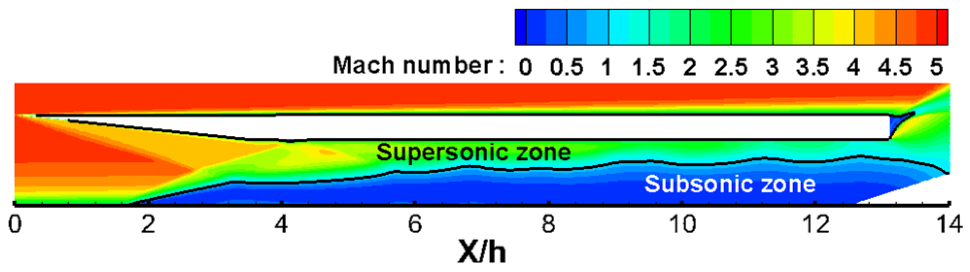
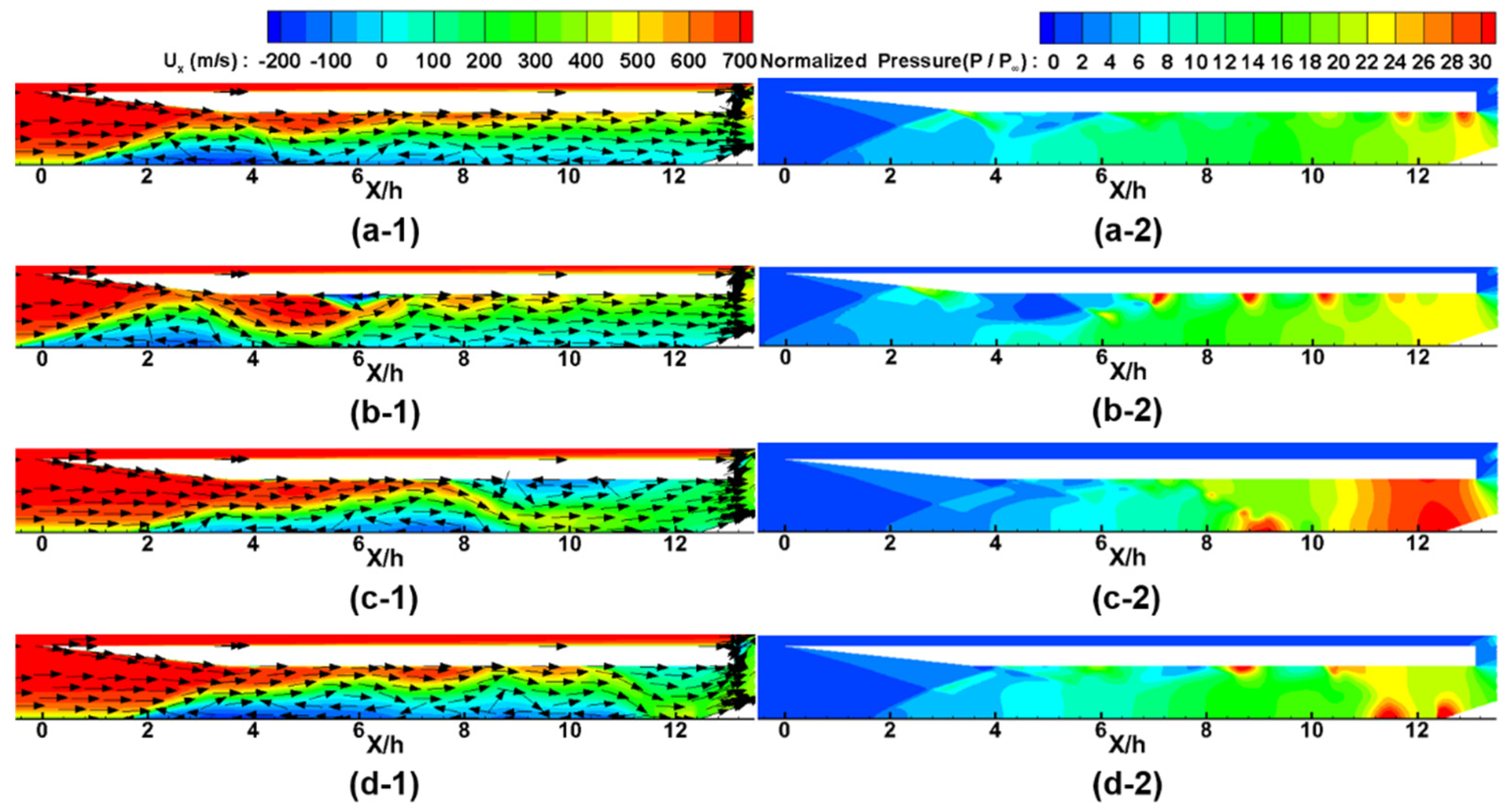
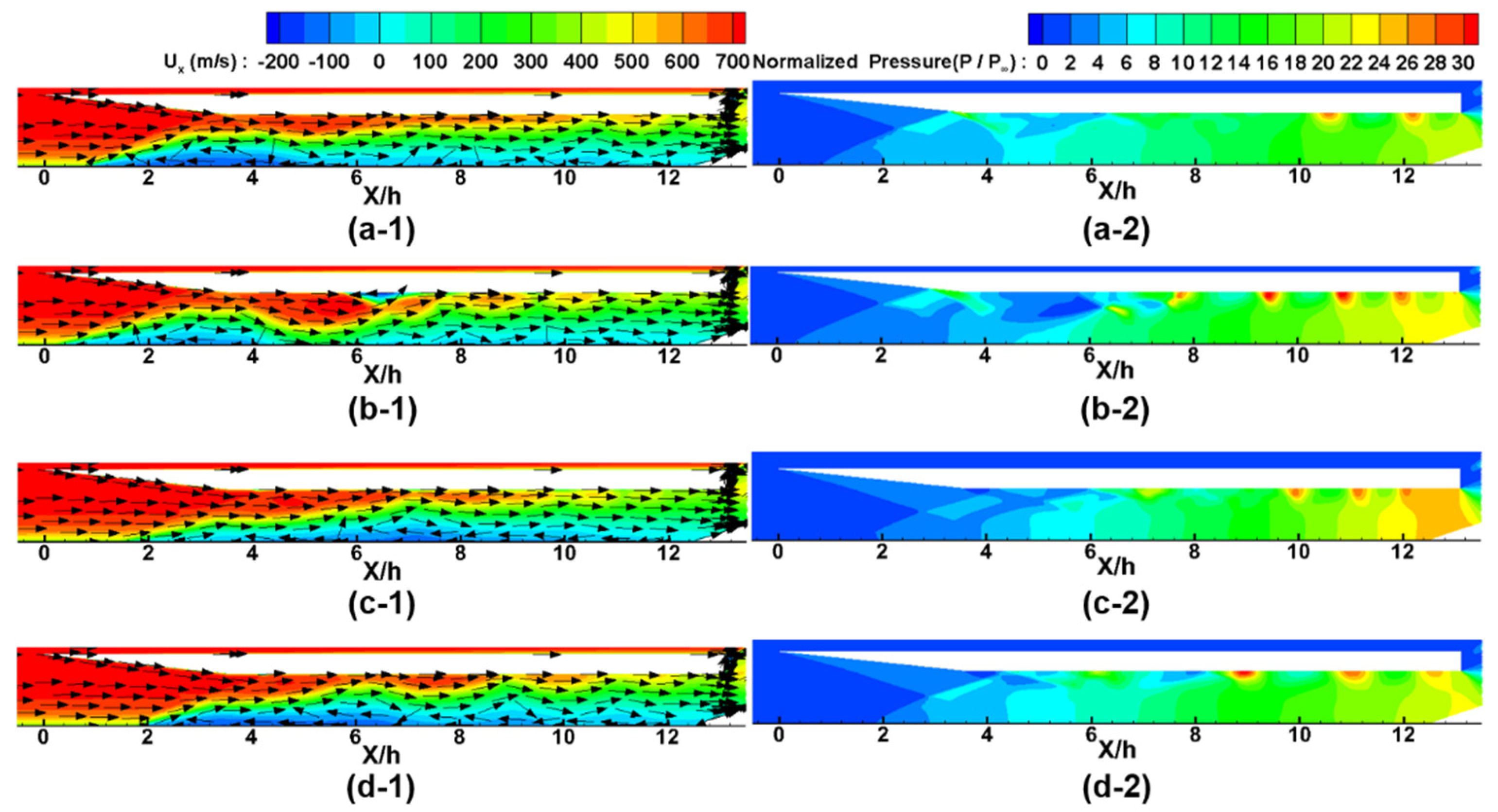
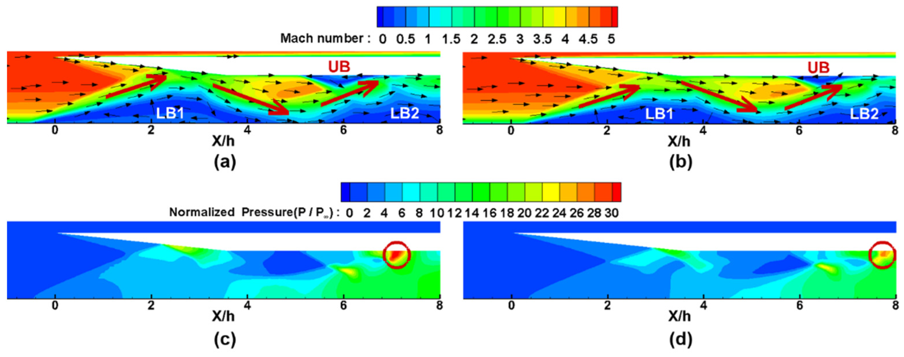
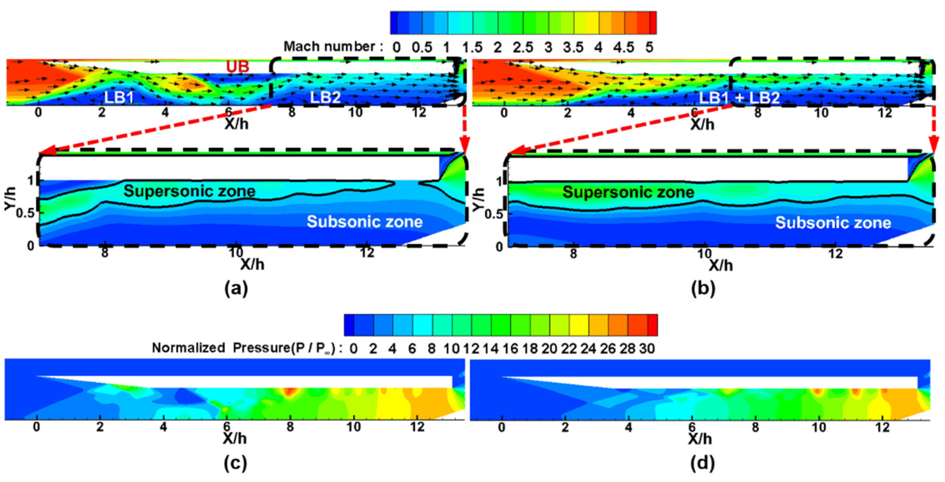
To understand the flow characteristics and mechanisms of NO mode, two pressure oscillation patterns were analyzed and compared. In the results, the basic pressure oscillation mechanisms were similar in both patterns. The back pressure increase with the inflow, the backflow due to the higher back pressure, and the back pressure decrease due to the backflow were the same in both patterns. However, the two patterns had different local maximum back pressures and different flow configurations. In the results of a more detailed analysis, a separation zone on the upper wall (UB) was generated by the third collision of the supersonic inflow into the wall in both patterns. However, slight differences in the inflow conditions from upstream may affect the state of the wall collisions, so UB could be generated or disappear irregularly. When UB was generated, it blocked the flow passage and resulted in a pressure rise. However, when UB disappeared, the back pressure was released due to flow passage expansion.

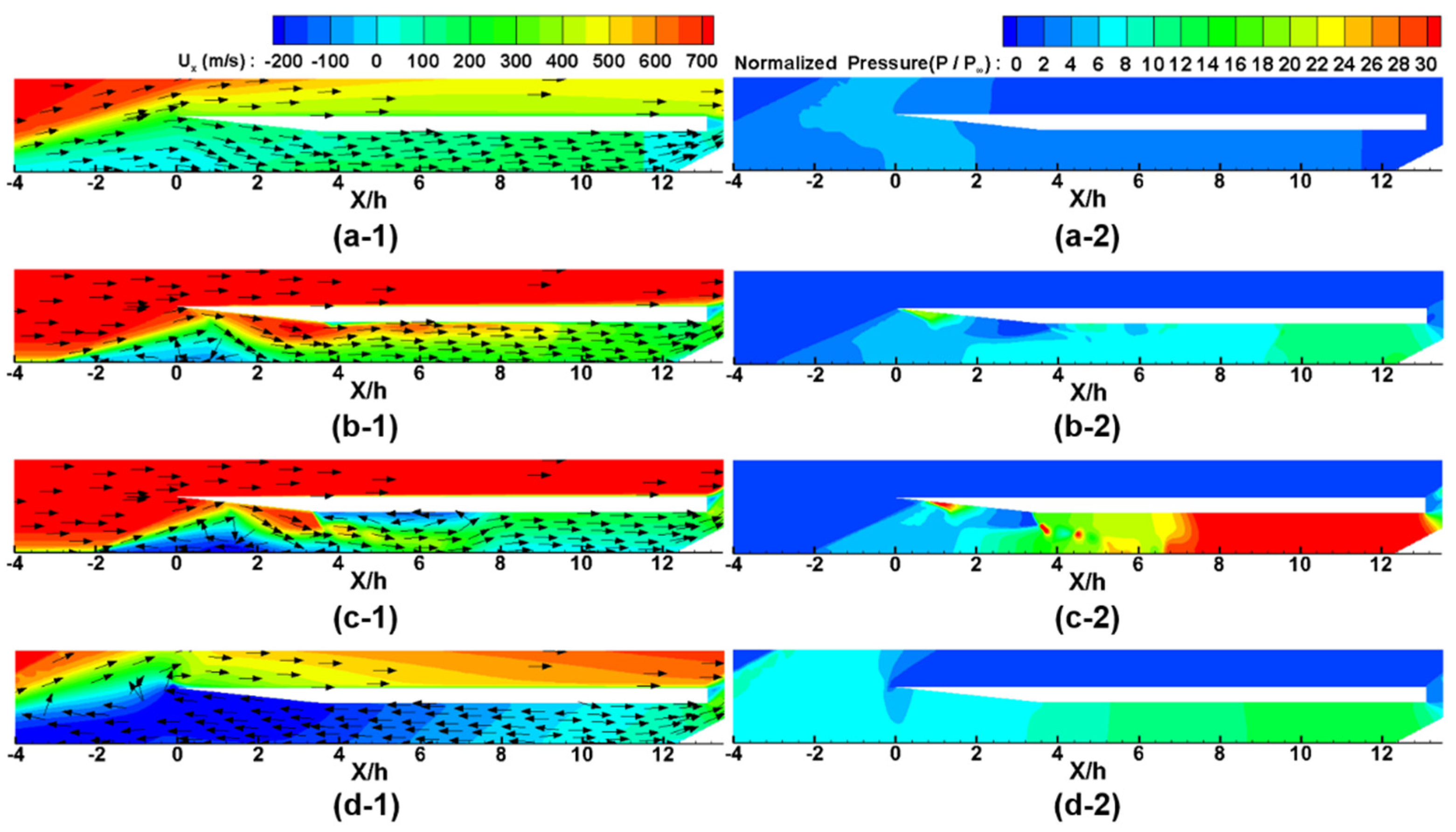
Additionally, the flow characteristics of HAO mode and NO mode were compared. In HAO mode, due to the high back pressure downstream, the backflow was very active and occupied the most flow passage. On the other hand, NO mode showed a relatively low peak pressure compared to that of HAO mode, and the incoming flow and the backflow coexisted in the flow passage. Therefore, the back pressure release was rather insufficient. The maximum back pressure differences between HAO mode and NO mode were due to the different exit areas of the model. The exit area of HAO mode was approximately half of the exit area of NO mode.

References

1. Oswatitsch, K. Pressure Recovery for Missiles with Reaction Propulsion at High Supersonic Speeds (The Efficiency of Shock Diffusers). In Contributions to the Development of Gasdynamics; Vieweg+Teubner Verlag: Berlin, Germany, 1980; pp. 290–323. [Google Scholar]
2. Ferri, A.; Nucci, L.M. The Origin of Aerodynamic Instability of Supersonic Inlets at Subcritical Conditions; NACA Report, Report No. NACA-RM-L50K30; NACA: Washington, DC, USA, 1951. [Google Scholar]
3. Dailey, C.L. Supersonic Diffuser Instability. Ph.D. Thesis, California Institute of Technology, Pasadena, CA, USA, 1954. [Google Scholar]
4. Fisher, S.A.; Neale, M.C.; Brooks, A.J. On the Sub-Critical Stability of Variable Ramp Intakes at Mach Numbers around 2; Aeronautical Research Council Report, Report No. ARC-R/M-3711; Cranfield University: Cranefield, UK, 1970; pp. 1–35. [Google Scholar]
5. Trapier, S.; Duveau, P.; Deck, S. Experimental Study of Supersonic Inlet Buzz. AIAA J. 2006, 44, 2354–2365. [Google Scholar] [CrossRef]
6. Trapier, S.; Deck, S.; Duveau, P. Delayed Detached-Eddy Simulation and Analysis of Supersonic Inlet Buzz. AIAA J. 2008, 46, 118–131. [Google Scholar] [CrossRef]
7. Murthy, S.N.B.; Curran, E.T. Scramjet Propulsion, Progress in Astronautics and Aeronautics; AIAA Inc.: Reston, VA, USA, 2001; pp. 447–511. [Google Scholar]
8. Chang, J.; Li, N.; Xu, K.; Bao, W.; Yu, D. Recent research progress on unstart mechanism, detection and control of hypersonic inlet. Prog. Aerosp. Sci. 2017, 89, 1–22. [Google Scholar] [CrossRef]
9. Tan, H.-J.; Guo, R.-W. Experimental Study of the Unstable-Unstarted Condition of a Hypersonic Inlet at Mach 6. J. Propuls. Power 2007, 23, 783–788. [Google Scholar] [CrossRef]
10. Tan, H.-J.; Sun, S.; Yin, Z.-L. Oscillatory Flows of Rectangular Hypersonic Inlet Unstart Caused by Downstream Mass-Flow Choking. J. Propuls. Power 2009, 25, 138–147. [Google Scholar] [CrossRef]
11. Wagner, J.L. Experimental Studies of Unstart Dynamics in Inlet/Isolator Configurations in a Mach 5 Flow. Ph.D. Thesis, University of Texas, Austin, TX, USA, 2009. [Google Scholar]
12. Tan, H.-J.; Li, L.-G.; Wen, Y.-F.; Zhang, Q.-F. Experimental Investigation of the Unstart Process of a Generic Hypersonic Inlet. AIAA J. 2011, 49, 279–288. [Google Scholar] [CrossRef]
13. Li, Z.; Gao, W.; Jiang, H.; Yang, J. Unsteady Behaviors of a Hypersonic Inlet Caused by Throttling in Shock Tunnel. AIAA J. 2013, 51, 2485–2492. [Google Scholar] [CrossRef]
14. Koo, H.; Raman, V. Large-Eddy Simulation of a Supersonic Inlet-Isolator. AIAA J. 2012, 50, 1596–1613. [Google Scholar] [CrossRef]
15. Lee, J.; Kang, S.H. Numerical study on the start and unstart phenomena in a scramjet inlet-isolator model. PLoS ONE 2019, 14, e0224994. [Google Scholar] [CrossRef] [PubMed] [Green Version]
16. Espinoza, D.E.; Scanlon, T.J.; Brown, R.E. Validation of Tools to Accelerate High-Speed CFD Simulations Using OpenFOAM. In Proceedings of the 20th AIAA International Space Planes and Hypersonic Systems and Technologies Conference, Glasgow, Scotland, 6–9 July 2015; pp. 1–18. [Google Scholar]
17. Greenshields, C.J.; Weller, H.G.; Gasparini, L.; Reese, J.M. Implementation of semi-discrete, non-staggered central schemes in a colocated, polyhedral, finite volume framework, for high-speed viscous flows. Int. J. Numer. Methods Fluids 2009, 63, 1–21. [Google Scholar] [CrossRef] [Green Version]
18. Kurganov, A.; Noelle, S.; Petrova, G. Semi-discrete central-upwind schemes for hyperbolic conservation laws and Hamilton-Jacobi equations. SIAM J. Sci. Comput. 2001, 160, 241–282. [Google Scholar]
19. Sutherland, W. The viscosity of gases and molecular force. Philos. Mag. Ser. 5 1893, 36, 507–531. [Google Scholar] [CrossRef] [Green Version]
20. Menter, F.R.; Kuntz, M.; Langtry, R. Ten Years of Industrial Experience with the SST Turbulence Model. In Proceedings of the 4th Internal Symposium of Turbulence, Heat and Mass Transfer, Antalya, Turkey, 12–17 October 2003; pp. 625–632. [Google Scholar]
21. Dorofeeva, O.; Novikov, V.P.; Neumann, D.B. NIST-JANAF thermochemical tables. I. ten organic molecules related to atmospheric chemistry. J. Phys. Chem. Ref. Data 2001, 30, 475–513. [Google Scholar] [CrossRef] [Green Version]
22. Wilcox, D.C. Turbulent Modeling for CFD, 2nd ed.; DCW Industries Inc.: La Canada, CA, USA, 1998. [Google Scholar]
23. Shin, H.; Park, S.H.; Byun, Y.H. A Two-Dimensional Numerical Analysis of the Unstart Process in an Inlet/Isolator Model. In Proceedings of the 2017 KSPE Spring Conference, Jeju, Korea, 31 May–2 June 2017; pp. 341–345. [Google Scholar]
Figure 1. Schematic of the scramjet inlet-isolator model.
Aerospace 09 00162 g001
Figure 2. Computational grid for the inlet-isolator model: (a) grid for the entire domain; (b) enlarged picture of the grid near the model outlet.
Aerospace 09 00162 g002
Figure 3. Comparison of the pressure time history at x/h = 12.21 with various flap angles.
Aerospace 09 00162 g003
Figure 4. Mach number contours for the flap angle of 18° at time = 0.05 s.
Aerospace 09 00162 g004
Figure 5. Time history of normalized pressure at x/h = 12.21 with a flap angle of 18.5°.
Aerospace 09 00162 g005
Figure 6. Axial velocity contours with velocity vectors (left) and normalized pressure contours (right) for Pattern 1: (a-1) axial velocity at point [a]; (a-2) normalized pressure at point [a]; (b-1) axial velocity at point [b]; (b-2) normalized pressure at point [b]; (c-1) axial velocity at point [c]; (c-2) normalized pressure at point [c]; (d-1) axial velocity at point [d]; (d-2) normalized pressure at point [d].
Aerospace 09 00162 g006
Figure 7. Axial velocity contours with velocity vectors (left) and normalized pressure contours (right) for Pattern 2: (a-1) axial velocity at point [ a 2 ]; (a-2) normalized pressure at point [ a 2 ]; (b-1) axial velocity at point [ b 2 ]; (b-2) normalized pressure at point [ b 2 ]; (c-1) axial velocity at point [ c 2 ]; (c-2) normalized pressure at point [ c 2 ]; (d-1) axial velocity at point [ d 2 ]; (d-2) normalized pressure at point [ d 2 ].
Aerospace 09 00162 g007
Figure 8. Comparison of the flow configurations of Patterns 1 and 2: (a) Mach number, velocity vectors at point [b] (Pattern 1); (b) Mach number, velocity vectors at point [ b 2 ] (Pattern 2); (c) normalized pressure at point [b] (Pattern 1); (d) normalized pressure at point [ b 2 ] (Pattern 2).
Aerospace 09 00162 g008
Figure 9. Comparison of the flow configurations of Patterns 1 and 2: (a) Mach number, velocity vectors at point [c’] (Pattern 1); (b) Mach number, velocity vectors at point [ c 2 ] (Pattern 2); (c) normalized pressure at point [c’] (Pattern 1); (d) normalized pressure at point [ c 2 ] (Pattern 2).
Aerospace 09 00162 g009
Figure 10. Time histories of the normalized pressure at x/h = 12.21 in HAO mode and NO mode.
Aerospace 09 00162 g010
Figure 11. Axial velocity contours with the velocity vectors (left) and normalized pressure contours (right) for HAO mode: (a-1) axial velocity at point [a]; (a-2) normalized pressure at point [a]; (b-1) axial velocity at point [b]; (b-2) normalized pressure at point [b]; (c-1) axial velocity at point [c]; (c-2) normalized pressure at point [c]; (d-1) axial velocity at point [d]; (d-2) normalized pressure at point [d].
Aerospace 09 00162 g011