Article

A Multidisciplinary Possibilistic Approach to Size the Empennage of Multi-Engine Propeller-Driven Light Aircraft

Department of Aerospace Engineering, Ryerson University, Toronto, ON M5B 2K3, Canada
*
Author to whom correspondence should be addressed.
Aerospace 2022, 9(3), 160; https://doi.org/10.3390/aerospace9030160
Submission received: 3 January 2022 / Revised: 4 March 2022 / Accepted: 11 March 2022 / Published: 15 March 2022
(This article belongs to the Section Aeronautics)

Abstract

:
In considering aircraft design, it is very important to effectively size the tail configuration for stability and control. Multidisciplinary design optimization (MDO) focuses on the use of numerical optimization in the design of systems with multiple subsystems or disciplines of consideration. However, MDO uses deterministic calculations, and does not consider the uncertainties that arise from the employed analyses, including errors due to linearization and simplification. For problems with inadequate input data, the possibility-based design optimization (PBDO) scheme can be implemented in its stead to achieve reliable designs using membership functions for epistemic uncertainties. A multidisciplinary, possibilistic approach is presented to define the sizing of the empennage configuration of a twin-engine propeller-driven aircraft by changing shape parameters while satisfying the design requirements given the tailless aircraft configuration, the flight conditions, and various uncertainties. The corresponding disciplines are aerodynamics, stability and control, propulsion and weight and balance. Herein, different design requirements are considered including longitudinal/lateral/directional trim and stability characteristics, manufacturing and controllability criteria, handling qualities, operational requirements, airworthiness and survivability. The resulting aerodynamic characteristics and flight dynamic stability outcomes show that the optimized tail configuration for the proposed aircraft fully complied with airworthiness requirements and predefined constraints while considering several uncertainties due to the use of early-stage statistical estimations. The proposed approach can be used to enhance the preliminary design of multi-engine propeller-driven light aircraft where only low-fidelity, statistical estimations are available. The resulting output is not only an optimized aircraft configuration, but one where the stability of the design has been ensured. In this work, the aerodynamic characteristics have been determined using a validated semi-empirical program called MAPLA, developed for light aircraft designs and development in the preliminary design phase. Furthermore, the optimization framework consists of a deterministic optimizer that runs sequentially with a possibility assessment algorithm.

1. Introduction

Traditional civil aircraft design and development is mainly focused on providing vehicles that meet performance requirements while minimizing operational costs. This meant that a sequential strategy was required to address changing assumptions as the design matured, with no promise for an ideal design as the designer was faced with a complex multidisciplinary procedure [1]. Earlier designers were forced to rely on their creative and qualitative knowledge due to the lack of computational analysis and computer aided tools in the beginning of the conceptual design stage. As such, it was very difficult to predict the exact penalties of altering certain variables, with core decisions being made through the use of existing information and repetitive, time-consuming studies in a loop until an acceptable configuration was found. As time passed, the market demanded products that could be as low-price as possible to be affordable by individuals while providing a safe, reliable, and efficient flight. Consequently, current aircraft design is extremely multifaceted, accounting for the interaction of multiple disciplines such as aerodynamics, performance, stability and control, propulsion, structures, avionics, and even environmental impacts [2]. To realize this time-consuming process, a massive investment in different analyses is required to modernize the design process [3]. Even though many different tools, such as the Finite Element Method (FEM) and Computational Fluid Dynamics (CFD), have been introduced to accelerate the aircraft design process and enhance the accuracy of estimations, principally in the preliminary and detailed design stages, the basic idea remains unchanged: to provide a cost-effective, high-quality vehicle that meets the required criteria of the desired mission. Hence, the aircraft design process still relies heavily on engineering information, historical statistics and low fidelity studies [4,5,6,7,8,9].
Modern aircraft design and development is a complex and involved process, requiring a decision-making process that combines multidisciplinary sequential calculations with the goal of balancing cost requirements and mission capabilities, all while various system criteria are considered. Thanks to computing developments, specifically in the areas of simulation tools and design procedures, more knowledge is now available in the earlier life-cycle stages, including the conceptual and preliminary design. As such, fewer penalties are associated with varying design variables in the modern process, providing a more efficient baseline product prior to the manufacturing phase. This was largely enabled by the now-abundant options for high-fidelity simulation tools [10,11,12,13].
The aircraft design and development process has extensively used different optimization techniques at different stages, but regardless of the iterative pathway, the result will only be as accurate as the original analysis methods they were built upon. Overall, both analytical and numerical optimization techniques, in spite of being incredibly powerful problem-solving tools, face several limitations when used for real engineering problems. Simply put, due to the linearization of calculations, simplification of analysis, and implementation of statistical and semi-empirical methods, some errors appear that spread over the optimization procedure. As such, optimizations in the early design stages face several restrictions due to the lack of accurate modelling and high-fidelity analysis, and the possibility emerges that the optimized design using low-fidelity estimations may fail to meet the required mission performance characteristics [14,15]. Consequently, it is imperative to understand the kind of error an aircraft development may face in the early stages of the design and development process, especially for guaranteeing the mission requirements while balancing the compromises made for effectiveness and affordability. Furthermore, knowledge about a specific type of aircraft typically enhances this optimization process and aids in developing viable designs, using experience gained through previous projects and available information about the specifications of existing designs in the same category [16,17,18,19].
Multidisciplinary design optimization (MDO) focuses on the use of numerical optimization in the design of systems with multiple subsystems or disciplines of consideration. The main reason for using MDO is that the performance of a system is related not only to each individual discipline, but also to their interactions. With the help of the MDO approach in the early design stages, one can simultaneously enhance the design while decreasing both the time and cost of the entire design cycle [20,21]. MDO has been a promising procedure for more than three decades, but it is still not as widely implemented in all the design phases as was initially expected [22,23,24,25,26,27,28,29,30,31]. Thus far, several methods have been proposed for MDO including: Multiple-discipline-feasible (MDF), Individual discipline feasible (IDF), All-at-once (AAO), and Simultaneous Analysis and Design (SAND) [20,21,22,23,24,25,26,27,28,29,30,31,32]. Some MDO structures have also been proposed based on the IDF and MDF methods. The IDF-based methods include Collaborative Optimization (CO), Enhanced Collaborative Optimization (ECO), Quasiseparable Decomposition (QSD), Exact and Inexact Penalty Decomposition (IPD/EPD) and Analytical Target Cascading (ATC). The MDF-based methods include Concurrent subspace optimization (CSSO), Bi-level integrated system synthesis (BLISS), Multidisciplinary design optimization based on independent subspaces (MDOIS) and Asymmetric Subspace Optimization (ASO) [20] MDO can improve the pace of conceptual design for an aircraft, quickly recognizing the optimal case through the use of simplified analyses that are available at this stage [33,34,35,36]. At its core, however, MDO relies upon deterministic calculations, and does not consider the uncertainties which arise from the defining assumptions of the employed analyses, including errors due to linearization and simplification.
The defining assumptions used for physical modelling open the process up to a risk of failure when a project transitions from paper to reality; a risk that can only be minimized with higher fidelity estimation, but never completely removed. Several works have been done to study the behavior of aleatory and epistemic uncertainty. Among those methods, some have been used for design optimization problems including Interval Analysis, Fuzzy Numbers, and Probability Theory. Generally, interval analysis or fuzzy numbers are preferred for cases where inadequate information is available to precisely determine the probability density function (PDF) [37,38,39,40].
Interval modeling is commonly used as a non-probabilistic representation of uncertainty [41,42]. The general concept is that some value Y cannot be determined with perfect accuracy but is known to lie between the boundaries A and B . Accordingly, any mathematical operation which is applied to Y can alternately be used on the interval of A , B instead. This produces an output interval, within which lies the solution associated with Y . Interval analysis does not provide any notion of where the solution specifically is, only that it is within the boundaries. The fuzzy numbers concept extends the idea of interval analysis by adding a function which defines the degree of membership within the interval. Figure 1 shows a linear membership function. Interval analysis can additionally be expressed as a specific subset of fuzzy models with a binary membership function where 1 is membership, and 0 is non-membership [43,44,45].
Reliability Based Design Optimization (RBDO) is a methodology to consider probabilistic variables and parameters, which can be used as a method to consider uncertainty in design optimization problems [46]. Recently, RBDO has found frequent use in stochastic design optimization exercises where the input data are adequate to generate a precise numerical distribution. Comparatively, for problems with inadequate input data, the possibility-based design optimization (PBDO) method can be implemented in its stead to achieve reliable designs using membership functions for epistemic uncertainties [47].
For an aircraft design, it is very important to efficiently size the empennage configuration for stability and control [48]. Conventional tail configurations include both a horizontal tail and vertical tail, which during expected operation will experience only a portion of the total lift each can generate. This, specifically, results from the expectation that tail stall situations should never occur when the aircraft is in use [49]. To enforce this, most light aircraft feature a larger tail section than would be theoretically required for stable flight. Particularly, vertical tail surfaces are typically oversized to provide enough control in the single-engine failure scenario while being able to satisfy the requirements of dynamic motion flying qualities [50]. In addition, the safe-flight boundaries of the asymmetrically loaded airplane are of interest for propeller-driven airplanes within the terminal flight phases [51,52].
The main goal of this study is to implement a robust and efficient RBDO method for the multi-disciplinary design optimization of a twin-engine aircraft in the conceptual design stage. In doing so, the uncertainties which arose from using a multi-fidelity analysis, including semi-empirical estimations, would be adequately captured and ensured that the design would be viable in the detailed stages of the life cycle. In this specific case, the focus is on the empennage configuration, where the optimization proceeded by modifying the defining shape parameters whilst satisfying the design requirements imposed by the tailless aircraft configuration and the expected flight conditions. The involved disciplines are aerodynamics, stability and control, propulsion, as well as weight and balance.
In Section 2, the methodology of the proposed approach is presented with a focus placed on the tail and its importance for aircraft trim, stability and control (TSC). After that, the multidisciplinary tool used in this study and the optimization algorithm are introduced. Section 3 presents the MDO framework proposed for this study including the XDSM flowchart, design variables, cost objectives, constraints, and the sources for uncertainty. It also includes the corresponding results of the optimized aircraft including its resulting geometry, the aerodynamics characteristics and the flight dynamic stability. Finally, a short conclusion is provided in Section 5.

2. Methodology

The empennage in a conventional aircraft is responsible for TSC in the longitudinal and lateral-directional axes [53]. The horizontal stabilizer is responsible for the longitudinal TSC, while the vertical stabilizer is responsible for the lateral-directional TSC [48]. The design criteria that have to be guaranteed by the design process of an empennage are as follows: (1) longitudinal trim, (2) directional trim, (3) lateral trim, (4) longitudinal stability, (5) directional stability, (6) lateral stability, (7) manufacturability and controllability, (8) handling qualities, (9) operational requirements, (10) airworthiness, and (11) survivability. Usually, designing for stability is done at the expense of controllability, wherein a perfectly stable design would, by definition, be uncontrollable. Depending on the design needs, a difference balance may be struck between these two opposing priorities. For example, a commercial passenger aircraft will put a greater focus on stability, while a fighter jet will strongly favour control. The degree to which the stability and controllability of an airplane are defined and prioritized is available within civil aviation standards such as 14 CFR part 25, Military Standards (MIL-STDs), or other flight standards [53].

2.1. Aircraft TSC Requirements

When not done through an automated process, an empennage is first designed by considering the trim requirements, after which a stability and control analysis is used to modify it. When trimmed, an airplane does not rotate about the center of gravity (CG) and either moves only in a defined direction or circular path. Mathematically, the airplane can be said to be trimmed when the summation of forces and moments about the lateral ( x ), longitudinal ( y ), and vertical ( z ) axes equal zero. After considering trim, the stability must be analyzed. This is the tendency of the airplane, as a response to some small disturbance, to return to the initial trimmed condition. It is broken down into two categories; static and dynamic, and considers the behaviour of the aircraft without any human or computer interference. Static stability considers only the initial response of the aircraft to some small and instantaneous perturbation, while dynamic stability analyzes the response over time. Additionally, control is defined as the ability of the airplane to change between different trim conditions. In a conventional design, the elevators are used to enable longitudinal control, ailerons are used for lateral control, and the rudder is used for directional control [53].

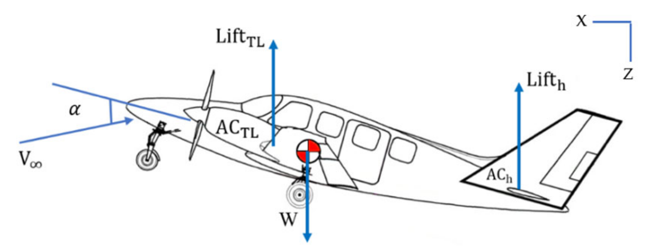
2.1.1. Longitudinal TSC

As shown in Equations (1) and (2), the airplane is considered to be in longitudinal trim when the summation of all forces in the x -direction, including drag and thrust, is zero, and the summation of all moments about the y -axis, including pitching moment, is zero [53]:
F x = 0
M CG = 0
In this study, four disciplines were considered to size the aircraft empennage: aerodynamics, stability and control, propulsion, and weight and balance. For longitudinal TSC, using the MAPLA software package [54,55,56,57], vertical forces were modelled for different aerodynamic and stability characteristics including propwash. As shown in Figure 2, the tailless aircraft configuration creates a lifting force, Lift TL , which is located at the aerodynamic center of AC TL . As the aircraft CG is usually located aft of the aerodynamic center of the main wing, this lifting vector typically generates a positive moment about the CG which causes the aircraft nose to pitch up. For stable flight, the net moment must become zero by employing an upward force behind the CG. The horizontal stabilizer is used to provide this lifting force [48,49,50,51,52,53].
The use of the trim equation leads to Equation (3) as follows [53]:
M CG = M TL + M h = 0
where M T L is the pitching moment generated by the tailless aircraft, which was calculated using the MAPLA software to model the wing, fuselage, nacelle, and propeller effects. M h is the horizontal tail contribution to pitching moment, which accounts for the propeller effects and downwash contribution on the horizontal tail. Equation (3) was nondimensionalized as follows:
C m CG = C m TL η h V H C L h p = 0
where C m T L is the tailless aircraft pitching moment coefficient and C L h p is lift coefficient of the horizontal tail. η h is the tail efficiency factor and is defined as a square of the effective airspeed at the horizontal tail over the aircraft airspeed. V H is the volume coefficient of the horizontal tail and can be expressed using Equation (5) as follows:
V H = S h l h S c ¯
where S h is the horizontal tail area, l h is the distance from the A C h to the CG, and S is the surface area of wing [53].
As longitudinal stability deals with the angular motion of the aircraft, the pertinent dynamic characteristic is the change of the pitching moment, M , with respect to the angle of attack, α . Hence, as shown in Equation (6), the primary stability derivative used to model the static longitudinal stability is the rate of change of the pitching moment coefficient with respect to the change in α , denoted here as C m α . Moreover, with respect to Equation (7), the primary stability derivative that affects the dynamic longitudinal stability is the rate of change of C m with respect to the change in pitch rate, q , presented here as C m q [53]:
C m α = C m α
C m q = C m q

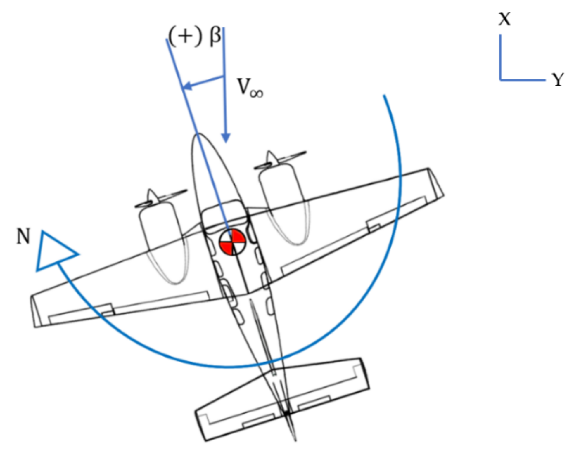
2.1.2. Directional TSC
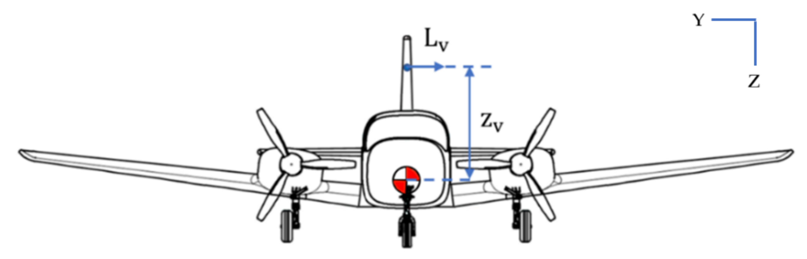
With respect to Equations (8) and (9), the airplane is defined to be directionally trimmed when the summation of all forces in the y -direction and all moments about the z -axis are equal to zero, including the effects of side forces and the yawing moment [53]:
F y = 0
N CG = 0
To model and ensure lateral-directional TSC, the rightward and leftward forces, along with propeller effects, were estimated using MAPLA. In considering directional behaviour, equilibrium refers to a rotational equilibrium for yawing motion, where yaw is defined to occur when the nose of the airplane is pointed away from the flight path within the xy -plane. As shown in Figure 3, the sideslip angle β is used to represent this deviation from the flight path. This can be induced by a crosswind and to offset this angle, a moment N must be generated by the vertical tail. Unlike longitudinal trim where the airplane will be in equilibrium at a range of α , directional equilibrium is often at no sideslip, where β equals zero [48,49,50,51,52,53].
To maintain directional trim, a force in the y -axis must be developed by the vertical tail, which generates a yawing moment. The resulting sum of moments can be expressed as:
N CG = N TL + N v = 0
where N TL is the tailless aircraft yawing moment including wing, fuselage and nacelle contribution calculated using the MAPLA software package. N V is the vertical tail contribution to the total yawing moment, with propeller effects and sidewash contribution accounted for. Equation (10) can be nondimensionalized and expressed as follows:
C n = C n TL + V V C L v p = 0
where C n TL is the tailless aircraft yawing moment coefficient, and C L v p is a lift coefficient of the vertical tail where both consider propeller effects. V V is the volume coefficient of the vertical tail and can be calculated using Equation (10) as follows:
V V = S v l v S c ¯
where S v is the vertical tail surface area, and l v is the distance from aerodynamic center of the vertical tail to the aircraft CG [53].
For multi-engine aircraft, the vertical tail must be designed to stabilize the yawing moment produced during one engine inoperative (OEI) operation. The vertical tail must also be sized for the spin recovery. In the case of multi-engine airplanes, however, spin recovery is not specifically considered as the aircraft are not likely to enter this situation [48]. Hence, Equation (10) can be expressed as follows for the OEI condition:
C n = C n TL + C T R Y T + V v C L v p = 0
where C T R is the right engine thrust coefficient and Y T is the distance between the thrust line and the aircraft CG within the xy -plane [53].
As the directional stability investigates the aircraft’s yawing motion, the corresponding pertinent dynamic characteristic is the change of the yawing moment, N , with respect to the β . Hence, with respect to Equation (14), the primary stability derivative to model static directional stability is the rate of change of the yawing moment coefficient, C n , with respect to the change in the sideslip angle, denoted here as C n β . Furthermore, with respect to Equation (15), the primary stability derivative that informs the dynamic directional stability is the rate of change of C n with respect to the change in the yaw rate, r , and denoted here as C n r [48,49,50,51,52,53]:
C n β = C n β
C n r = C n r

2.1.3. Lateral TSC

With respect to Equations (16) and (17), the airplane is said to be in a state of lateral trim when the summation of all forces in the z -direction and all moments about the x -axis is equal to zero. These considerations include the lift, weight, and rolling moment experienced by the aircraft [53]:
F z = 0
L CG = 0
In Figure 4, the front view of an aircraft is shown where the vertical tail is generating a counteracting moment as a response to the tailless aircraft developing a rolling moment from a nonzero sideslip angle. An additional moment is generated by the rotating propellers, which is also counteracted by the vertical tail. As with directional trim, lateral equilibrium is usually present at a condition with no sideslip, where β = 0 [48,49,50,51,52,53].
To maintain lateral trim, the vertical tail must generate a moment about the x -axis ( L v ), which is equal in magnitude to the rolling moment generated by the tailless body. Thus, the lateral trim equations can be expressed as follows:
L CG = L TL + L V
where L TL is the tailless aircraft rolling moment calculated by MAPLA, which includes the wing, fuselage, nacelles, and propeller contributions. L V is the vertical tail contribution to the total rolling moment, which also contains propeller and sidewash effects. Equation (18) can be nondimensionalized and expressed as follows:
C l = C l TL + S V z V S c ¯ C L V p = 0
where z V is the distance from the AC of the vertical tail to the aircraft CG [53].
As lateral stability is concerned with the aircraft’s rolling motion, the corresponding pertinent dynamic characteristic is the change of the rolling moment, l , with respect to the sideslip angle β. With respect to Equation (20), the primary stability derivative to calculate the static lateral stability is the rate of change of yawing moment coefficient, C l , with respect to the change in the sideslip angle, denoted here as C l β [48,49,50,51,52,53]:
C l β = C l β
More information is available in the flight dynamics books by Roskam [58], Nelson [59] or Etkin [60].

2.2. MAPLA

The enhanced semi-empirical multidisciplinary analysis program MAPLA was used to model the relevant disciplines. This tool is specifically built for design optimization of light, general aviation, propeller-driven aircraft, and includes analyses for four disciplines: aerodynamics, propulsion, performance, as well as stability and control. MAPLA includes state-of-the-art analytical procedures and design data collections, which have been combined and modified in a unique method, which is fully automated. Previous investigations demonstrated that MAPLA was able to determine the aerodynamic characteristics of light aircraft with an acceptable accuracy in various configurations [54,55,56,57]. While this program performs well in modelling light general aviation aircraft with conventional configuration, which was the focus of its development, the module’s use of semi-empirical methods has the unfortunate consequence of it not being generally applicable. For the purposes of this investigation, where a conventional light aircraft was targeted, MAPLA was more than sufficient.

2.3. PBDO Method Outline
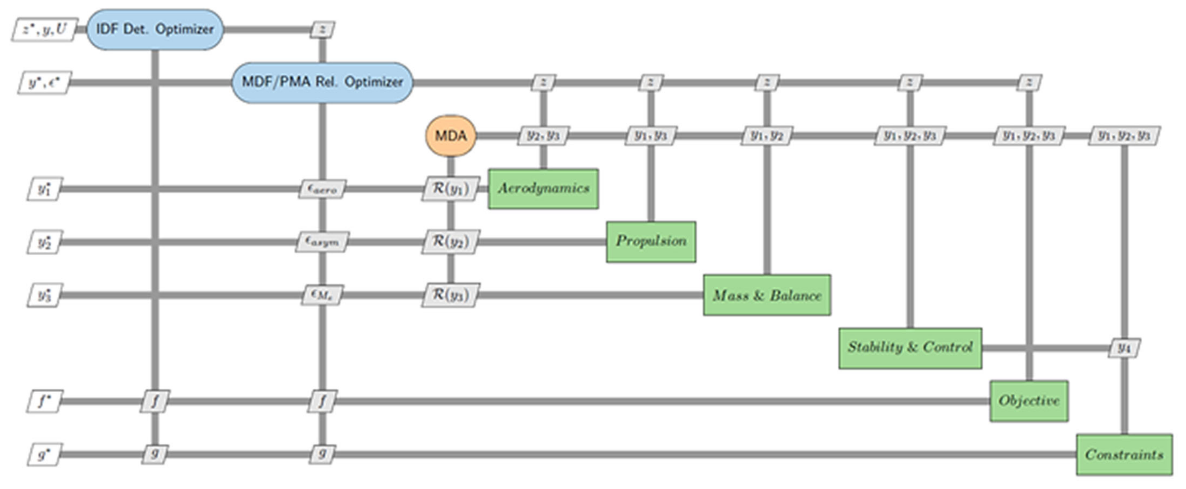
The optimization algorithm contains a deterministic optimizer which works sequentially with a possibility–evaluation algorithm. This framework is comparable to the Sequential Optimization and Reliability Assessment (SORA) procedure developed for RBDO [61,62]. The Performance Measure Approach (PMA) was used to implement the possibility evaluation on each constraint, which was followed by a deterministic optimization. The PMA algorithm consists of a separate optimization loop which finds a worse-case scenario for each constraint separately. The position of each uncertain variable and parameter within their intervals are determined such that that the constraint is maximized. This guarantees that constraints will be satisfied even in the extreme worst-case where each individual source of uncertainty drives the designs towards constraining limits [63,64]. A Sequential Quadratic Programming (SQP) procedure is used in both the deterministic optimization and the PMA-based possibility evaluation. The method accomplishes deterministic optimizations in sequence with possibility evaluations, altering the constraints until convergence can be guaranteed [65].
To validate the MDO framework, the following nonlinear single-discipline RBDO test problem was solved with different methods, after which the results were compared [65,66]:
min f = x ¯ 1 + x ¯ 2 st .   P G j x 0 P goal ,   j ,   j = 1 , 2 , 3 G 1 x = x 1 2 x 2 20 1 G 2 x = x 1 + x 2 5 2 30 + x 1 x 2 12 2 120 1 G 3 x = 80 x 1 2 + 8 x 2 + 5 1 x 1 ~ N x 1 , 0.3 ,   x 2 ~ N x 2 ,   0.3
The problem was solved for the constraint boundaries of G 1 , G 2 , and   G 3 with different reliability indices β r of 1 to 5 with the double loop method using Reliability Index Approach (RIA) and PMA, the sequential method with PMA, and the single-loop method [65]. The algorithm performance was compared at β r = 3 for all methods and is shown in Table 1 as follows:
It was found that the double loop and sequential methods all yielded approximately equal results but required varying numbers of evaluation to arrive at these results. As shown in Table 1, the PMA-based methods solve required fewer evaluations and by extension fewer computation resources. Of the two PMA methods, the sequential implementation was noted to require less function evaluations than the double loop approach. For this problem, the single loop approach was found to need the smaller number of evaluations but demonstrated a divergence from the PMA and RIA methods when β t was increased.
The stability, speed, and accuracy of each method, shown in Table 2, were also evaluated by running the optimization over a grid of 100 points between [0;0] and [10;10].

3. MDO Framework

3.1. Methods

MDO methods are classified into tw7o different categories: single-level and multilevel methods. Of the seven methods mentioned prior, MDF, IDF, AAO, SAND and MDOIS are categorized as single-level methods which implement a single optimizer and directly use a non-hierarchical structure. The remaining methods are the multilevel methods: CSSO, BLISS and CO. For the single-level methods, with the exception of the MDOIS approach, coupling variables are updated by the individual disciplines within a global iteration. The MDOIS approach only updates these coupling values after all disciplines have finished computation and a global multidisciplinary analysis is run. In considering the multilevel methods, the core difference is that the architectures include a hierarchical structure with a separate optimizer at each level [32].
In this paper, the RyeMDO IDF/Sequential/PMA framework with an SQP optimization algorithm has been implemented. A framework was developed which implements a PBDO algorithm to find the optimum empennage design configuration for the twin-engine propeller driven aircraft. The algorithm consists of a PBDO solver coupled with MAPLA to provide the four analyses. In the previous work [65], this framework was found to be reliable and less dependent on constraint functions and coarse objectives than the double loop procedures. Moreover, this framework was shown to have a smaller dependency on the starting vector selection compared with the single loop procedure, whilst being more effective than all methods save for the single loop approach in the considered cases. The sequential approach was chosen as it provides more benefits when solving for multi-level reliability [65].
The sequential framework resolves a sequence of deterministic optimizations first, then carries out reliability evaluations until convergence is achieved. This results in the intermediate solutions gradually passing through lower indices until the target level is reached [65]. In this work, the low reliability index was applied at the first step and then gradually higher indices were used. This allows the approach to extract intermediate answers and plot the connection between the optimal design and nominated target reliability index without significantly increasing the number of function evaluations. The objective function was defined to minimize the empennage package weight for the specified flight conditions while lowering the reliability index of the designs.
In this paper, for the reliability assessment sub-problems, the MDF approach was selected instead of the IDF method. This was justified on the grounds that, for problems with a large number of variables and fewer uncertainties, the dimensionality of the reliability analysis is significantly larger in the IDF framework. Moreover, the auxiliary equality constraints had to be considered for coupling variable consistency, producing significant complexity in the outcome that must be solved for every constraint in each iteration of the sequential procedure. By using the MDF approach for reliability assessments, the dimensionality of the PMA optimization was reduced and no auxiliary constraints had to be considered. In previous work [65], it was shown that the PMA reliability evaluations converged sooner for the MDF approach and with higher reliability.
With respect to the four different disciplines considered in this study (aerodynamics, propulsion, mass and balance, as well as stability and control), the XDSM flowchart in Figure 5 is presented for the multi-disciplinary optimization procedure of the twin-engine propeller-driven aircraft. To run the system-level optimizer, each sublevel was analyzed sequentially with the output of one discipline providing input to another. Using this approach, the empennage surface area was optimized based on the geometric parameters and the corresponding flight condition achieved by each discipline. The method is outlined as follows and the corresponding block diagram is shown in Figure 5:
1.
Find the analysis error distributions
(I)
Model each entry based on the aircraft empennage model
(II)
Determine the entire aircraft aerodynamic characteristics
(III)
Implement the uncertainty analysis
(IV)
Implement a best fit PDF curve for each individual source of uncertainty
2.
Choose the starting vector and a list of reliability indices
3.
Run the IDF-based deterministic optimization
4.
Run the MDF-based PMA reliability evaluation at the current reliability index, and alter variables according to the sequential procedure
5.
Check for convergence with current reliability goal
(I)
if yes, update starting vector with the current optimum point, select next reliability goal, return to 3
(II)
if no, return to 3
6.
Advance to next target reliability level
(I)
retain solution as new starting vector
(II)
return to 3

3.2. Disciplines

Four disciplines of analysis were considered in this investigation. The first of which was the aerodynamic analysis, which consists of longitudinal and lateral-directional aerodynamic coefficients and stability derivatives. Power-off aerodynamic coefficients are initially estimated for each section of the tailless aircraft, including the wing, fuselage and nacelle. The empennage package is subsequently introduced to consider the horizontal tail, vertical tail and high-lift surface contributions. Following this, the static stability derivatives are calculated and the total power-off characteristics are obtained through combining the contributions of each aircraft part. Afterwards, the dynamic stability characteristics of the aircraft are estimated by using the stability derivatives. Finally, the power-on parameters and propeller effects were added to the estimations through the use of semiempirical methods.
After the aerodynamic analysis concludes, the weight of each component is calculated through a statistical method based on the MIL-STD-1374 via a “Summary Group Weight Statement” [18,68,69]. Both the mass and CG of individual components are calculated by statistical equations to provide the overall empty weight of the airplane [18,68,69].
Aircraft handling quality is evaluated using the flying quality subprogram of MAPLA. This module enables the estimation of the aircraft trim characteristics in all flight and aircraft configurations, thereby providing the corresponding handling quality level for different longitudinal and lateral-directional modes in accordance with the standards of this aircraft type.

3.3. Design Variables

As this study’s main concern was to size the empennage of a twin-engine propeller-driven light aircraft, the corresponding design variables were selected based on the effectiveness of each component with respect to the semi-empirical method estimations. These variables are shown in Figure 6. In addition to the tail components, the engine placement was also parametrized due to the impact on rudder design. The engine position is represented as the lateral position on the wing, measured as a y -direction distance from the x -axis. The full list of design variables is shown in Table 3.

3.4. Objective Functions

Two scenarios are considered for the objective function. For the first scenario, the weight optimization was investigated and, for the second scenario, the optimization targeted the minimum drag in a trimmed flight condition. In the following, both scenarios were described and the corresponding results are shown in Section 4.
For the first scenario, the objective function for the optimization process is to minimize the weight of the horizontal and vertical stabilizers by varying the design variables shown in Table 1. The resulting equation has a direct relation with the surface areas of the horizontal and vertical tail, which allows the optimization scheme to produce a design with minimal area.
The horizontal tail weight, W h , was estimated with a statistical relationship provided for the general aviation aircraft type using Equation (22) as follows [17]:
W h = 0.016 N z W d g 0.414 q 0.0168 S h 0.896 100 t c h cos Λ   c ¯ 4 h 0.12 AR h cos 2 Λ   c ¯ 4 h 0.043 λ h 0.02
where N z is the ultimate load factor and is equal to 1.5 times of aircraft load factor limit, q is the dynamic pressure ratio, W d g is the flight design gross weight, t c h is the horizontal tail airfoil section thickness ratio, Λ   c ¯ 4 h is the sweep angle of the horizontal tail at ¼ of the mean aerodynamic chord, AR h is the aspect ratio of the horizontal tail and λ h is the taper ratio of the horizontal tail.
The surface area of the horizontal tail was calculated using Equation (23) based on the geometrical parameters provided in Figure 6 as follows:
S h = c r h b h c e h for b h 2 c e h back b h 2
where c e h for is the extended panel out of the tip chord of the horizontal tail and can be found in Figure 6 using the trailing edge angle of the horizontal tail as follows:
c e h for = b h 2 tan Λ LE h
In addition, c e h back can be calculated using the
c e h back = b h 2 tan Λ TE h
where Λ TE h is the trailing edge sweep angle of the horizontal tail and can be found using Equation (26) as follows:
Λ TE h = 90 arctan b h 2 c r h c t h c e h for
Following this, the vertical tail weight, W v , was calculated using the following statistical equation [18]:
W v = 0.073 1 + 0.2 z h z v N z W d g 0.376 q 0.122 S v 0.3873 100 t c v cos Λ   c ¯ 4 v 0.49 AR v cos 2 Λ   c ¯ 4 v 0.375 λ v 0.039
where t c v is the vertical tail airfoil section thickness ratio, Λ   c ¯ 4 v is the sweep angle of the vertical tail at one quarter of the mean aerodynamic chord, AR v is the aspect ratio of the vertical tail and λ v is the taper ratio of the vertical tail.
Similarly, the surface area of the vertical tail was computed using the following equation, which was again based on the geometrical parameters provided in Figure 6:
S v = c r v c t v + c e v b v 2 + c t v b v b v 2 tan ϕ TE 2
where c e v is the extended panel out of the root chord of the vertical tail and was found with the trailing edge sweep angle as follows:
c e v = b v tan ϕ TE
For the second scenario, MAPLA’s stability and control module was used during the optimization process to find the trim condition and its corresponding drag force, which was used as an objective function to be minimized.

3.5. Constraints

First and foremost, manufacturing constraints were employed in defining the lower and upper limits for each design variable. The total empty mass of the aircraft was considered to be below 2000 kg according to statistical data and an initial weight and balance analysis. Static and dynamic criteria were also set as the constraints in the optimization process. The effectiveness of the control surfaces during cruise and climb-out were evaluated to ensure acceptable pitch authority as achieved in slow flight and that yaw authority was maintained in single-engine flight.
To have longitudinal static stability, C m α must be negative. The typical value for most airplanes is between –0.3 to –1.5 1/rad. For longitudinal dynamic stability, the real part of the roots of the longitudinal characteristic equation must be negative. A major contributor to this criterion is C m q , such that a negative value has a robust stabilizing effect. The typical value of C m q for most airplanes is between –5 to –30 1/rad [53]. Additionally, longitudinal stability was constrained to a static margin of 5%.
To achieve roll stability, the value for C l β must be negative [48]. Furthermore, to maintain directional static stability, C n β must be positive. The typical value for most airplanes is around +0.1 to +0.4 1/rad. For directional dynamic stability, the real part of the roots of the lateral-directional characteristic equation must be negative. A major contributor to this criterion is C n r , such that a negative value has a robust stabilizing effect. The typical value for most airplanes is about –0.1 to –1 1/rad [53]. Yaw static stability must be ensured for a full-thrust climb scenario with one failed engine. The constraint ensures that the rudder and vertical tail have acceptable authority. All these constraints are considered in the optimization algorithm [70,71,72,73].
In addition, airworthiness requirements for light aircraft, particularly from CS-23 and available information from military standards for dynamic modes, were set as the constraints in the optimization process. The corresponding constraints for each mode were discussed in the Results section. The list of all constraints is provided in Table 4 as follows.

3.6. Sources of Uncertainty

The uncertainty due to the use of semi-empirical approaches in the aerodynamics and stability disciplines are somewhat difficult to measure. However, recent computing power enhancements can provide an answer with ~80% accuracy using the initial structure given by the initial aircraft layout [74]. From this, the error term was assumed to be uniformly distributed between the highest and lowest observed error. The error term was defined as the ratio of predicted characteristics to the observed characteristics from the database, ε aero . The characteristics from the aerodynamics discipline was then scaled by this ratio to correct for this error as shown in Equation (30). The error term was taken to be a uniformly distributed random parameter:
ε aero = aero characteristics p aero characteristics aero characteristics = ε aero aero characteristics p
The designs from the compiled aircraft database were modeled and the predicted empty-mass of each design was compared with the observed value from the database. The histogram of the errors indicated that the empty-mass error term could be approximated by a normal distribution curve. The mass error term was defined as shown in Equation (31). Empty-mass calculations carried out by the optimizer were scaled by the error term to account for the uncertainty in the prediction of the aircraft empty mass:
ε M e = M e p M e db   M e = M e p ε M e
Furthermore, a previous study [56] showed that the required rudder deflection in OEI scenarios could be signified due to the asymmetric blade effect of propellers. It was shown that a maximum of 4 degrees of rudder deflection was expected to be considered in the design of the rudder surface for light aircraft. Accordingly, rudder deflection error was approximated by considering the asymmetric blade thrust effect. The propeller effect error term was defined in Equation (32) as follows. Maximum rudder deflection calculations carried out during the optimization process were scaled by the error term to account for the uncertainty in the prediction of the required rudder deflection:
δ r max = ε asym δ r max p

4. Results

In this section, the resulting geometry of the optimized empennage configuration, as well as the aerodynamic characteristics and dynamic stability of the twin engine propeller driven aircraft, are shown for both aforementioned objective scenarios.

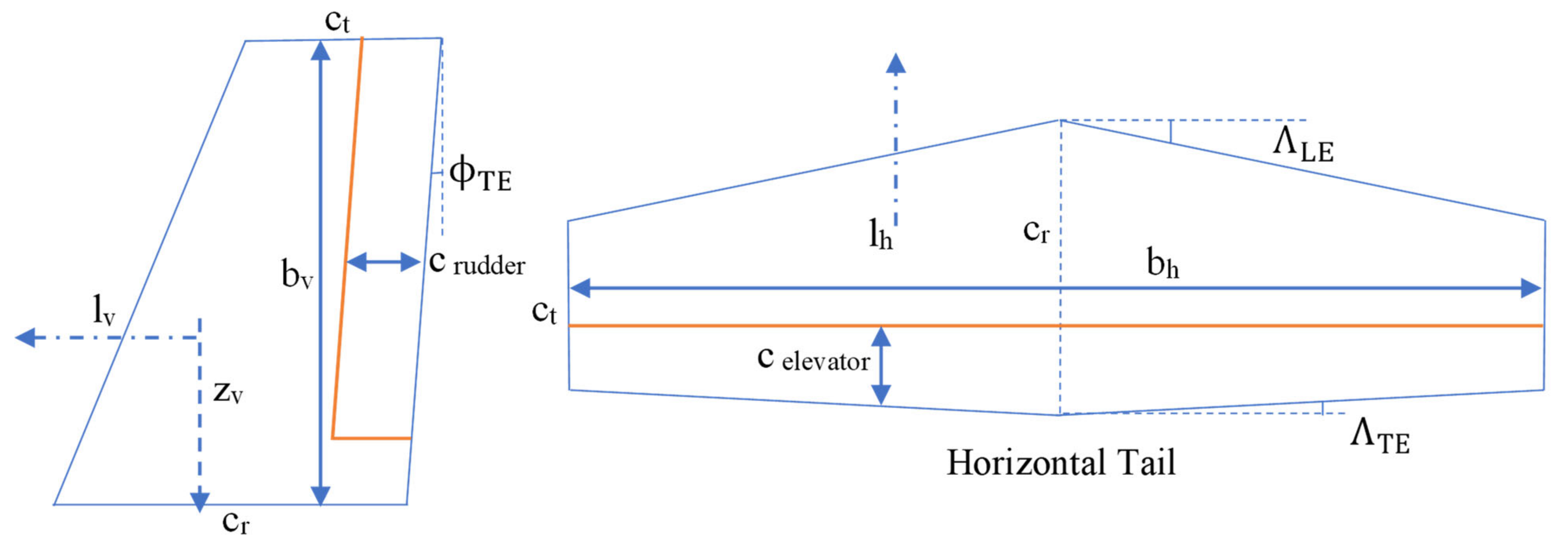
4.1. Resulting Geometry

After running the optimization algorithm, the resulting geometry for the empennage configuration, considering the aforementioned objective scenarios, constraints and uncertainties, is shown in Figure 7a and the complete aircraft can be seen in Figure 7b, produced with MAPLA’s geometry module. The corresponding variables results were also presented in Table 5. As can be seen, the resulting aircraft empennage sizing using both scenarios of mass minimization and the drag optimization in trim flight were similar.

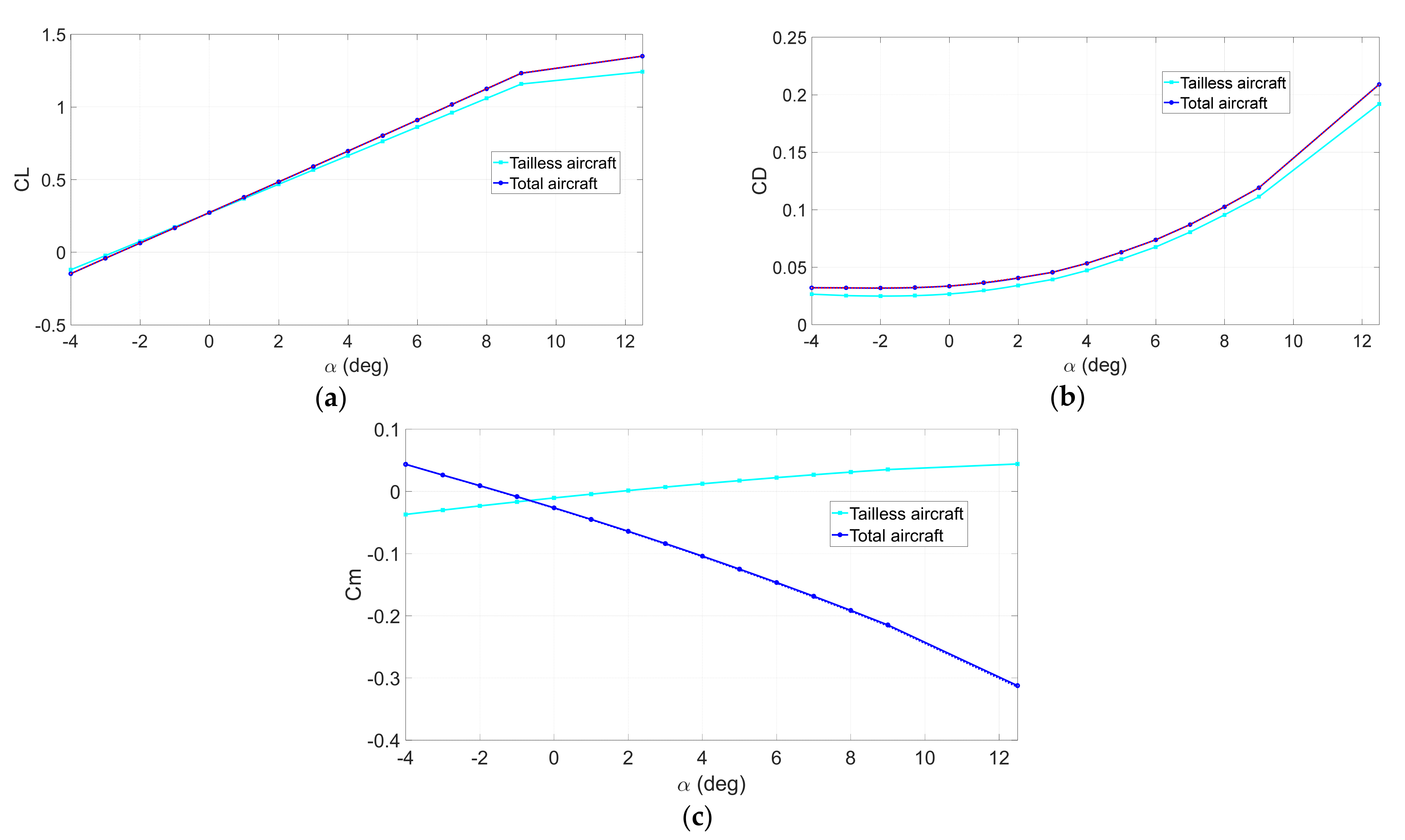
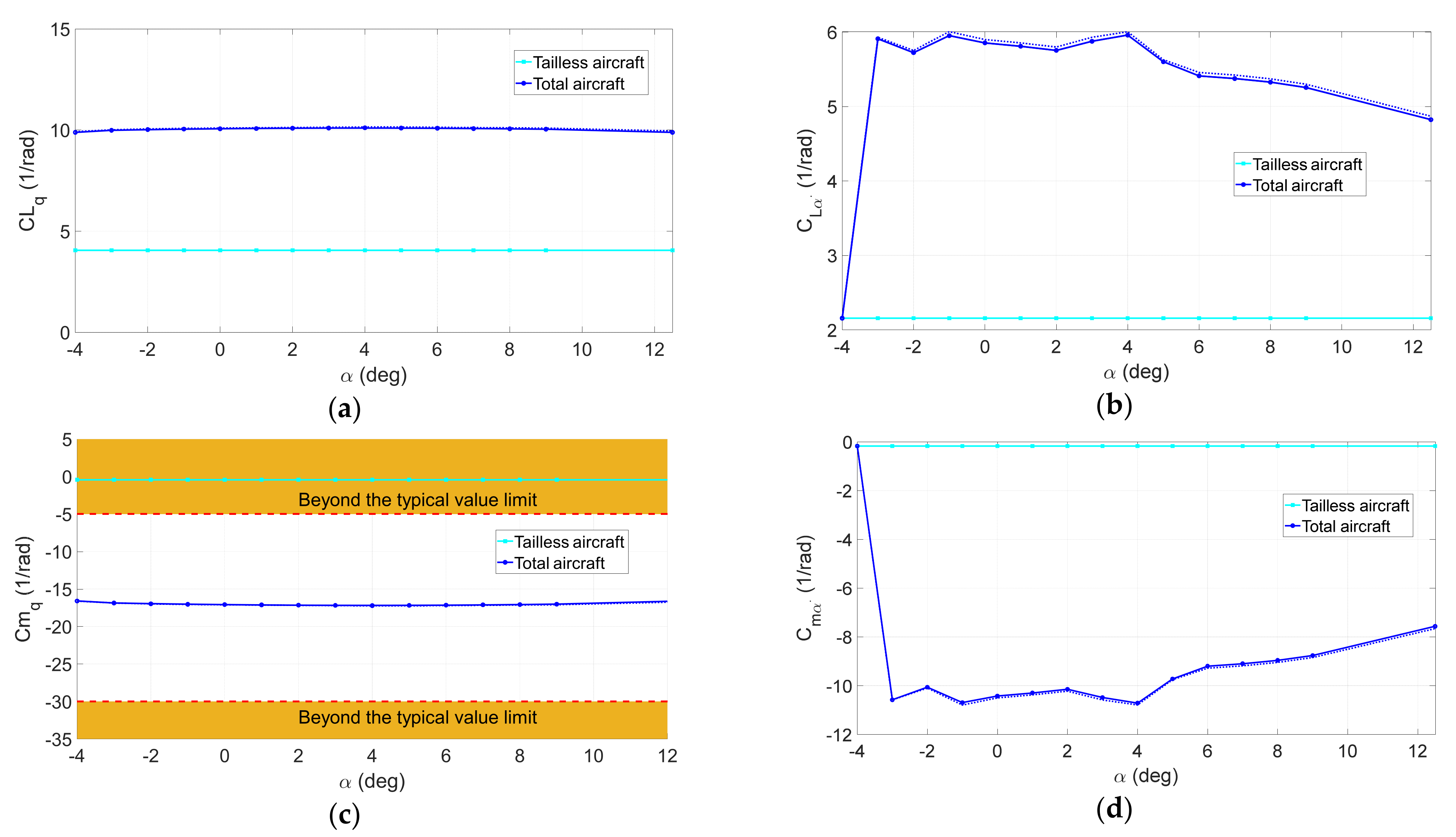
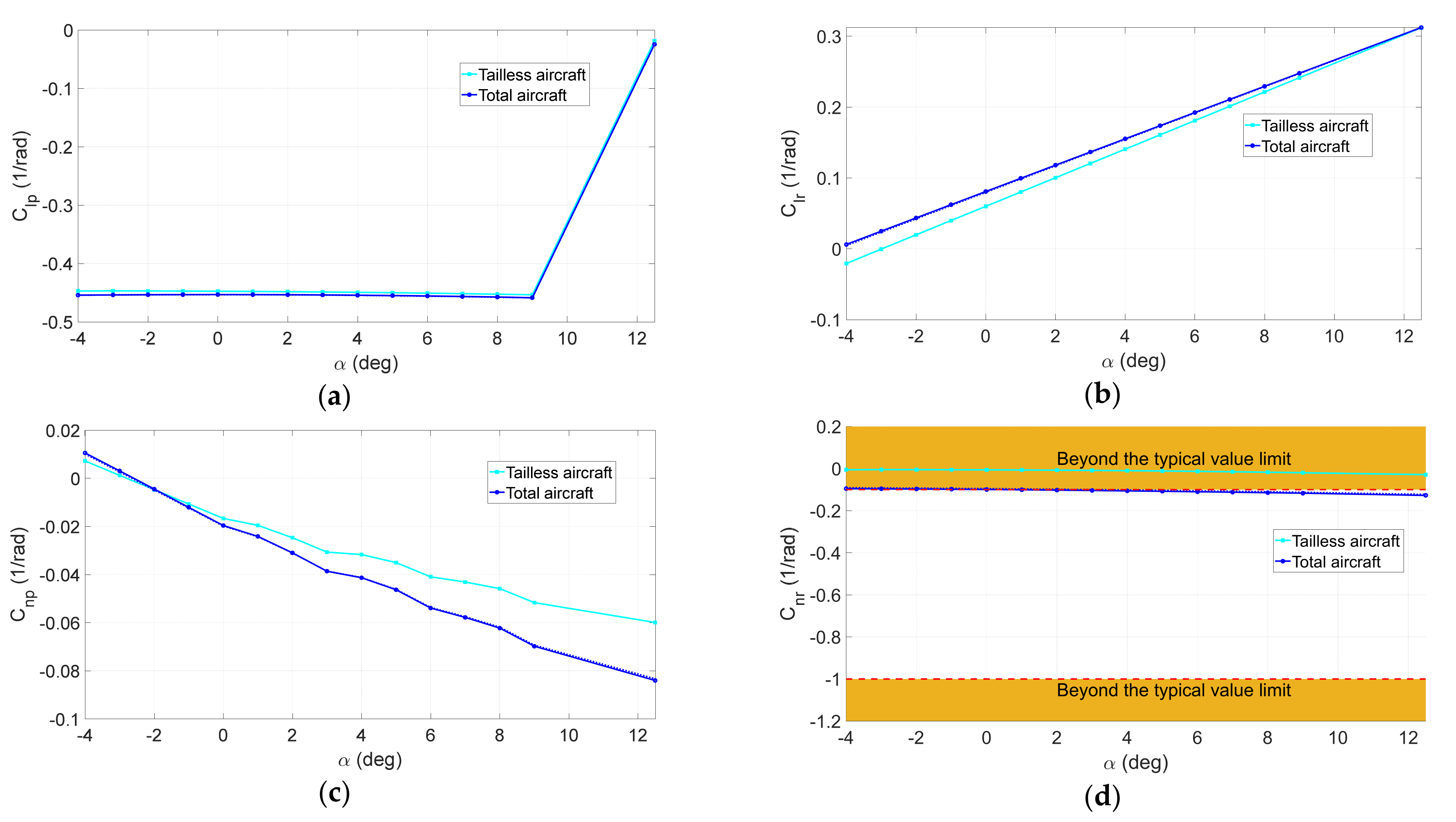
4.2. Aerodynamics Characteristics of the Optimized Aircraft

MAPLA’s aerodynamics characteristics were compared with experimental data for a twin-engine light general aviation aircraft provided by NASA with similar characteristics to the one studied here [75,76]. Moreover, MAPLA has been used for design optimization of similar single and twin-engine propeller-driven light aircraft (e.g., two-, four- and six-seat propeller driven aircraft) [54,55,56,57]. The results demonstrated that MAPLA was able to determine the aerodynamic characteristics of the light aircraft with an acceptable accuracy. Aerodynamic characteristics of the aforementioned twin-engine aircraft are shown in the cruise flight condition, using the optimized tail model developed by implementing the proposed multidisciplinary possibilistic approach. The dotted-line results presented in the following figures are representative of the case with the drag optimization scenario.
Figure 8 shows the longitudinal static characteristics for both the tailless and whole aircraft configurations. As demonstrated in Figure 8c, the total aircraft configuration provided a value of approximately –1 1/rad for C m α using the optimized tail configuration, which matches best within the typical value range discussed previously of 0.3 C m α 1.51 / rad . In addition, a small positive value for the C m 0 was expected, which in this case was equal to 0.05. As can be seen from the results shown in Figure 8, both optimization results show the same behavior.
Figure 9 shows the lateral-directional static characteristics for both the tailless and total aircraft configurations. As can be seen in Figure 9c, the complete aircraft configuration provided a value of about 0.12 1/rad for C n β using the optimized tail configuration which aligns with the typical value range discussed earlier of 0.1 C n β 0.41 / rad . In addition, for roll stability, the value for C l β must be negative, and, for this aircraft, it was found to be approximately 0.11 / rad , which was considered acceptable. Similar to the longitudinal characteristics, the results shown in Figure 9 reveal the same behavior for both optimization scenarios with the mass optimization and minimum drag optimization in the trim flight condition.
Figure 10 presents the longitudinal dynamic characteristics for both tailless and total aircraft configurations. As can be seen in Figure 10c, the total aircraft configuration provided a value of approximately –18 1/rad for C m q using the optimized tail configuration, which complies with the typical value range discussed earlier, 5 C m q 301 / rad . Additionally, the results clearly show the proper contribution of the tail configuration in the dynamic stability of the proposed twin-engine aircraft design.
Figure 11 shows the lateral-directional dynamic characteristics for both the tailless and total aircraft configurations. As can be seen in Figure 11d, the total aircraft configuration provided a value of approximately 0.1 1/rad for C n r using the optimized tail configuration, which also lies within the typical value range discussed earlier, 0.1 C n r 11 / rad . Similar to the static aerodynamic characteristics, the results shown for the dynamic characteristics in Figure 10 and Figure 11 reveal the same behavior for both optimization scenarios with the mass optimization and minimum drag optimization in the trim flight condition.

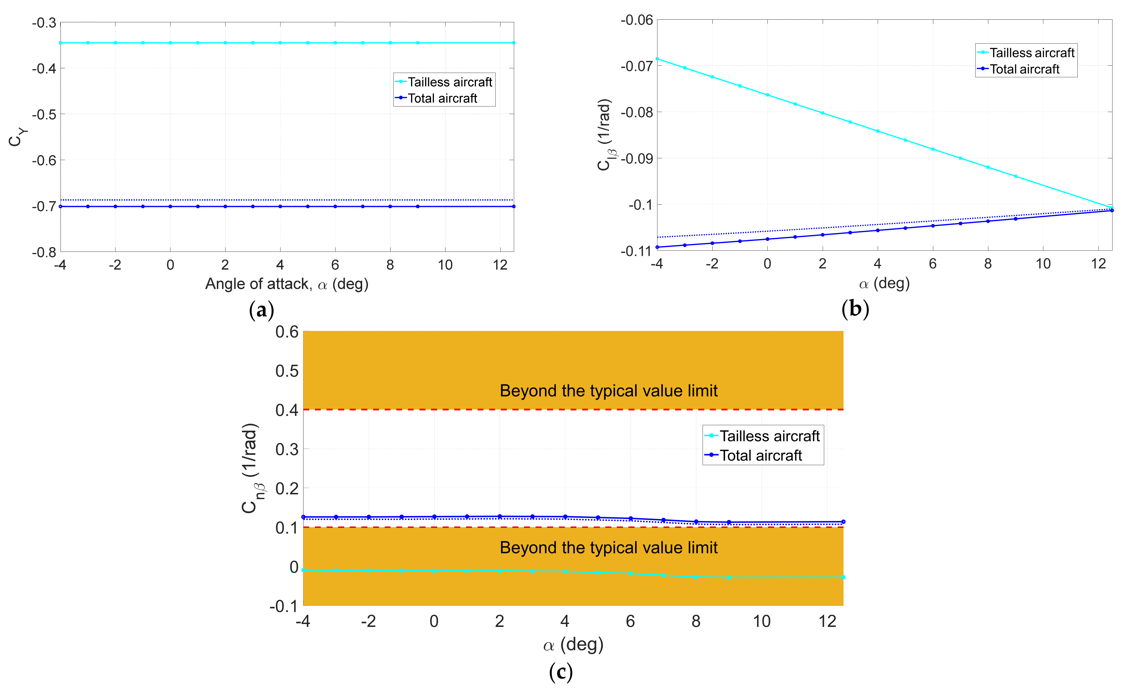
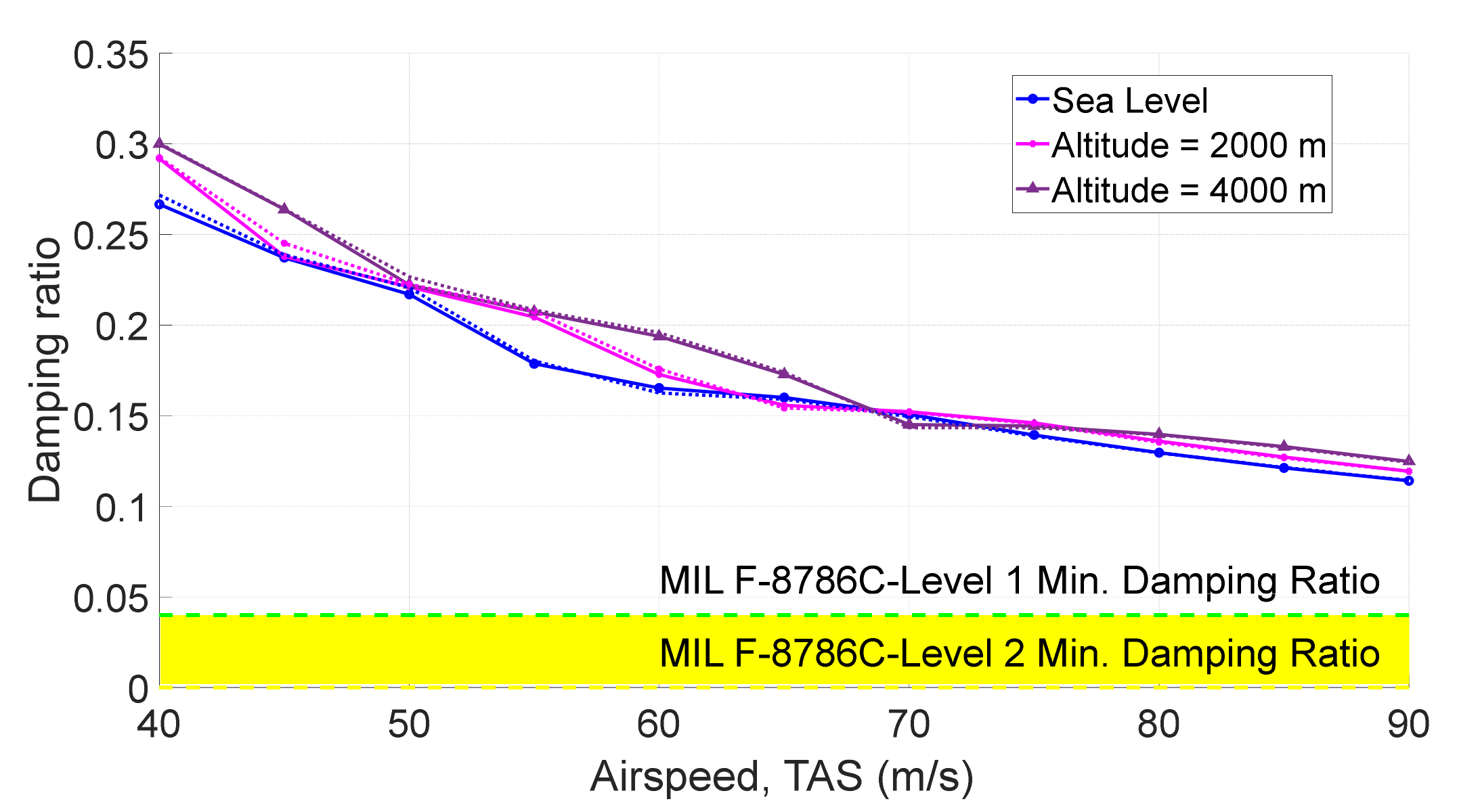
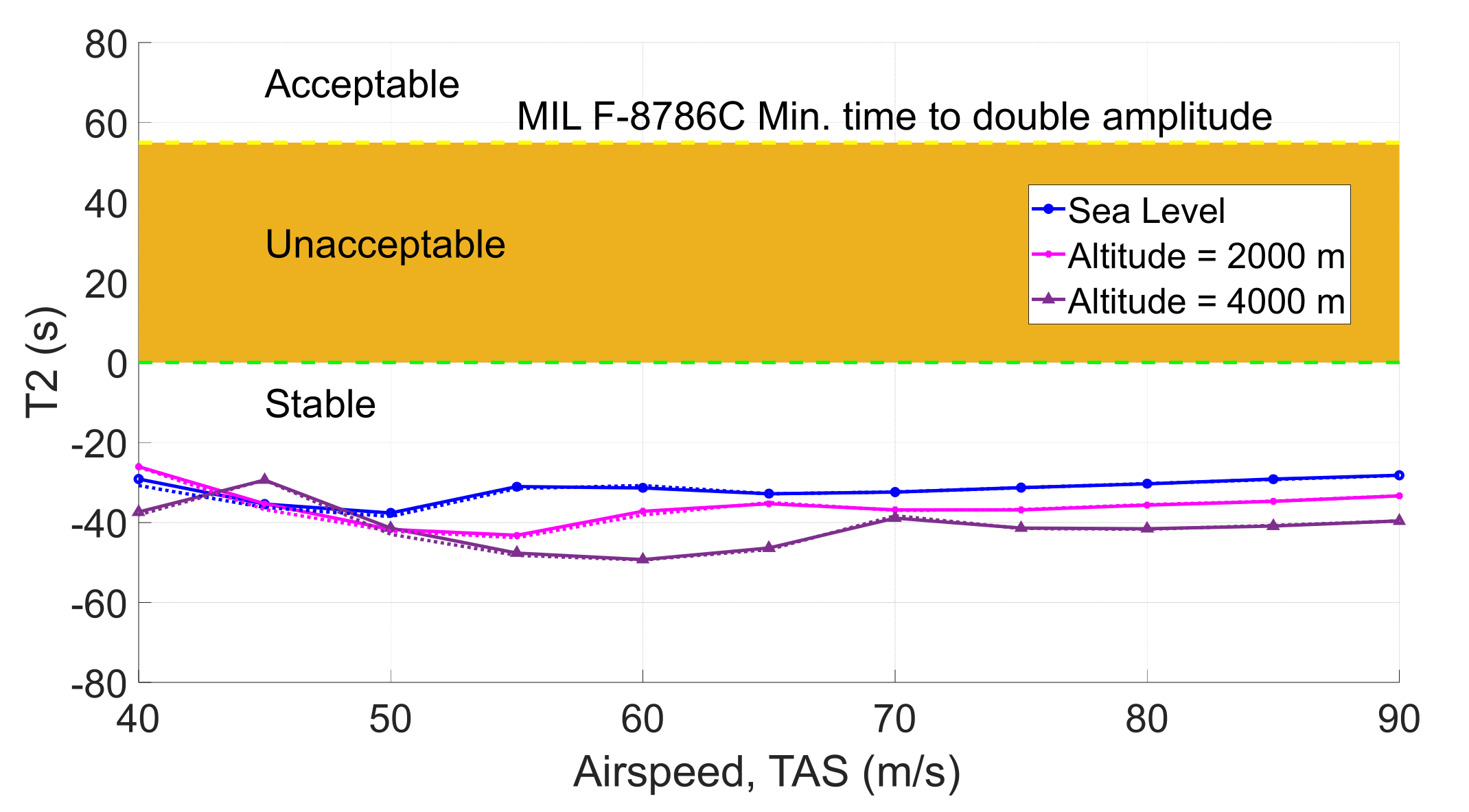
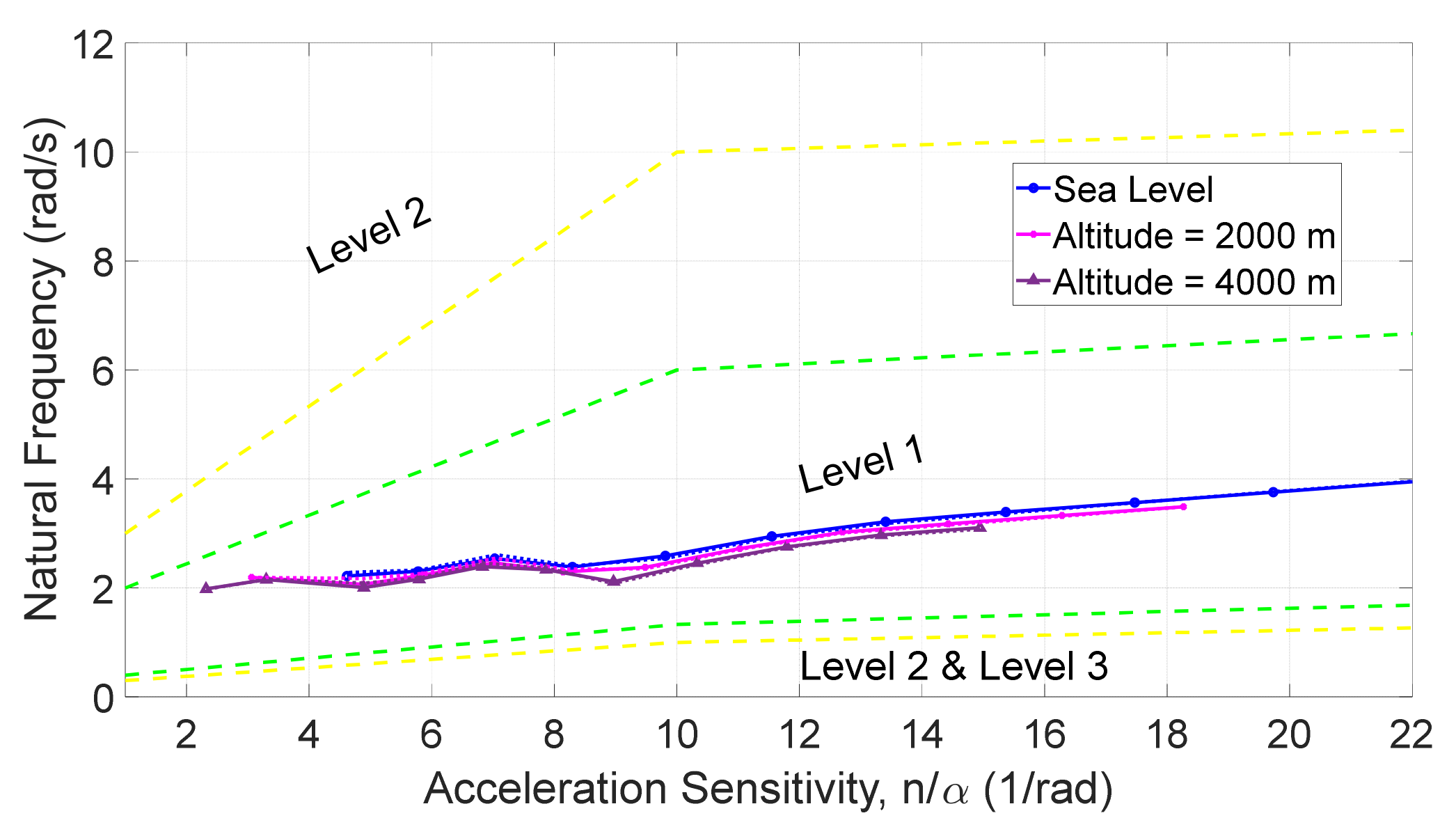
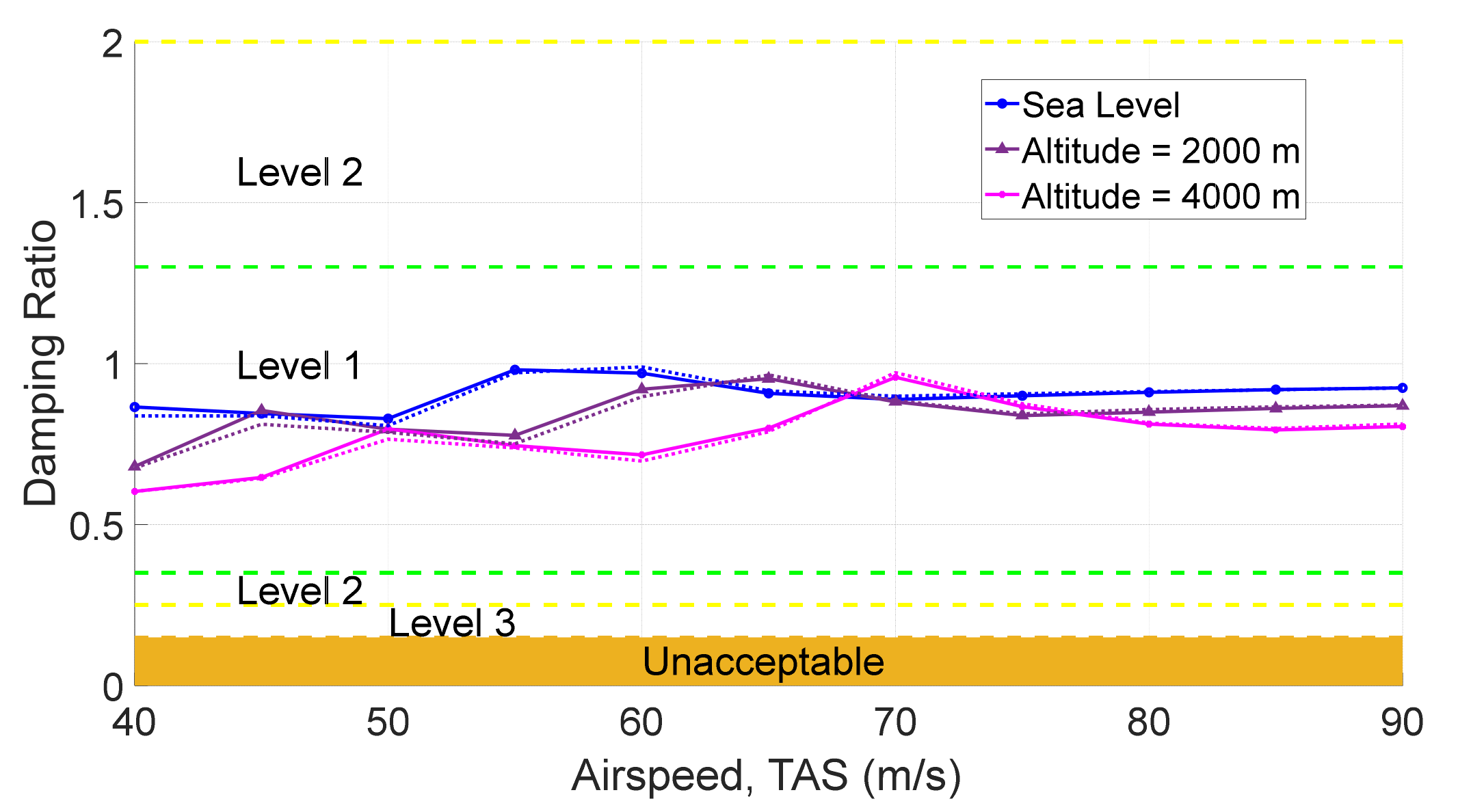
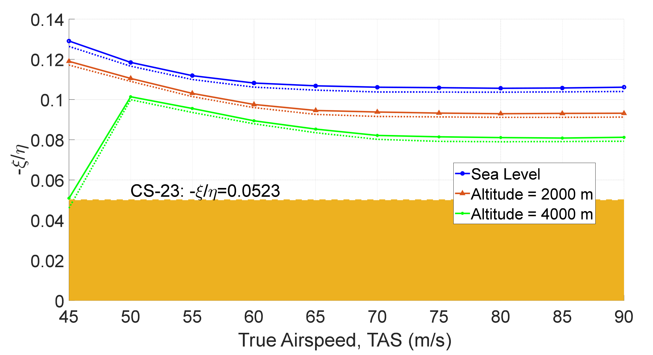
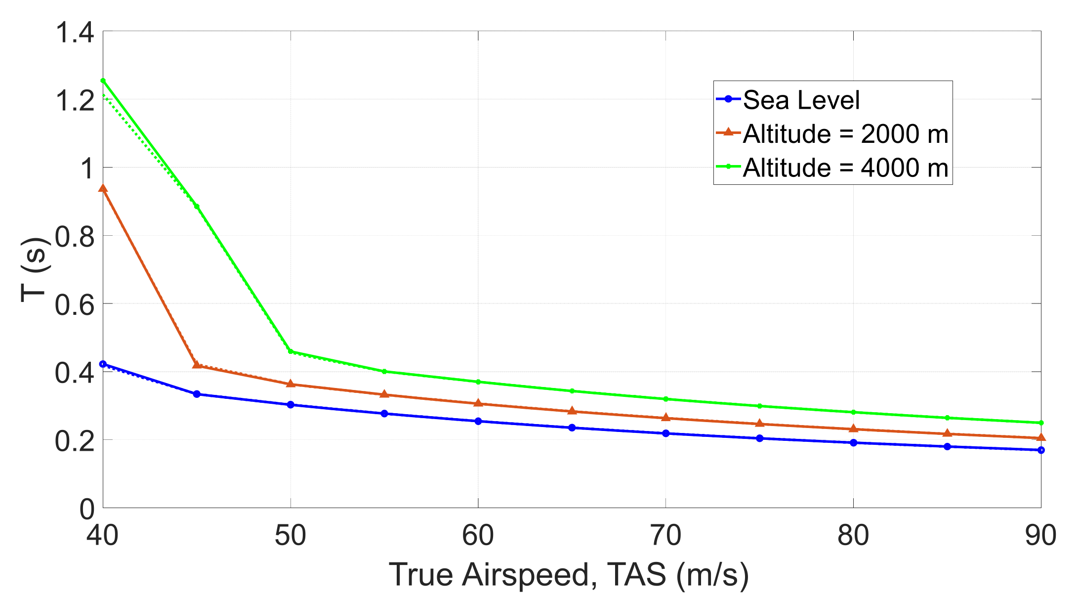
4.3. Flight Dynamic Stability of the Optimized Aircraft

In this section, the results of the dynamic stability analysis obtained for the optimized aircraft are discussed in greater detail to investigate the dynamic stability requirements of the proposed twin-engine propeller driven aircraft. Nearly all periodical modes were stable at the tested airspeeds and flight altitudes. The stability requirements were defined as constraints for the optimization algorithm. The constraints were enforced using an indirect method which imposes a penalty for any cases beyond the boundaries. The penalty does not ensure that constraints are beyond the limits; thus, in a few cases, the boundaries were slightly crossed, but remained within an expected tolerance. In the following, the dynamic mode characteristics are discussed in detail with respect to the airworthiness criteria. The results were obtained for aftmost CG location at the maximum weight.
With respect to the CS-23 airworthiness requirements [74], the phugoid mode was noted to not be particularly strong. In Figure 12, the phugoid mode damping ratio against the MIL criteria has been shown [75,76]. The damping characteristics satisfy the Level 1 acceptance for all range of airspeeds from stall to the maximum cruise speed. Figure 13 shows time to double for the phugoid amplitude. The negative values show that the oscillations are stable.
Figure 14 presents the short period undamped natural frequency versus acceleration sensitivity. As can be seen, the results were inside the envelope of the first acceptance level according to MIL criteria [74]. Figure 15 further shows the damping ratio level for the short period mode, which nicely satisfies the first acceptance level of the CS-23 requirement to be strongly damped. Reprinted from [74].
According to CS-23.181, the Dutch roll requirements were given precisely as: “Any combined lateral-directional oscillations (“Dutch roll”) occurring between the stalling speed and the maximum allowable speed appropriate to the configuration of the aeroplane must be damped to 1/10 amplitude in 7 cycles…”. Figure 16 shows that this criterion has also satisfied the design.
Figure 17 shows the time to double the roll mode amplitude. With respect to Figure 17, the roll mode was strongly damped, which is typical for the most airplanes. The spiral mode characteristics are presented in Figure 18. As can be seen, values for time to double show that the spiral mode is also strongly damped according to CS-23 and MIL-F-8785-C. [72,74]. Complying with both regulations, the spiral mode falls within level 1 of requirements in most cases. For very low speeds near stall speed and at higher altitudes, the spiral mode level may decrease to the level of 2 or 3. At all points, however, the results remain within the acceptable range of the criteria.

5. Conclusions

In conclusion, the proposed multidisciplinary possibilistic approach successfully provides the capability to size the empennage package of a multi-engine propeller-driven aircraft by altering the tail geometry in the early design stages where several uncertainties are present due to low fidelity estimations. In this work, four disciplines were considered including aerodynamics, stability and control, propulsion and weight and balance. Considering various design criteria, including longitudinal/lateral/directional trim, stability characteristics, and other requirements, the optimized tail configuration provided the design with the desired characteristics to ensure that airworthiness requirements were met and predefined constraints were complied with while offering an optimal form. Results showed that the aircraft empennage sizing using both scenarios of mass minimization and the drag optimization in trimmed flight produced very similar configurations. The proposed approach may be used to improve the preliminary design process of multi-engine propeller driven light aircraft.

Author Contributions

Conceptualization, M.R. and J.C; Methodology, M.R., J.B., D.N. and J.C.; Software, M.R.; Formal analysis, M.R., J.B. and D.N.; Writing—original draft, M.R.; Preparation, M.R.; Data curation, J.B. and D.N.; Writing—review and editing J.B., J.C. and D.N. All authors have read and agreed to the published version of the manuscript.

Funding

This work was funded by Mitacs through the Mitacs Accelerate Program (reference number: IT16648) and Columbiad Launch Services Inc.

Conflicts of Interest

The authors declare no conflict of interest.

Nomenclature

Roman Symbols
b h Horizontal tail span
b v Vertical tail span
C L h p Lift coefficient of the horizontal tail
C L v p Lift coefficient of the vertical tail
C l Yawing moment coefficient
C l β Rate of change of yawing moment coefficient with respect to the change in the sideslip angle
C m CG Nondimensionalized moments about the y-axis
C m q Rate of change of the pitching moment coefficient with respect to the change in pitch rate
C m TL Tailless aircraft pitching moment coefficient
C m α Rate of change of the pitching moment coefficient with respect to the change in the angle of attack
C n Yawing moment coefficient
C n TL Tailless aircraft yawing moment coefficient
C n r Rate of change of yawing moment coefficient with respect to the change in the yaw rate
C n β Rate of change of yawing moment coefficient with respect to the change in the sideslip angle
C T R Right engine thrust coefficient
  c ¯ Mean aerodynamic chord
F x ,   y ,   z Forces in the x-, y- and z-direction
fObjective function
Gi Constraint boundary
i h Horizontal tail incidence angle
k Counter used in the optimization process
L CG Moments about the x-axis
L TL Tailless aircraft rolling moment
L V Vertical tail contribution to the total rolling moment
l h Distance from the aerodynamic centre of the horizontal tail to the CG
l v Distance from aerodynamic center of the vertical tail to the aircraft CG
M Pitching moment
M CG Moments about the y -axis
M h Horizontal tail contribution to pitching moment
M T Tail mass
M TL Pitching moment generated by the tailless aircraft
N CG Moments about the z -axis
N V Vertical tail contribution to the total yawing moment
pUncertain parameters
P goal Target probability of feasibility
q Pitch rate
S Surface area of the wing
S h Surface area of the horizontal tail
S v Surface area of the vertical tail
Tailless Aircraft without the empennage
U Normalized uncertain variable vector
W e Aircraft empty weight
V V volume coefficient of the vertical tail
V H Volume coefficient of the horizontal tail
Y T Distance between the thrust line and the aircraft CG within the x y -plane
y Coupling variable vector
z Global variable vector
z h Distance from the aerodynamic centre of the horizontal tail to the aircraft CG
z V Distance from the aerodynamic centre of the vertical tail to the aircraft CG
Greek Symbols
α Angle of attack
β Sideslip angle
δ e Elevator deflection
δ r Rudder deflection
ε aero Aerodynamics error ratio
ε asym Asymmetric blade effect error ratio
ε M e Empty mass error ratio
η h Tail efficiency factor
Λ LE h Leading edge sweep angle of horizontal tail
λ h Taper ratio of the horizontal tail
C m Change in the pitching moment coefficient
C n Change in the yawing moment coefficient
q Change in the pitch rate
r Change in the yaw rate
α Change in the angle of attack
β Change in the sideslip angle

References

  1. Antoine, N.E.; Kroo, I.M. Framework for Aircraft Conceptual Design and Environmental Performance Studies. AIAA J. 2005, 43, 2100–2109. [Google Scholar] [CrossRef]
  2. Perez, R.E.; Chung, J.; Behdinan, K. Aircraft Conceptual Design Using Genetic Algorithms. In Proceedings of the 8th Symposium on Multidisciplinary Analysis and Optimization, Long Beach, CA, USA, 6–8 September 2000. [Google Scholar] [CrossRef]
  3. Bos, A.H.W. Aircraft Conceptual Design by Genetic/Gradient-Guided Optimization. Eng. Appl. Artif. Intell. 1998, 11, 377–382. [Google Scholar] [CrossRef]
  4. Chudoba, B. Development of a Generic Stability and Control Methodology for the Conceptual Design of Conventional and Unconventional Aircraft Configurations. Ph.D. Thesis, Cranfield University, Cranfield, UK, March 2001. [Google Scholar]
  5. Peigin, S.; Epstein, B. Multiconstrained Aerodynamic Design of Business Jet by CFD Driven Optimization Tool. Aerosp. Sci. Technol. 2008, 12, 125–134. [Google Scholar] [CrossRef]
  6. Takemiya, T. Aerodynamic Design Applying Automatic Differentiation and Using Robust Variable Fidelity Optimization. Ph.D. Thesis, Georgia Institute of Technology, Atlanta, GA, USA, December 2008; p. 237. [Google Scholar]
  7. Gumbert, C.R.; Hou, G.J.W.; Newman, P.A. High-Fidelity Computational Optimization for 3-D Flexible Wings: Part I—Simultaneous Aero-Structural Design Optimization (SASDO). Optim. Eng. 2005, 6, 117–138. [Google Scholar] [CrossRef]
  8. Gumbert, C.R.; Newman, P.A.; Hou, G.J.W. High-Fidelity Computational Optimization for 3-D Flexible Wings: Part II—Effect of Random Geometric Uncertainty on Design. Optim. Eng. 2005, 6, 139–156. [Google Scholar] [CrossRef]
  9. González, L.; Whitney, E.; Srinivas, K.; Périaux, J. Optimum Multidisciplinary and Multi-Objective Wing Design in CFD Using Evolutionary Techniques. In Computational Fluid Dynamics 2004; Springer: Berlin/Heidelberg, Germany, 2006; pp. 681–686. [Google Scholar] [CrossRef]
  10. Mavrist, D.N.; Delaurentis, D.A.; Bandte, O.; Hale, M.A. A stochastic approach to multi-disciplinary aircraft analysis and design. In Proceedings of the 36th AIAA Aerospace Sciences Meeting and Exhibit, Reno, NV, USA, 12–15 January 1998. [Google Scholar]
  11. Scharl, J.; Mavris, D.N.; Burdun, I.Y. Use of flight simulation in early design: Formulation and application of the virtual testing and evaluation methodology. In Proceedings of the 2000 World Aviation Conference, San Diego, CA, USA, 10–12 October 2000. [Google Scholar]
  12. Giesing, J.P.; Barthelemy, J.F.M. A summary of industry mdo applications and needs. In Proceedings of the 7th AIAA/USAF/NASA/ISSMO Symposium on Multidisciplinary Analysis and Optimization, St. Louis, MO, USA, 2–4 September 1998. [Google Scholar]
  13. Fernandez, F.T. Applying mdo to classical conceptual aircraft design methodologies. Ph.D. Thesis, Instituto Tecnol’ of Aeronautical Design; Aerospace Systems and Structures, Campo Montenegro, São José dos Campos, Brazil, 2019. [Google Scholar]
  14. Choi, S.; Alonso, J.J.; Kroo, U.M.; Wintzer, M. Multifidelity Design Optimization of Low-Boom Supersonic Jets. J. Aircr. 2008, 45, 106–118. [Google Scholar] [CrossRef] [Green Version]
  15. Yang, X.S. Review of Meta-Heuristics and Generalised Evolutionary Walk Algorithm. Int. J. Bio-Inspired Comput. 2011, 3, 77–84. [Google Scholar] [CrossRef]
  16. Kay, J.; Mason, W.H.; Durham, W. Control Authority Assessment in Aircraft Conceptual Design. Ph.D. Thesis, Virginia Tech, Blacksburg, VA, USA, 1993. [Google Scholar] [CrossRef] [Green Version]
  17. Howe, D. Aircraft Conceptual Design Synthesis; Cranfield University: Cranfield, UK; Professional Engineering Publishing Limited: London, UK; John Wiley & Sons: Hoboken, NJ, USA, 2000. [Google Scholar]
  18. Raymer, D. Aircraft Design. A Conceptual Approach; American Institute of Aeronautics and Astronautics: Washington, DC, USA, 1999. [Google Scholar]
  19. Torenbeek, E. Synthesis of Subsonic Airplane Design. Synthesis of Subsonic Airplane Design; Delft University Press: Delft, The Netherlands, 1976; Volume 80, p. 370. [Google Scholar]
  20. Martins, J.R.R.A.; Lambe, A.B. Multidisciplinary design optimization: A survey of architectures. AIAA J. 2013, 51, 2049–2075. [Google Scholar] [CrossRef] [Green Version]
  21. Simpson, T.W.; Mauery, T.M.; Korte, J.; Mistree, F. Kriging models for global approximation in simulation-based multidisciplinary design optimization. AIAA J. 2001, 39, 2233–2241. [Google Scholar] [CrossRef] [Green Version]
  22. Van Gent, I.; Aigner, B.; Beijer, B.; Jepsen, J.; La Rocca, G. Knowledge Architecture Supporting the next Generation of MDO in the AGILE Paradigm. Prog. Aerosp. Sci. 2020, 119, 100642. [Google Scholar] [CrossRef]
  23. Agte, J.; De Weck, O.; Sobieszczanski-Sobieski, J.; Arendsen, P.; Morris, A.; Spieck, M. MDO: Assessment and Direction for Advancement-an Opinion of One International Group. Struct. Multidiscip. Optim. 2010, 40, 17–33. [Google Scholar] [CrossRef]
  24. Shahpar, S. Challenges to Overcome for Routine Usage of Automatic Optimisation in the Propulsion Industry. Aeronaut. J. 2011, 115, 615–625. [Google Scholar] [CrossRef]
  25. Ciampa, P.D.; Nagel, B. AGILE Paradigm: The next Generation Collaborative MDO for the Development of Aeronautical Systems. Prog. Aerosp. Sci. 2020, 119, 100643. [Google Scholar] [CrossRef]
  26. Lefebvre, T.; Bartoli, N.; Dubreuil, S.; Panzeri, M.; Lombardi, R.; Della Vecchia, P.; Stingo, L.; Nicolosi, F.; De Marco, A.; Ciampa, P.D.; et al. Enhancing Optimization Capabilities Using the AGILE Collaborative MDO Framework with Application to Wing and Nacelle Design. Prog. Aerosp. Sci. 2020, 119, 100649. [Google Scholar] [CrossRef]
  27. Ciampa, P.D.; Nagel, B. The AGILE Paradigm: The next Generation of Collaborative MDO. In Proceedings of the 18th AIAA/ISSMO Multidisciplinary Analysis and Optimization Conference, Denver, CO, USA, 5–9 June 2017; pp. 1–18. [Google Scholar] [CrossRef]
  28. Lefebvre, T.; Bartoli, N.; Dubreuil, S.; Panzeri, M.; Lombardi, R.; Della Vecchia, P.; Nicolosi, F.; Ciampa, P.D.; Anisimov, K.; Savelyev, A. Methodological Enhancements in MDO Process Investigated in the AGILE European Project. In Proceedings of the 18th AIAA/ISSMO Multidisciplinary Analysis and Optimization Conference, Denver, CO, USA, 5–9 June 2017; pp. 1–23. [Google Scholar] [CrossRef] [Green Version]
  29. Ciampa, P.D.; Nagel, B. Towards the 3 rd generation mdo collaborative environment. In Proceedings of the 30th Congress of the International Council of the Aeronautical Sciences, DCC, Daejeon, Korea, 25–30 September 2016; pp. 1–12. [Google Scholar]
  30. Papageorgiou, A.; Tarkian, M.; Amadori, K.; Ölvander, J. Multidisciplinary Design Optimization of Aerial Vehicles: A Review of Recent Advancements. Int. J. Aerosp. Eng. 2018. [Google Scholar] [CrossRef]
  31. Gazaix, A.; Gallard, F.; Gachelin, V.; Druot, T.; Grihon, S.; Ambert, V.; Guénot, D.; Lafage, R.; Vanaret, C.; Pauwels, B.; et al. Towards the Industrialization of New MDO Methodologies and Tools for Aircraft Design. In Proceedings of the 18th AIAA/ISSMO Multidisciplinary Analysis and Optimization Conference, Denver, CO, USA, 5–9 June 2017. [Google Scholar] [CrossRef] [Green Version]
  32. Yi, S.I.; Shin, J.K.; Park, G.J. Comparison of MDO methods with mathematical examples. Struct. Multidiscip. Optim. 2008, 35, 391–402. [Google Scholar] [CrossRef]
  33. Aronstein, D.C.; Schueler, K.L. Two Supersonic Business Aircraft Conceptual Designs, with and without Sonic Boom Constraint. J. Aircr. 2005, 42, 775–786. [Google Scholar] [CrossRef]
  34. Giunta, A.A.; Golividov, O.; Knill, D.L.; Grossman, B.; Mason, W.H.; Watson, L.T.; Haftka, R.T. Multidisciplinary Design Optimization of Advanced Aircraft Configurations. In Fifteenth International Conference on Numerical Methods in Fluid Dynamics; Springer: Berlin/Heidelberg, Germany, 2007; Volume 0203, pp. 14–34. [Google Scholar] [CrossRef]
  35. Antoine, N.E.; Kroo, I.M. Aircraft Optimization for Minimal Environmental Impact. In Proceedings of the 9th AIAA/ISSMO Symposium on Multidisciplinary Analysis and Optimization, Atlanta, GA, USA, 4–6 September 2002; pp. 1–8. [Google Scholar] [CrossRef] [Green Version]
  36. Striz, A.G.; Kennedy, B.; Siddique, Z.; Neeman, H. A Roadmap for Moderate Fidelity Conceptual Design with Multilevel Analysis and MDO. In Proceedings of the Collection of Technical Papers—AIAA/ASME/ASCE/AHS/ASC Structures, Structural Dynamics and Materials Conference, Newport, UK, 1–4 May 2006; Volume 1, pp. 222–232. [Google Scholar] [CrossRef]
  37. Wang, L.; Chen, Z.; Yang, G.; Sun, Q.; Ge, J. An Interval Uncertain Optimization Method Using Back-Propagation Neural Network Differentiation. Comput. Methods Appl. Mech. Eng. 2020, 366, 113065. [Google Scholar] [CrossRef]
  38. Schuëller, G.I.; Jensen, H.A. Computational Methods in Optimization Considering Uncertainties—An Overview. Comput. Methods Appl. Mech. Eng. 2008, 198, 2–13. [Google Scholar] [CrossRef]
  39. Hajela, P. Soft Computing in Multidisciplinary Aerospace Design—New Directions for Research. Prog. Aerosp. Sci. 2002, 38, 1–21. [Google Scholar] [CrossRef] [Green Version]
  40. Vittal, S.; Hajela, P. Probabilistic Design Using Empirical Distributions. In Proceedings of the 44th AIAA/ASME/ASCE/AHS/ASC Structures, Structural Dynamics, and Materials Conference, Norfolk, VA, USA, 7–10 April 2003. [Google Scholar] [CrossRef]
  41. Sobieszczanski-Sobieski, J.; Haftka, R.T. Multidisciplinary Aerospace Design Optimization: Survey of Recent Developments. In Proceedings of the 34th Aerospace Sciences Meeting and Exhibit, Reno, NV, USA, 15–18 January 1996. [Google Scholar] [CrossRef] [Green Version]
  42. Oberkampf, W.L.; DeLand, S.M.; Rutherford, B.M.; Diegert, K.V.; Alvin, K.F. Error and Uncertainty in Modeling and Simulation. Reliab. Eng. Syst. Saf. 2002, 75, 333–357. [Google Scholar] [CrossRef]
  43. Oberkampf, W.L.; Helton, J.C.; Joslyn, C.A.; Wojtkiewicz, S.F. Challenge Problems: Uncertainty in System; CiteSeer: Pennsylvania, PA, USA, 2001; pp. 1–18. [Google Scholar]
  44. Parry, G.W. The Characterization of Uncertainty in Probabilistic Risk Assessments of Complex Systems. Reliab. Eng. Syst. Saf. 1996, 54, 119–126. [Google Scholar] [CrossRef]
  45. Haldar, A.; Mahadevan, S. Probability, Reliability and Statistical Methods in Engineering Design; Wiley: New York, NY, USA, 2000. [Google Scholar]
  46. Du, L.; Choi, K.K.; Youn, B.D.; Gorsich, D. Possibility-Based Design Optimization Method for Design Problems with Both Statistical and Fuzzy Input Data. J. Mech. Des. Trans. ASME 2006, 128, 928–935. [Google Scholar] [CrossRef]
  47. Struett, R.C. Empennage Sizing and Aircraft Stability Using Matlab Empennage Sizing and Aircraft Stability Using Matlab; The Faculty of the Aerospace Engineering, Department California Polytechnic State University: San Luis Obispo, CA, USA, 2012; pp. 1–37. [Google Scholar]
  48. Ciliberti, D.; Della Vecchia, P.; Nicolosi, F.; De Marco, A. Aircraft Directional Stability and Vertical Tail Design: A Review of Semi-Empirical Methods. Prog. Aerosp. Sci. 2017, 95, 140–172. [Google Scholar] [CrossRef]
  49. Rathay, N.W.; Boucher, M.J.; Amitay, M.; Whalen, E. Performance Enhancement of a Vertical Tail Using Synthetic Jet Actuators. AIAA J. 2014, 52, 810–820. [Google Scholar] [CrossRef]
  50. Stojaković, P.; Velimirović, K.; Rašuo, B. Power optimization of a single propeller airplane take-off run on the basis of lateral maneuver limitations. Aerosp. Sci. Technol. 2018, 72, 553–563. [Google Scholar] [CrossRef]
  51. Stojakovic, P.; Rasuo, B. Single propeller airplane minimal flight speed based upon the lateral maneuver condition. Aerosp. Sci. Technol. 2016, 49, 239–249. [Google Scholar] [CrossRef]
  52. Sadraey, M.H. AIRCRAFT DESIGN A Systems Engineering Approach; Daniel Webster College: Nashua, NH, USA, 2013; pp. 255–340. [Google Scholar]
  53. Rostami, M.; Bagherzadeh, S.A. Development and Validation of an Enhanced Semi-Empirical Method for Estimation of Aerodynamic Characteristics of Light, Propeller-Driven Airplanes. Proc. Inst. Mech. Eng. Part G J. Aerosp. Eng. 2018, 232, 638–648. [Google Scholar] [CrossRef]
  54. Rostami, M.; Chung, J. Multidisciplinary Analysis Program for Light Aircraft (MAPLA). In Proceedings of the Canadian Society for Mechanical Engineering International Congress, Charlottetown, PE, Canada, 27–30 June 2021. [Google Scholar]
  55. Rostami, M.; Chung, J.; Neufeld, D. Vertical Tail Sizing of Propeller-Driven Aircraft Considering the Asymmetric Blade Effect. Proc. Inst. Mech. Eng. Part G J. Aerosp. Eng. 2021, 1–12. [Google Scholar] [CrossRef]
  56. Rostami, M.; Chung, J.; Park, H.U. Design Optimization of Multi-Objective Proportional–Integral–Derivative Controllers for Enhanced Handling Quality of a Twin-Engine, Propeller-Driven Airplane. Adv. Mech. Eng. 2020, 12, 1687814020923178. [Google Scholar] [CrossRef]
  57. Roskam, J. Airplane Flight Dynamics and Automatic Flight Control. Part I; DAR Corporation: Lawrence, KS, USA, 2007. [Google Scholar]
  58. Nelson, R. Flight Stability and Automatic Control; McGraw-Hill: New York, NY, USA, 1997. [Google Scholar]
  59. Etkin, B.; Reid, L.D. Dynamics of Flight Stability and Control, 3rd ed.; John Wiley & Sons, Inc.: Hoboken, NJ, USA, 1995. [Google Scholar]
  60. Du, X.; Chen, W. Sequential Optimization and Reliability Assessment Method for Efficient Probabilistic Design. J. Mech. Des. Trans. ASME 2004, 126, 225–233. [Google Scholar] [CrossRef] [Green Version]
  61. Du, X.; Guo, J.; Beeram, H. Sequential Optimization and Reliability Assessment for Multidisciplinary Systems Design. Struct. Multidiscip. Optim. 2008, 35, 117–130. [Google Scholar] [CrossRef]
  62. Youn, B.D.; Choi, K.K.; Du, L. Enriched Performance Measure Approach for Reliability-Based Design Optimization. AIAA J. 2005, 43, 874–884. [Google Scholar] [CrossRef]
  63. Neufeld, D. Multidisciplinary Aircraft Conceptual Design Optimization Considering Fidelity Uncertainties. Program of Aerospace Engineering. Ph.D. Thesis, Ryerson University, Toronto, ON, Canada, 2010; p. 150. [Google Scholar]
  64. Chiralaksanakul, A.; Mahadevan, S. First-Order approximation methods in Reliability-Based design optimization. J. Mech. Des. 2005, 127, 851. [Google Scholar] [CrossRef]
  65. Lambe, A.B.; Martins, J.R.R.A. Extensions to the Design Structure Matrix for the Description of Multidisciplinary Design, Analysis, and Optimization Processes. Struct. Multidiscip. Optim. 2012, 46, 273–284. [Google Scholar] [CrossRef]
  66. Torenbeek, E. Quick estimation of wing structural weight for preliminary aircraft design. Aircr. Eng. Aerosp. Technol. Int. J. 1993, 44, 18–19. [Google Scholar] [CrossRef]
  67. ASTM. Standard Specification for Ferrosilicon Practice; ASTM: West Conshohocken, PA, USA, 2000; Volume 93, pp. 2–6. [Google Scholar] [CrossRef]
  68. ASTM. Standard Specification for Low-Speed Flight Characteristics of Aircraft; ASTM: West Conshohocken, PA, USA, 2021. [Google Scholar] [CrossRef]
  69. ASTM. Standard Specification for Normal Category Aeroplanes Certification; ASTM: West Conshohocken, PA, USA, 2018; Volume i, pp. 1–8. [Google Scholar] [CrossRef]
  70. ASTM. Standard Specification for Performance of Engine Oils. In Annual Book of ASTM Standards Aircraft; ASTM: West Conshohocken, PA, USA, 2004; pp. 1–26. [Google Scholar] [CrossRef]
  71. Brandt, S.A.; Post, M.L.; Hall, D.; Gilliam, F.; Jung, T.; Yechout, T. The Value of Semi-Empirical Analysis Models in Aircraft Design. In Proceedings of the 16th AIAA/ISSMO Multidisciplinary Analysis and Optimization Conference, Dallas, TX, USA, 22–26 June 2015. [Google Scholar] [CrossRef]
  72. Wolowicz, H.; Yancey, R.B. Lateral Directional Aerodynamic Characteristics of Light, Twin-Engine Propeller-Driven Airplanes; NASA-TN-D-6946; NASA Flight Research Center: Edwards, CA, USA, 1972. [Google Scholar]
  73. Wolowicz, H.; Yancey, R.B. Longitudinal Aerodynamic Characteristics of Light, Twin-Engine Propeller-Driven Airplanes; NASA-TN-D-6800; NASA Flight Research Center: Edwards, CA, USA, 1972. [Google Scholar]
  74. European Aviation Safety Agency. Certification Specifications for Normal, Utility, Aerobatic, and Commuter Category Aeroplanes—CS-23; Amendment 3; European Aviation Safety Agency: Cologne, Germany, 2012.
  75. MIL-F-8785C MILITARY; Specification Flying Qualities of Piloted Airplanes. Department of the Air Force: Washington, DC, USA, 5 November 1980.
  76. Mieloszyk, J.; Goetzendorf-Grabowski, T. Introduction of Full Flight Dynamic Stability Constraints in Aircraft Multidisciplinary Optimization. Aerosp. Sci. Technol. 2017, 68, 252–260. [Google Scholar] [CrossRef]
Figure 1. Fuzzy membership function.
Aerospace 09 00160 g001
Figure 2. Longitudinal forces around the centre of gravity.
Aerospace 09 00160 g002
Figure 3. Aircraft in sideslip, β, with an offsetting yawing moment, N.
Aerospace 09 00160 g003
Figure 4. Aircraft in sideslip, β, with an offsetting rolling moment, l.
Aerospace 09 00160 g004
Figure 5. The block diagram of the MDO process to size the empennage of the aircraft. Reprinted from [67].
Aerospace 09 00160 g005
Figure 6. Aircraft design variables used to size the empennage package and the graphical.
Aerospace 09 00160 g006
Figure 7. (a) The optimized empennage configuration considering the corresponding constraints and uncertainties; (b) the total aircraft presentation using MAPLA’s geometry module for the optimized empennage configuration.
Aerospace 09 00160 g007
Figure 8. Longitudinal static characteristics of the proposed twin-engine aircraft model: (a) Lift coefficient results for the cruise condition; (b) drag coefficient results for the cruise condition; (c) pitching moment coefficient results for the cruise condition; (solid lines account for the optimization using mass minimization scenario and dotted-lines are for the drag optimization in trim flight).
Aerospace 09 00160 g008
Figure 9. Lateral-directional static characteristics of the proposed twin-engine aircraft model: (a) side-force derivative results for the cruise condition; (b) effective dihedral coefficient results for the cruise condition; (c) weathercock stability coefficient results for the cruise condition; (solid lines account for the optimization using mass minimization scenario and dotted-lines are for drag optimization in trim flight).
Aerospace 09 00160 g009
Figure 10. Longitudinal dynamic characteristics of the proposed twin-engine aircraft model: (a) Lift coefficient due to pitch rate results for the cruise condition; (b) lift coefficient due to vertical acceleration results for the cruise condition; (c) pitching moment coefficient due to pitch rate results for the cruise condition; (d) pitching moment coefficient due to vertical acceleration results for the cruise condition; (solid lines account for the optimization using mass minimization scenario and dotted-lines are for drag optimization in trim flight).
Aerospace 09 00160 g010
Figure 11. Lateral-directional dynamic characteristics of the proposed twin-engine aircraft model: (a) Damping in roll derivative results for the cruise condition; (b) roll due to yawing derivative results for the cruise condition; (c) yaw due to rolling derivative results for the cruise condition; (d) damping in yaw derivative results for the cruise condition; (solid lines account for the optimization using mass minimization scenario and dotted-lines are for drag optimization in trim flight).
Aerospace 09 00160 g011
Figure 12. Damping ratio versus various airspeeds for phugoid mode; (solid lines account for the optimization using mass minimization scenario and dotted-lines are for drag optimization in trim flight).
Aerospace 09 00160 g012
Figure 13. Time to double amplitude versus various airspeeds for phugoid mode; (solid lines account for the optimization using mass minimization scenario and dotted-lines are for drag optimization in trim flight).
Aerospace 09 00160 g013
Figure 14. Undamped natural frequency versus acceleration sensitivity for Short Period oscillations; (solid lines account for the optimization using mass minimization scenario and dotted-lines are for the drag optimization in trim flight).
Aerospace 09 00160 g014
Figure 15. Damping ratio versus various airspeeds for Short Period oscillations; (solid lines account for the optimization using mass minimization scenario and dotted-lines are for the drag optimization in trim flight).
Aerospace 09 00160 g015
Figure 16. Dutch roll criteria according to the CS-23 requirements; (solid lines account for optimization using mass minimization scenario and dotted-lines are for drag optimization in trim flight).
Aerospace 09 00160 g016
Figure 17. Time to double amplitude versus various airspeeds for roll mode; (solid lines account for optimization using mass minimization scenario and dotted-lines are for drag optimization in trim flight).
Aerospace 09 00160 g017
Figure 18. Time to double amplitude versus various airspeeds for spiral mode; (solid lines account for optimization using mass minimization scenario and dotted-lines are for drag optimization in trim flight). Similar to the aerodynamic characteristics, the results shown for the flight dynamic characteristics through Figure 12, Figure 13, Figure 14, Figure 15, Figure 16, Figure 17 and Figure 18 reveal the same behavior for both optimization scenarios with the mass optimization and minimum drag optimization in the trim flight condition.
Aerospace 09 00160 g018
Table 1. Performance comparison of different optimization methods.
Method f m i n x 1 x 2 n e v a l s
Deterministic5.17693.11342.063616
Single Loop6.61983.44133.286616
PMA/Sequential6.70433.45063.2537651
PMA/Double Loop6.70433.45063.25371004
RIA/Double Loop6.72573.43913.28661530
Table 2. Stability comparison of different methods.
MethodNo. of Failed RunsAverage Error %Median Error %Average Time (s)Average Evals
Single Loop01.931.250.3343145
PMA/Sequential52.54 × 10–52.54 × 10–50.58051648
PMA/Double Loop03.772.97 × 10–52.72773862
RIA/Double Loop716.110.3194.131613276
Table 3. Aircraft design variables and their descriptions for empennage sizing.
ComponentVariableDescriptionLimits
Horizontal Tail i h Horizontal tail incidence angle, deg0 to 3
bhHorizontal tail span, m3.5 to 5.1
c r h Horizontal tail root chord, m1 to 1.45
c t h Horizontal tail tip chord, m0.5 to 1
Λ L E h Leading edge sweep angle of horizontal tail, deg10 to 20
lhDistance, parallel to X-body axis, from the nose of fuselage to the horizontal tail mean aerodynamic chord, m8 to 8.7
zhDistance, parallel to Z-body axis, from the X-body axis to the quarter chord of the horizontal tail mean aerodynamic chord, positive down, m–0.4 to –0.1
celevatorRatio of elevator chord to horizontal tail chord0.2 to 0.5
Vertical TailbvVertical tail span, m1.8 to 2.2
c r v Vertical tail root chord, m1.9 to 2.5
c t v Vertical tail tip chord, m0.8 to 1.4
ϕ T E Trailing edge sweep angle of vertical tail, deg10 to 20
zvPerpendicular distance from X-body axis to root chord of vertical-tail, positive down, m–0.35 to –0.15
lvDistance along X-body axis from the nose of fuselage to leading edge of tip chord of vertical tail, m8.5 to 9.5
crudderRatio of rudder chord to vertical tail chord, m0.2 to 0.5
EngineYTLateral Distance from X-axis to thrust line, m1.6 to 1.9
Table 4. The list of constraints considered for the size of the empennage model.
ConstraintDescriptionLimits
W e Aircraft empty weight, Kg W e < 2000
C m α Pitching moment coefficient, a/rad 1.5 < C m α < 0.3
C n β Weathercock stability coefficient, 1/rad 0.1 < C n β < 0.4
C l β Effective dihedral coefficient, 1/rad C l β < 0
C m q Pitching moment coefficient due to pitch rate, 1/rad 30 < C m q < 5
C n r Damping in yaw derivative, 1/rad 1 < C n r < 0.1
C G a f t Centre of gravity at its maximum afterwards, %<27
SMStatic margin 5 % S M 10 %
δ r m a x Maximum rudder deflection, deg ± 25
δ e m a x Maximum elevator deflection, deg ± 25
H Q P Handling quality, phugoid mode H Q P = 1
H Q S P Handling quality, short period mode H Q S P = 1
H Q D Handling quality, Dutch roll mode H Q D = 1
H Q R Handling quality, roll mode H Q R = 1
H Q S Handling quality, spiral mode H Q S = 1
Table 5. Optimized design variables for empennage sizing of the twin-engine aircraft.
VariableOptimized Value with Mass OptimizationOptimized Value with Drag Optimization
i h (deg)1.951.96
b h (m)4.464.51
c r h (m)1.271.31
c t h (m)0.8630.837
Λ L E h (deg)12.1811.23
l h (m)8.3388.327
z h (m)–0.275–0.281
c e l e v a t o r (m)0.370.37
b v (m)1.8551.83
c r v (m)1.9691.966
c t v m 0.8950.837
ϕ T E (deg)17.09516.94
z v (m)–0.221–0.225
l v (m)9.099.05
c r u d d e r (m)0.41350.415
Y T (m)1.7061.701
S h m 2 4.7554.84
S v m 2 2.6562.565
Publisher’s Note: MDPI stays neutral with regard to jurisdictional claims in published maps and institutional affiliations.

