Improvement of Airport Surface Operation at Tokyo International Airport Using Optimization Approach

Abstract

Congestion and delays occur on airport surfaces as a result of a rapid increase in the demand for air transport. The aim of this study is to determine the differences between optimized and observed operations to improve airport surface operation at Tokyo International Airport by using mixed-integer linear programming to minimize the total ground movement distance and time based on real-time flight information. Receding horizon schemes are considered to adapt to dynamic environments. The model obtains results that reduce the taxi distance by 18.54% and taxi time by 29.77% compared with the observed data. A comparison of taxiway usage patterns between the optimization results and observed data provides insight into the optimization process, for example, changes in runway cross strategies and taxiway direction rules. Factors such as the objective function weights and airline–terminal relationship were found to significantly affect the optimization result. This study suggests improvements that can be made at airports to achieve a more efficient surface operation.

1. Introduction

An increasing number of hub airports have reached their capacity owing to a rapid increase in the demand for air transport, resulting in congestion and delays on the airport surface, which can cause a series of major problems [1]. Although the number of air transport passengers has reduced during the COVID-19 pandemic, it is expected to recover by 2023 and continue increasing [2]. The Tokyo International Airport, commonly known as Haneda Airport, is one of the two primary airports that serve the Greater Tokyo Metropolitan Area. It handled 85.51 million passengers in 2019 and ranked fifth among all airports worldwide [3].

Two methods can be implemented to improve airport capacity and efficiency. One method is the expansion of the current infrastructure of airports. For example, Tokyo International Airport started operating its fourth runway in 2010 [4]. The newly built runway, taxiway, and apron area can improve airport capacity. The other method is air traffic control optimization [5], which involves a service controlling aircraft on the ground and in the airspace. This method can improve the surface operation efficiency of the airport without the addition of new airport facilities, which is more scalable and economical compared with the first method. The main operations on the airport surface include ground movement, runway management, and gate assignment [6]. These three operations are correlated and can affect each other. Indicators such as the total ground movement distance and time are affected by these operations, and improving these indicators can address the aforementioned problems [7].

Several papers have been published about airport surface operations, where ground movement is the primary area of interest. To optimize aircraft taxi times and distances on the ground, the mixed integer linear programming (MILP) formulation and solver approach is widely used [8]. Gotteland and Durand [5] and Pesic et al. [9] have implemented genetic algorithms. Ravizza [10] proposed a sequential graph-based algorithm to address the ground movement problem more realistically. The estimation of taxi time is also important in this problem. Brownlee [11] proposed an adaptive Mamdani fuzzy rule–based system to estimate taxi times. Other optimization objectives such as fuel consumption and economic implications are also considered in the multi-objective approach [12]. Some studies have considered integrating other operations with ground movement. Clare and Richards [13] considered the integrated optimization of taxiway routing and departure sequencing. Behrends and Usher [14] integrated the aircraft ground movement problem with the gate assignment problem, and Yu et al. [15] solved an integrated gate re-assignment and taxi scheduling problem.

Past studies focused on proposing an optimization method and validating the output results or execution time with the existing approach. They lacked observed data as input and validated the optimization results with observed data to evaluate and understand the optimization process. The impact of runway and terminal selection and management on taxi distance and time was not considered as a whole. Some studies ignored and simplified details on the airport surface, such as the apron area and the runway cross area. In this study, we apply an optimization approach for airport surface operations to minimize the total ground movement distance and time at Tokyo International Airport.

We apply MILP optimization with receding horizon on a real airport using seconds-level observed tracking data (CARATS Open Data [16]) as input. The advantage is that it has rich aircraft taxiing details, such as push-back and taxi route, pause time, and runway selection, with which we can better apply dynamic optimization and, more importantly, all aircraft movements in the optimization results are compared with the observed operations in CARATS Open Data to determine the differences between them, to understand the optimization process and improve airport surface operations.

In addition, the effects of runway selection and gate/terminal assignment on aircraft taxiing are also considered together, in the application of the optimization model. The model emulates the actual operation rules of the airport more closely than in previous studies; it includes details such as aircraft push-back area, multi-runway operations, and runway crossing rules at the Tokyo International Airport. Factors such as objective function weights and airline–terminal relationships that affect the optimization results are also discussed.

In Section 2, the current surface operation at the Tokyo International Airport is illustrated for finding the rule and patterns from observed data. Model development such as formulations of the optimization model are explained in Section 3. Differences between optimized and observed operations and factors that affect the optimization results are explained in Section 4. Finally, the conclusions are presented in Section 5.

2. Current Surface Operation

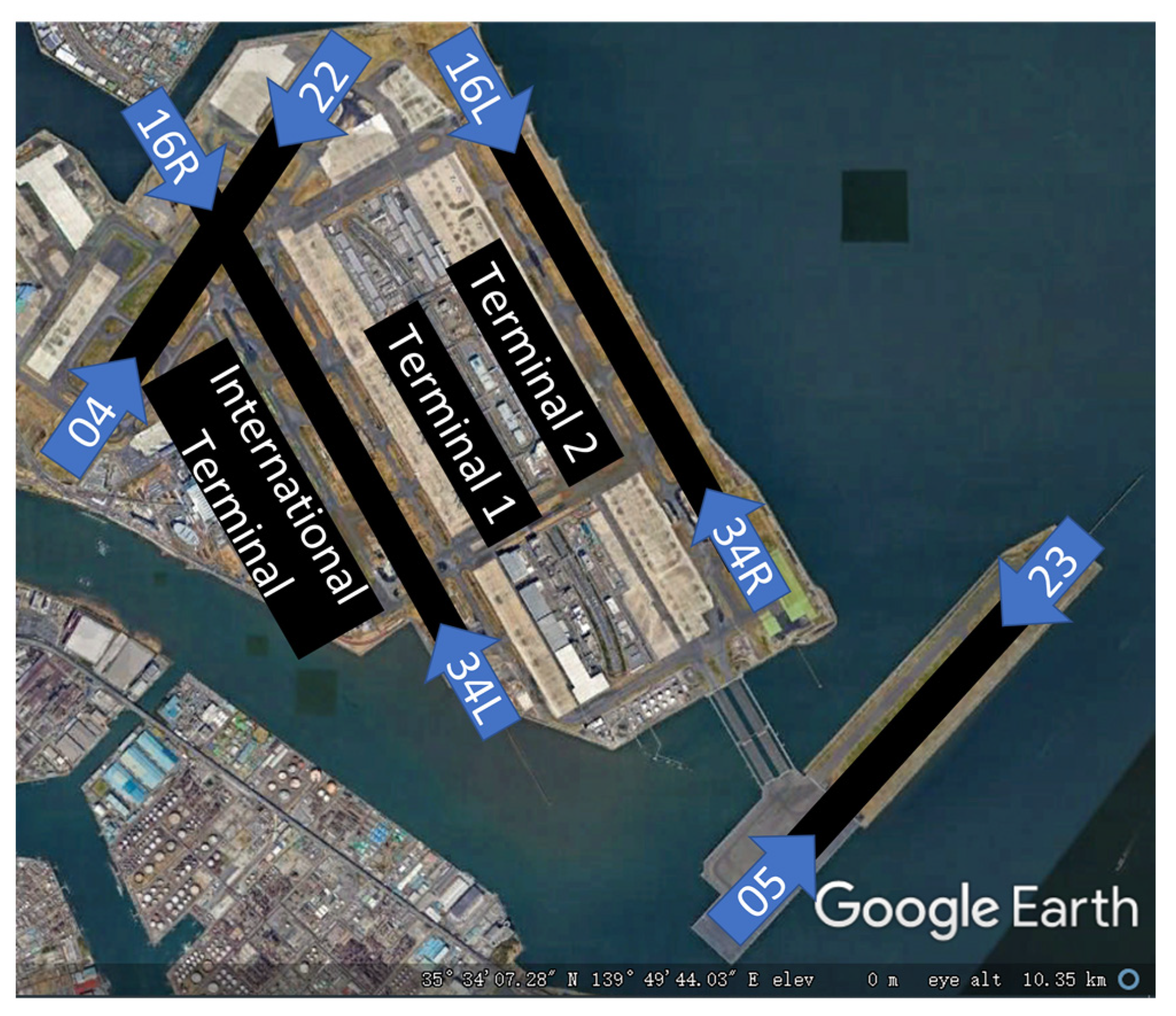
2.1. Overview of the Tokyo International Airport

Figure 1 shows the runway and terminal map of the Tokyo International Airport. It comprises four runways—16L-34R, 16R-34L, 04-22, and 05-23—which are used for take-off or landing depending on the wind direction. Basically, landing aircraft use runways 22 and 23, while take-off aircraft use runways 16L and 16R during south wind operation. However, under certain conditions, landing aircraft may use runway 16L. During north wind operation, landing aircraft use runways 34L and 34R, while take-off aircraft use runways 05 and 34R. Under certain conditions, runways 34L and 04 can be used by take-off aircraft during north wind operation.

The Tokyo International Airport has three passenger terminals: Terminal 1 (used by Japan Airlines (JAL), Skymark Airlines and Star Flyer) and Terminal 2 (used by All Nippon Airways (ANA), Air Do and Solaseed Air), which serve domestic flights; and the International Terminal (renamed as Terminal 3 on 14 March 2020), which serves international flights.

The rules of runway and terminal operation in the Tokyo International Airport were in effect in the period before 2020, which is considered in this study. To simplify the model development and implementation, south wind operation is selected in the analysis because runway 04-22 was not used during north wind operation. Late night and early morning hours are not considered since it has a different rule of runway operation under the non-congested circumstance.

2.2. CARATS Open Data

The Collaborative Actions for Renovation of Air Traffic Systems [16] is provided by the Ministry of Land, Infrastructure, Transport and Tourism in Japan as CARATS Open Data, which is in CSV format and includes the GPS ground tracking data (in seconds) of aircraft moving on the surface of Tokyo International Airport. Every second data contain the timestamp, flight ID, latitude, longitude, altitude, and aircraft type. The following information can be extracted from the CARATS Open Data for each aircraft: the flight ID, start time, end time, take-off or landing, runway ID, gate ID, and taxiway route. This information plays two roles in this study. First, it is used to identify the current surface operation pattern in this section. It is also used to evaluate and analyze the results of our optimization model in Section 4.

The flight ID, start time, and end time can be directly obtained from the CARATS Open Data. Regarding the taxiway route, every taxiway used by an aircraft needs to be identified. Four points are used to determine one taxiway or runway. These four points should form a convex polygon, and if the GPS tracking point of an aircraft enters this convex polygon, it is considered that the aircraft has passed through this taxiway or runway. One point is used to determine each gate. Using this point as the center, a circle is created for each gate with a radius of 15 m. If an aircraft appears in the circle for more than 20 s, the gate corresponding to this circle can be considered as the gate of the aircraft. The judgment of the aircraft take-off or landing is determined based on the speed. If the speed in the first 5 s of the tracking data of an aircraft exceeds 70 knots, the aircraft is considered as a landing aircraft. Otherwise, it is considered as a take-off aircraft.

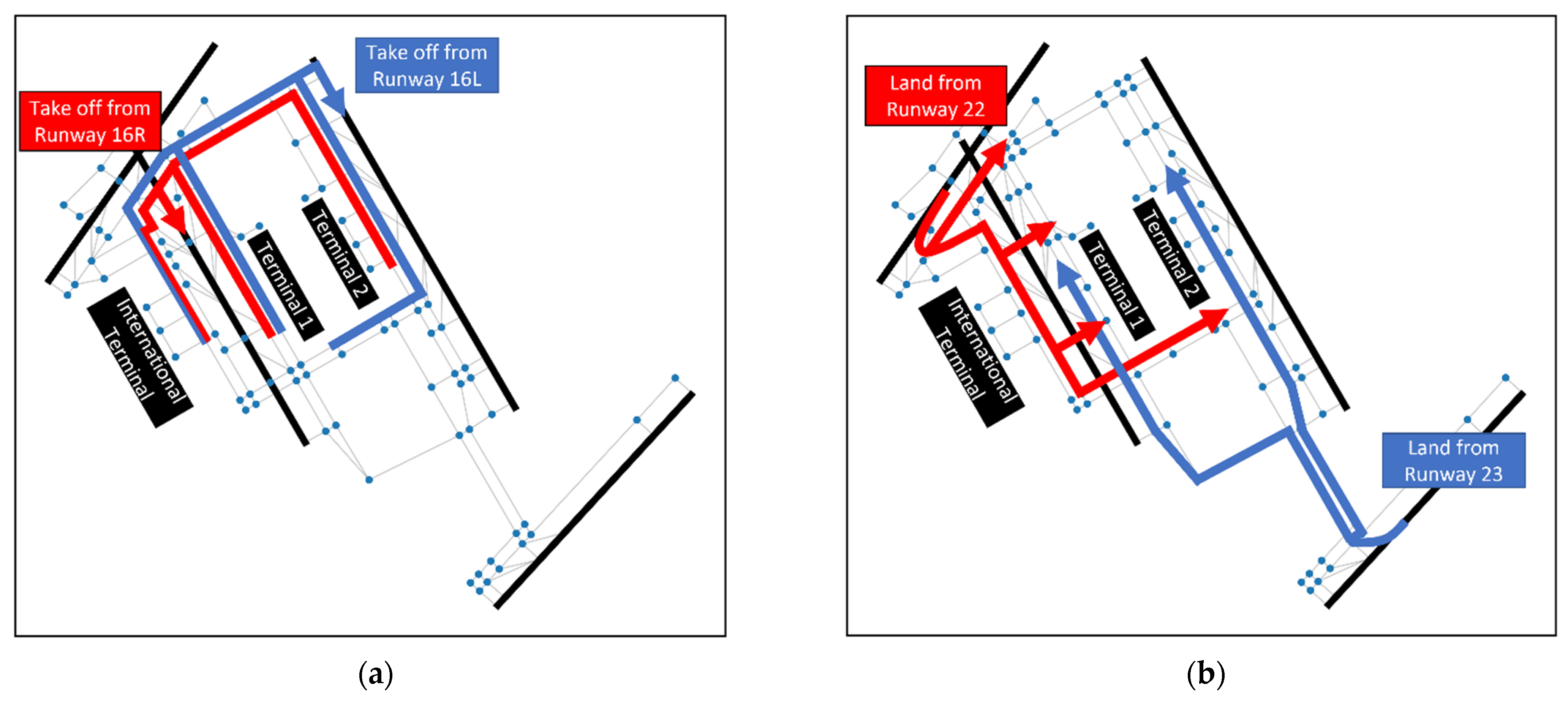
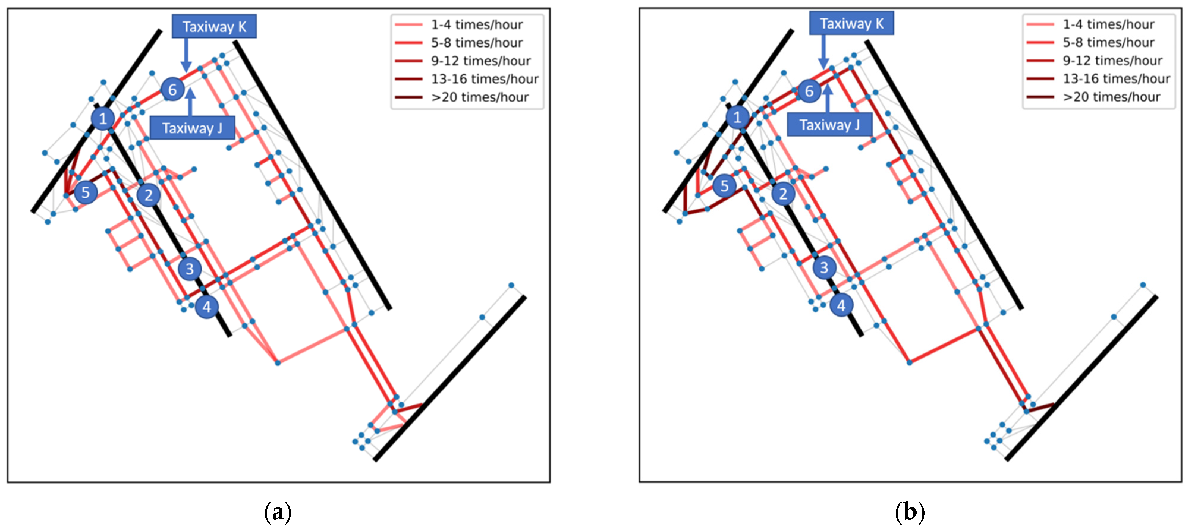
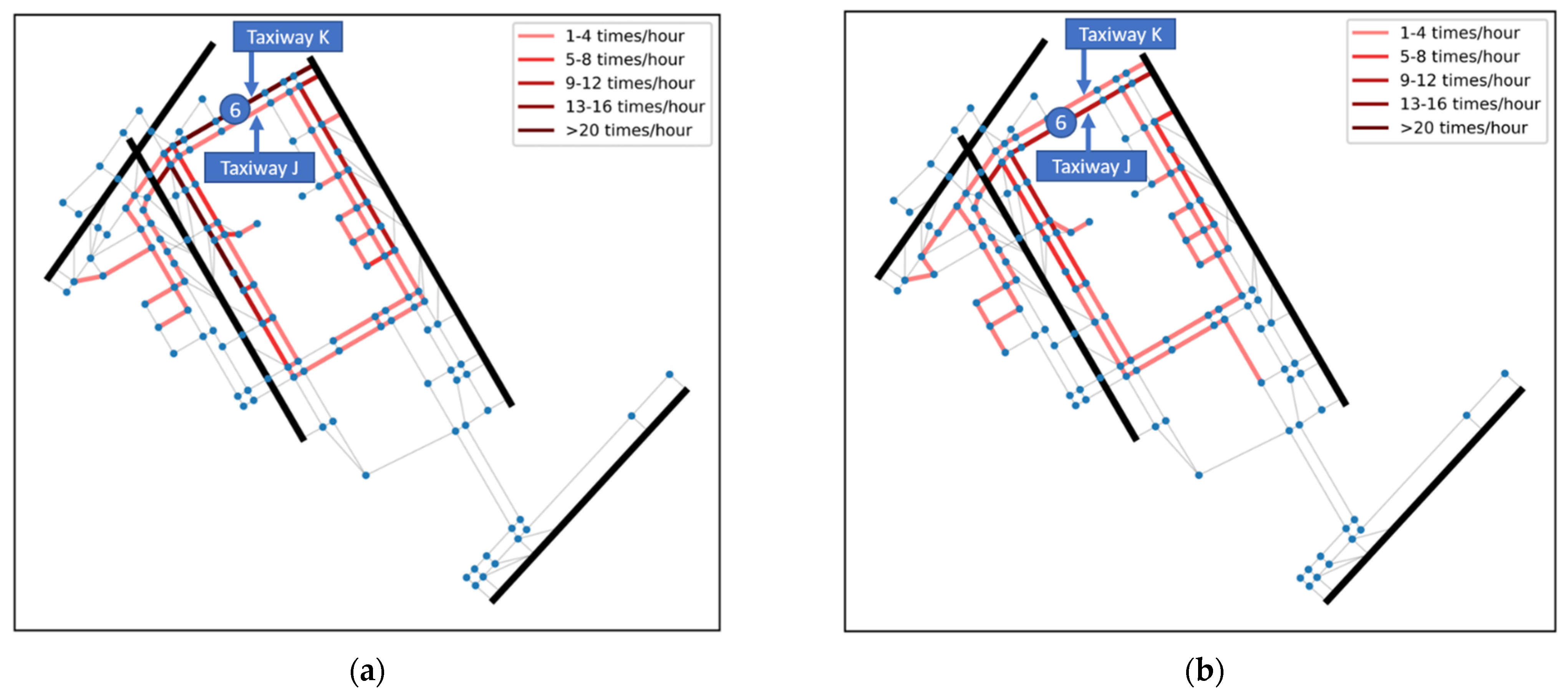
2.3. Taxiway Selection Patterns

Figure 2 shows the regular taxiway selection patterns in the observed data obtained from Tokyo International Airport. Patterns of taxiway selection indicate the most used taxiway routes, from the gate to the runway and vice versa, selected by air traffic control. The taxiway route of each aircraft is extracted from the CARATS Open Data, from which the taxiway selection pattern is obtained by finding the common sub-taxiway route of all aircraft taxiway routes. It is observed that there is usually a pattern when aircraft moves from different terminals to different runways during operation. When there are two parallel taxiways in some areas, they are used differently based on the taxi direction or destination. Considering the take-off flight in Figure 2a as an example, when an aircraft from Terminal 1 is required to take off from runway 16R, it is likely to use the red taxiway route in the figure. When it is required to take off from runway 16L, it always uses the blue taxiway route.

3. Model Development

This section describes a dynamic optimization model that is used for airport surface operations. The model dynamically outputs the ground movement route and schedule for each aircraft based on real-time flight information. Additionally, it can provide a runway choice using the runway decider module. The model aims to reduce the total ground movement distance and time of all aircraft. All mathematical notations are explained in

Table 1. Definition of mathematical notation in Section 3.

Symbol	Description
N	Set of nodes in graph model.
$N_t$	Set of taxiway intersection nodes in graph model.
$N_{entrance}$	Set of runway entrance nodes in graph model.
$N_{exit}$	Set of runway exit nodes in graph model.
$N_g$	Set of gate nodes in graph model.
$N_p$	Set of virtual push-back nodes in graph model.
$C$	Set of runway cross nodes in graph model.
$E$	Set of directed edges in graph model.
$G\left(N,E\right)$	Graph model of Tokyo International Airport.
$n_1,n_2,r_1,r_2,c,c_{t1},c_{t2},c_{r1},c_{r2}$	Identified nodes in graph model.
$L_{SP}\left(n_1,n_2\right)$	Length of shortest path between $n_1$ and $n_2$.
$g\left(n_1,n_2\right)$	Graph matrix of graph model.
$v\_max\left(n_1,n_2\right)$	Maximum taxi speed of taxiway between $n_1$ and $n_2$.
$t_{separation\_node}\left(n\right)$	Time separation requirement at node $n$.
$t_{separation\_cross}$	Time separation requirement of runway cross node.
$t_{separatio{n}_{takeoff}}\left(typ{e}_1,typ{e}_2\right)$	Time separation requirement for aircraft type $typ{e}_1$ when taking off on same runway after aircraft type $typ{e}_2$.
$F$	Set of all aircraft.
$A$	Set of all active aircraft in current planning horizon.
$a$	Identity of aircraft.
$gate\left(a\right)$	Gate node of aircraft $a$.
$start\_time\left(a\right)$	Push-back ready time for a take-off aircraft; runway arrival time for a landing aircraft.
$rwy\left(a\right)$	Runway node of aircraft $a$.
$type\left(a\right)$	Aircraft type of aircraft $a$.
$destination\left(a\right)$	Destination node of aircraft $a$.
$t_{start}\left(a\right)$	Start time of aircraft $a$ in current planning horizon.
$n_{last}\left(a\right)$	Last node passed by aircraft $a$ before current planning horizon.
$n_{start}\left(a\right)$	Node ahead of aircraft $a$ in current planning horizon.
$L_{rest}\left(a\right)$	Rest distance of aircraft $a$ to $n_{start}\left(a\right)$ in current planning horizon.
$K$	Number of steps that can be planned in one horizon.
$T$	Duration of the planning horizon.
$k,k_1,k_2$	Step number.
$x\left(a, k,n_1,n_2\right)$	Decision Variable. $x$ = 1 means aircraft $a$ taxis from $n_1$ to $n_2$ at $k^{th}$ step.
$t\left(a,k\right)$	Decision Variable. The time when aircraft a passing $k^{th}$ step’s node $n_1$.
$T_{SP}\left(n_1,n_2\right)$	The estimated taxi time from $n_1$ to $n_2$.
$t_{last}\left(n_1\right)$	Time when aircraft last passed node $n_1$ in the previous planning horizon.
$gap\left(a_1,a_2,k_1,k_2\right)$	Time gap between aircraft $a_1$ at step $k_1$ and $a_2$ at step $k_2$.
$conflict\left(a_1,a_2,k_1,k_2,n\right)$	Equals 1 when step $k_1$ of aircraft $a_1$ and step $k_2$ of aircraft $a_2$ use the same node, $n$.
$first\left(a_1,a_2,k_1,k_2\right)$	Equals 1 when the $k_1$ step of aircraft $a_1$ is performed earlier than the $k_2$ step of aircraft $a_2$.
$cross\left(a_1,a_2,k_1,k_2,c\right)$	Equals 1 if aircraft $a_1$ crosses the runway cross point $c$ at step $k_1$ when aircraft $a_2$ takes off or lands on the same runway at step $k_2$.
$firs{t}_{takeoff}\left(a_1,a_2\right)$	Equals 1 when $a_1$ takes off before $a_2$.

.

3.1. Mixed-Integer Linear Programming and Receding Horizon

This study adopts the mixed-integer linear programming (MILP) optimization, which is applicable to hybrid problems. However, the typical MILP method faces two main drawbacks in the optimization of the current research problem. First, the optimization of the airport surface operation is a type of dynamic traffic assignment problem, in which multiple coupled non-convex decisions of routing and timing are simultaneously optimized; this can be considered as an NP-hard problem. Applying a global MILP solver to handle all aircraft in one day or one hour can considerably increase the time complexity, which decelerates the solving process and inhibits the application of the approach to practical operation. Second, the optimization of airport surface operations is a dynamic problem. The prediction of when the aircraft start and arrive may be inaccurate, the predicted positions for the current aircraft may be wrong, or the predictions of when new aircraft are ready to push back from the gates or land may be wrong. Furthermore, there is a possibility that an aircraft cannot arrive, push back, or taxi as planned if the plan is determined too early, and unexpected events may occur, which can result in unsuitability of the previous plan and replanning.

A receding horizon (RH) approach, which has been extensively used in trajectory planning, is implemented to solve the above problems by dividing the MILP into several planning horizons that are sequentially optimized in the MILP solver [18,19]. A basic RH framework was first presented by Schouwenaars et al. [19]; it has been applied to the airport surface operation problem in some studies [8,13] and is adopted as the strategy of MILP optimization herein.

MILP with RH performs better for the aforementioned problem compared with the traditional MILP approach. In this approach, the global result is not obtained through a single MILP optimization. Contrarily, the planning process is divided into several horizons, similar to an iteration loop. Applying RH in MILP ensures that the computation is spread over time because of the nonlinear increase in the solving time with the problem size. On the other hand, the optimization approach could consider dynamic characteristics of airport operations, thus ensuring that the computation is not wasted on detailed plans for the distant future, which may be revised before the aircraft arrives at its destination.

The model plans for up to $K$ future steps for each aircraft at each planning horizon. After a planning horizon, the aircraft movement is simulated based on the previously established plan. The final position and status of each aircraft are considered as the input of the next planning horizon. The duration of the planning horizon follows an already set horizon time length, $T$ (s). The MILP process is as follows: plan $K$ steps, simulate and calculate for $T$ seconds, then plan the next $K$ steps based on the last results, and simulate $T$ seconds, until every aircraft arrives at its destination.

3.2. Model Parameters

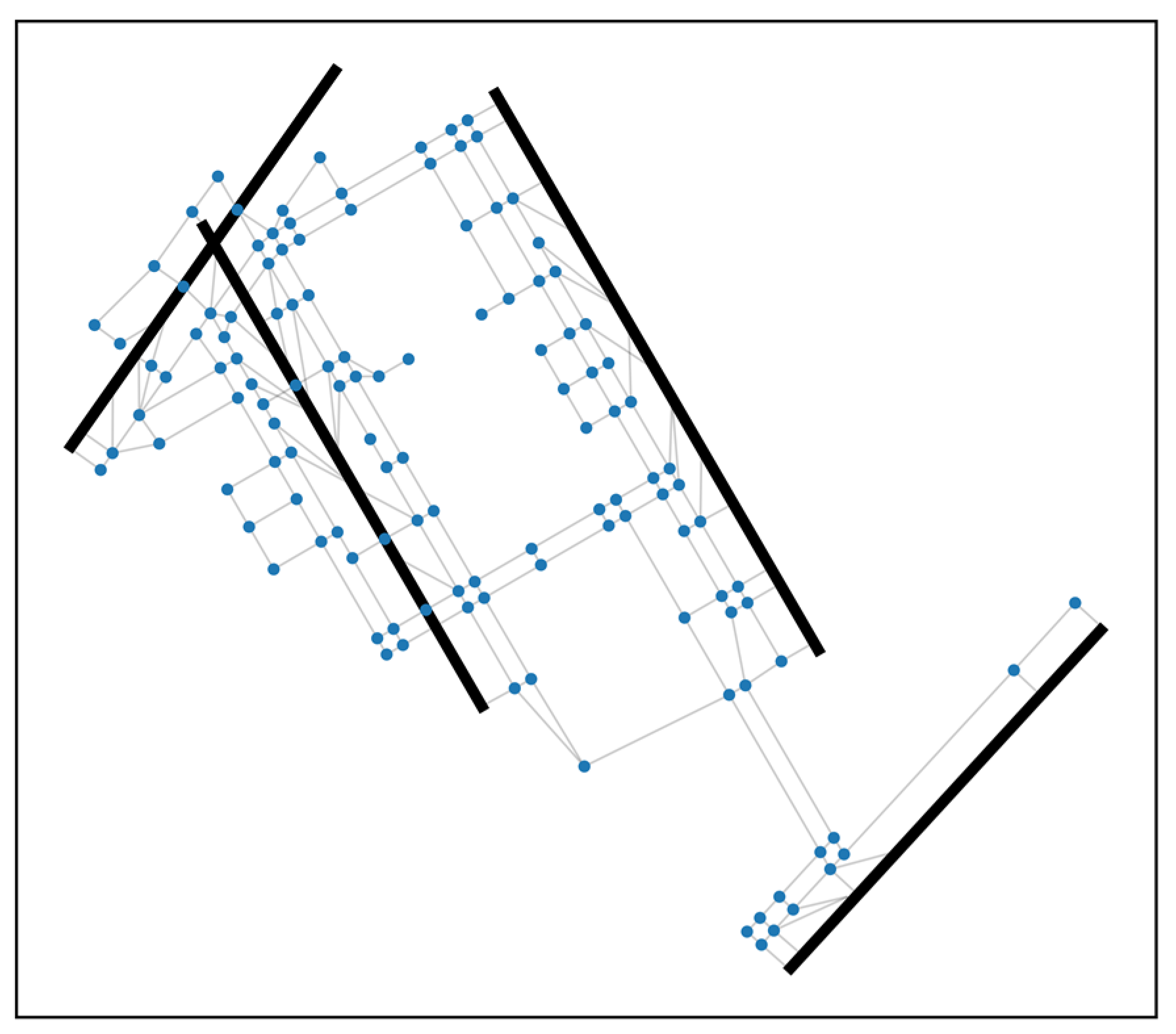
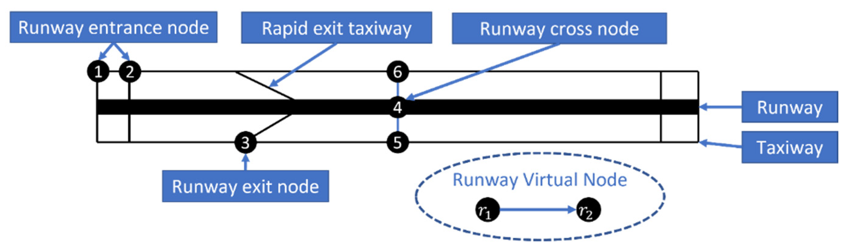
3.2.1. Airport Graph Model

A graph, $G\left(N,E\right)$, of the Tokyo International Airport was constructed to help in the development of the MILP optimization model. $N$ represents the node set, and $E$ represents the directed edge set of the graph.

$$N=\{n | n\in N_t or n\in N_{entrance} or n\in N_{exit} or n\in N_g\}$$

(1)

$\forall n_1,n_2\in N,$ if there is a taxiway can be used from $n_1{ \mathrm{to} n}_2$:

$$\left(n_1,n_2\right)\in E$$

(2)

All the taxiway intersections $N_t$, runway entrances $N_{entrance}$, runway exits $N_{exit}$, and gates $N_g$ are considered as nodes. The pairs $\left(n_1,n_2\right)$ in the set, $N$, are considered as directed edges in $E$ if there is a taxiway connection from $n_1$ to $n_2$. An overview of the graph model (excluding the gate nodes) developed after these steps is shown in Figure 3.

An adjacency matrix, $g$, is built to construct the model. $g$ is an $\left|N\right|\times \left|N\right|$ 0-1 matrix in which $g\left(n_1,n_2\right)=1$ if and only if $\left(n_1,n_2\right)\in E$. A shortest-path matrix, $L_{SP}$, is built to record the shortest distance between nodes, which is an $\left|N\right|\times \left|N\right|$ matrix calculated using the Floyd algorithm [20] shown in Algorithm 1:

Algorithm1 Floyd (G(N,E)).

let s be a |N| × |N| array initialized to ∞ (infinity)

foreach edge(u,v) in E do

s[u][v] ← l(u,v)            //l(u,v)  is the length of the edge (u,v)

foreach v in N do

s[u][v] ← 0

for k from 1 for k from 1 to |N|

for i from 1 to |N|

for j from 1 to |N|

if s[i][j] > s[i][k] + s[k][j]

s[i][j] ← s[i][k] + s[k][j]

end if

return s

Additionally, for each edge $\left(n_1,n_2\right)$, a parameter $v\_max\left(n_1,n_2\right)$ is added to represent the maximum taxi speed on that taxiway, which is decided according to the comments of operational experts from Japan Airlines. A speed of 10.29 m/s (20 knots) is set for a regular taxiway, 5.14 m/s (10 knots) is set for the taxiway near the apron area, and 25.72 m/s (50 knots) is set for the rapid-exit taxiway. For each node, $n$, $t_{separation\_node}\left(n\right)$ is set to 20 s to represent the time separation requirement at each node (see Section 3.5.2), and $t_{separation\_cross}\left(n\right)$ is set to 20 s to represent the time separation requirement for the second type of runway conflict (see Section 3.5.3).

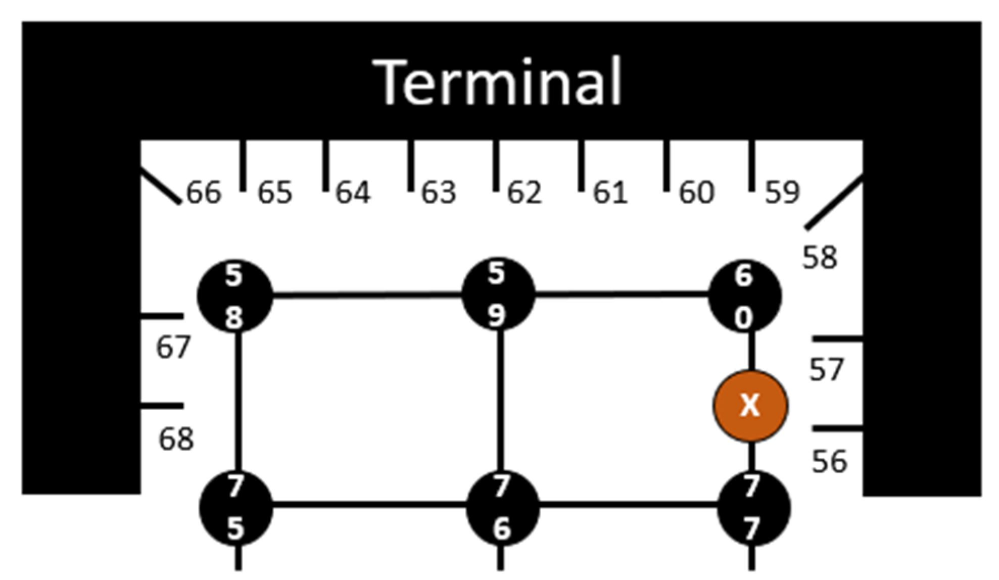
3.2.2. Virtual Pushback Node

A virtual pushback node system is developed for the aircraft to find its start or end nodes in the optimization model. In a few previous studies, the departure aircraft of a specific terminal usually starts at the same node in the graph model. The scale of the model can be reduced by using these merged nodes. However, the taxiway usage in the area near the gate and the specific situation when multiple aircraft are pushed back cannot be simulated. In order to overcome these drawbacks, this study proposes a pushback node system as the terminal and apron areas of the Tokyo International Airport are closely related to the taxi area. A new virtual pushback node is inserted in the middle of each taxiway that is near the terminal area and is connected to the gates. It divides the original taxiway into two sub-taxiways. This node is assigned as the pushback point to the gates connected to the specific taxiway. The departure and arrival aircraft using these gates consider these pushback nodes as their origins and destinations, respectively. Using Figure 4 as an example, a new node X is added between node 60 and node 77, which divides edge (60, 77) into two edges: (60, X) and (X, 77). Node X is set as the pushback node for nearby gates 56 and 57. All the virtual pushback nodes, $N_p$, are also considered as nodes in $N$. Concurrently, the edge set, $E$, is adjusted accordingly depending on the insertion of these nodes and the division of the edges.

3.2.3. Runway Virtual Node and Cross Node

As the take-off, landing, and sequencing processes are considered in the model, a corresponding node system is designed in the graph model. Two virtual nodes, $r_1$ and $r_2$, are added for each runway, and they are connected by a virtual directed edge ( $r_1$, $r_2$ ).

Assuming Figure 5 represents a take-off runway, virtual edges (1, $r_1$ ) and (2, $r_1$ ) are added to connect the runway entrance node to the runway virtual node. Aircraft enter the runway through the runway entrance node and line up at node $r_1$; they take-off at the edge ( $r_1$, $r_2$ ) and arrive at their destinations at node $r_2$ in the optimization model. Assuming Figure 5 represents a landing runway, virtual edge ( $r_2$, 3) is added to connect the runway virtual node to the runway exit node. Landing aircraft start at node $r_1$ in the optimization model, land on edge ( $r_1$, $r_2$ ), exit the runway at node $r_2$, and taxi to runway exit node 3.

In the Tokyo International Airport, there are runway cross points on runway 16R-34L and runway 04-22, where aircraft can taxi across the runway. To design the constraints to avoid cross conflict in Section 3.5.3, a runway cross node system as that shown in Figure 5 is designed. For each cross node $c$ (node 4 in Figure 5) in runway cross node set $C$, $c_{r1}, c_{r2}$ (node $r_1$ and node $r_2$ in Figure 5) represent the two runway virtual nodes used for take-off or landing on the runway, while $c_{t1},c_{t2}$ (node 5 and node 6 in Figure 5) represent the two nodes of the taxiway that cross the runway.

All the runway virtual nodes and cross nodes are considered as nodes in $N$. Concurrently, the edge set, $E$, is adjusted accordingly depending on the insertion of these nodes and edges.

3.2.4. Aircraft Data

For the entire optimization model, set $F$ includes all the aircraft considered in the optimization. Each aircraft $a$ in $F$ has some static parameters given as follows: $gate\left(a\right)$ represents the gate node of aircraft $a$; $start\_time\left(a\right)$ represents the pushback ready time of a departure aircraft and the time of arrival at the runway of an arrival aircraft; $rwy\left(a\right)$ represents the runway of aircraft $a$; $type\left(a\right)$ represents the aircraft type of aircraft $a$; and $destination\left(a\right)$ represents the destination node of aircraft $a$ in the optimization model. For a take-off aircraft, $destination\left(a\right)$ is the runway virtual node $r_2$ of $rwy\left(a\right)$ (see Section 3.2.3), and for a landing aircraft, $destination\left(a\right)$ is the corresponding virtual pushback node of $gate\left(a\right)$ (see Section 3.2.2).

In a specific planning horizon, the active aircraft set $A$ includes the aircraft that has a start time later than the time of the current horizon and has not reached its destination. For each aircraft $a$ in $A$, $t_{start}\left(a\right), n_{last}\left(a\right),n_{start}\left(a\right)$, and $L_{rest}\left(a\right)$ are used to define the start time and position in the current planning horizon. At time $t_{start}\left(a\right)$, aircraft $a$ taxis from $n_{last}\left(a\right)$ to $n_{start}\left(a\right)$, at a distance, $L_{rest}\left(a\right)$ away from $n_{start}\left(a\right)$. For a newly added aircraft to the planning horizon, $n_{last}\left(a\right)$ is the gate node $gate\left(a\right)$, $n_{start}\left(a\right)$ is the corresponding pushback node, $L_{rest}\left(a\right)$ is equal to $L_{SP}\left(n_{last}\left(a\right),n_{start}\left(a\right)\right)$ , and $t_{start}\left(a\right)$ equals to $start\_time\left(a\right)$. If an aircraft has already been added in the previous planning horizons, $n_{last}\left(a\right),n_{start}\left(a\right)$, and $L_{rest}\left(a\right)$ are calculated from the result of the last horizon, and $t_{start}\left(a\right)$ is equal to the start time of the current planning horizon.

3.3. Decision Variables

In an MILP planning horizon, each aircraft performs K step movements, which means taxiing through K edges in the graph, $G\left(N,E\right)$. As the model determines the taxi route and schedule of the aircraft, the information of each movement includes the target node and time of arrival at the node of each step. Clare, Richards and Sharma [21] proposed to include the above information into MILP by implementing two decision variables. Variable $x$ represents the taxi route, which is applied as a binary variable $x\left(a, k,n_1, n_2\right)$ to MILP, in which $a\in A, 1\le k\le K, n_1,n_2\in N$. $x\left(a, k,n_1, n_2\right)$ equals 1, which means that aircraft $a$ taxis from start node $n_1$ to target node $n_2$ at the $k$ th step in the plan. Another non-negative integer variable, $t\left(a,k\right)$, determines the taxi schedule, where $a\in A, 1\le k\le K+1$. $t\left(a,k\right)$ represents the time when $a$ passes the start node, $n_1$, of its $k$ th step. Particularly, $t\left(a,1\right)$ is the start time of $a$ when it is at the start location of the current planning horizon, and $t\left(a,K+1\right)$ is the time when $a$ passes the target node $n_2$ of its final step.

3.4. Objective Function

Two parts are considered in the final objective function to define an objective for each MILP planning horizon. First, the total taxi distance of all the aircraft in the current horizon are minimized. In conventional global optimization, the total taxi distance of all the aircraft is directly set in one day or in several hours. However, in the model, the aircraft cannot arrive at their destinations in one horizon, and the regular objective function, which is given in Equation (3), cannot include the remaining taxi distances in the future; thus, the MILP model loses its direction.

$${\displaystyle \sum }_{a\in A}\left({\displaystyle \sum }_a^A{\displaystyle \sum }_{n_1}^N{\displaystyle \sum }_{n_2}^N{\displaystyle \sum }_k^K{L}_{SP}\left(n,m\right)\ast x\left(a, k,n_1,n_2\right)\right)$$

(3)

This is a common problem when applying RH into MILP optimization. The design of the objective function in this study is based on the cost-to-go function computed by using the shortest-path algorithm [22]. In addition, Clare, Richards and Sharma [21] applied this approach to solve the airport ground movement optimization problem. Our model uses the real taxi distance that is already planned in the current horizon plus an estimated taxi length from the current position to the destination using the shortest-path length.

In Equation (4), $ob{j}_{distance}$ is an alternative total taxi distance. The first term of Equation (4) represents the total taxi distance in the current planning horizon. The second term of Equation (4) represents the estimated taxi distance of $a$ from the current planning horizon until its destination using the shortest-path length.

$$\begin{array}{cc}\hfill ob{j}_{distance}=& {\displaystyle \sum _{a\in A}}({\displaystyle \sum _{n_1\in N}}{\displaystyle \sum _{n_2\in N}}{\displaystyle \sum _{k=1}^K}{L}_{SP}\left(n_1,n_2\right)\ast x\left(a, k,n_1,n_2\right)\hfill \\ & +{\displaystyle \sum _{n_1\in N}}{\displaystyle \sum _{n_2\in N}}{L}_{SP}\left(n_2,destination\left(a\right)\right)\ast x\left(a, K,n_1,n_2\right))\hfill \end{array}$$

(4)

$$T_{SP}\left(n_1,n_2\right)=\{\begin{array}{c}\frac{L_{SP}\left(n_1,n_2\right)}{v\_max\left(n_1,n_2\right)}+120, n_2 is runway virtual node but n_1 is not\hfill \\ \frac{L_{SP}\left(n_1,n_2\right)}{v\_max\left(n_1,n_2\right)}, otherwise\hfill \end{array}$$

(5)

$$ob{j}_{time}={\displaystyle \sum }_{a\in A}\left(t\left(a,K+1\right)-t_{start}\left(a\right)+{\displaystyle \sum }_{n_1\in N}{\displaystyle \sum }_{n_2\in N}x\left(a, K,n_1,n_2\right)\times T_{SP}\left(n_2,destination\left(a\right)\right)\right)$$

(6)

$$\left(\mathrm{Minimize}\right) obj=ob{j}_{distance}{}_{ }+w\ast ob{j}_{time}$$

(7)

In addition to the total taxi distance, the taxi time must also be considered, thus avoiding wasting time during taxiing. In Equation (6), $ob{j}_{time}$ is an alternative total taxi time using the same estimated method as for $ob{j}_{distance}$. The first term of Equation (6) represents the total taxi time length of aircraft $a$ in the current planning horizon. The second term of Equation (6) indicates the estimated taxi time length of $a$ from the current planning horizon until its destination. The estimated taxi time length is calculated from Equation (5). Basically, the estimated taxi time is calculated as the shortest-path length divided by the maximum speed. However, to improve the performance when a take-off aircraft does not reach the runway virtual node and ready-for-take-off point in the current planning horizon (see Section 4.5), an additional virtual long waiting time (120 s) is added to $ob{j}_{time}$. This is considered as part of the estimated taxi time length from the current planning horizon to the destination. The addition of this part can help the MILP model face congestion on the runway directly, without making meaningless detours.

The final objective function in Equation (7) is a weighted combination of $ob{j}_{distance}$ and $ob{j}_{time}$, which need to be minimized. A non-negative weight parameter, $w$ is used in ${\mathit{obj}}_{\mathit{time}}$ to control the weights of two sub-objective functions. From the equation, it can be inferred that small $w$ values can produce better optimization of the global taxi distance, whereas large $w$ values can reduce waiting times for the aircraft. The effect of this weight, owing to the application of RH, on the results is discussed comprehensively in Section 4.4. Herein, $w$ = 1.5.

3.5. Constraints

3.5.1. Constraints for Taxi Rules on the Graph Model

The taxiway and airport rules are added to the constraints. It should be noted that Equations (8)–(10), (12), and (14) refer to the model proposed in the same study [21] as the one used to determine the decision variables in Section 3.3. Equations (8) and (9) ensure that each aircraft only taxis on one existing edge at each step. Equation (10) ensures that the aircraft starts from the node where it arrived at the previous step. Equation (11) ensures that the aircraft does not use the edge of the previous step in the opposite direction.

$${\displaystyle \sum }_{n_1\in N}{\displaystyle \sum }_{n_2\in N}x\left(a, k,n_1, n_2\right)=1\hspace{1em}\hspace{1em}a\in A, 1\le k\le K$$

(8)

$$g\left(n_1,n_2\right)-x\left(a, k,n_1,n_2\right)\ge 0\hspace{1em}\hspace{1em}{n}_1,n_2\in N, a\in A, 1\le k\le K$$

(9)

$${\displaystyle \sum }_{n_2\in N}x\left(a, k-1, n_2,n_1\right)={\displaystyle \sum }_{n_2\in N}x\left(a, k,n_1,n_2\right)\hspace{1em}\hspace{1em}{n}_1\in N, a\in A, 2\le k\le K$$

(10)

$$x\left(a, k-1,n_1,n_2\right)+x\left(a, k,n_2,n_1\right)\le 1\hspace{1em}\hspace{1em}{n}_1,n_2\in N,a\in A, 2\le k\le K$$

(11)

Here, $n_{last}\left(a\right),n_{start}\left(a\right)$, and $L_{rest}\left(a\right)$ are used to define the start position of aircraft $a$ in each planning horizon, as discussed in Section 3.2.4. At the start time of the current planning horizon, aircraft $a$ taxis from $n_{last}\left(a\right)$ to $n_{start}\left(a\right)$, and is located at a distance $L_{rest}\left(a\right)$ from $n_{start}\left(a\right)$. $t_{start}\left(a\right)$ defines the start time of aircraft $a$ in current planning horizon. These parameters are constrained by Equations (12) and (13). An aircraft taxiing along the taxiway must follow the maximum taxi speed of the current taxiway, which is constrained by Equation (14).

$$\begin{array}{c} x\left(a, 1,n_{last}\left(a\right),n_{start}\left(a\right)\right)=1 a\in A\hfill \end{array}$$

(12)

$$\begin{array}{c}\forall a\in A: \hfill \\ t\left(a,1\right)=t_{start}\left(a\right) \hfill \\ t\left(a,2\right)\ge \frac{L_{rest}\left(a\right)}{v\_max\left(n_{last}\left(a\right),n_{start}\left(a\right)\right)}+t_{start}\left(a\right) \hfill \end{array}$$

(13)

$$\begin{array}{c}\forall a\in A, 3\le k\le K+1: \hfill \\ t\left(a,k\right)-t\left(a,k-1\right)\ge \frac{{\displaystyle {\sum }_{n_1\in N}}{\displaystyle {\sum }_{n_2\in N}}{L}_{SP}\left(n_1,n_2\right) \ast x\left(a, k-1,n_1, n_2\right)}{v\_max\left(n_1,n_2\right)}\hfill \end{array}$$

(14)

$$\begin{array}{c}\forall a_1,a_2\in A, 1\le k_1,k_2\le K+1:\hfill \\ gap\left(a_1,a_2,k_1,k_2\right)=t\left(a_1,k_1\right)-t\left(a_2,k_2\right)\hfill \\ ga{p}_{abs}\left(a_1,a_2,k_1,k_2\right)=\left|gap\left(a_1,a_2,k_1,k_2\right)\right| \hfill \end{array}$$

(15)

$$\begin{array}{c}\forall a_1,a_2\in A, 2\le k_1,k_2\le K, n_1\in N:\hfill \\ conflict\left(a_1,a_2,k_1,k_2, n_1\right)\hfill \\ =and\left({\displaystyle \sum _{n_2\in N}}x\left(a_1,k_1,n_1,n_2\right),{\displaystyle \sum _{n_2\in N}}x\left(a_2,k_2,n_1,n_2\right)\right) \hfill \end{array}$$

(16)

$$first\left(a_1,a_2,k_1,k_2\right)=0 or 1 \forall a_1,a_2\in A, a_1<a_2,1\le k_1,k_2\le K.$$

(17)

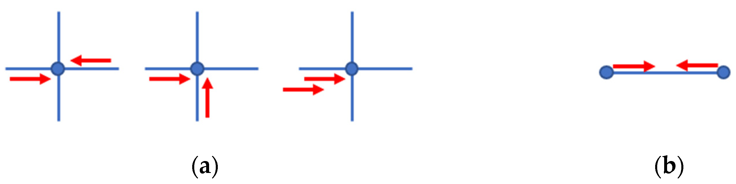
3.5.2. Constraints to Avoid Conflict on Taxiways

To define the constraints for aircraft conflict on taxiways, some temporary variables are added to the model. The temporary variables, $gap\left(a_1,a_2,k_1,k_2\right)$, are used in Equation (15) and correspond to the time gap between aircraft $a_1$ at step $k_1$ and $a_2$ at step $k_2$. In Equation (16), the binary variable, $conflict\left(a_1,a_2,k_1,k_2,n\right)$, equals 1 when step $k_1$ of aircraft $a_1$ and step $k_2$ of aircraft $a_2$ use the same node, $n$. In Equation (17), the binary variable $first\left(a_1,a_2,k_1,k_2\right)$ equals 1 when the $k_1$ step of aircraft $a_1$ is performed earlier than the $k_2$ step of aircraft $a_2$.

Figure 6 shows two types of aircraft conflict on a taxiway. The first type of conflict is a general conflict at each node. It is used as a constraint in Equation (18) as the time separation is required between each aircraft using the same node. Additionally, a second type of constraint is considered in Equations (19) and (20) to avoid head-to-head conflict between two aircraft using the same taxiway from different directions, where ‘ $\to$ ’ represents the indicator constraints that can be solved in an MILP solver such as Gurobi. An indicator constraint $z=f\to a^{T}x\le b$ states that if the binary indicator variable $z$ is equal to $f$, then the linear constraint should hold. Equation (21) is used to prevent an aircraft from conflicting with the last planning horizon aircraft, where $t_{last}\left(n_1\right)$ represents the time when the aircraft last crossed node $n_1$ in the previous planning horizon.

$$\begin{array}{c}\forall a_1,a_2\in A, 2\le k_1,k_2\le K,n\in N:\hfill \\ conflict\left(a_1,a_2,k_1,k_2,n\right)=1 \to ga{p}_{abs}\left(a_1,a_2,k_1,k_2\right)\ge t_{separation\_node}\left(n\right).\hfill \end{array}$$

(18)

$$\forall a_1,a_2\in A, a_1<a_2, 1\le k_1,k_2\le K,n\in N:$$

$$\begin{array}{c}first\left(a_1,a_2,k_1,k_2\right)=0 \to ga{p}_{abs}\left(a_1,a_2,k_1,k_2+1\right)\hfill \\ \hspace{1em}\ge t_{separation\_node}\left(n\right)-BIGM\ast \left(2-x\left(a_1,k_1,n_1,n_2\right)-x\left(a_2,k_2,n_2,n_1\right)\right)\hfill \end{array}$$

(19)

$$\begin{array}{c}first\left(a_1,a_2,k_1,k_2\right)=1 \to ga{p}_{abs}\left(a_1,a_2,k_2,k_1+1\right)\hfill \\ \hspace{1em}\ge t_{separation\_node}\left(n\right)-BIGM\ast \left(2-x\left(a_1,k_1,n_1,n_2\right)-x\left(a_2,k_2,n_2,n_1\right)\right)\hfill \end{array}$$

(20)

$$\begin{array}{c}\forall a\in A, 2\le k\le K,n_1\in N:\hfill \\ t\left(a,k\right)\ge {\displaystyle \sum _{n_2\in N}}\left(t_{last}\left(n_1\right)+t_{separatio{n}_{node}}\left(n_1\right)\right)\ast x\left(a, k,n_1, n_2\right)\hfill \end{array}$$

(21)

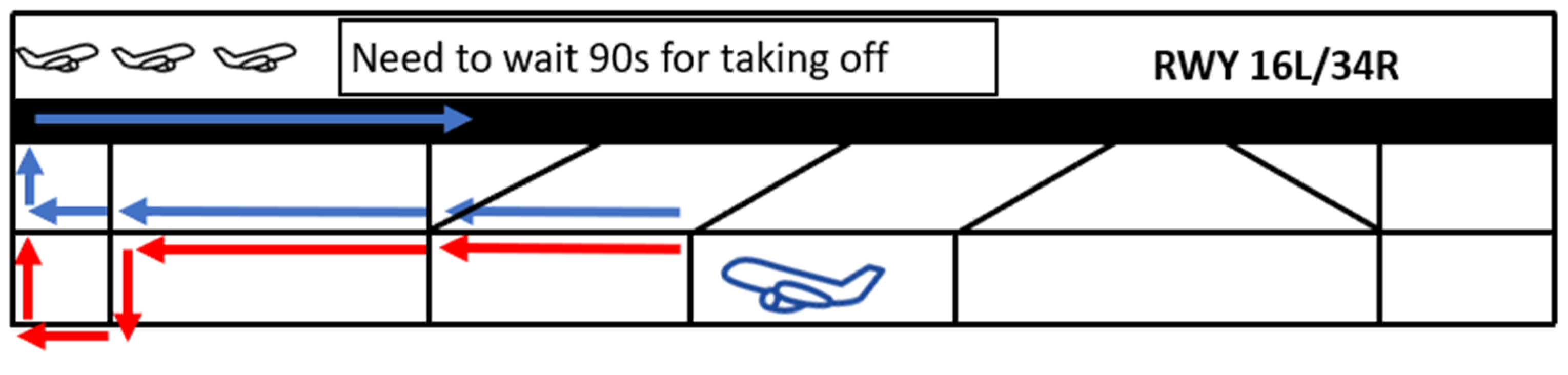
3.5.3. Constraints to Avoid Conflict in the Runway

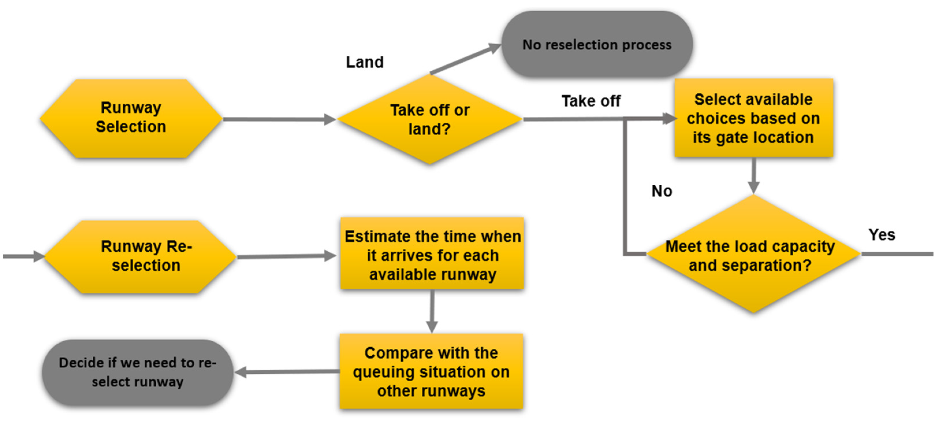
Two types of conflict on the runway are considered in this study. First, during taxiing, aircraft can cross runway 16R-34L or runway 04-22. It is necessary to prevent these aircraft from conflicting with aircraft that are currently taking off or landing on the corresponding runway.

A temporary binary variable, $cross\left(a_1,a_2,k_1,k_2,c\right)$, is shown in Equation (22). It is equal to 1 if aircraft $a_1$ crosses the runway cross point $c$ at step $k_1$ when aircraft $a_2$ takes off or lands on the same runway at step $k_2$. In Equation (23), a temporary binary variable, $firs{t}_{takeoff}\left(a_1,a_2\right)$, is used to determine the take-off order between aircraft $a_1$ and $a_2$. It is equal to 1 when $a_1$ takes off before $a_2$.

$$\begin{array}{c}\forall a_1,a_2\in A, 2\le k_1,k_2\le K, c\in C:\hfill \\ cross\left(a_1,a_2,k_1,k_2,c\right)=and\left(x\left(a_1,c_{t1},c_{t2},k_1\right),x\left(a_2,c_{r1},c_{r2},k_2\right)\right)\hfill \end{array}$$

(22)

$$\begin{array}{c}\forall a_1,a_2\in A:\hfill \\ firs{t}_{takeoff}\left(a_1,a_2\right)=0 or 1\hfill \\ firs{t}_{takeoff}\left(a_1,a_2\right)+ firs{t}_{takeoff}\left(a_2,a_1\right)=1\hfill \end{array}$$

(23)

$$\begin{array}{c}\forall a_1,a_2\in A, 2\le k_1,k_2\le K,c\in C:\hfill \\ cross\left(a_1,a_2,k_1,k_2,c\right)=1 \to ga{p}_{abs}\left(a_1,a_2,k_1,k_2\right)\ge t_{separation\_cross} \hfill \end{array}$$

(24)

$$\begin{array}{c}\forall a_1,a_2\in A, 2\le k_1,k_2\le K,r\in R:\hfill \\ and\left(conflict\left(a_1,a_2,k_1,k_2,r\right),firs{t}_{takeoff}\left(a_1,a_2\right)\right)=1\to \hfill \\ gap\left(a_2,a_1,k_2,k_1\right)\ge t_{separation\_takeoff}\left(type\left(a_1\right),type\left(a_2\right)\right)\hfill \end{array}$$

(25)

Equation (24) shows the constraint that is used to avoid the first type of conflict. If aircraft $a_1$ and $a_2$ have $cross\left(a_1,a_2,k_1,k_2,c\right)=1$ at steps $k_1$ and $k_2$ at cross point $c$, then their time gap must exceed the set separation requirement of the runway cross point.

Equation (25) is used to prevent another type of conflict in which two take-off aircraft use the same runway. These aircraft must follow a time separation requirement set by parameter $t_{separation\_takeoff}$, which is obtained from the official document “Control service processing procedure” adopted by the Tokyo International Airport. The document divides aircraft into groups A to G; different groups of aircraft have different time separation requirements when using the same runway successively, based on safety rules and on rear turbulence phenomena.

3.6. Runway Decider

Runway schedule and sequencing are determined in the MILP model based on the aforementioned constraints. However, runway management at the Tokyo International Airport also includes runway selection. According to Section 2, the airport provides two runway options for aircraft during take-off or landing. The difference in the selection can affect the taxi distance and the time to the target terminal gate. Thus, this study proposes the application of a runway decider for runway reselection. As the optimization model is developed only for airport surface operation, the landing aircraft is considered after it arrives and leaves the runway. Therefore, it is difficult to change the runway selection for the landing aircraft. For the take-off aircraft, the selection of the take-off runway is mainly based on the flight destination and its air route during actual operation. However, runway reselection is still attempted based on the runway-terminal relationship.

The runway decider is a two-stage workflow, as shown in Figure 7. The first stage is performed before the entire optimization model when the aircraft data are input. During the first stage, the best choice of runway for a take-off aircraft is selected based on its gate location. If the selection cannot meet the load capacity of the runway, the second-best choice is selected. The first stage can provide a runway selection result beforehand. During the second stage, the time when each aircraft arrives at the runway entrance is estimated, and its take-off time is calculated at both the available runways based on the queuing situation and the take-off time separation. If the other runway choice is better and its capacity is not exceeded, it is reselected in the second stage. This is a detachable module for the above optimization model, which is convenient for subsequent analysis.

4. Results and Discussion

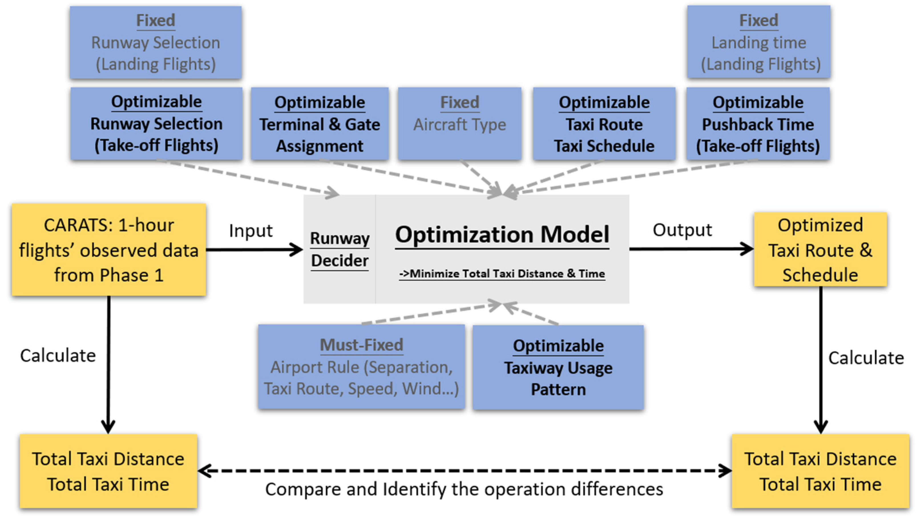
4.1. Implementation

Figure 8 shows the model implementation workflow, of which the central part is the model developed in Section 3. The CARATS Open Data are used as the model input. It contains the GPS ground tracking data of the aircraft in seconds, as obtained from the Tokyo International Airport. After the data processing detailed in Section 2, the following information is extracted for each flight: flight ID, start time, take-off or landing, runway ID, gate ID, and taxiway route. A one-hour range from 17:00 to 18:00 was selected on 9 May 2016, for this implementation. In this time range, the details of 34 take-off aircraft and 40 landing aircraft were recorded to be used as input data. For the MILP model, we assumed $K=5$ and $T=50 \mathrm{s}$.

The model was built in Python, and the MILP optimization part was built with the help of the Gurobipy Python library. Gurobi 9.11 was used as the MILP solver. The model was run on an Intel Core i5-10400 4.3 GHz PC with 16 GB RAM. An optimized result that includes the taxi route and schedule was obtained from the developed optimization model.

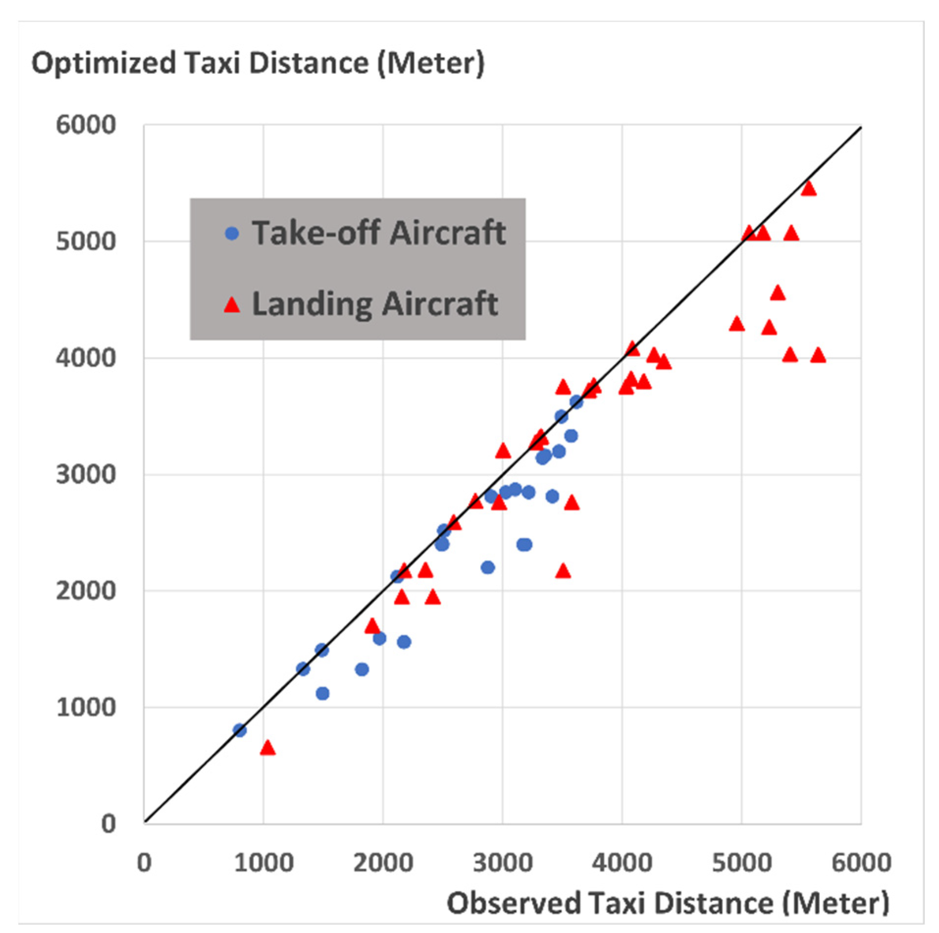
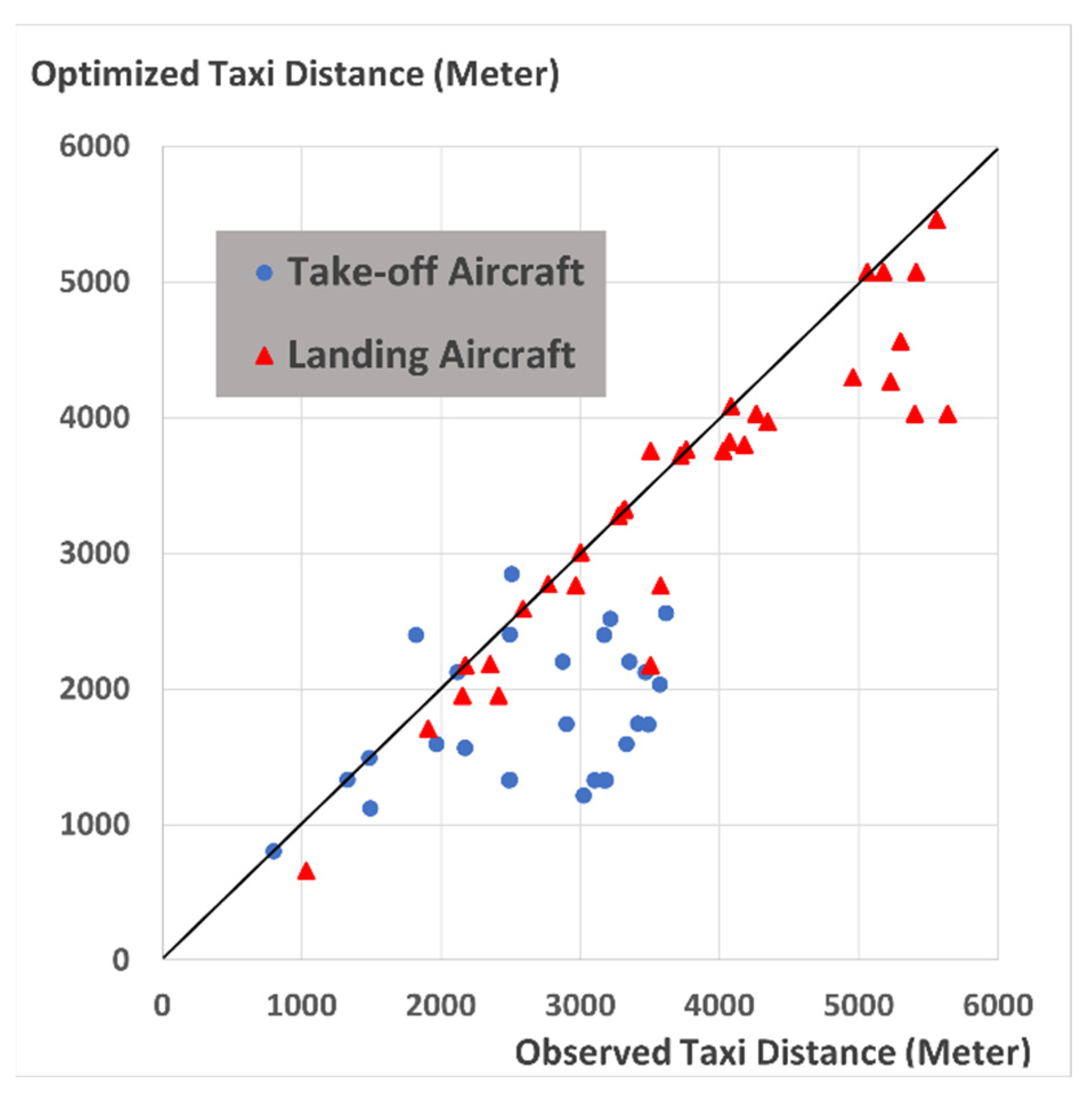
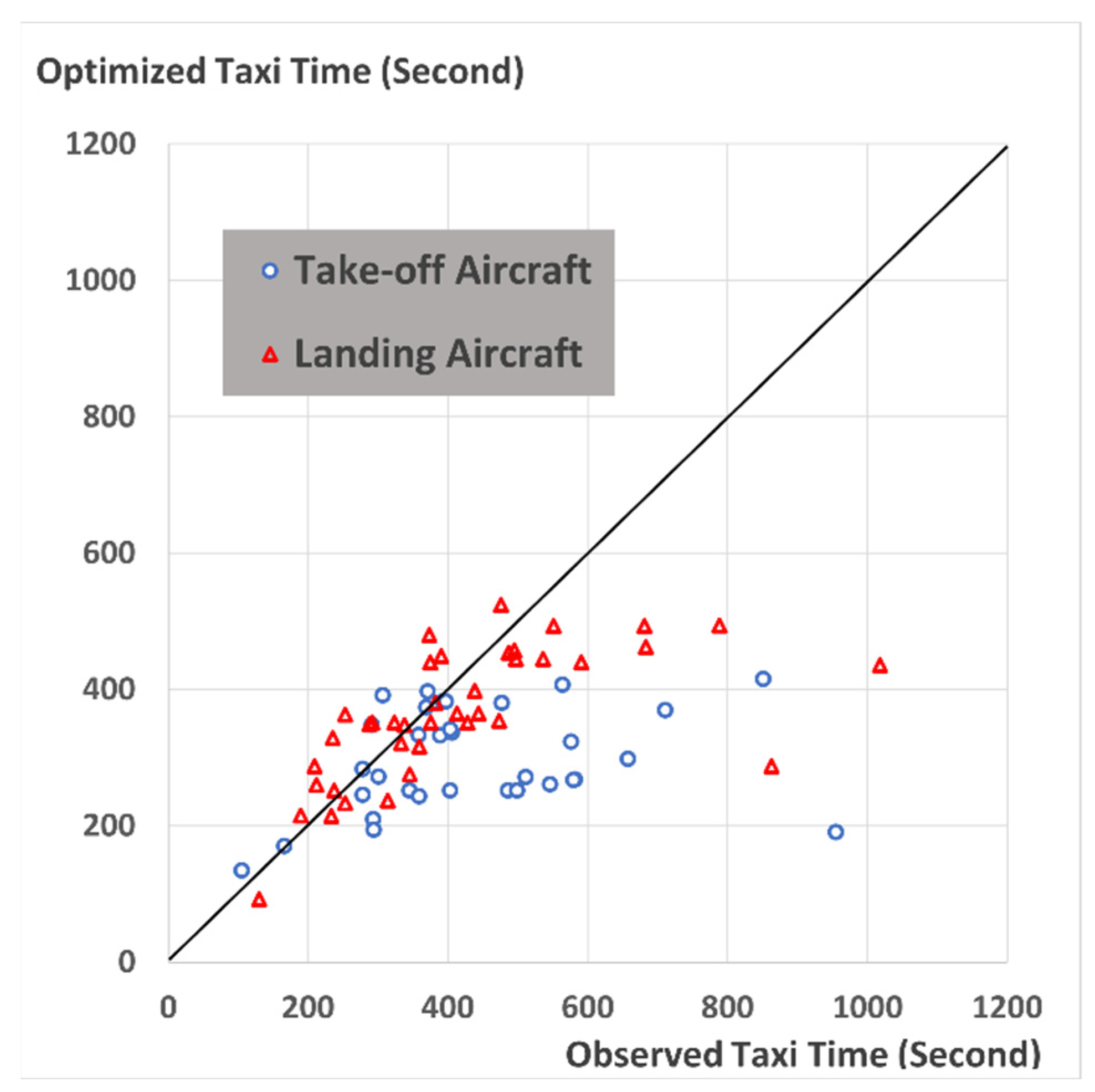
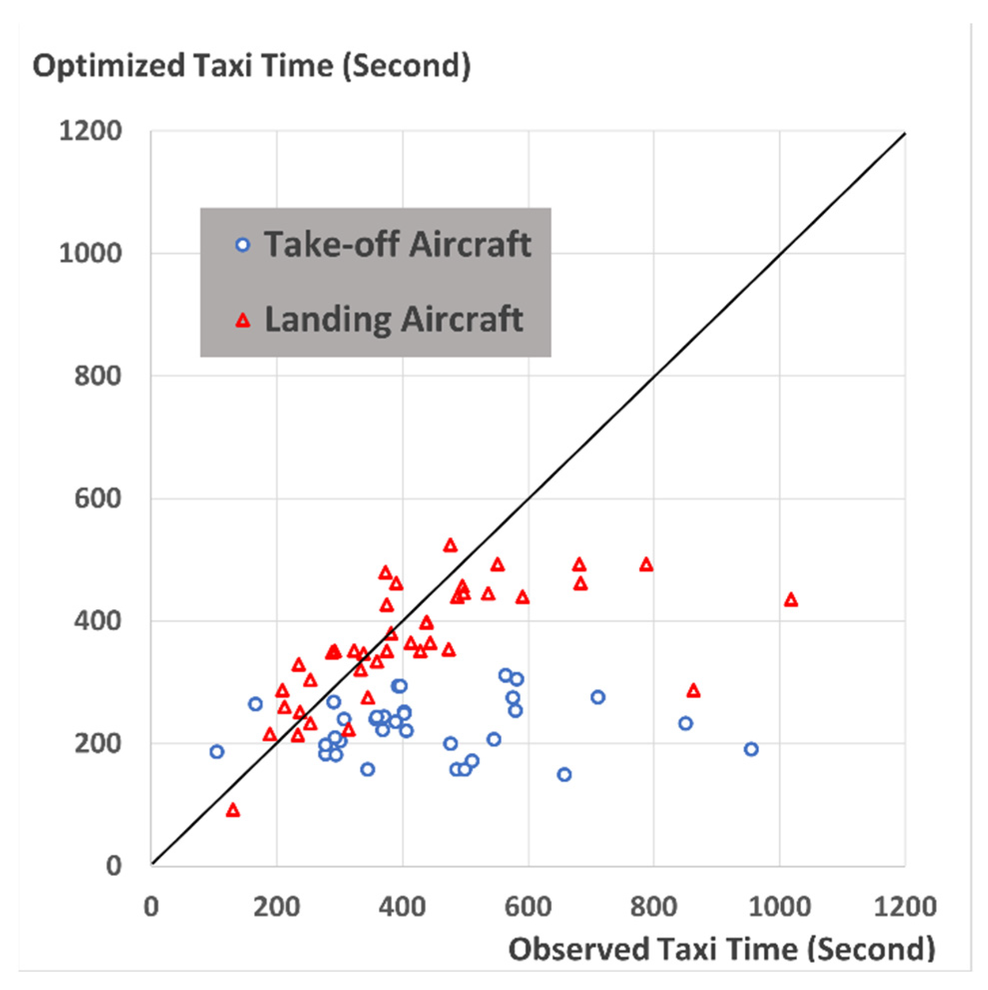
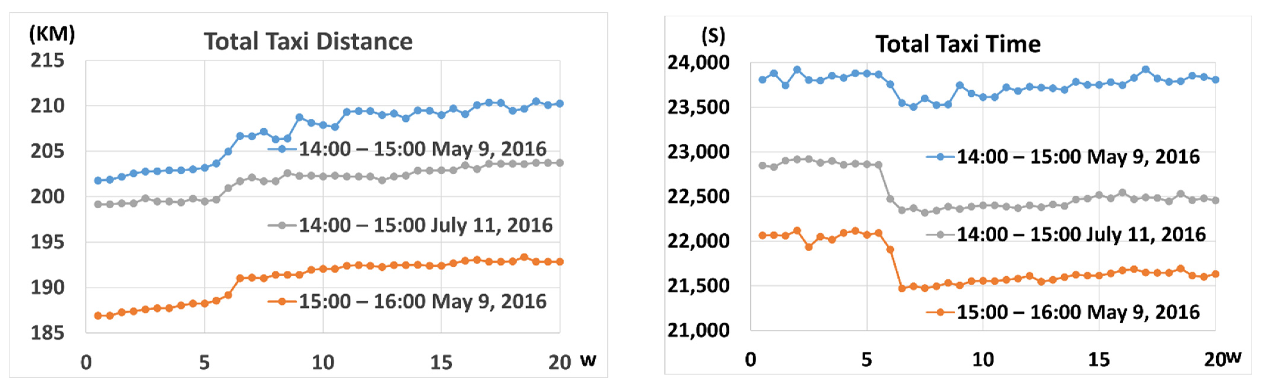
4.2. Result Comparison

The optimized taxiway route and schedule for all the aircraft was obtained from the model results. The observed taxiway route and schedule in the history operation was obtained from the input CARATS Open Data. As the length of each taxiway is fixed, the taxi distance of each aircraft in the observed data and the optimization results can be calculated. The following figures and tables show the comparison results between our optimization results and observed data with or without runway reselection by the runway decider module.

In Figure 9 and Figure 10, each point represents an aircraft in the one-hour time range. The x-axis represents the observed taxi distance in the historical data, while the y-axis represents the taxi distance of the optimized results. An auxiliary line, $y=x$, was used to analyze the comparison results. It was observed that very few aircraft taxi distances become longer; contrarily, most of them decrease.

Table 2. Decreasing rate of total taxi distance.

Items	Values without Runway Reselection	Values with Runway Reselection
Observed total taxi distance	237.55 km	237.55 km
Optimized total taxi distance	214.21 km	193.51 km
Decreasing rate	9.82%	18.54%

shows that the rate of decrease in taxi time of the observed data without runway reselection was 9.82%. It can be observed that the space for optimization is limited, which may be because a smaller distance must be selected as far as possible in the real operation of the airport. The optimization was found to be improved after runway reselection for the take-off aircraft. The total taxi distance was found to decrease by 18.54% compared with the observed results.

The total taxi times of both the observed data and optimized results were calculated as shown in Figure 11 and Figure 12 and

Table 3. Decreasing rate of total taxi time.

Items	Values without Runway Reselection	Values with Runway Reselection
Observed total taxi time	31,240 s	31,240 s
Optimized total taxi time	24,367 s	21,941 s
Decreasing rate	22.00%	29.77%

, similar to the total taxi distance. However, ensuring the accuracy of the calculation of the total taxi time based on the taxi route and schedule was difficult compared with that of the total taxi distance. This is because it is difficult to simulate the change in the taxi speed of the aircraft, especially when the aircraft turns, waits, and pushes back. Only an attempt can be made to ensure that the calculation method of the taxi time is accurate and as close to the observed data as possible. The results obtained reduced the total taxi time by 22.00% without runway reselection and 29.77% with runway reselection. Particularly, the results indicated that optimization of the take-off aircraft was better than that of the landing aircraft. This is compatible with the actual operation because the airport usually assigns higher priority to landing flights.

4.3. Identification of Operation Differences

The results indicated that the developed optimization model improves the airport surface operation. The differences in the operation between the optimized and observed data were identified to obtain a better understanding of the improvement process. A taxiway usage frequency map was used to identify the operation differences. It presents the usage pattern of the optimized taxiway and the differences from the real-world scenario to clearly depict the improvement in the taxi distance and time.

Figure 13 and Figure 14 show that there are several differences between the observed and optimized operations. First, the runway cross strategy has changed. Based on the observed operation using the CARATS Open Data, landing aircraft from runway 22 to Terminal 1 or Terminal 2 primarily use point 4 to cross runway 16R during taxiing, followed by point 1; points 2 and 3 are used less frequently. However, in the optimized operation, it is observed that aircraft primarily use point 1, followed by points 2 and 3, while point 4 is used less frequently. This change may reduce the total taxi distance and waiting time.

The second difference observed was in the congestion area strategy. Based on the analysis of the observed data, it can be observed that point 6 is a congestion area. In the optimized operation, the landing aircraft uses different nodes after exiting a rapid-exit taxiway from the runway, while in the observed operation, the aircraft always uses the same node after exiting the runway. Meanwhile, lesser taxiways are used by the landing aircraft, and it is easier to provide more space for the departure aircraft.

Last, the results indicate that there is no strict rule for direction. Based on the pattern obtained earlier, Tokyo International Airport always applies direction rules on some taxiways to ensure security and efficiency. Considering point 5 as an example, the north side taxiway, K, is always used from left to right, and the south side taxiway, J, is always used from right to left. However, the approach for the optimized result is different. It always uses a closer taxiway to reach an optimized result. Therefore, it does not set taxiway direction or purpose-related rules. When there is a conflict, the optimization system uses a strategy to avoid conflict and ensure safety.

4.4. MILP Weight Parameter Analysis

The objective function discussed in Section 3.4 is a weighted objective function, in which parameter $w$ controls the weight of $ob{j}_{time}$. For a typical global MILP optimization model, the change in $w$ can be directly reflected in the total taxi distance and total taxi time of the final result. However, the MILP model is an optimization model with many planning horizons. The weight parameter can only affect the results of each planning horizon. Therefore, determining the actual impact of the weight parameter on the final results is crucial.

Similar to the implementation settings in Section 4.1, a one-hour time range was set, and the flight information from CARATS Open Data were used as input. Conversely, the optimization model was executed several times for different values of the weight parameter $w$ from 0.5 to 20 in steps of 0.5. This experiment was conducted at different hours and on different dates to ensure the reliability of the results.

Figure 15 shows the results of the weight parameter analysis experiments. Based on the model design, it was assumed that the taxi distance increases with the increase in $w$, whereas the taxi time decreases with the increase in $w$. The results indicate the occurrence of a sudden change when $5\le w\le 7$. Additionally, the total taxi time has a minimum value when $w$ is approximately 7.0, after which it begins to increase. The decrease in the total taxi time was only observed for values of $w$ between 0 and 8; therefore, $w$ must not exceed 8.

4.5. Phenomenon due to Receding Horizon

The weight analysis in Section 4.4 reveals the occurrence of a phenomenon because the approach with RH is an approximation of the global MILP optimal solution and each planning horizon is only 50 s. From the results presented in Section 4.4, we find that if $w$ is larger than 8, the total taxi time begins to increase, although it should decrease in the global optimization model. This occurs because the MILP model with RH cannot predict future congestion and only considers the immediate benefit in the current horizon. We name this phenomenon “Pretend to ignore congestion”.

Figure 16 explains this phenomenon. The blue aircraft is located at its start position of the current planning horizon. When $K=5$, if the MILP model selects the five-step blue route, it will cause a 90 s wait in the runway entrance in the current planning horizon because of runway congestion. However, if it selects the five-step red route, although it has a longer way, the 90 s wait will be avoided, which leads to a better result in terms of the objective function. Thus, the MILP model certainly selects the second choice if the weight of $ob{j}_{time}$ is large. However, the second choice does not mean that congestion will be avoided; the model just pretends to ignore congestion in this horizon.

Two solutions can be considered to reduce the impact of this phenomenon on the results. The first method is directly related to the results presented in Section 4.4, indicating that $w$ must not exceed 8. The second method is to improve $ob{j}_{time}$ in the final objective function, which is already discussed in Section 3.4. However, the latter method only works on runway congestion, not on taxiway congestion. Because taxiway congestion does not occur at the end of the aircraft taxi process, it is impossible to add a long virtual waiting time.

4.6. Gate Re-Assignment and Analysis of Airline–Terminal Relationships

The selection of the aircraft take-off and landing runways is largely affected by the air routes. The flight route in the air space was changed by a runway decider in this study. As this study was only based on surface optimization, the gate and terminal of the flight can be re-assigned to achieve a similar optimization result without changing the selection of the runway.

Table 4. Distribution of airlines in each terminal before and after gate re-assignment.

Terminal		T1		T2		T3
Airlines		JAL, Skymark	ANA	JAL, Skymark	ANA	All
Observed data	Take-off	17	0	0	11	3
	Landing	13	0	0	20	5
After re-assignment	Take-off	4	4	13	7	3
	Landing	8	13	5	7	5

shows the distribution of the airlines in each terminal before and after the gate re-assignment. Based on the operation mode of Tokyo International Airport before 2020, for domestic flights, Terminal 1 is used by JAL, Skymark Airlines, and others, while Terminal 2 is used by ANA and others. Based on the taxi distance between the different runways and terminals, the terminals can be re-assigned for unsuitable flights.

The domestic flights ANA and JAL are assigned to both Terminals 1 and 2 after gate re-assignment.

Table 5. Decreasing rate comparison with runway reselection and gate re-assignment.

	Taxi Distance			Taxi Time
	Take-Off	Landing	Total	Take-Off	Landing	Total
Optimized result	11.15%	9.03%	9.82%	32.29%	13.08%	22.00%
Optimized result with runway reselection	34.12%	9.16%	18.54%	48.56%	13.49%	29.77%
Optimized result with gate re-assignment	35.7 6%	26.07%	29.71%	47.22%	28.78%	37.34%

shows that the optimized results with gate re-assignment are better than the optimized results without gate re-assignment. In fact, gate re-assignment results in a 29.71% reduction in the total taxi distance and 37.34% reduction in the total taxi time compared with the observed data. The results of the take-off aircraft taxi time were slightly worse than those of the runway reselection optimization, but the overall results were better than those of the runway reselection optimization.

In Section 4.2, Figure 11 and Figure 12 are used to show the optimization results of each aircraft. It was found that the optimization for take-off aircraft is better than that for landing aircraft, and there is only limited space for optimization of the total taxi time of landing aircraft. Table 5 shows that gate re-assignment leads to a better optimization for landing aircraft compared with optimization with runway reselection.

Although gate re-assignment does not affect the airspace side, this analysis disregards the following facts. The gate assignment of the aircraft involves the connection of the preceding and following aircraft, but the take-off and landing aircraft in this study are independent and lose their connection data. Because flights with only a 1 h time range were considered, we do not consider the gate occupation by previous and subsequent aircraft and cannot track the same numbers of arrival and departure aircraft of the same airline in the same terminal. Further, the actual gate assignment is completed very early and cannot be based on real-time flight operation situations, whereas this analysis was based on real-time data. Therefore, the analysis presented in this section may lead to overestimation.

5. Conclusions

This study developed a dynamic optimization model of surface operation to apply for the Tokyo International Airport. It solves the problems of runway crossing operations, multi-runways, and multi-terminal operations. The obtained results indicate that the developed model reduces the taxi distance by 18.54% and taxi time by 29.77% compared with the observed data. This model can also identify the operation difference between optimization and reality by comparing the taxiway usage patterns. A better understanding of the improvement process is obtained from this comparison; for example, the runway cross strategy and taxiway direction rule are changed in the optimized operation. Additionally, it is observed that factors such as the MILP weights and airline–terminal relationships can affect the optimization result.

The results of this study can bring improvements to real airport surface operations. The comparison between the optimization results and the observed operations can offer suggestions to the air traffic control, such as the strategy of runway cross points selection and the taxiway direction rules. The re-selection of runway and the cooperation of terminal usage between airlines can improve the ground operation efficiency of the airport. Simultaneously, the dynamic model with a time window makes feasible the idea of applying the optimization model to practical operation.

The developed model has certain limitations. It cannot accurately simulate the speed change of the aircraft, and the comparison of the computed total taxi time with that of the observed data is not very accurate. Gate re-assignment in Section 4.6 shows a good result and presents an adequate outline of the airline–terminal relationships, but it lacks the real data generated by gate occupation in the terminal; owing to this, the results may be overestimated. In the future, the developed model can be enhanced by considering airspace side operations as the choice of runway on the ground and the landing time are closely related to the air route. Furthermore, this study focuses on optimizing the total taxi distance and time, which are direct indicators. Further benefits and indicators to the stakeholders can be analyzed in the future, such as the improvement of the flight punctuality, improvement of passenger waiting time, and impact of different taxi waiting times on fuel consumption and CO₂ emissions.

References

1. Simaiakis, I.; Khadilkar, H.; Balakrishnan, H.; Reynolds, T.G.; Hansman, R.J. Demonstration of reduced airport congestion through pushback rate control. Transp. Res. Part A Policy Pract. 2014, 66, 251–267. [Google Scholar] [CrossRef]
2. Gudmundsson, S.V.; Cattaneo, M.; Redondi, R. Forecasting temporal world recovery in air transport markets in the presence of large economic shocks: The case of COVID-19. J. Air Transp. Manag. 2021, 91, 102007. [Google Scholar] [CrossRef]
3. Airports Council International. Annual World Airport Traffic Report 2020; Airports Council International: Montreal, QC, Canada, 2020. [Google Scholar]
4. Watabe, Y.; Noguchi, T. Site-investigation and geotechnical design of D-runway construction in Tokyo Haneda airport. Soils Found. 2011, 51, 1003–1018. [Google Scholar] [CrossRef] [Green Version]
5. Gotteland, J.B.; Durand, N. Genetic algorithms applied to airport ground traffic optimization. In Proceedings of the 2003 Congress on Evolutionary Computation, CEC ’03, Canberra, Australia, 8–12 December 2003; Volume 1, pp. 544–551. [Google Scholar] [CrossRef] [Green Version]
6. Atkin, J.A.D.; Burke, E.K.; Ravizza, S. The airport ground movement problem: Past and current research and future directions. In Proceedings of the 4th International Conference on Research in Air Transportation (ICRAT), Budapest, Hungary, 1–4 June 2010; pp. 131–138. [Google Scholar]
7. Daş, G.S.; Gzara, F.; Stützle, T. A review on airport gate assignment problems: Single versus multi objective approaches. Omega 2020, 92, 102146. [Google Scholar] [CrossRef]
8. Smeltink, J.W.; Soomer, M.J.; de Waal, P.R.; van der Mei, R.D. An Optimisation Model for Airport Taxi Scheduling. In Proceedings of the INFORMS Annual Meeting, Denver, CO, USA, 24–27 October 2004. [Google Scholar]
9. Pesic, B.; Durand, N.; Alliot, J.-M. Aircraft Ground Traffic Optimisation Using a Genetic Algorithm. In Proceedings of the Genetic and Evolutionary Computation Conference, San Francisco, CA, USA, 7–11 July 2001. [Google Scholar]
10. Ravizza, S.; Atkin, J.A.D.; Burke, E.K. A more realistic approach for airport ground movement optimisation with stand holding. J. Sched. 2014, 17, 507–520. [Google Scholar] [CrossRef] [Green Version]
11. Brownlee, A.E.I.; Weiszer, M.; Chen, J.; Ravizza, S.; Woodward, J.R.; Burke, E.K. A fuzzy approach to addressing uncertainty in Airport Ground Movement optimisation. Transp. Res. Part C Emerg. Technol. 2018, 92, 150–175. [Google Scholar] [CrossRef]
12. Chen, J.; Weiszer, M.; Locatelli, G.; Ravizza, S.; Atkin, J.A.; Stewart, P.; Burke, E.K. Toward a More Realistic, Cost-Effective, and Greener Ground Movement Through Active Routing: A Multiobjective Shortest Path Approach. IEEE Trans. Intell. Transp. Syst. 2016, 17, 3524–3540. [Google Scholar] [CrossRef] [Green Version]
13. Clare, G.; Richards, A.G. Optimization of taxiway routing and runway scheduling. IEEE Trans. Intell. Transp. Syst. 2011, 12, 1000–1013. [Google Scholar] [CrossRef]
14. Behrends, J.A.; Usher, J.M. Aircraft gate assignment: Using a deterministic approach for integrating freight movement and aircraft taxiing. Comput. Ind. Eng. 2016, 102, 44–57. [Google Scholar] [CrossRef]
15. Yu, C.; Zhang, D.; Henry Lau, H.Y.K. A heuristic approach for solving an integrated gate reassignment and taxi scheduling problem. J. Air Transp. Manag. 2017, 62, 189–196. [Google Scholar] [CrossRef]
16. MLIT Collaborative Actions for Renovation of Air Traffic Systems (CARATS). Available online: http://www.mlit.go.jp/common/001046514.pdf (accessed on 1 June 2020).
17. Google earth V 7.3.3.7786 Tokyo International Airport, Tokyo, Japan. 35° 33′24.11″ N, 139° 45′48.42″ E, Eye alt 10.35 km. Available online: http://earth.google.com (accessed on 30 June 2020).
18. Bellingham, J.; Kuwata, Y.; How, J. Stable receding horizon trajectory control for complex environments. In Proceedings of the AIAA Guidance, Navigation, and Control Conference and Exhibit, Austin, TX, USA, 11–14 August 2003; American Institute of Aeronautics and Astronautics: Reston, VA, USA, 2003. [Google Scholar]
19. Schouwenaars, T.; De Moor, B.; Feron, E.; How, J. Mixed integer programming for multi-vehicle path planning. In Proceedings of the 2001 European Control Conference (ECC), Porto, Portugal, 4–7 September 2001; pp. 2603–2608. [Google Scholar] [CrossRef]
20. Floyd, R.W. Algorithm 97: Shortest path. Commun. ACM 1962, 5, 345. [Google Scholar] [CrossRef]
21. Clare, G.; Richards, A.; Sharma, S. Receding Horizon, iterative optimization of taxiway routing and runway scheduling. In Proceedings of the AIAA Guidance, Navigation, and Control Conference and Exhibit, Chicago, IL, USA, 10–13 August 2009. [Google Scholar] [CrossRef]
22. Bellingham, J.; Richards, A.; How, J.P. Receding horizon control of autonomous aerial vehicles. In Proceedings of the 2002 American Control Conference (IEEE Cat. No. CH37301), Anchorage, AK, USA, 8–10 May 2002; pp. 3741–3746. [Google Scholar] [CrossRef]
Figure 1. Location of runways and terminals at the Tokyo International Airport. Source: Google Earth (2020) [17].
Aerospace 09 00145 g001
Figure 2. Taxiway selection patterns. (a) Take-off. (b) Landing. (Source: CARATS Open Data on 9 May 2016).
Aerospace 09 00145 g002
Figure 3. Graph model of Tokyo International Airport.
Aerospace 09 00145 g003
Figure 4. Example of virtual pushback node.
Aerospace 09 00145 g004
Figure 5. Runway virtual nodes and cross nodes.
Aerospace 09 00145 g005
Figure 6. Two types of aircraft conflict on a taxiway. (a) 1st type conflict at each node. (b) 2nd type conflict at each edge.
Aerospace 09 00145 g006
Figure 7. Runway decider workflow.
Aerospace 09 00145 g007
Figure 8. Model implementation and analysis flow.
Aerospace 09 00145 g008
Figure 9. Result comparison of total taxi distance without runway reselection.
Aerospace 09 00145 g009
Figure 10. Result comparison of total taxi distance with runway reselection.
Aerospace 09 00145 g010
Figure 11. Result comparison of total taxi time without runway reselection.
Aerospace 09 00145 g011
Figure 12. Result comparison of total taxi time with runway reselection.
Aerospace 09 00145 g012
Figure 13. Taxiway usage frequency map of landing aircraft. (a) Observed data. (b) Optimized result.
Aerospace 09 00145 g013
Figure 14. Taxiway usage frequency map of take-off aircraft. (a) Observed data. (b) Optimized result.
Aerospace 09 00145 g014
Figure 15. MILP weight parameter analysis result.
Aerospace 09 00145 g015
Figure 16. “Pretend to ignore congestion” in MILP with RH.
Aerospace 09 00145 g016