
Satellite Cluster Formation Reconfiguration Based on the Bifurcating Potential Field


Abstract
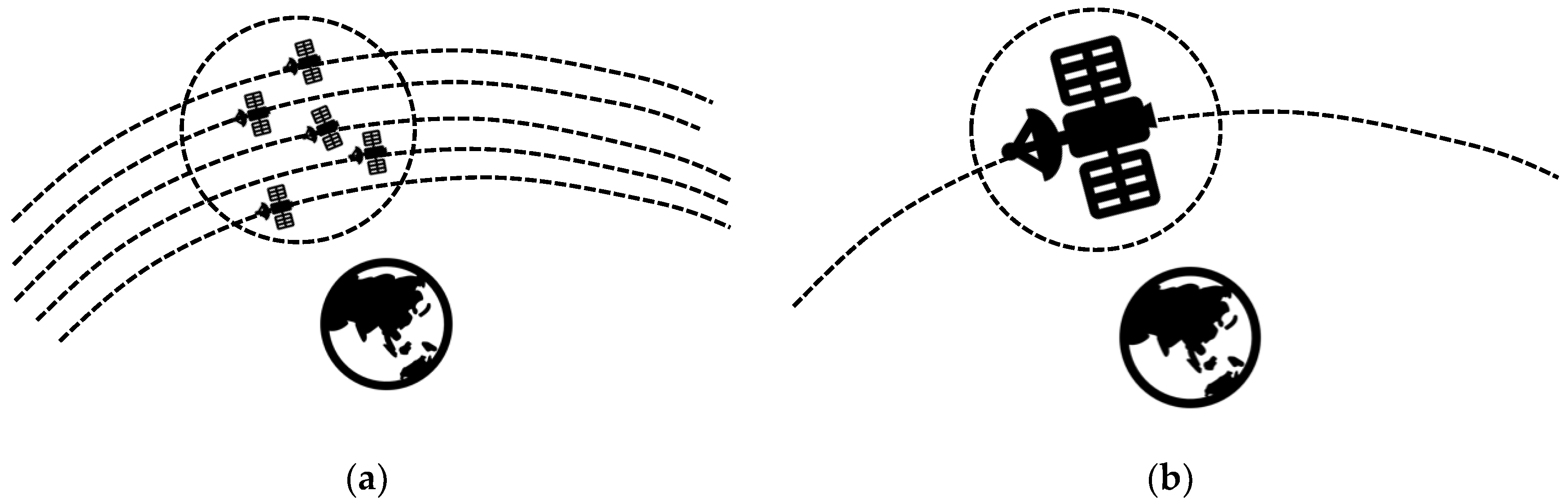
:1. Introduction
2. Materials and Methods
2.1. The Five Descriptive Elements of Satellite Cluster
2.1.1. Cluster Size
2.1.2. Cluster Movement
2.1.3. Outer Boundary of the Cluster
2.1.4. Inner Boundary of the Cluster
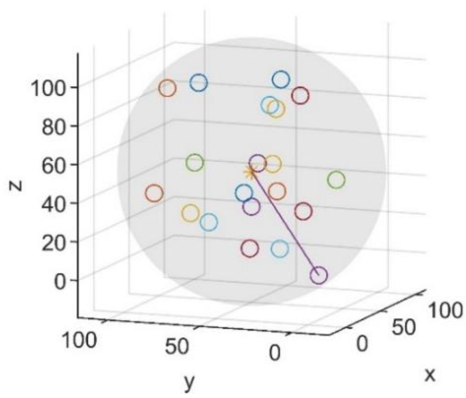
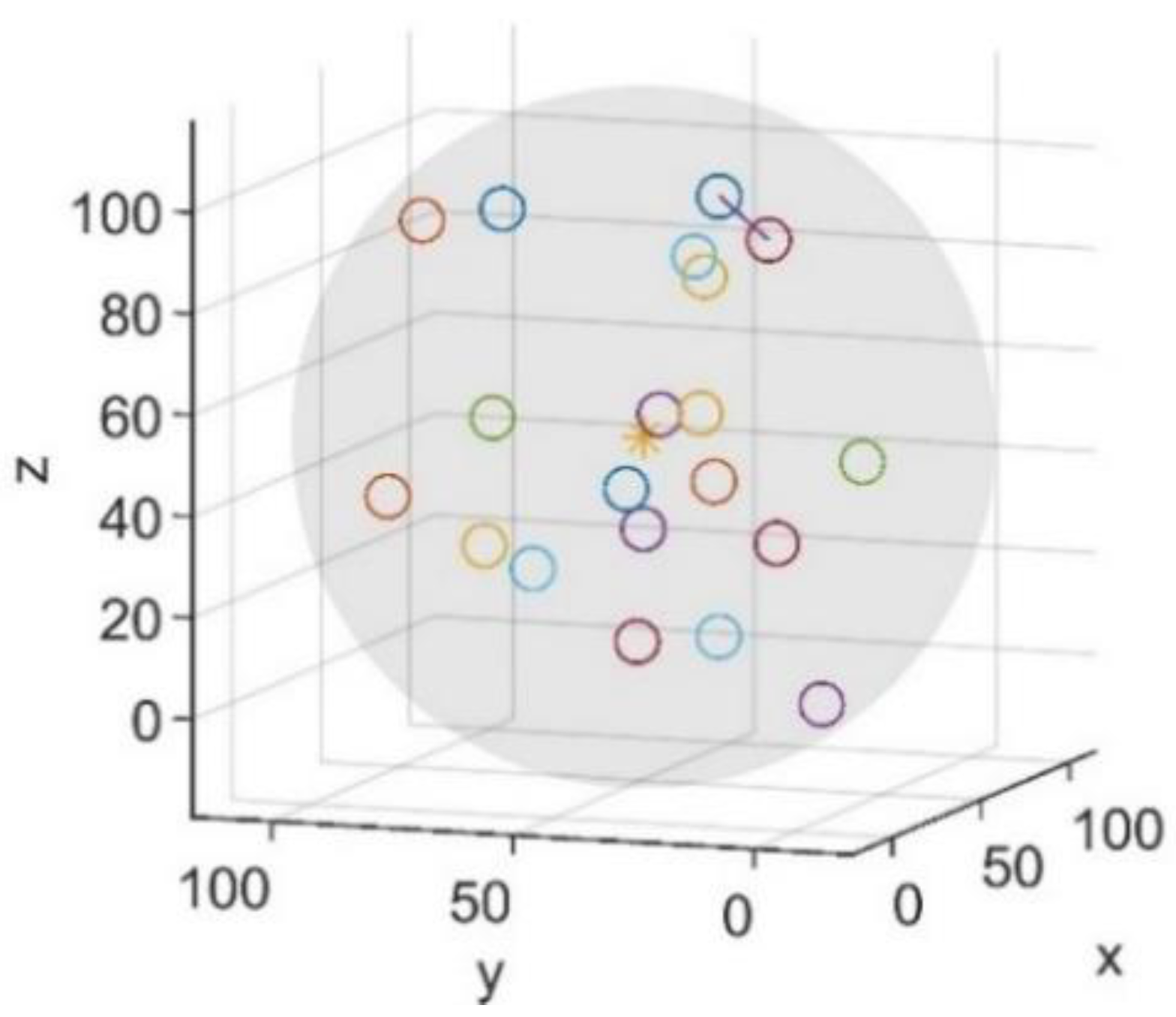
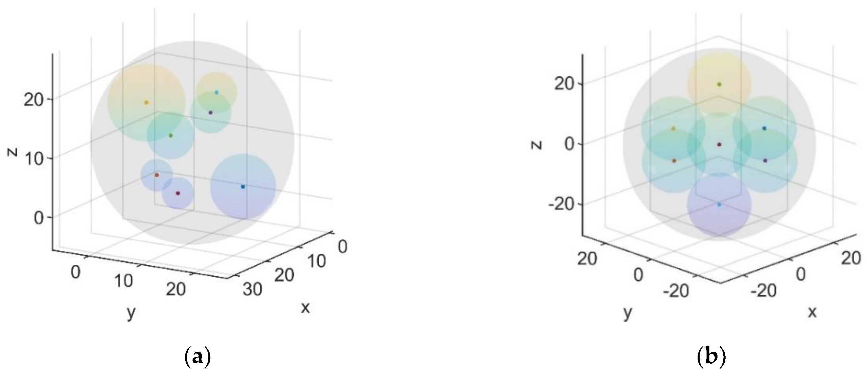
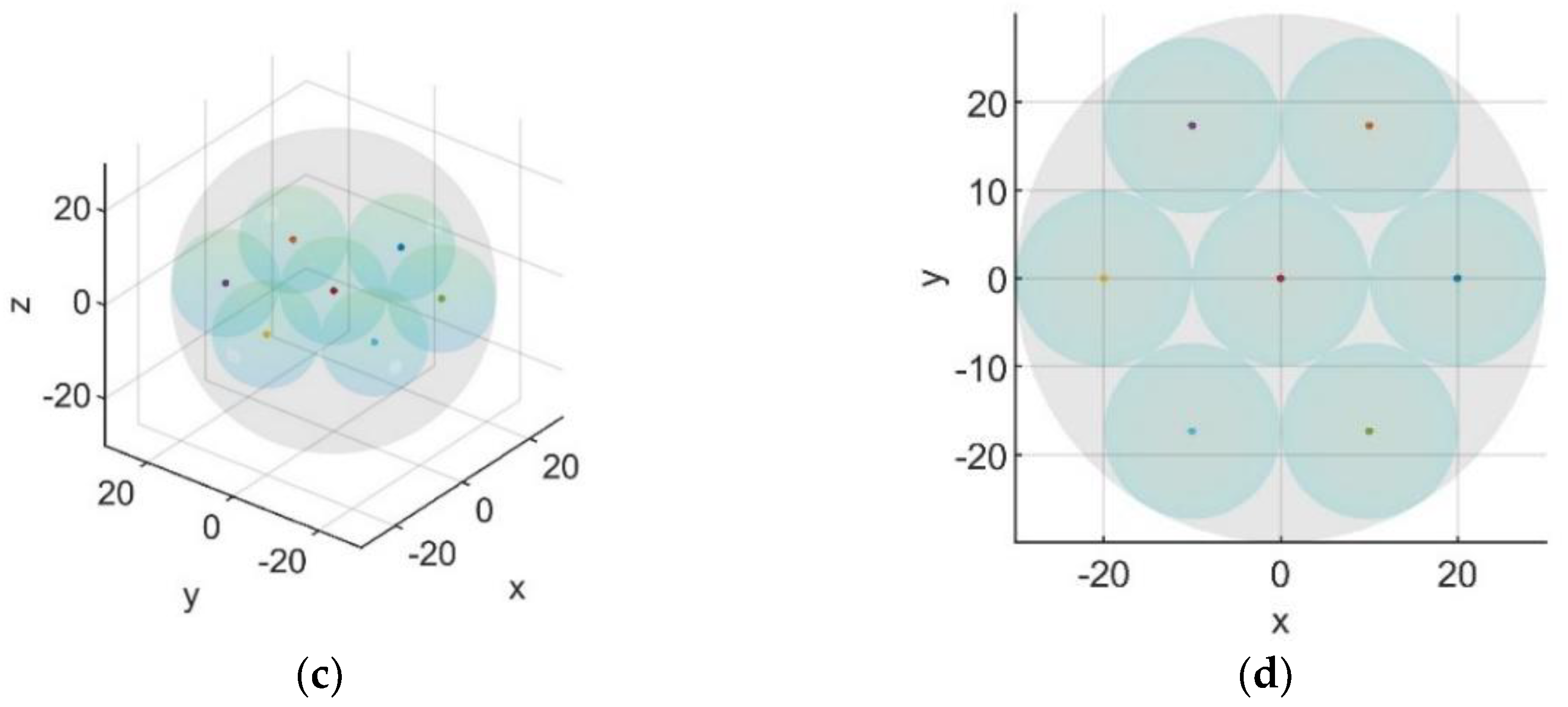
2.1.5. Distribution Uniformity of the Cluster
- The radius of each member satellite’s monopolized sphere is calculated according to the distance between each member satellite:
- 2
- Calculate the volume of each member satellite’s monopolized sphere:
- 3
- Calculate the radius of circumscribed sphere of all satellites’ monopolized spheres:
- 4
- Calculate the volume of the circumscribed sphere:
- 5
- Finally, the distribution uniformity of the cluster is calculated by Equation (5).
2.2. Formation Control Algorithm
2.2.1. Dynamic Model of Satellite Cluster
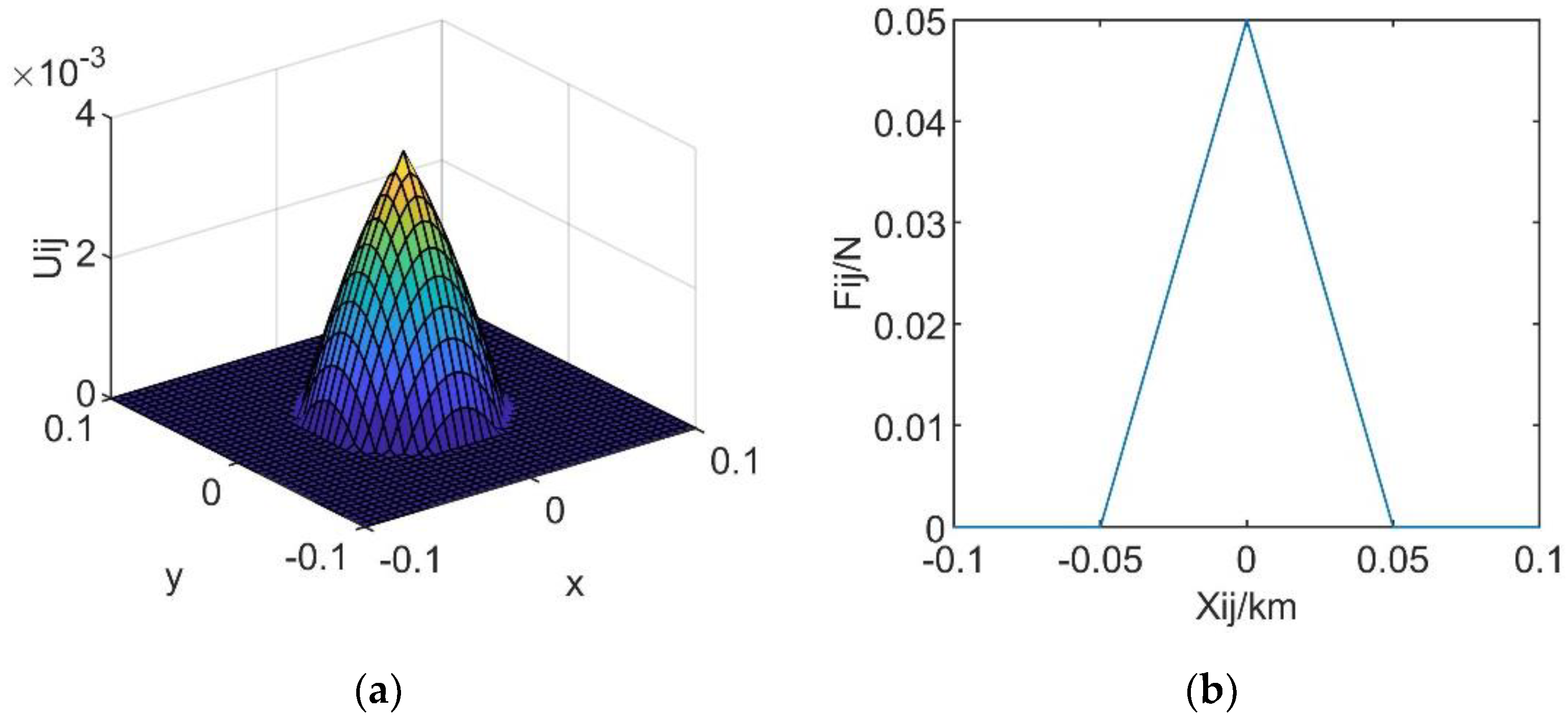
2.2.2. Collision Avoidance Potential Function
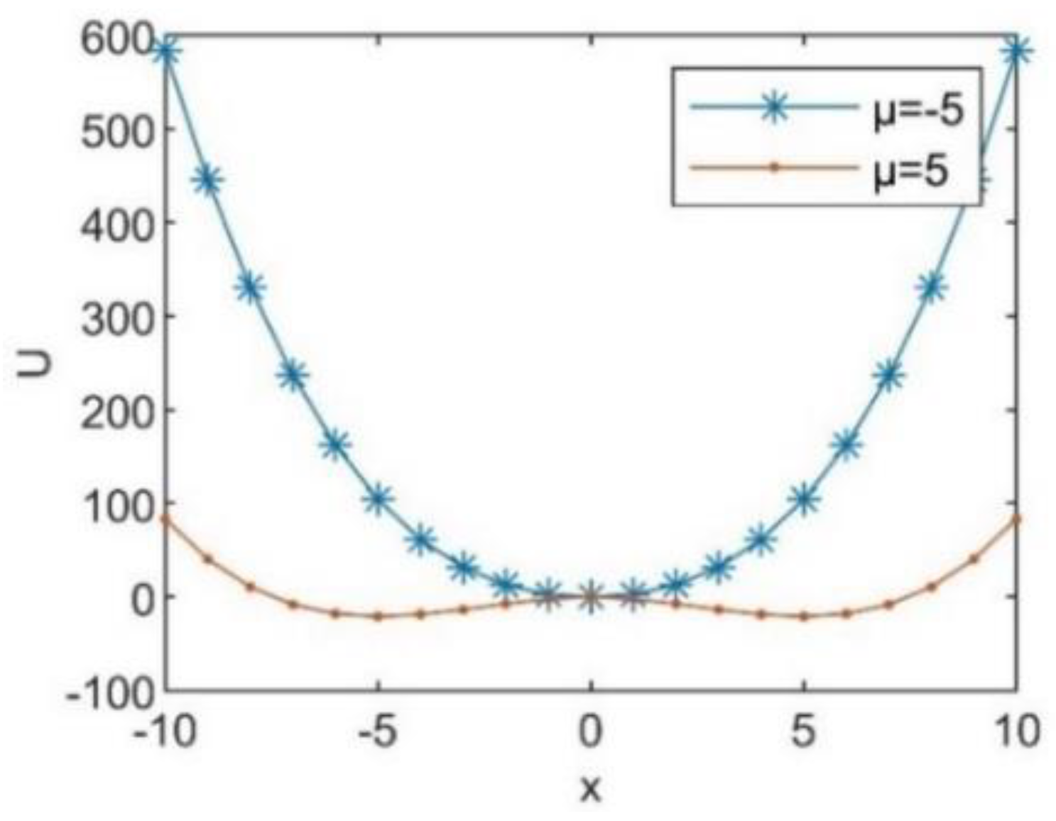
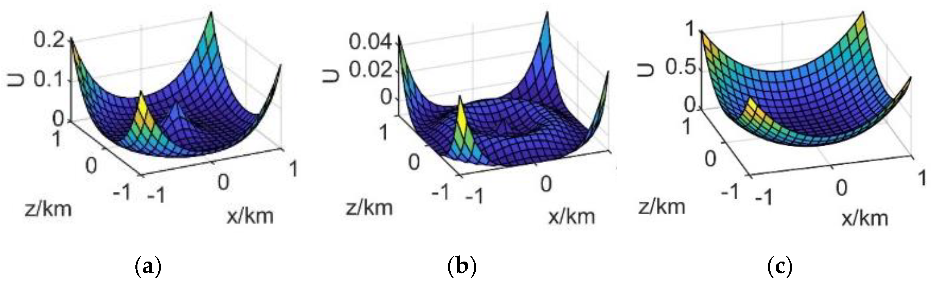
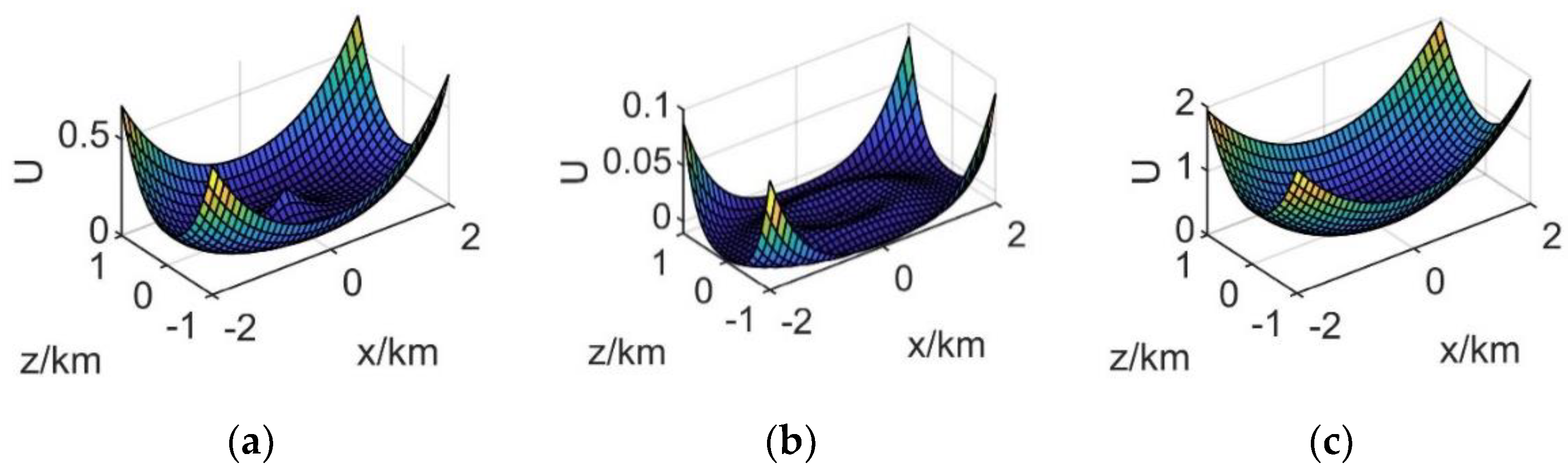
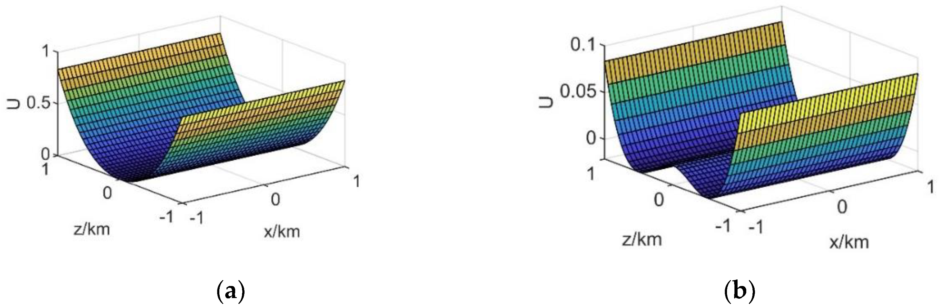
2.2.3. Bifurcating Potential Function
3. Results and Discussion
3.1. Formation Configuration
3.1.1. Line and Double Line Formation
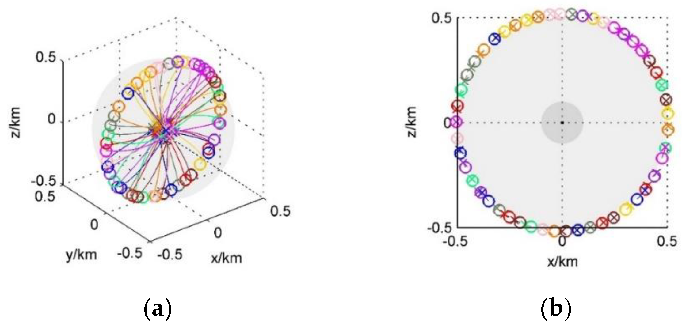
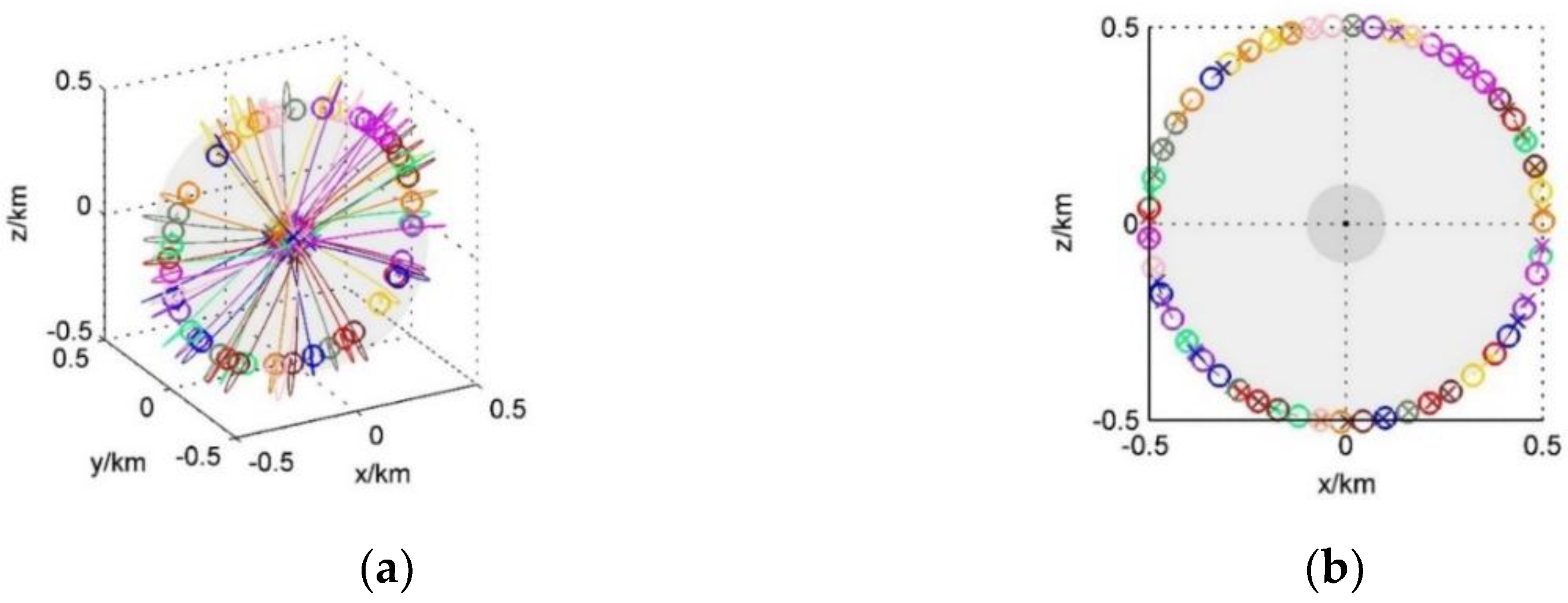
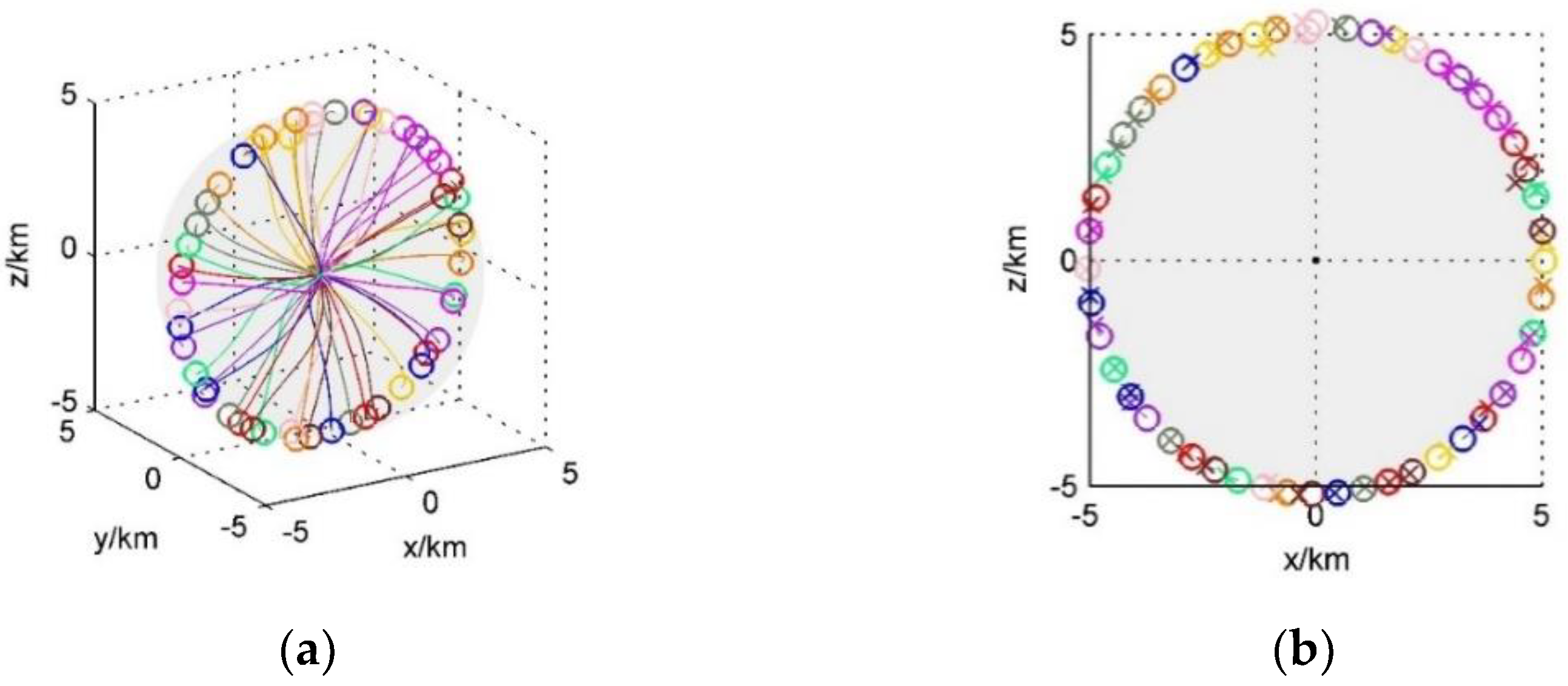
3.1.2. Circle Formation
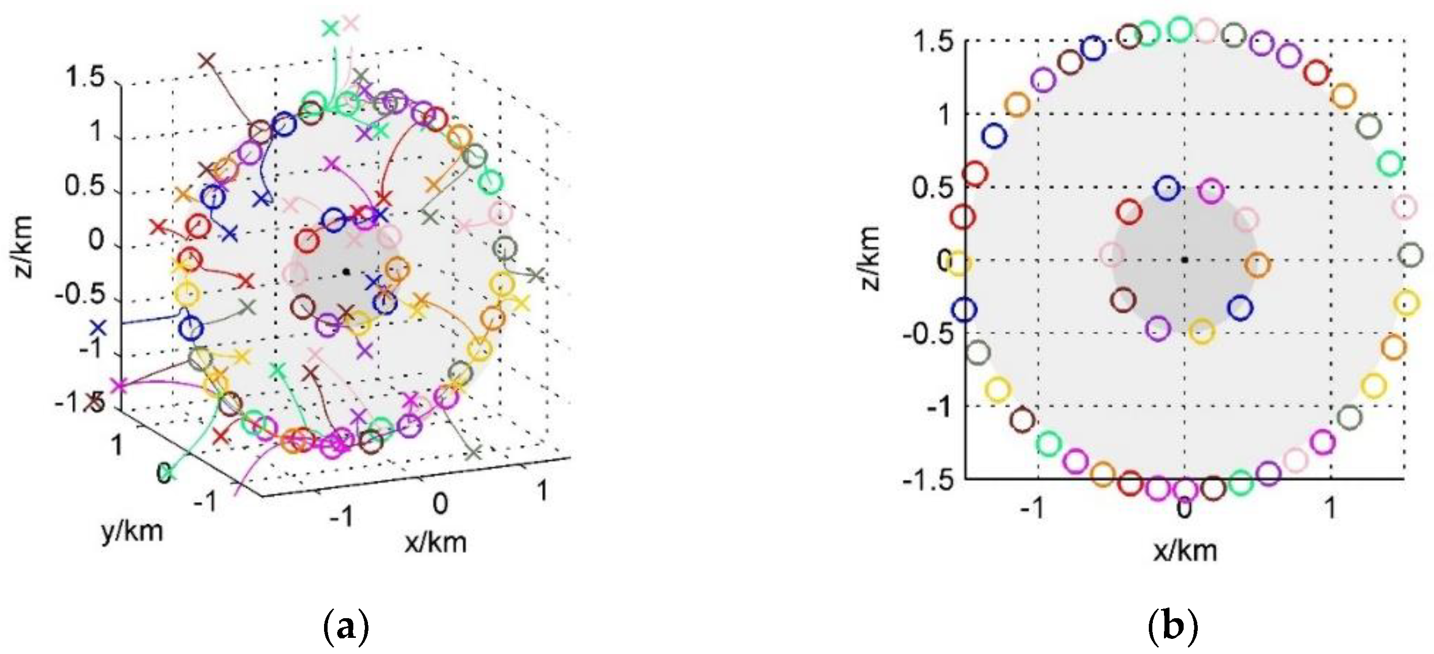
3.1.3. Concentric Double Circle Formation
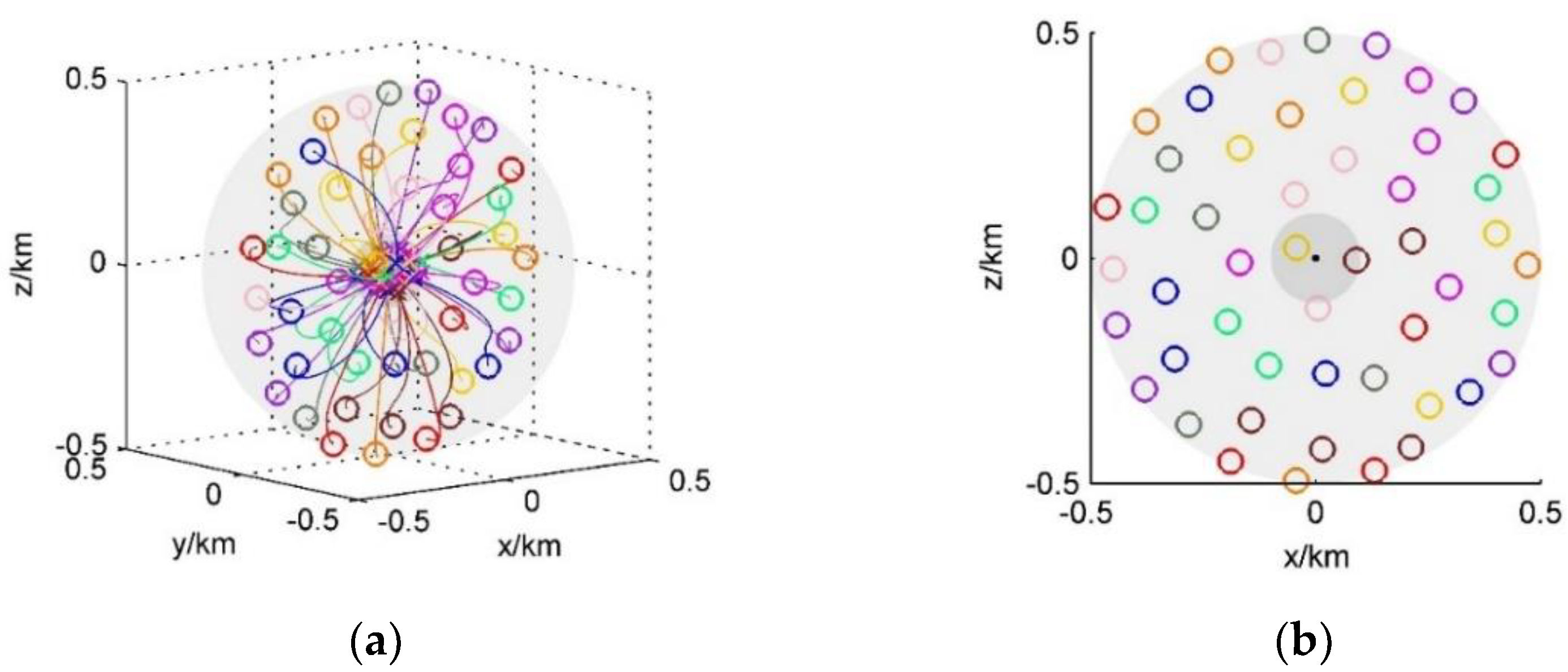
3.1.4. Disk Formation
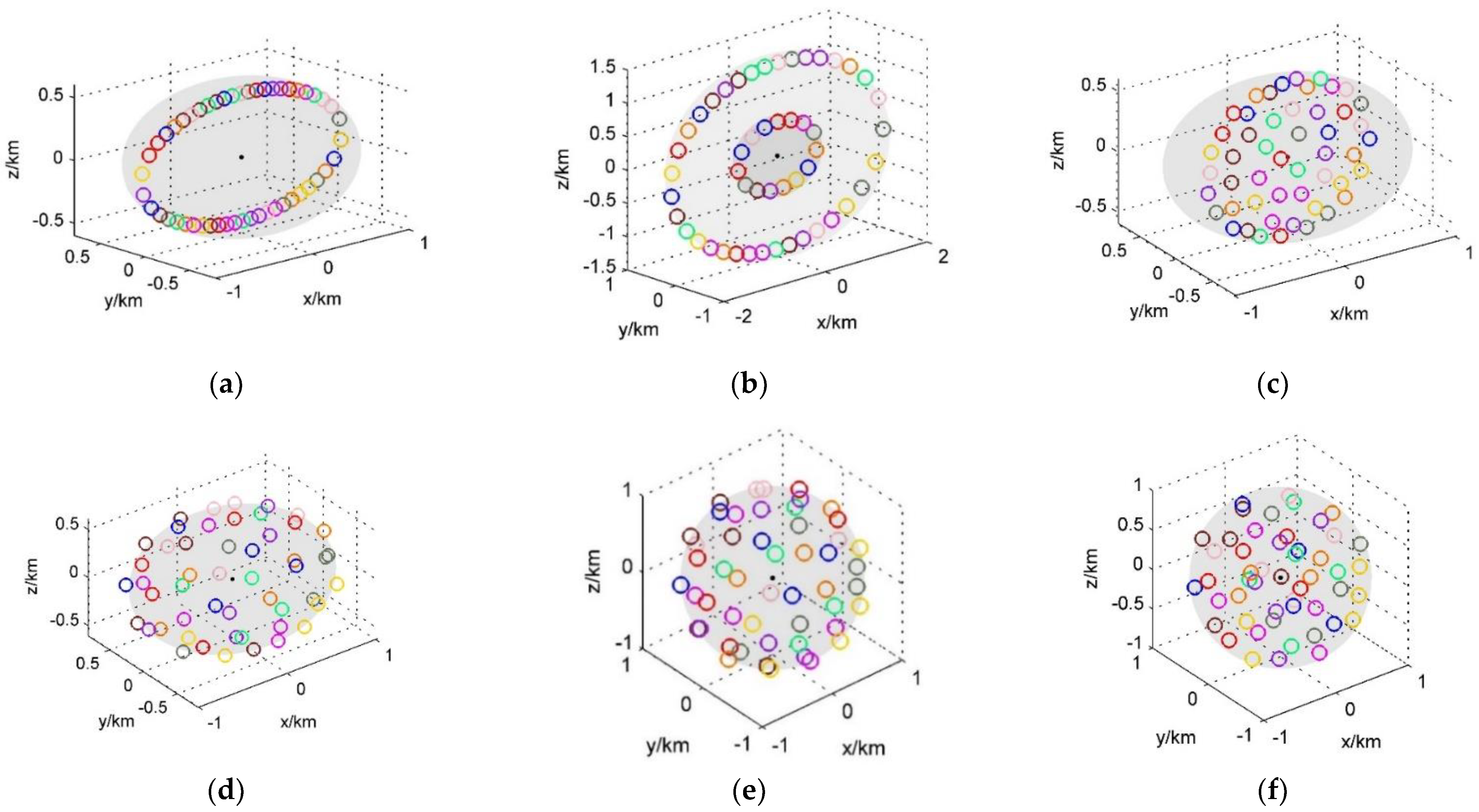
3.1.5. A Variety of Formations
- The distribution uniformity of in-plane formation is lower than that of stereo formation;
- Among in-plane formations, the distribution uniformity of linear formation is lower than that of disk formation;
- The distribution uniformity of monolayer formation is lower than that of bilayer formation.
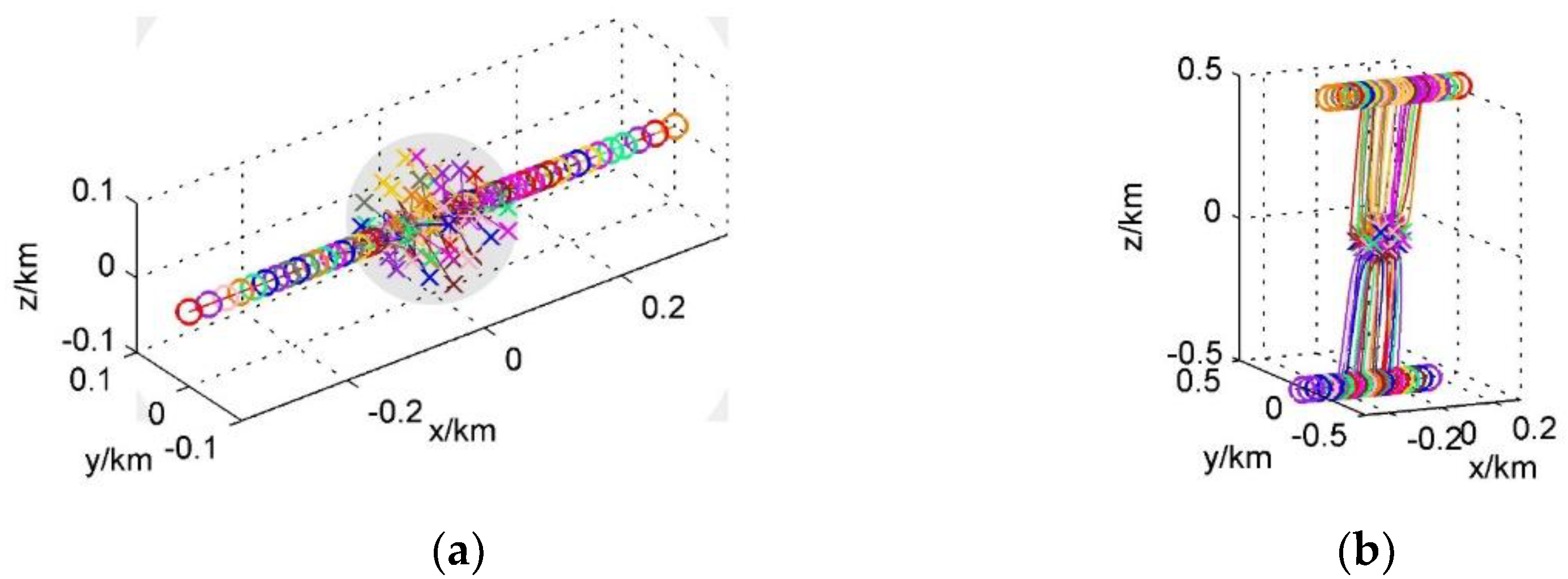
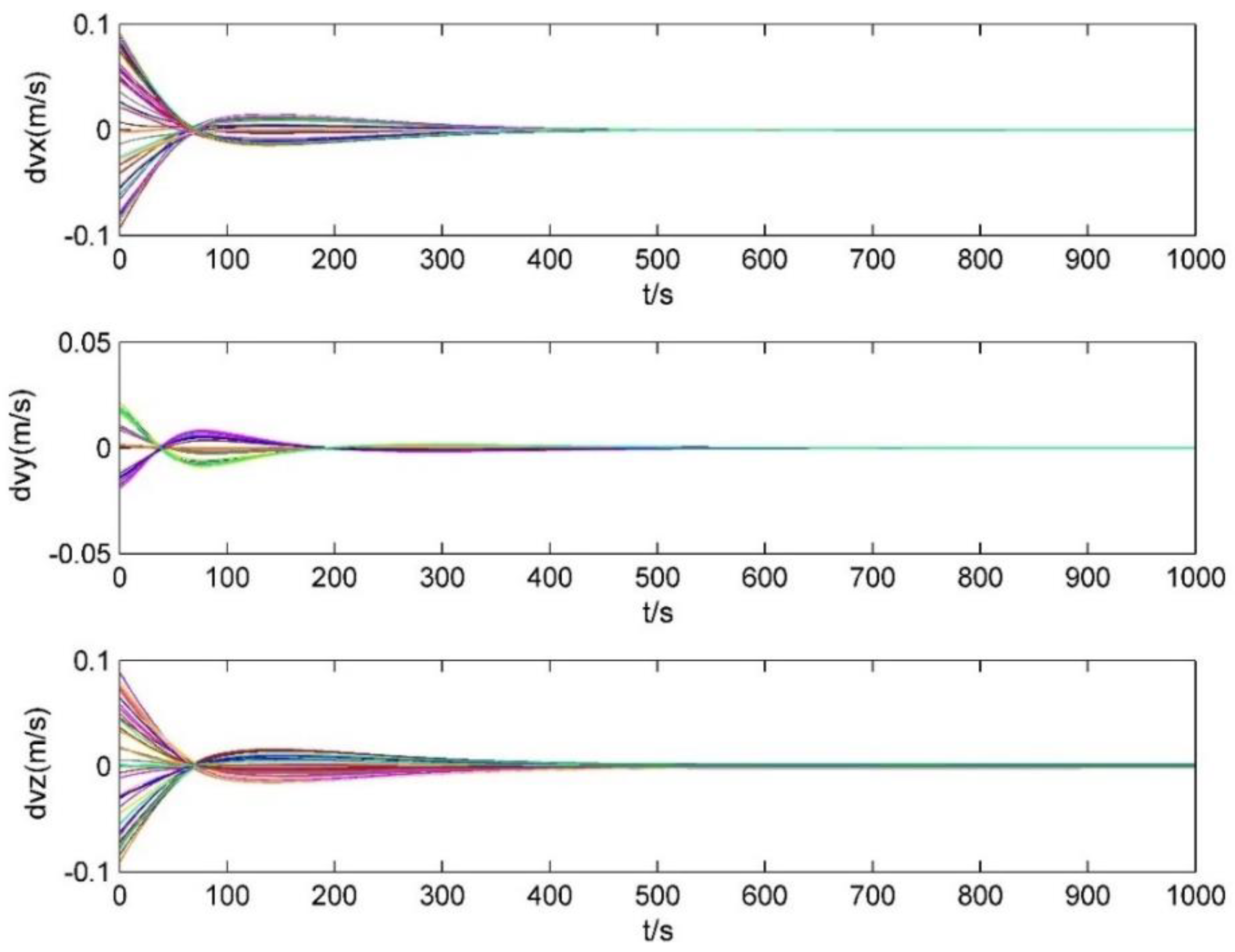
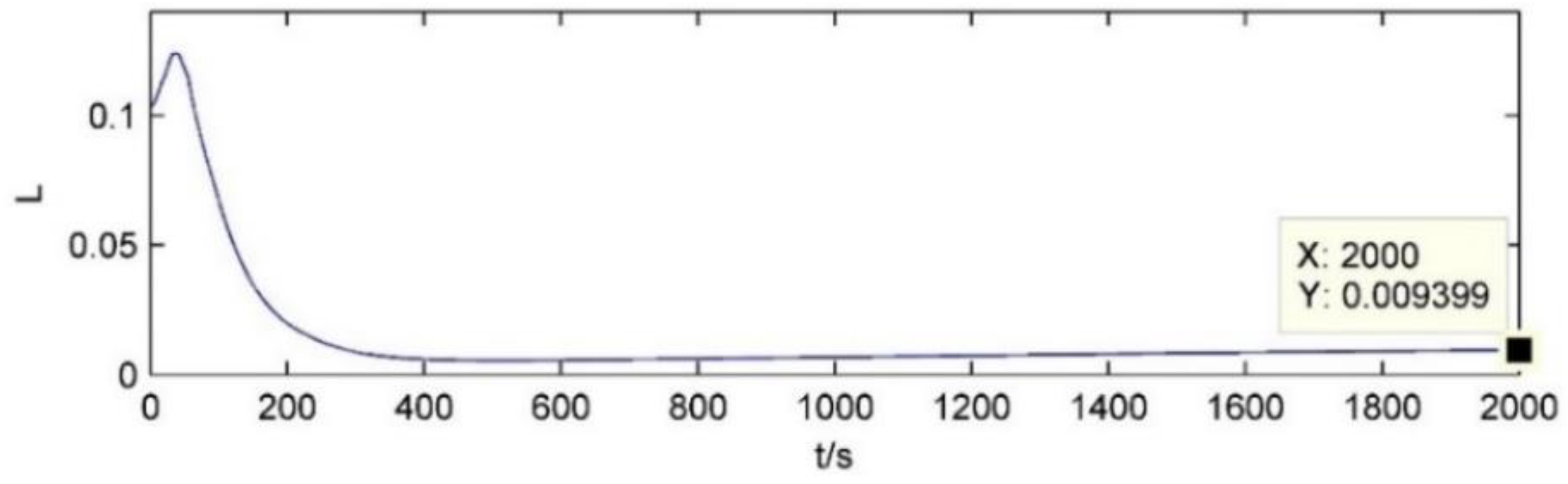
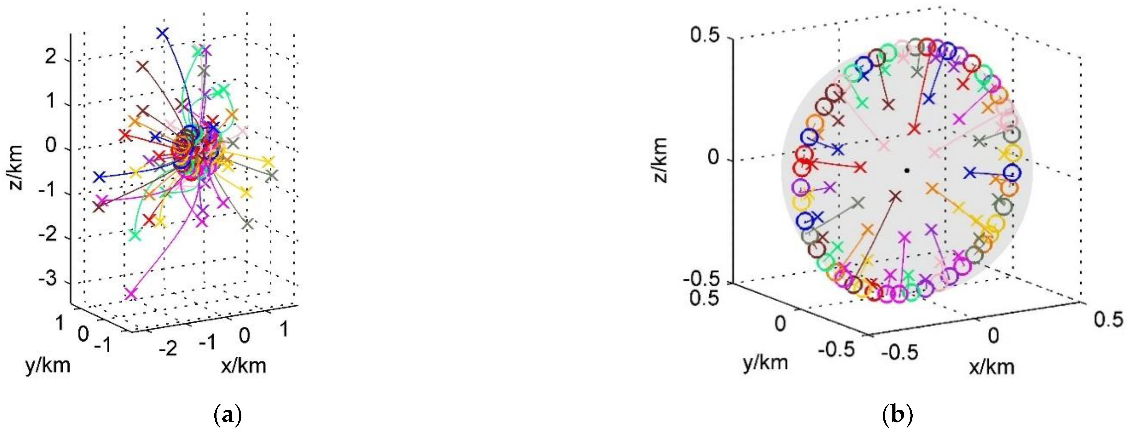
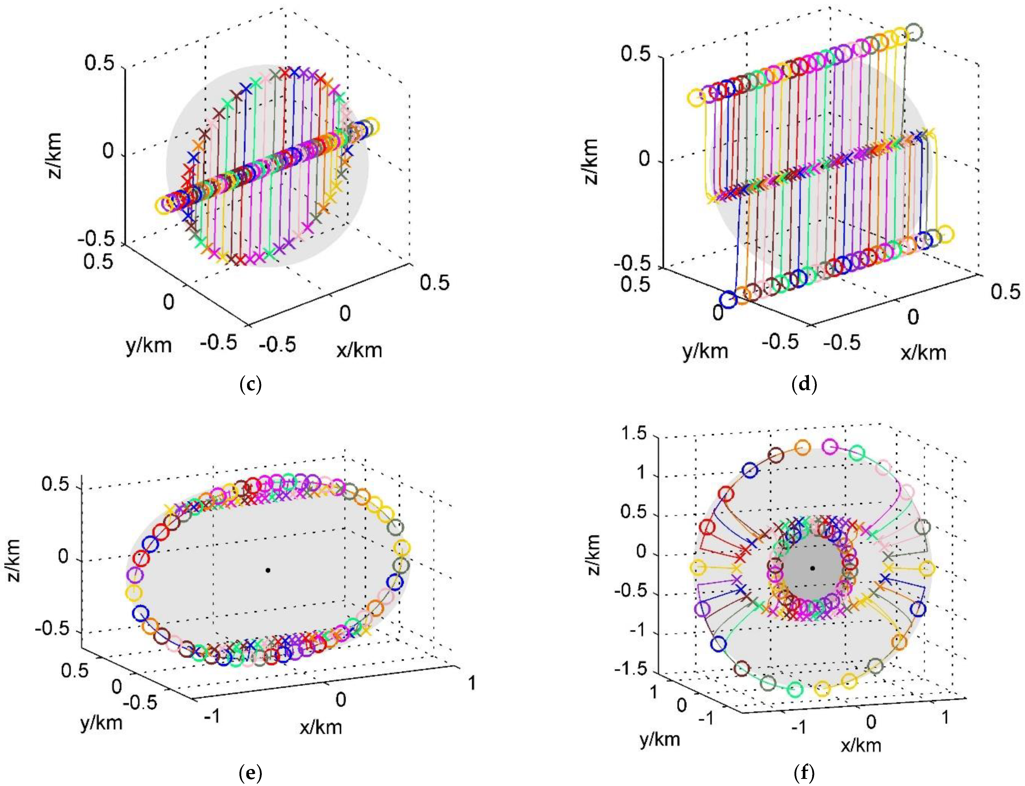
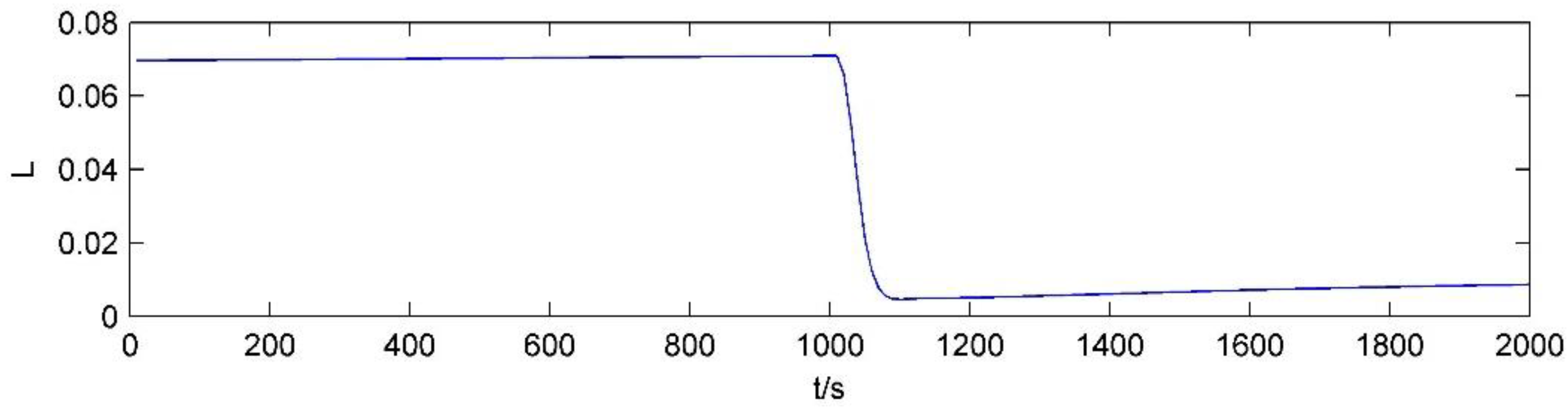
3.2. Formation Reconfiguration
4. Conclusions
Author Contributions
Funding
Institutional Review Board Statement
Informed Consent Statement
Data Availability Statement
Conflicts of Interest
References
- Mazal, L.; Gurfil, P. Closed-Loop Distance-Keeping for Long-Term Satellite Cluster Flight. Acta Astronaut. 2014, 94, 73–82. [Google Scholar] [CrossRef]
- Alvarez, J.; Walls, B. Constellations, Clusters, and Communication Technology: Expanding Small Satellite Access to Space. In Proceedings of the 2016 IEEE Aerospace Conference, Big Sky, MT, USA, 5–12 March 2016; pp. 1–11. [Google Scholar]
- Edlerman, E.; Gurfil, P. Cluster-Keeping Algorithms for the Satellite Swarm Sensor Network Project. J. Spacecr. Rocket. 2019, 56, 649–663. [Google Scholar] [CrossRef]
- Manchester, Z.; Peck, M.; Filo, A. KickSat: A Crowd-Funded Mission to Demonstrate the World’s Smallest Spacecraft. In Proceedings of the 27th Small Satellite Conference, Logan, UT, USA, 12–15 August 2013. [Google Scholar]
- Boshuizen, C.; Mason, J.; Klupar, P.; Spanhake, S. Results from the Planet Labs Flock Constellation. In Proceedings of the 28th Small Satellite Conference, Logan, UT, USA, 2–7 August 2014. [Google Scholar]
- Hegel, D. FlexCore: Low-Cost Attitude Determination and Control Enabling High-Performance Small Spacecraft. In Proceedings of the 30th Small Satellite Conference, Logan, UT, USA, 6–11 August 2016. [Google Scholar]
- Sanchez, H.; Mcintosh, D.; Cannon, H.; Pires, C.; Sullivan, J.; D’Amico, S.; O’Connor, B. Starling1: Swarm Technology Demonstration. In Proceedings of the 32th Small Satellite Conference, Logan, UT, USA, 4–9 August 2018. [Google Scholar]
- Hadaegh, F.Y.; Chung, S.-J.; Manohara, H.M. On Development of 100-Gram-Class Spacecraft for Swarm Applications. IEEE Syst. J. 2016, 10, 673–684. [Google Scholar] [CrossRef] [Green Version]
- Truszkowski, W.; Hinchey, M.; Rash, J.; Rouff, C. NASA’s Swarm Missions: The Challenge of Building Autonomous Software. IT Prof. 2004, 6, 47–52. [Google Scholar] [CrossRef]
- Engelen, S.; Verhoeven, C.J.M.; Bentum, M.J. Olfar, a Radio Telescope Based on Nano-Satellites in Moon Orbit. In Proceedings of the 24th Small Satellite Conference, Logan, UT, USA, 9–12 August 2010. [Google Scholar]
- Bentum, M.J.; Verma, M.K.; Rajan, R.T.; Boonstra, A.J.; Verhoeven, C.J.M.; Gill, E.K.A.; van der Veen, A.J.; Falcke, H.; Wolt, M.K.; Monna, B.; et al. A Roadmap towards a Space-Based Radio Telescope for Ultra-Low Frequency Radio Astronomy. Adv. Space Res. 2020, 65, 856–867. [Google Scholar] [CrossRef] [Green Version]
- Yang, L.; Guo, J.; Fan, C.; Song, X.; Wu, S.; Zhao, Y. The Design and Experiment of Stardust Femto-Satellite. Acta Astronaut. 2020, 174, 72–81. [Google Scholar] [CrossRef]
- Wu, S.; Chen, W.; Zhang, Y.; Baan, W.; An, T. SULFRO: A Swarm of Nano-/Micro-Satellite at SE L2 for Space Ultra-Low Frequency Radio Observatory. In Proceedings of the 28th Small Satellite Conference, Logan, UT, USA, 2–7 August 2014. [Google Scholar]
- Levchenko, I.; Bazaka, K.; Ding, Y.; Raitses, Y.; Mazouffre, S.; Henning, T.; Klar, P.; Shinohara, S.; Schein, J.; Garrigues, L.; et al. Space Micropropulsion Systems for Cubesats and Small Satellites: From Proximate Targets to Furthermost Frontiers. Appl. Phys. Rev. 2018, 5, 011104. [Google Scholar] [CrossRef]
- Khatib, O. Real-Time Obstacle Avoidance for Manipulators and Mobile Robots. In Autonomous Robot Vehicles; Cox, I.J., Wilfong, G.T., Eds.; Springer: New York, NY, USA, 1990; pp. 396–404. ISBN 978-1-4613-8997-2. [Google Scholar]
- Chen, Y.; Luo, G.; Mei, Y.; Yu, J.; Su, X. UAV Path Planning Using Artificial Potential Field Method Updated by Optimal Control Theory. Int. J. Syst. Sci. 2016, 47, 1407–1420. [Google Scholar] [CrossRef]
- McInnes, C. Autonomous Proximity Manoeuvring Using Artificial Potential Functions. ESA J. 1993, 17, 159–169. [Google Scholar]
- Pinciroli, C.; Birattari, M.; Tuci, E.; Dorigo, M.; del Zapatero, M.R.; Vinko, T.; Izzo, D. Self-Organizing and Scalable Shape Formation for a Swarm of Pico Satellites. In Proceedings of the 2008 NASA/ESA Conference on Adaptive Hardware and Systems, Noordwijk, The Netherlands, 22–25 June 2008; pp. 57–61. [Google Scholar]
- Mazal, L.; Gurfil, P. Cluster Flight Algorithms for Disaggregated Satellites. J. Guid. Control. Dyn. 2013, 36, 124–135. [Google Scholar] [CrossRef]
- Chen, Q.; Veres, S.M.; Wang, Y.; Meng, Y. Virtual Spring-Damper Mesh-Based Formation Control for Spacecraft Swarms in Potential Fields. J. Guid. Control. Dyn. 2015, 38, 539–546. [Google Scholar] [CrossRef] [Green Version]
- An, M.; Wang, Z.; Zhang, Y. Self-Organizing Control Strategy for Asteroid Intelligent Detection Swarm Based on Attraction and Repulsion. Acta Astronaut. 2017, 130, 84–96. [Google Scholar] [CrossRef]
- Chen, T.; Wen, H. Autonomous Assembly with Collision Avoidance of a Fleet of Flexible Spacecraft Based on Disturbance Observer. Acta Astronaut. 2018, 147, 86–96. [Google Scholar] [CrossRef]
- Yu, Y.; Yue, C.; Li, H.; Wang, F. Autonomous Low-Thrust Control of Long-Distance Satellite Clusters Using Artificial Potential Function. J. Astronaut. Sci. 2021, 68, 71–95. [Google Scholar] [CrossRef]
- Wang, Y.; Chen, X.; Ran, D.; Zhao, Y.; Chen, Y.; Bai, Y. Spacecraft Formation Reconfiguration with Multi-Obstacle Avoidance under Navigation and Control Uncertainties Using Adaptive Artificial Potential Function Method. Astrodyn 2020, 4, 41–56. [Google Scholar] [CrossRef]
- Lu, Q. Bifurcation and Singularity; Shanghai Scientific & Technological Education Publishing House: Shanghai, China, 1995; ISBN 7-5428-1091-X. [Google Scholar]
- Blanchard, P.; Devaney, R.L.; Hall, G.R. Differential Equations; Brooks/Cole Thomson Learning: Belmont, CA, USA, 2006; ISBN 978-0-495-01265-8. [Google Scholar]
- Hill, G.W. Researches in the Lunar Theory. Am. J. Math. 1878, 1, 5–26. [Google Scholar] [CrossRef]
- Clohessy, W.H.; Wiltshire, R.S. Terminal Guidance System for Satellite Rendezvous. J. Aerosp. Sci. 1960, 27, 653–658. [Google Scholar] [CrossRef]


| In-Plane Formation Configuration | ||||
|---|---|---|---|---|
| circle (radius r) | ||||
| ) | ||||
| disk | ||||
| ellipse semi-major/minor axis ar/br) | ||||
| concentric double ellipse (semi-major/minor axis ) | ||||
| ellipse disk | ||||
| ) | ||||
| ) |
| Stereo Formation Configuration | |||||
|---|---|---|---|---|---|
| spherical surface (radius r) | |||||
| ) | |||||
| spherical space | |||||
| ellipsoidal surface (semi-axis ) | |||||
| concentric double ellipsoidal surface (semi-axis ) | |||||
| ellipsoidal space |
| Evenly Distributed Formation (km) | |
|---|---|
| Ellipse (semi-major/minor axis 1/0.6) | 0.005165486521583 |
| Circle (radius 1) | 0.010232661152041 |
| Concentric double circle (radius 0.7 ± 0.3) | 0.024920907802092 |
| Ellipse disk (semi-major/minor axis 1/0.5) | 0.050473947816051 |
| Disk (radius 1) | 0.071896892978728 |
| Ellipsoidal surface (semi-axis 1/0.8/0.6) | 0.202119553694005 |
| Spherical surface (radius 1) | 0.341012298531677 |
| Ellipsoidal space (semi-axis 1/0.8/0.6) | 0.482978703021702 |
| Spherical space (radius 1) | 0.765401006065638 |
| Formation Reconfiguration (km) | ||||
|---|---|---|---|---|
| Disk (radius 0.5) | 1 | 1 | 0 | −1 |
| Circle (radius 0.5) | 1 | 1 | 0.5 | −5 |
| ) | 1 | 0 | 1 | −1 |
| ) | 1 | 0 | 1 | 0.5 |
| Ellipse (semi-major/minor axis 1/0.6) | 1 | 0.6 | 1 | −5 |
| Concentric double circle (radius 1 ± 0.5) | 1 | 1 | 1 | 0.5 |
| Parameters | 0 s | 1000 s | 1050 s | 1100 s | 1500 s | 2000 s |
|---|---|---|---|---|---|---|
| 50 | 50 | 50 | 50 | 50 | 50 | |
| (−443.54295 | (5850.6303 | (6037.1365 | (6205.9070 | (6869.2879 | (5917.3955 | |
| 899.34186 | 1530.4312 | 1517.0148 | 1499.1419 | 1204.6086 | 533.21440 | |
| −6898.0861 | −3471.9062 | −3143.3833 | −2805.6007 | 106.34651 | 3654.0846 | |
| 7.4271828 | 3.9039044 | 3.5545128 | 3.1946381 | 0.069789521 | −3.7823796 | |
| 1.3587345 | −0.22348015 | −0.31304389 | −0.40170255 | −1.0478601 | −1.5714632 | |
| −0.29933858) | 6.4713810) | 6.6663189) | 6.8416710) | 7.4884619) | 6.3527428) | |
| 0.9234 | 0.9214 | 0.9661 | 1.004 | 1.003 | 1.003 | |
| 0.09163 | 0.09440 | 0.05093 | 0.003256 | 0.02745 | 0.04681 | |
| 0.06967 | 0.07092 | 0.02099 | 0.004614 | 0.006609 | 0.008613 |
Publisher’s Note: MDPI stays neutral with regard to jurisdictional claims in published maps and institutional affiliations. |
© 2022 by the authors. Licensee MDPI, Basel, Switzerland. This article is an open access article distributed under the terms and conditions of the Creative Commons Attribution (CC BY) license (https://creativecommons.org/licenses/by/4.0/).
Share and Cite
Gao, W.; Li, K.; Wei, C. Satellite Cluster Formation Reconfiguration Based on the Bifurcating Potential Field. Aerospace 2022, 9, 137. https://doi.org/10.3390/aerospace9030137
Gao W, Li K, Wei C. Satellite Cluster Formation Reconfiguration Based on the Bifurcating Potential Field. Aerospace. 2022; 9(3):137. https://doi.org/10.3390/aerospace9030137
Chicago/Turabian StyleGao, Wanying, Kehang Li, and Chunling Wei. 2022. "Satellite Cluster Formation Reconfiguration Based on the Bifurcating Potential Field" Aerospace 9, no. 3: 137. https://doi.org/10.3390/aerospace9030137