Article

Design of a Multi-Constraint Formation Controller Based on Improved MPC and Consensus for Quadrotors

School of Automation, Northwestern Polytechnical University, Xi’an 710129, China
*
Author to whom correspondence should be addressed.
Aerospace 2022, 9(2), 94; https://doi.org/10.3390/aerospace9020094
Submission received: 26 December 2021 / Revised: 28 January 2022 / Accepted: 7 February 2022 / Published: 11 February 2022
(This article belongs to the Special Issue Flight Simulation and Aircraft Autonomy)

Abstract

:
The formation flight of quadrotor unmanned aerial vehicles (UAVs) is a complex multi-constraint process. When designing a formation controller, the dynamic model of the UAV itself has modeling errors and uncertainties. Model predictive control (MPC) is one of the best control methods for solving the constrained problem. First, a mathematical model of the quadrotor considering disturbance and uncertainty is established using the Lagrange–Euler formulation and is divided into a rotational subsystem (RS) and a translational subsystem (TS). Here, an improved MPC (IMPC) strategy based on an error model is introduced for the control of UAVs. The tracking errors caused by synthesis disturbance can be eliminated because of the integrator embedded in the augmented model. In addition, by modifying the parameters of the cost function, not only can the degree of stability of the closed-loop subsystem be specified, but also numerical problems in the MPC calculation can be improved. The simulation results demonstrate the stability of the designed controller in formation maintenance and its robustness to external disturbances and uncertainties.

1. Introduction

The unmanned aerial vehicle (UAV) system is the fastest developing and most practical application in the field of unmanned systems, with its low cost, convenient operation, and flexible characteristics. The quadrotor has many advantages, including hovering, vertical take-off, landing ability, and indoor flight. With the diversification of application scenarios and missions, the capability of a single UAV is increasingly limited, and the coordination of multi-UAVs formation flight has become an important trend of unmanned aerial applications [1]. A team of low-cost UAVs could replace expensive multifunctional drones for large-scale, high-precision missions and increase mission success rates [2].
However, the quadrotor has six degrees of freedom, but only four inputs. Therefore, its dynamics are not only nonlinear but also coupled and under-actuated, which is difficult to control. In addition, the quadrotor will be affected by aerodynamic or random disturbance during the formation flight. Therefore, an advanced control strategy is needed to ensure the stability of autonomous formation flight.
Several strategies have recently been proposed to cope with the control problems in formation flight. Fu et al. studied the algorithm for the maintenance and reconstruction of formation combined with the artificial potential field [3]. Another paper by Liu et al. focuses on the visual servoing switching-topology control approach for formation tracking problems [4]. Zhen et al. investigated multivariate adaptive control based on consensus to address the disturbances and uncertainties present in the formation [5]. Yu et al. developed a strategy for multi-UAVs with actuator faults and wind effects [6]. Wolfe et al. verified the application of distributed multi-model Model Predictive Control (MPC) in tracking ground targets by quadrotor. The control algorithm was implemented by the on-board computer of the UAV [7]. Huang et al. proposed a new method for cooperative collision avoidance based on the Kalman filter and MPC without considering the constrains and uncertainties of the UAV [8]. Kuriki et al. designed a formation controller with obstacle avoidance based on distributed MPC and linearized model [9]. A controller for inward collision avoidance based on nonlinear model predictive control (NMPC) was designed by Zhou et al., where the model was first order in two-dimensional space [10]. Liao et al. developed a distributed cascade robust feedback controller for formation that takes into account the dynamic constraints of the UAV [11]. The paper by Hegde et al. covered the applicability of multi-agent systems to agriculture and the design of distance-based control algorithms to maintain a specific formation of UAVs [12]. Zhang et al. investigated the control problem of high-order linear systems in the presence of time delays [13]. Shadeed et al. proposed a trajectory tracking method using a mapped desired output into input sequence based on differential flatness modeling [14]. However, most of the UAV systems in the literature are based on either two-dimensional space or ideal models [15,16,17,18], without considering the disturbances and uncertainties. In addition, the performance of model-based controllers relies heavily on the accuracy of the modeling. On the one hand, it is difficult to obtain an accurate model of the quadrotor due to its complex aerodynamic characteristics. On the other hand, small UAVs are more sensitive to disturbances, such as gusts or load changes. Therefore, overlooking these two factors will cause the performance of the controller and the stability of the formation to deteriorate.
Yan et al. proposed a consensus-based sliding mode controller (SMC) for formation with disturbances in a three-dimensional environment [19]. Huang et al. investigated the distributed finite-time formation controller based on a disturbance observer (DOB) and SMC [20]. Liang et al. combined a high-order sliding mode DOB and back-stepping control to solve the suspension failures in payload formation transport [21]. Messai et al. designed a robust controller for linear cluster systems subject to state constraints [22]. Guo et al. investigated a learning-based formation algorithm with obstacle avoidance and anti-disturbance [23]. Thien et al. designed a PID controller and an SMC to cope with constant and time-varying disturbances or commands in the formation, respectively [24]. Liu et al. proposed a distributed adaptive fault-tolerant control to cope with multiple uncertainties and actuator failures in the formation [25]. Wang et al. designed a distributed formation controller based on sliding mode theory using nearby information [26]. Wu et al. solved the obstacle avoidance problems in UAV formations by combining a particle swarm optimization algorithm and MPC [27]. Dubay et al. investigated the problem of the collision avoidance of UAVs in the process of reaching consensus [28]. However, most of these studies were based on ideal models and the physical constraints of UAVs were not paid enough attention [29], which is not in line with reality.
Essentially, the core of MPC is to optimize the future control trajectory subject to plant constraints at each step of the control period. It is then guaranteed that the calculated controls will be optimal for the real-time situation. Therefore, MPC is one of the most effective control methods to solve constrained problems [30]. In fact, there are already some examples of the application of MPC to single UAV or formation control, such as in [11,31,32,33,34,35,36]. However, the discrete-time model of the UAV is critically stable. In the process of rolling optimization, this critical stability may be further deteriorated, which is ignored by many studies. In this paper, a modified multi-constrained MPC is designed for multiple UAVs to achieve the stability of the formation and trajectory tracking. Because of the addition of integrators to the augmented model, it is possible to eliminate the effect of disturbances and model uncertainties on the performance of the controller without adding disturbance observers.
A three-dimensional dynamic model of the UAV considering disturbance and uncertainty is described in Section 2. Multi-constrained MPCs for translational subsystem (TS) and rotational subsystem (RS) are presented in Section 3. The stability of the previously designed algorithm is provided in Section 4. Comparison and simulation results are given in Section 5. Section 6 provides a summary and directions for future work.

2. Problem Description

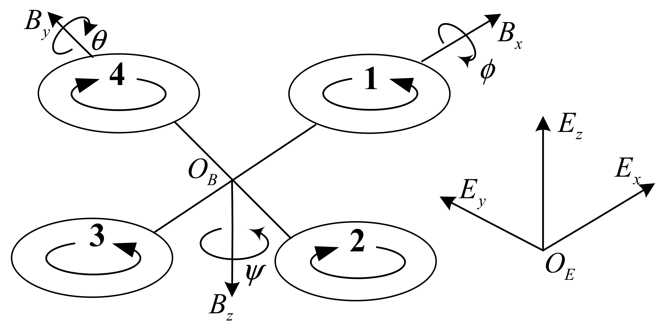
2.1. Dynamic Model of the Quadrotor

The UAV structure considered in this article is identical to that shown in Figure 1. For the ith quadrotor, the dynamic model considering disturbance and uncertainty can be obtained by the Lagrange method [37]:
ϕ ¨ i = a 1 u i , 1 + b 1 θ ˙ i ψ ˙ i + b 2 Ω r θ ˙ i + Δ f 1 + d 1 θ ¨ i = a 2 u i , 2 + b 3 ψ ˙ i ϕ ˙ i b 4 Ω r ϕ ˙ i + Δ f 2 + d 2 ψ ¨ i = a 3 u i , 3 + b 5 ϕ ˙ i θ ˙ i + Δ f 3 + d 3 x ¨ i = u i , x / m + Δ f 4 + d 4 y ¨ i = u i , y / m + Δ f 5 + d 5 z ¨ i = u i , z / m + Δ f 6 + d 6
where ( x i , y i , z i ) are the states of position; ( θ i , ϕ i , ψ i ) are pitch, roll, and yaw angle, respectively; m is the mass of the UAV; u i , x , u i , y , u i , z , and u i , j j = 1 , 2 , 3 are variables with control inputs; Ω r is the residual angular speed of the propellers; f i , d i j = 1 , , 6 are uncertainty and unknown disturbance, respectively; and d i d ¯ , in which d ¯ is a bounded positive number. The expressions of a j ( j = 1 , 2 , 3 ) and b k ( k = 1 , 2 , 3 , 4 , 5 ) can be found in [37]. u i , x , u i , y , and u i , z are as follows:
u i , x = u i , 4 cos ϕ i sin θ i cos ψ i + sin ϕ i sin ψ i u i , y = u i , 4 cos ϕ i sin θ i sin ψ i sin ϕ i cos ψ i u i , z = m g u i , 4 cos ϕ i cos θ i
where u i , 4 is the input of the translational subsystem and g is the acceleration of gravity.

2.2. Linear Discrete-Time Model of UAV

To facilitate the design of the MPC, the dynamic model of the quadrotor is divided into a rotational subsystem (RS) and translational subsystem (TS), and then linearized and discretized. For the RS, considering the disturbance, the linear time-varying discrete state-space model is as follows:
X i , R ( k + 1 ) = A i , R X i , R ( k ) + B i , R U i , R ( k ) + G D , R D i , R ( k ) Y i , R ( k + 1 ) = C i , R X ( k + 1 )
where X i , R ( k ) = ϕ i ( k ) ; ϕ ˙ i ( k ) ; θ i ( k ) ; θ ˙ i ( k ) ; ψ i ( k ) ; ψ ˙ i ( k ) is the state vector of the RS, U i , R ( k ) = u i , 2 ; u i , 3 ; u i , 4 ; Ω i , r is the input vector, and D i , R ( k ) = 0 ; d ^ i , R , 1 ( k ) ; 0 ; d ^ i , R , 2 ( k ) ; 0 ; d ^ i , R , 3 ( k ) is the synthesis of disturbance and uncertainty, where d ^ i , R , j ( k ) = Δ f j + d j , j = 1 , 2 , 3 . When the sampling period of the RS is T R , A i , R ,   B i , R ,   G D , R , and C i , R in (4) are:
A i , R = 1 T R 0 0 0 0 0 1 0 b 1 T R ψ ˙ i 0 b 1 T R θ ˙ i 0 0 1 T R 0 0 0 b 3 T R ψ ˙ i 0 1 0 b 3 T R ϕ ˙ i 0 0 0 0 1 T R 0 b 5 T R θ ˙ i 0 b 5 T R ϕ ˙ i 0 1 , B i , R = 0 0 0 0 T R a 1 0 0 T R b 2 θ ˙ i 0 0 0 0 0 T R a 2 0 T R b 4 θ ˙ i 0 0 0 0 0 0 T R a 3 0 G D , R = 0 0 0 0 0 0 0 T R 0 0 0 0 0 0 0 0 0 0 0 0 0 T R 0 0 0 0 0 0 0 0 0 0 0 0 0 T R , C i , R = 1 0 0 0 0 0 0 1 0 0 0 0 0 0 1 0 0 0 0 0 0 0 1 0
Similarly, the linear discrete-time model of TS is as follows:
X i , T ( k + 1 ) = A i , T X i , T ( k ) + B i , T U i , T ( k ) + G D , T D i , T ( k ) Y i , T ( k + 1 ) = C i , T X i , T ( k + 1 )
where X i , T ( k ) = x i ( k ) ; x ˙ i ( k ) ; y i ( k ) ; y ˙ i ( k ) ; z i ( k ) ; z ˙ i ( k ) is the state vector of the TS, U i , T ( k ) = u i , x ; u i , y ; u i , z is the input vector, and D i , T = 0 ; d ^ i , T , 4 ( k ) ; 0 ; d ^ i , T , 5 ( k ) ; 0 ; d ^ i , T , 6 ( k ) is the synthesis of disturbance and uncertainty, where d ^ i , T , j ( k ) = Δ f j + d j , j = 4 , 5 , 6 . When the sampling period of the TS is T T , A i , T ,   B i , T ,   G D , T , and C i , T in (6) are:
A i , T = 1 T T 0 0 0 0 0 1 0 0 0 0 0 0 1 T T 0 0 0 0 0 1 0 0 0 0 0 0 1 T T 0 0 0 0 0 1 , B i , T = 0 0 0 T T / m 0 0 0 0 0 0 T T / m 0 0 0 0 0 0 T T / m G D , T = 0 0 0 0 0 0 0 T T 0 0 0 0 0 0 0 0 0 0 0 0 0 T T 0 0 0 0 0 0 0 0 0 0 0 0 0 T T , C i , T = 1 0 0 0 0 0 0 0 1 0 0 0 0 0 0 0 1 0

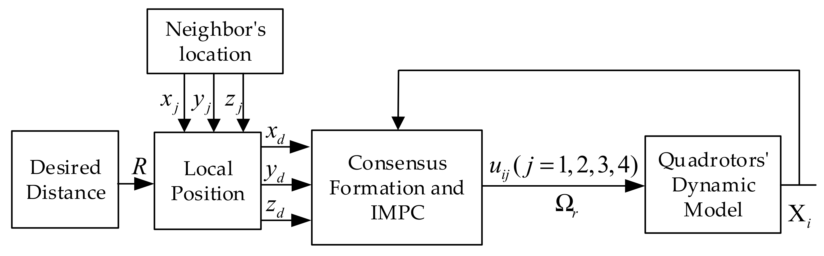
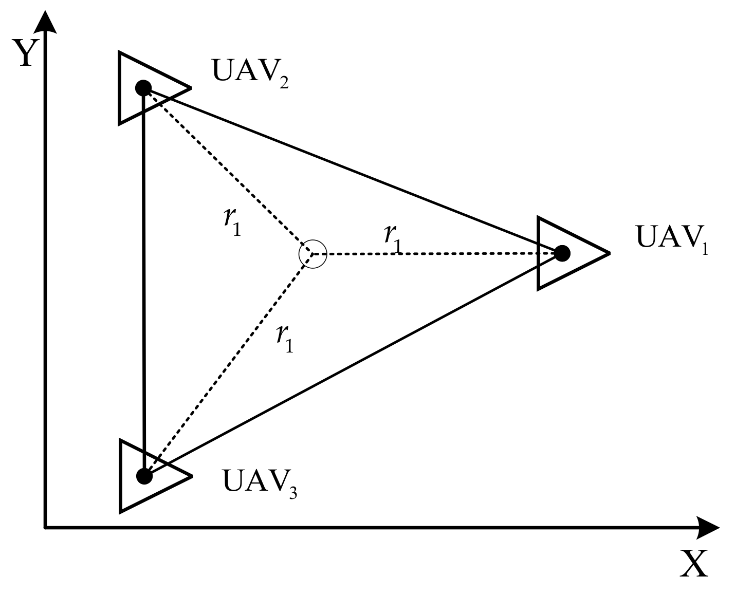
2.3. Formation Algorithm Based on Consensus

Since this paper focuses on the improvement of control performance as well as trajectory tracking capability, communication loss is not considered and it is assumed that all states of the UAVs can be shared among each other. Only the consensus of the position is considered here.
The undirected graph composed of n UAVs is given as Λ = { Δ , ε } , where Δ = { Δ 1 , Δ 2 , , Δ n } is the set of quadrotors; ε Δ × Δ is the edge of the graph, which means the states can be obtained between UAVs; and e i j indicates the weight of the edge between Δ i and Δ j . e i j = 1 if Δ i and Δ j can receive information from each other; otherwise, e i j = 0 . Take the x-axis of TS as an example:
x ˙ = x ˙ x ¨ = u i , x / m
The consensus law for the fixed topology of the formation on the x-axis is [7]:
u i , x , c ( t ) = j = 1 n e i j [ k x ( x i ( t ) x j ( t ) p i j ) ] , i = 1 , , n
where u i , x , c ( t ) is the component of consensus control low on the x-axis, p i j is the distance between UAV i and UAV j , and k x is the control coefficient that meets k x > 0 . The consensus laws u i , y , c ( t ) , u i , z , c ( t ) of the y- and z-axis, respectively, can be obtained in the same way.
The structure of the formation controller is shown in Figure 2. The stability and accuracy of the formation trajectory tracking are determined by both the consensus control law and IMPC.

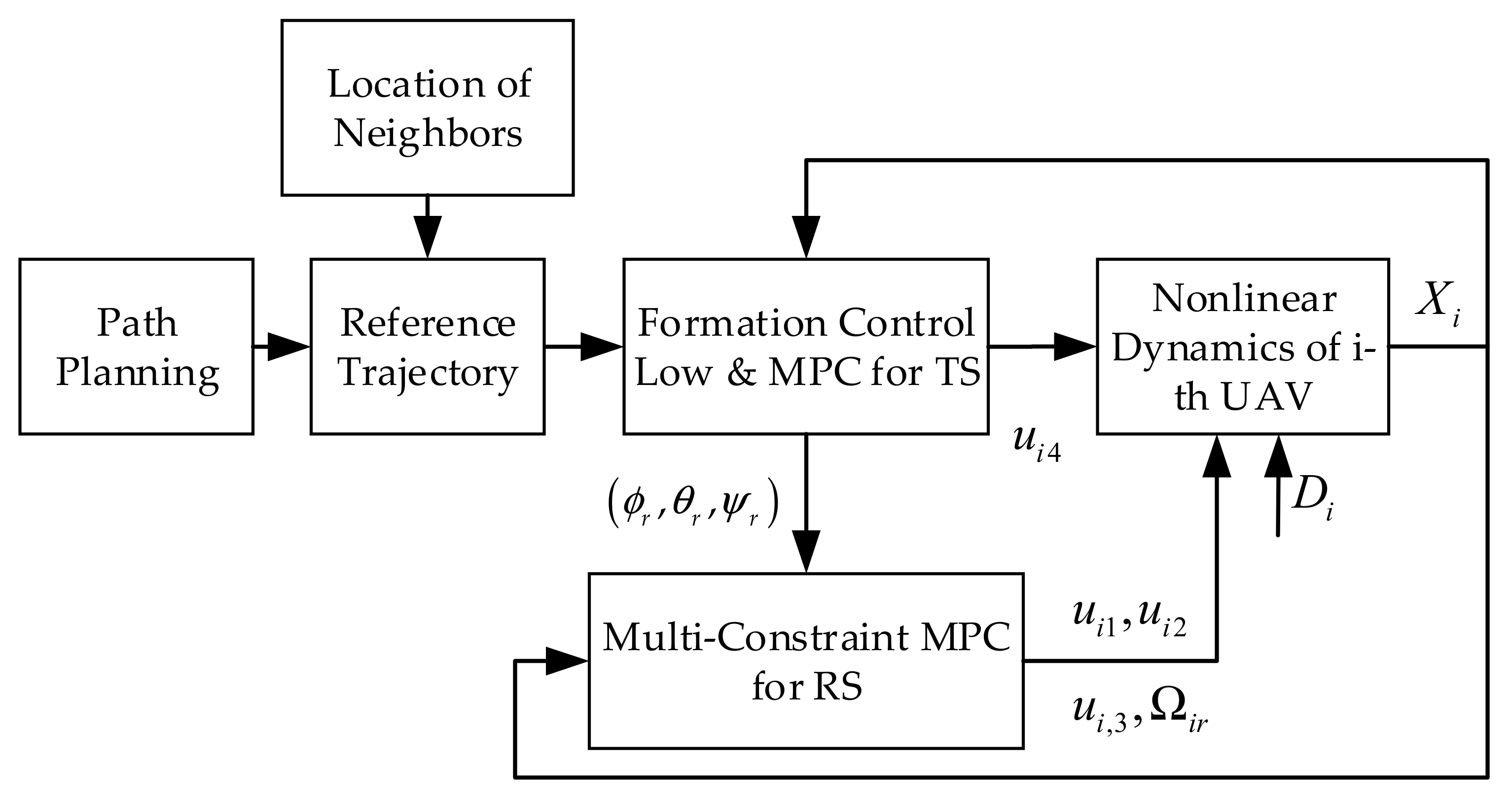
3. Multi-Constrained MPC

The multi-UAV system is a complex system with multiple constraints. MPC is one of the most effective methods to solve constrained control problems. Figure 3 illustrates the MPC structure of the ith quadrotor, where the planned path and the location of the neighbors determine the reference trajectory of the TS. The reference angle is generated by the TS and passed to the RS to stabilize the quadrotor.

3.1. MPC of TS

As shown in Figure 3, the controller of the TS is independent of the RS, while the results of the TS can provide reference values for the RS. Therefore, the MPC of the TS is implemented first. The difference equation of (5) is:
X i , T k + 1 X i , T k = A i , T X i , T k X i , T k 1 + B i , T U i , T ( k ) U i , T ( k 1 )     + G i , D , T D i , T ( k ) D i , T ( k 1 )
The augmented system is derived as follows:
X ^ i , T k + 1 = A ^ i , T X ^ i , T k + B ^ i , T U i , T ( k ) U i , T ( k 1 ) + G ^ i , D , T e D ( k ) Y i , T k + 1 = C ^ i , T X ^ i , T k + 1
where X ^ i , T k + 1 = X i , T k + 1 X i , T k Y i , T k + 1 , A ^ i , T = A i , T 0 6 × 3 C i , T A i , T I 3 × 3 , B ^ i , T = B i , T C i , T B i , T , G ^ i , d , T = G i , d , T C i , T G i , d , T , and C ^ i , T = 0 3 × 6 I 3 × 3 . e D ( k ) = D i , T ( k ) D i , T ( k 1 ) is a set of integrated white noise. Since the expected values of states are used in the calculation of the MPC, e D ( k ) = 0 . Assuming that N c , T is the number of future controls and N p , T is the length of the prediction, the predicted output vector Y ^ i , T and future control vector Δ U ^ i , T at time k are as follows:
Y ^ i , T k = Y i , T k + 1 | k ; Y i , T k + 2 | k ; ; Y i , T k + N p , T | k Δ U ^ i , T ( k ) = Δ U i , T ( k ) ; Δ U i , T ( k + 1 ) ; ; Δ U i , T ( k + N c , T 1 )
The predictive equation for future outputs within one optimization window is, by substitution:
Y ^ i , T k = M i , T X ^ i , T k | k + N i , T Δ U ^ i , T ( k )
where M i , T and N i , T are represented as follows:
M i , T = C ^ i , T A ^ i , T C ^ i , T A ^ i , T 2 C ^ i , T A ^ i , T 3 C ^ i , T A ^ i , T N p , T N i , T = C ^ i , T B ^ i , T 0 0 0 C ^ i , T A ^ i , T B ^ i , T C ^ i , T B ^ i , T 0 0 C ^ i , T A ^ i , T 2 B ^ i , T C ^ i , T A ^ i , T B ^ i , T C ^ i , T B ^ i , T 0 C ^ i , T A ^ i , T N p , T 1 B ^ i , T C ^ i , T A ^ i , T N p , T 2 B ^ i , T C ^ i , T A ^ i , T N p , T 3 B ^ i , T C ^ i , T A ^ i , T N p , T N c , T B ^ i , T
The essence of the constrained MPC is to minimize J i , T ( k ) at each sample k by solving the optimal control vector Δ U ^ i , T , and this minimization is based on the real-time optimization of J i , T ( k ) constrained by a series of linear inequalities. For UAV i , if the expected states at time k are r s ( k k ) = x r ( k k ) ; x ˙ r ( k k ) ; y r ( k k ) ; y ˙ r ( k k ) ; z r ( k k ) ; z ˙ r ( k k ) , the state vector-matrix for the new augmented system is rewritten as X ¯ i , T ( k + i | k ) = Δ X i , T ( k + i | k ) ; Y ( k + i | k ) C i , T r s ( k k ) . J i , T ( k ) and the linear inequality constraints are as follows:
min Δ U i , T J i , T k = i = 1 N p , T X ¯ i , T k + i | k T Q ¯ i , T X ¯ i , T k + i | k + j = 0 N c , T 1 Δ U i , T ( k + j ) T R ¯ i , T Δ U i , T ( k + j )       subject   to :   Γ i , T Δ U i , T ( k ) Θ i , T
where Q ¯ i , T = C ^ i , T T Q ^ i , T C ^ i , T , Q ^ i , T > 0 , and R ¯ i , T 0 . Γ i , T and Θ i , T represent the matrices when the constraints are converted to Δ U i , T [31].
The optimality and feasibility of this optimization problem is evaluated by the Kuhn–Tucker conditions of (14), which are satisfied. In order to minimize the cost function subject to constraints, the Lagrange form is obtained as:
min Δ U ^ i , T , λ i , T L i , T Δ U ^ i , T , λ i , T = R s , T Y ¯ i , T T Q i , T R s , T Y ¯ i , T + Δ U ^ i , T T R i , T Δ U ^ i , T + λ i , T T Γ i , T Δ U ^ i , T Θ i , T
where R s , T k k = C ^ i , T r ^ s k + 1 k ; C ^ i , T r ^ s k + 2 k ; ; C ^ i , T r ^ s k + N p k is the expected outputs matrix and r ^ s k + 1 k = 0 6 × 1 ; C i , T r s k + 1 k . Y ¯ i , T k = M i , T X ¯ i , T k k + N i , T Δ U ^ i , T ( k ) . Q i , T and R i , T are block diagonal matrices composed by Q ¯ i , T and R ¯ i , T , respectively. To decrease the computational burden of the constrained optimization problem, the active set methods (ASM) are applied in this paper. The specific process involves finding the inactive constraints and removing them at each moment of the rolling optimization process; only the active constraints are involved in the computational process of optimization [25]. Without losing generality, we assume that the desired output in one prediction window is slowly changing. By substituting Y ¯ i , T k into (15), the problem is equivalent to:
min Δ U ^ i , T , λ i , T L i , T Δ U ^ i , T , λ i , T = Δ U ^ i , T T N i , T T Q i , T N i , T + R i , T Δ U ^ i , T + 2 Δ U ^ i , T N i , T T Q i , T M i , T X ¯ i , T k k R s , T + λ i , T T Γ i , T Δ U ^ i , T Θ i , T
By taking derivatives of (16) with respect to Δ U ^ i , T and λ i , T , the optimal control vector and Lagrange multiplier of UAV i are obtained as follows:
Δ U ^ i , T k = ( N i , T T Q i , T N i , T + R i , T ) 1 N i , T T Q i , T M i , T X ¯ i , T k k R s , T k k + Γ i , T T λ i , T k 2         λ i , T k = 2 Γ i , T N i , T T Q i , T N i , T + R i , T 1 Γ i , T T 1 Θ i , T + Γ i , T N i , T T Q i , T N i , T + R i , T 1 N i , T T Q i , T M i , T X ¯ i , T k k R s , T k k
where λ i , T k 0 can be calculated using Hildreth’s quadratic programming procedure for each sample k. For each component of λ i , T k , if the Lagrange multiplier is positive, the corresponding component of Δ U ^ i , T k is a locally optimal point. For a negative Lagrange multiplier, the corresponding constraint can be omitted; that is, the corresponding component of λ i , T k is set to zero. Then Δ U ^ i , T k + 1 and λ i , T k + 1 can be obtained by continuous computation in the next step.
Remark 1. 
After solving the optimal problem, only the first row of  Δ U ^ i , T  is used, and the control signal for the next optimization window is  u i , x , m ( k + 1 ) ; u i , y , m ( k + 1 ) ;   u i , z , m ( k + 1 ) = U i , T k + Δ U ^ i , T , while the control law considering consensus and the MPC is  u i , x ( k + 1 ) ; u i , y ( k + 1 ) ; u i , z ( k + 1 ) = u i , x , m ( k + 1 ) ; u i , y , m ( k + 1 ) ; u i , z , m ( k + 1 ) + u i , x , c ( k + 1 ) ; u i , y , c ( k + 1 ) ; u i , z , c ( k + 1 ) . Supposing that the reference yaw angle is zero, the control signal of the  UAV i s TS at time  k + 1  is:
u i , 4 ( k + 1 ) = ( u i , z ( k + 1 ) m g ) 2 + u i , x 2 ( k + 1 ) + u i , y 2 ( k + 1 )
Assuming that π / 2 < ϕ i , r , θ i , r < π / 2 , the reference angles ϕ i , r and θ i , r can be calculated as:
ϕ i , r ( k + 1 ) = arcsin u i , y ( k + 1 ) u i , 4 ( k + 1 ) θ i , r ( k + 1 ) = arcsin u i , x ( k + 1 ) u i , 4 ( k + 1 ) cos ( ϕ i , r ( k + 1 ) )
Finally, the reference states for the RS at time k will be:
ϕ i , r ( k + 1 ) ; ϕ i , r ( k + 1 ) ϕ i , r ( k ) T T ; θ i , r ; θ i , r ( k + 1 ) θ i , r ( k ) T T ; 0 ; 0

3.2. MPC of the Rotational Subsystem

Similar to the TS, the optimal control and Lagrange multiplier of the RS are obtained as follows:
Δ U ^ i , R k + 1 = ( N i , R T Q i , R N i , R + R i , R ) 1 N i , R T Q i , R           M i , R X ¯ i , R k k R s , R k k + Γ i , R T λ i , R k + 1 2         λ i , R k + 1 = 2 Γ i , R N i , R T Q i , R N i , R + R i , R 1 Γ i , R T 1 Θ i , R   + Γ i , R N i , R T Q i , R N i , R + R i , R 1 N i , R T Q i , R M i , R X ¯ i , R k k R s , R k k
Therefore, after solving the above optimization problems, the first row of Δ U ^ i , R is selected as the incremental control signal of the RS and applied to UAV i .

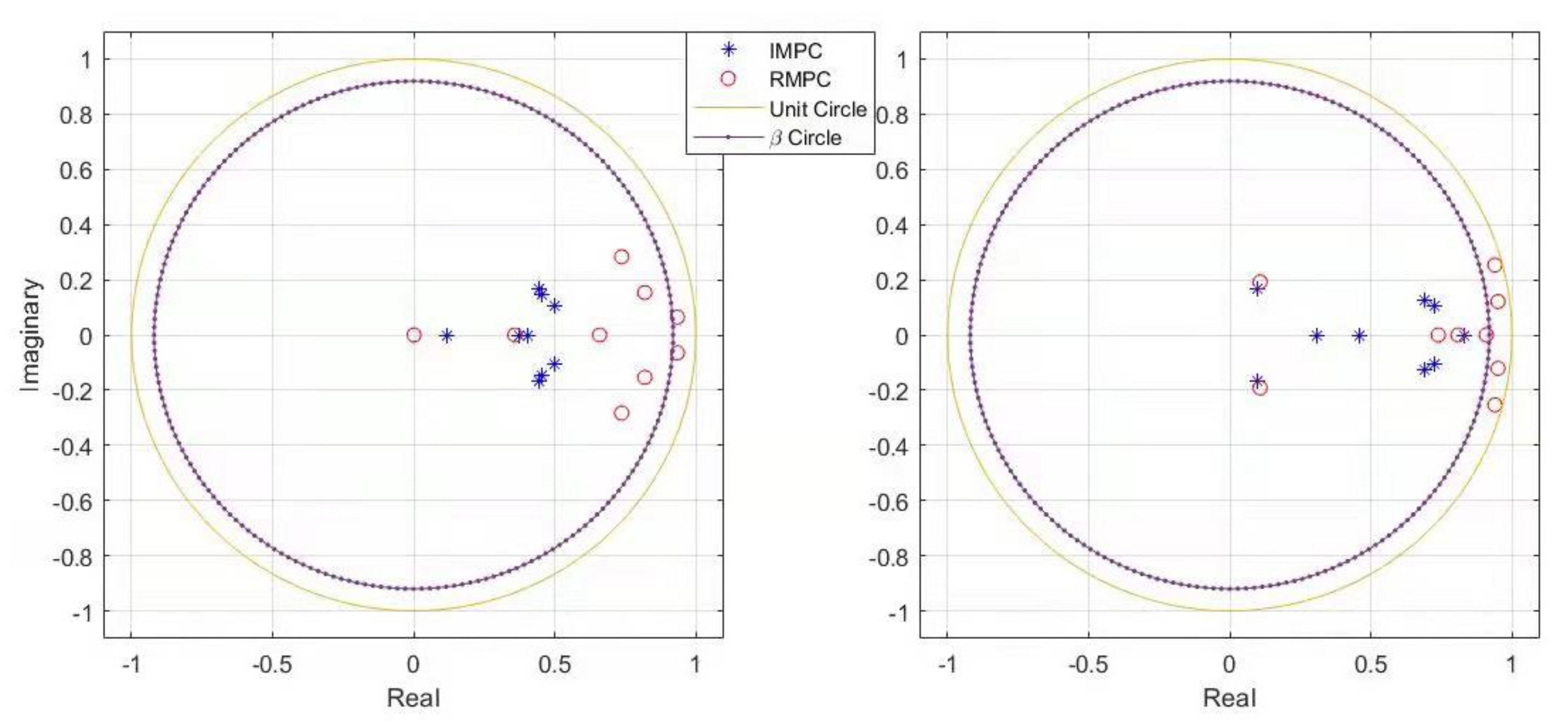
4. Stability Analysis
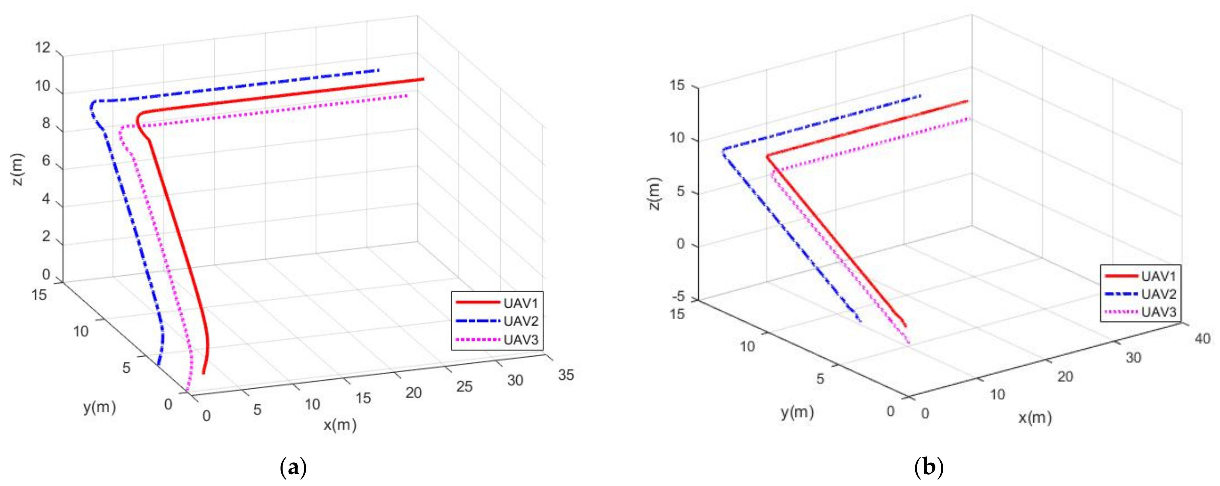
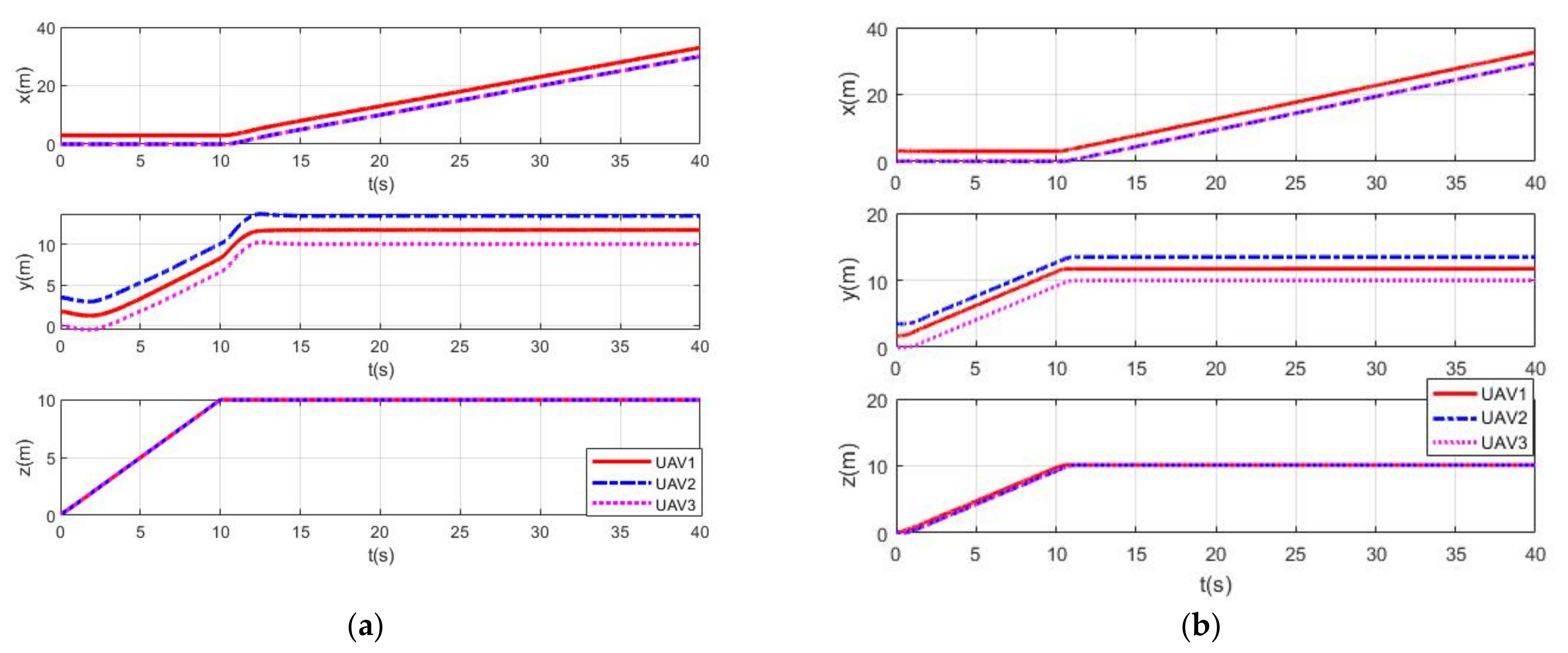
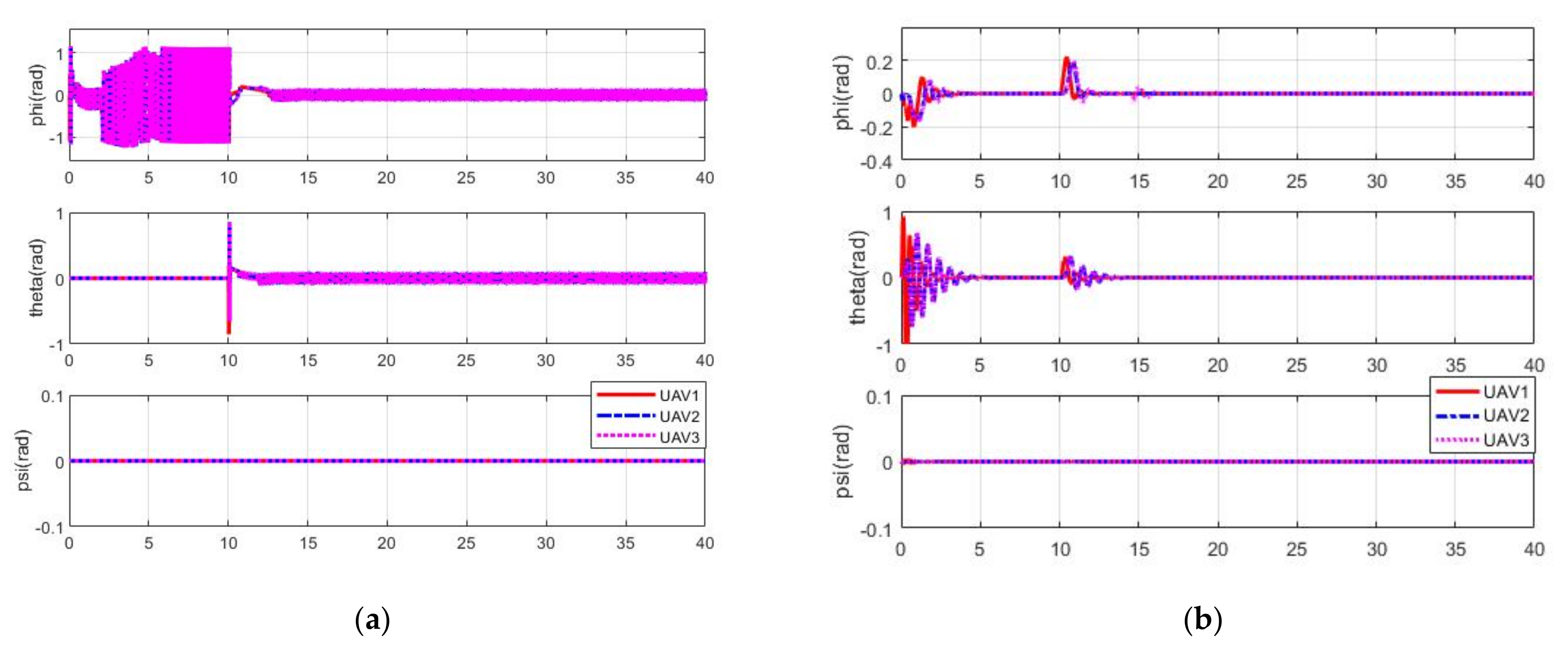
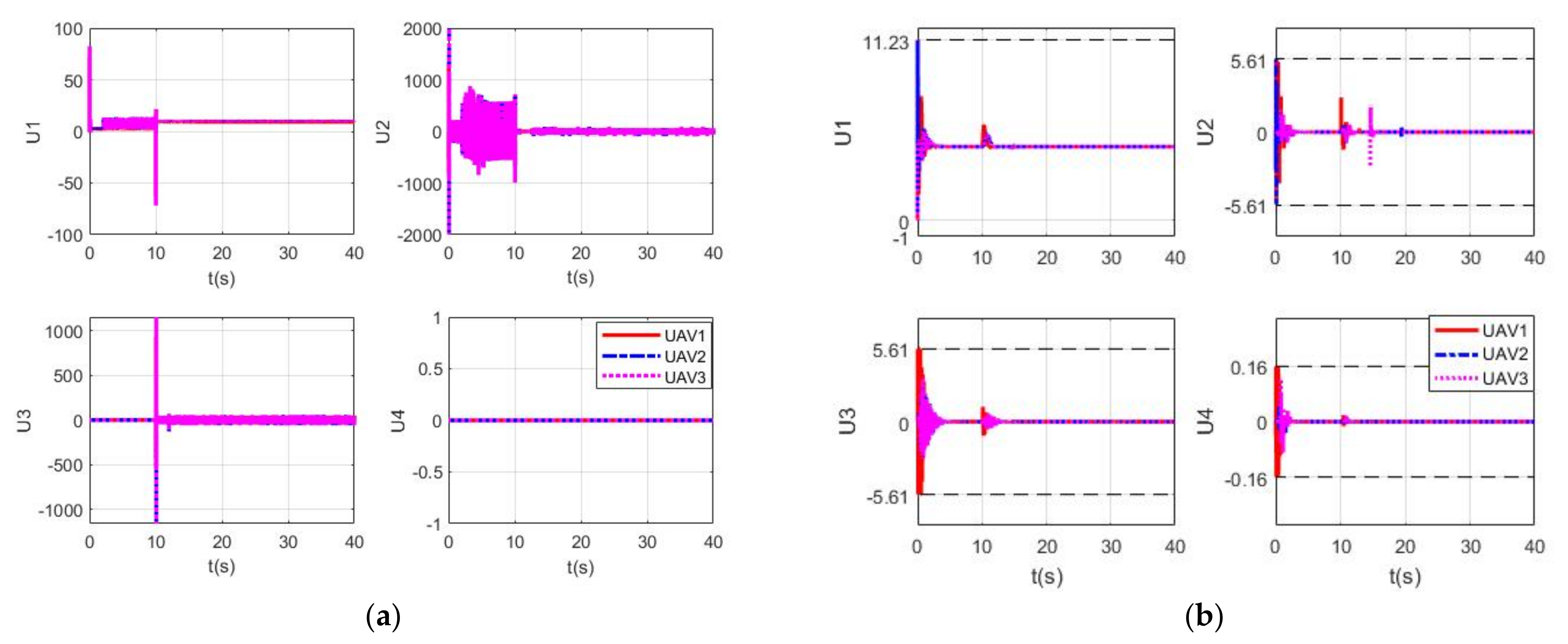
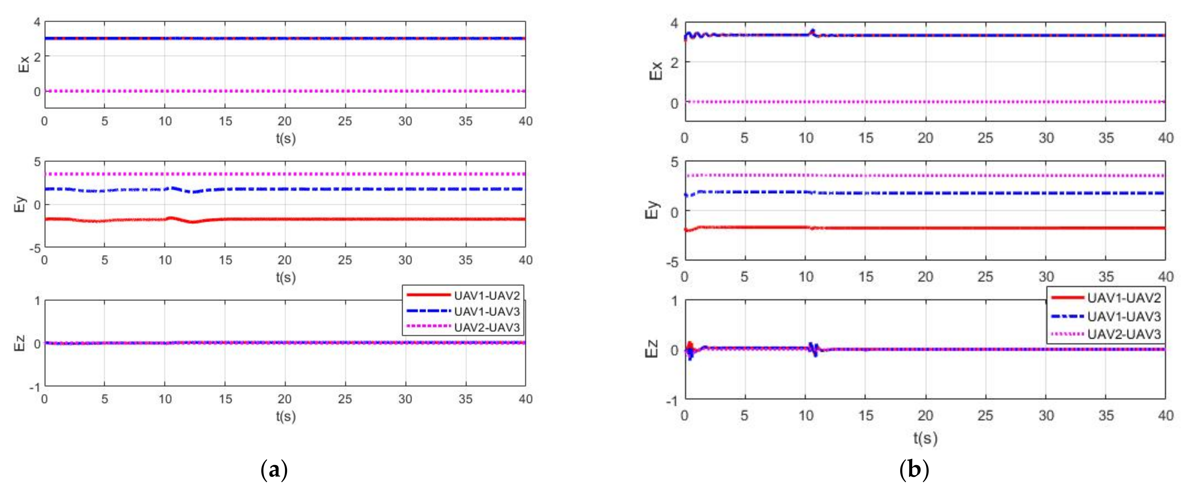
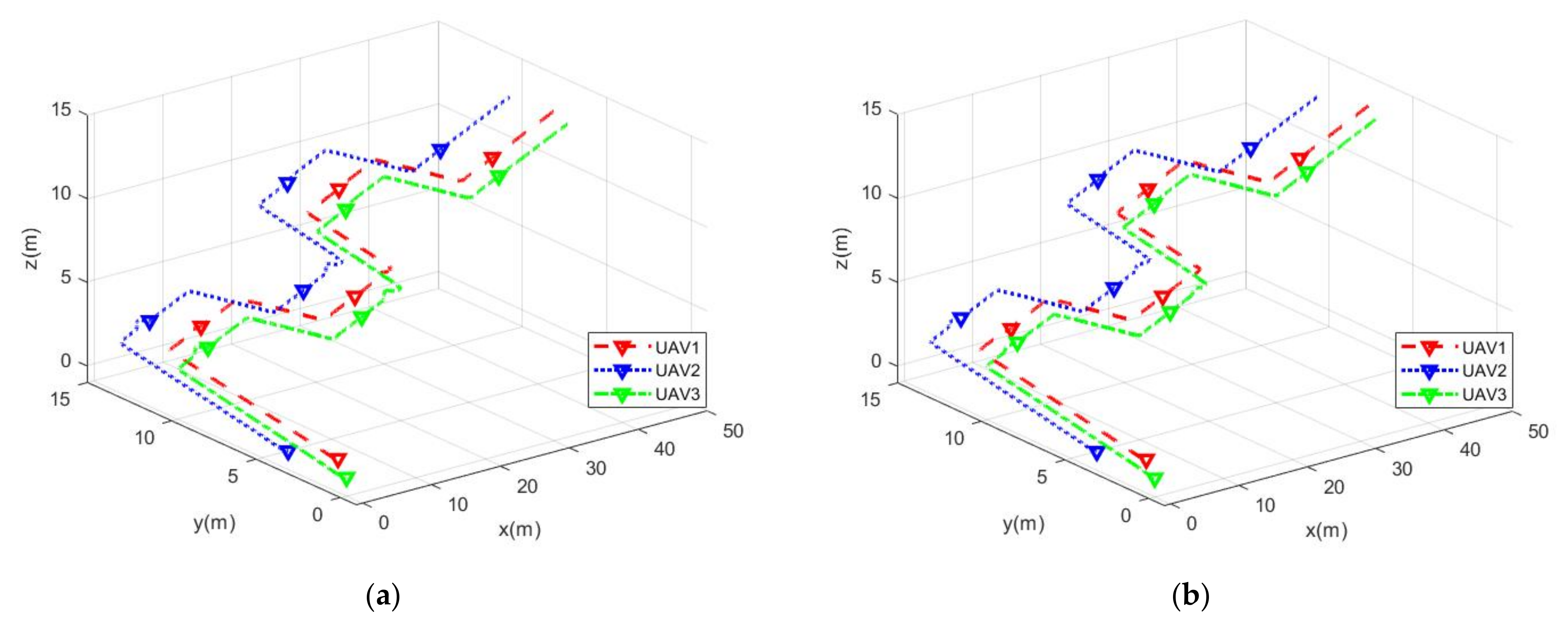
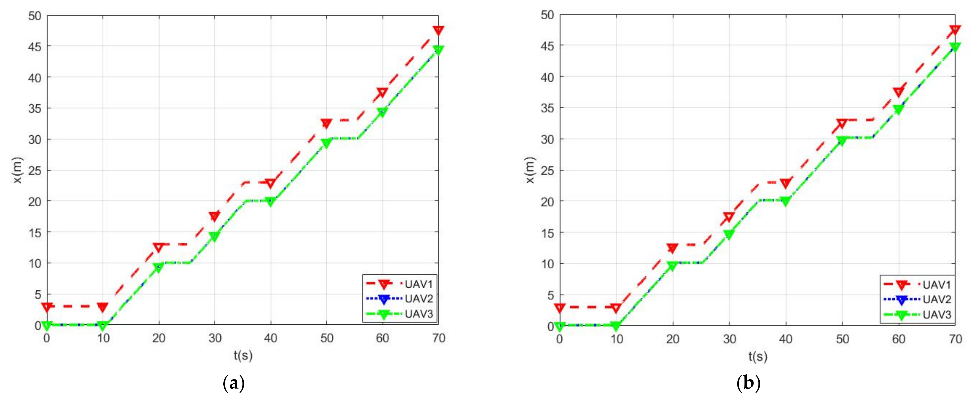
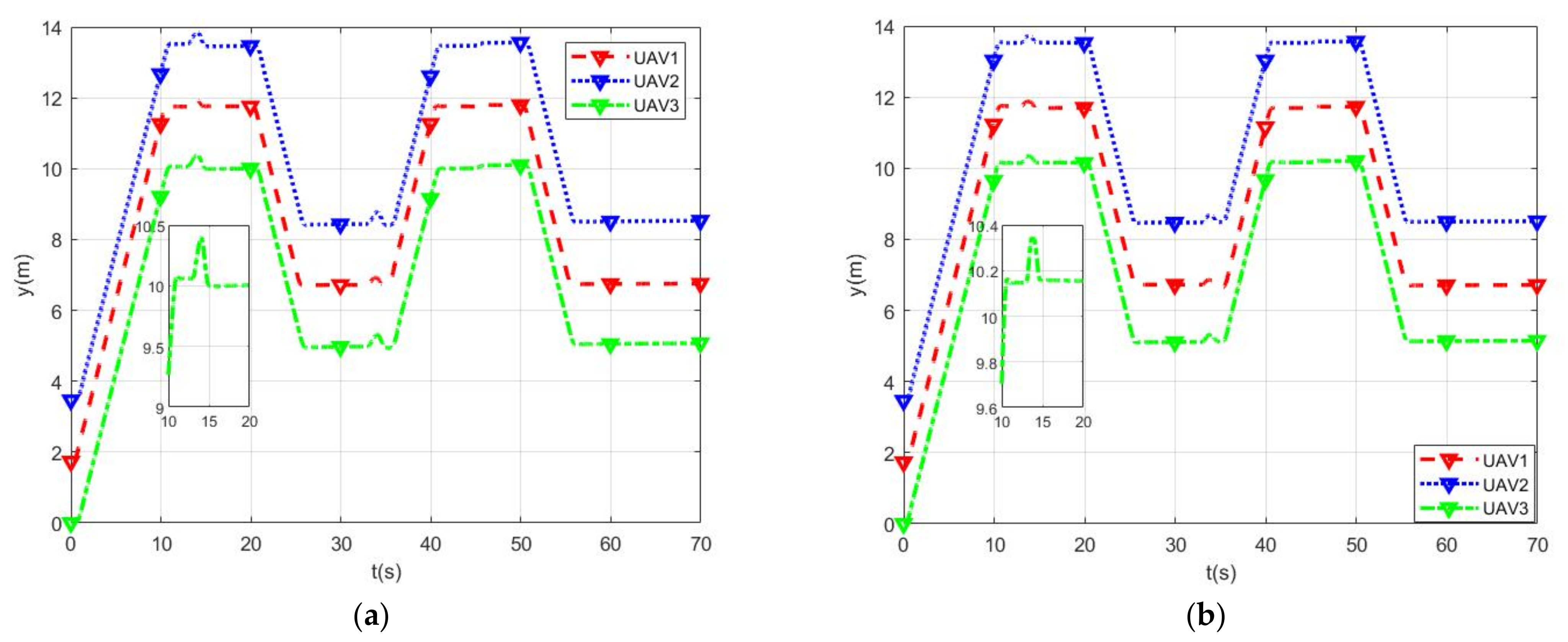
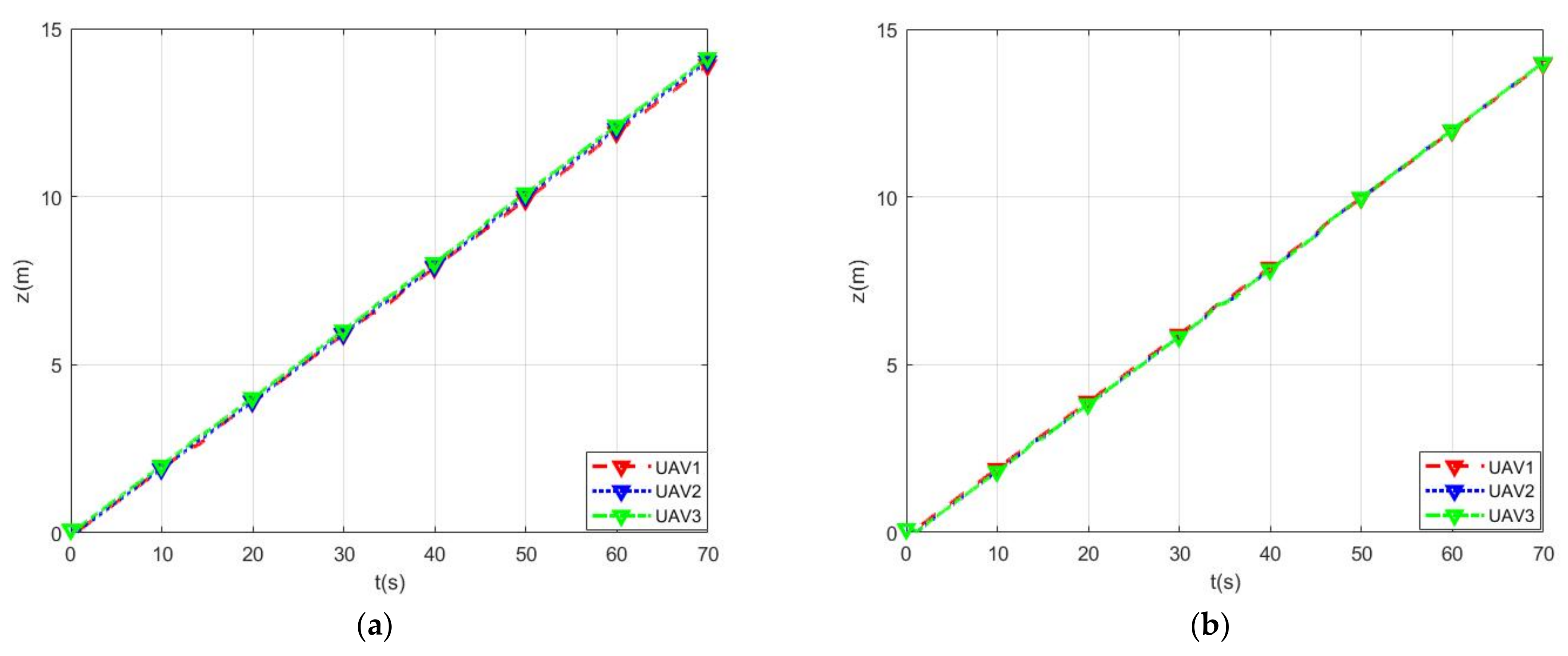
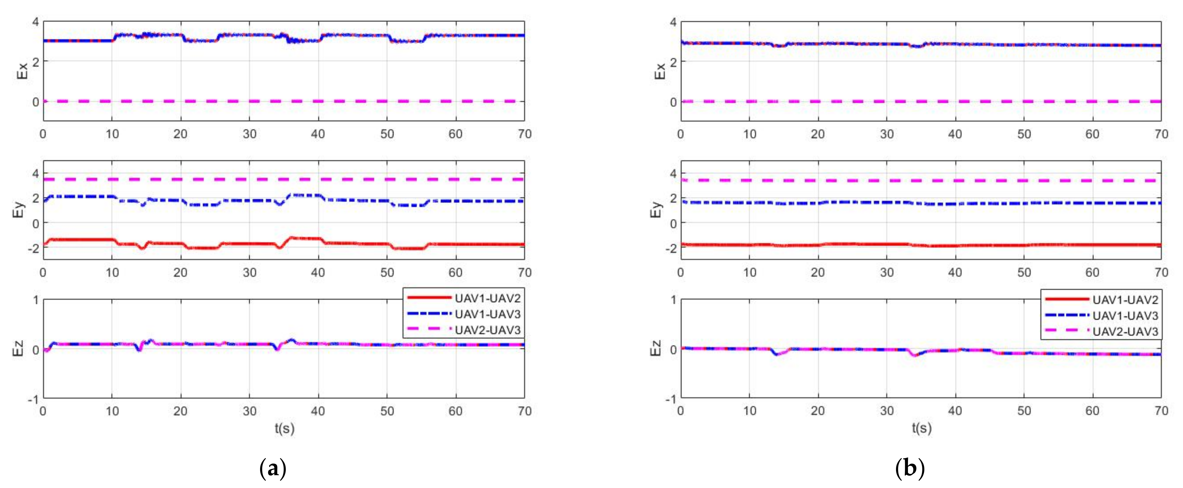
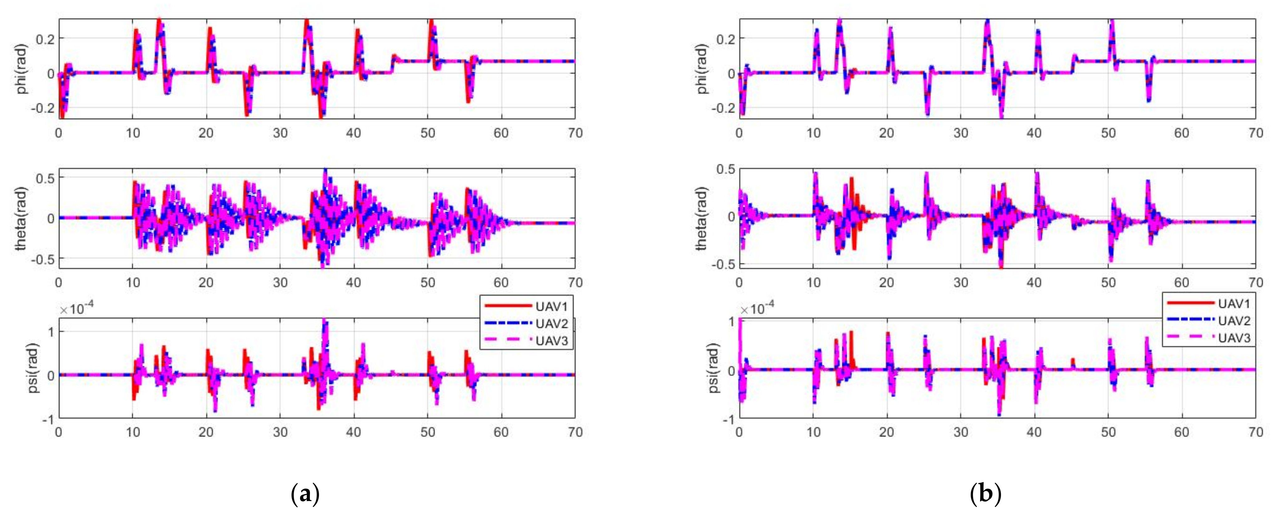
Since the integrators were introduced in the augmentation system, the condition number in (17) and (21) deteriorates if N P , T is large [32]. As can be seen from (4) and (6), the eigenvalues are in the vicinity of the unit circle, which will make the numerical problem worse. Therefore, it is necessary to make sure that the controller can avoid the drawback while ensuring the stability of the closed-loop system. Similar to the introduction of exponential factors in the linear quadratic regulator (LQR), the same modification can be made in MPC, which will push the poles of the closed-loop system into the unit circle. The benefits can be obtained through the following analysis.
For the convenience of analysis, the expected outputs are ignored without affecting the results. Take the TS as an example (the analysis of the RS is the same), with a given τ T > 1 , the cost function J i , T k with exponential factors in MPC can be processed as follows:
min Δ U i , T J i , T k = m = 1 N p , T τ T 2 m X ^ i , T k + m | k T Q ¯ i , T X ^ i , T k + m | k + j = 0 N c , T 1 τ T 2 j Δ U i , T ( k + j ) T R ¯ i , T Δ U i , T ( k + j )     subject   to : Γ i , T Δ U i , T ( k ) Θ i , T
where τ T > 1 means that the cost function J i , T k places more emphasis on the states and control of the current time than the states of the future; the weights decrease as m and j increase. Thus, the sequence of new states and incremental control vectors in one prediction window are chosen as follows:
X ^ τ k = τ T 1 X ^ i , T k + 1 | k T τ T 2 X ^ i , T k + 2 | k T τ T N p , T X ^ i , T k + N p , T | k T T Δ U ^ τ ( k ) = τ T 0 Δ U i , T ( k | k ) T τ T 1 Δ U i , T ( k + 1 | k ) T τ T ( N c , T 1 ) Δ U i , T ( k + N c , T 1 | k ) T T
where the elements of X ^ τ k and Δ U ^ τ ( k ) are:
X ^ τ k + m + 1 k = τ T m + 1 X ^ i , T k + m + 1 k Δ U ^ τ k + m k = τ T m Δ U i , T k + m k
As described in (5), the elements of X ^ τ k and Δ U ^ τ ( k ) satisfy the following difference equation:
X ^ τ k + m + 1 | k = A ^ i , T τ T X ^ τ k + m | k + B ^ i , T τ T Δ U ^ τ ( k + m )
The optimization problem with multiple constraints can be rephrased as:
min Δ U ^ τ J τ k = m = 1 N p , T X ^ τ k + m | k T Q ¯ i , T X ^ τ k + m | k   + j = 0 N c , T 1 Δ U ^ τ ( k + j ) T R ¯ i , T Δ U ^ τ ( k + j )   subject   to :   Γ T , τ Δ U ^ τ ( k ) Θ T , τ
where Γ T , τ is as follows:
Γ T , τ = Γ T I 0 0 0 τ T I 0 0 0 τ T N p , T I
As can be seen from (14) and (26), the two cost functions have the same form and are identical to each other. Moreover, the optimal solution of (26) is Δ U ^ τ k + 0 k = τ T 0 Δ U i , T k k = Δ U i , T k k , which is the same as the answer to (14). Therefore, if τ T > 1 is chosen properly, the cost function (26) could be used in the process of MPC, while all the eigenvalues of τ T 1 A ^ i , T are inside the unit circle. The corresponding state space (25) is stable, which has a positive effect on solving the numerical problems in the MPC calculation process even if N P , T is large. However, the optimization problem (25) is equivalent to the discrete-time linear quadratic regulator (DLQR) problem when N P , T and N C , T are large enough [34,35,36]. The DLQR problem of the corresponding state-space model τ T 1 A ^ i , T , τ T 1 B ^ i , T is always solved by the algebraic Riccati equation, as follows with the same weight matrices Q ¯ i , T and R ¯ i , T :
A ^ i , T T τ T S A ^ i , T τ T S A ^ i , T T τ T S B ^ i , T τ T B ^ i , T T τ T S B ^ i , T τ T + R ¯ i , T 1 B ^ i , T T τ T S A ^ i , T τ T + Q ¯ i , T = 0
The state feedback control gain matrix K T , τ and the corresponding closed-loop system can be obtained as follows:
K T , τ = ( τ T 2 B ^ i , T T S B ^ i , T + R ¯ i , T ) 1 τ T 2 B ^ i , T T S A ^ i , T X ^ τ ( k + m + 1 | k ) = τ T 1 ( A ^ i , T B ^ i , T K T , τ ) X ^ τ ( k + m | k )
Since τ T > 1 is chosen, the eigenvalue λ max τ T 1 ( A ^ i , T B ^ i , T K T , τ ) < 1 can be guaranteed, while the eigenvalue of the actual system will be λ max ( A ^ i , T B ^ i , T K T , τ ) < τ T , which means there is no guarantee of the actual closed-loop system’s stability. However, it can be solved by choosing the values of Q ¯ i , T and R ¯ i , T properly.
Theorem 1. 
Let  σ T = τ T 1 β T , 0 < β T < 1 , Q σ = σ T 2 Q ¯ i , T + ( 1 σ T 2 ) S , and R σ = σ T 2 R ¯ i , T . The optimal solution of (30) can ensure the stability of the closed-loop system by choosing a suitable  β T .
min Δ U ^ α J σ k = m = 1 N p , T X ^ τ k + m | k T Q σ X ^ τ k + m | k + j = 0 N c , T 1 Δ U ^ τ ( k + j ) T R σ Δ U ^ τ ( k + j ) subject   to : Γ T , τ Δ U ^ τ ( k ) Θ T , τ
Proof of Theorem 1.
Similar to (26) and (28), the algebraic Riccati equation of (30) is:
A ^ i , T T τ T S A ^ i , T τ T S A ^ i , T T τ T S B ^ i , T τ T B ^ i , T T τ T S B ^ i , T τ T + R σ 1 B ^ i , T T τ T S A ^ i , T τ T + Q σ = 0
Substituting Q σ and R σ into (31) gives:
A ^ i , T T τ T S A ^ i , T τ T S A ^ i , T T τ T S B ^ i , T τ T B ^ i , T T τ T S B ^ i , T τ T + β T 2 R ¯ i , T τ T 2 1 B ^ i , T T τ T S A ^ i , T τ T + β T 2 Q ¯ i , T τ T 2 + S β T 2 S τ T 2 = 0
Multiplying both sides of (32) by τ T 2 β T 2 results in the following equivalent equation:
A ^ i , T T β T S A ^ i , T β T A ^ i , T T β T S B ^ i , T β T B ^ i , T T β T S B ^ i , T β T + R ¯ i , T 1 B ^ i , T T β T S A ^ i , T β T + Q ¯ i , T S = 0
The corresponding states feedback gains matrix K T , σ and closed-loop system are obtained as follows:
K T , σ = R ¯ i , T + β T 2 B ^ i , T T S B ^ i , T 1 β T 2 B ^ i , T T S A ^ i , T X ^ τ ( k + m + 1 | k ) = β T 1 ( A ^ i , T B ^ i , T K T , σ ) X ^ τ ( k + m | k )
where the definition of X ^ τ ( k + m + 1 | k ) is the same as (29). From the closed-loop system equation in (34), it can be seen that an appropriate choice of β T < 1 can ensure the eigenvalue λ max ( A ^ i , T B ^ i , T K T , σ ) < β T , which means that the closed-loop system is stable. □
In summary, the IMPC proposed here can improve the stability margin of the system by forcing the poles of the closed-loop system into the unit circle. Therefore, IMPC is able to cope with the influence of disturbances and the uncertainties of the system itself. Compared with RMPC, IMPC has better dynamic performance, which enables the system to return to steady state faster. The focus is on the continuous transformation of the original cost function (14) by (22) and (30), which is equivalent to obtaining the final closed-loop function as shown in (34). As mentioned earlier, the purpose of this is not only to ensure the stability of the model used in the predictive control process, but also the closed-loop system. At the same time, N P , T and N C , T can be large without numerical problems.

5. Simulation

The tasks of trajectory tracking and instructions procurement can be completed by UAV 1 . The main parameters of the UAV can be obtained from [19].
The following two cases are presented in the simulation: (1) A comparison with the dual closed-loop sliding mode formation controller under ideal dynamics [19]. (2) A comparison of IMPC and RMPC in achieving the same formation trajectory tracking in the presence of disturbance and model uncertainty.

5.1. Case 1

The distance of the three axes between UAVs remained the same in this simulation. Figure 4 shows the geometry of three UAVs’ formation flights in Case 1, where r 1 = 2   m .
The expected trajectory in case 1 is as follows:
R x 1 = 3 ,   t 10   s   3 + t 10 , t > 10   s ,   R y 1 = 1.732 + t ,     t 10   s 11.732 ,     t > 10   s ,   R z 1 = 0.1 + t ,     t 10   s 10.1 ,     t > 10   s
where R x , R y , and R z are the expected trajectories of axis X, Y, Z, respectively.
The initial positions of the three UAVs were: UAV 1 (3, 1.732, 0.1) m, UAV 2 (0, 3.464, 0.1) m, and UAV 3 (0, 0, 0.1) m. The initial speeds were all 0 m/s. For the TS, the sampling period was T S = 0.05   s , while T R = 0.05   s for the RS. The main parameters of IMPC in the rolling optimization process were: Q ^ i , T = Q ^ i , R = 20 , R ¯ i , T = R ¯ i , R = 0.01 I 6 , where I 6 was the unit matrix; N c , T = N c , R = 1 ; N p , T = 10 ; N p , R = 4 , τ T = 1.6 ; β T = 0.92 ; τ R = 1.2 ; and β R = 0.92 . The parameters of the consensus low were k x = k y = k z = 0.01 . Due to the constraints of UAVs’ rotor, the states and inputs were limited as follows:
π 2 ( rad ) < ϕ , θ < π 2 ( rad ) ,   0 < ψ < π ( rad ) ,   0.76 ( rad s 1 ) < ϕ ˙ , θ ˙ < 0.76 ( rad s 1 )
1 ( rad s 1 ) < ψ ˙ < 1 ( rad s 1 ) ,   1.5 ( m s 1 ) x ˙ ,   y ˙ ,   z ˙ 1.5 ( m s 1 )
0 U 1 11.23 ( N ) ,   | U 2 | 5.61 ( N m ) ,   | U 3 | 5.61 ( N m ) ,   | U 4 | 0.16 ( N m )
The simulation results are shown in Figure 5, Figure 6, Figure 7, Figure 8 and Figure 9. The total time of simulation was 40 s. Figure 5 shows the trajectory tracking of the UAVs in 3D space with SMC (a) and IMPC (b). Figure 6 and Figure 7 illustrate the states of the TS and RS, respectively, demonstrating that the UAVs with IMPC (b) provide significantly better performance than SMC (a). Figure 8 and Figure 9 exhibit the inputs and distance of the three axes of the formation, respectively. They show that in order to maintain the expected formation, the inputs of SMC (a) must been far greater, while IMPC (b) can remain within the specified constraints. The reason for the oscillation process of SMC in Figure 7, Figure 8 and Figure 9 is the fact that the large uncertainty in the model requires a large gain of the switching term, which can be solved by replacing the symbolic function with a saturation function [38].

5.2. Case 2

For Case 2, the formation structure and main parameters of IMPC were the same as in Case 1. The expected trajectory in this part was:
R x 2 = 3 ,   t 10   s 3 + ( t 10 ) ,   10   s < t 20   s   13 ,   20   s < t 25   s 13 + ( t 25 ) ,   25   s < t 3 5   s 23 ,   35   s < t 40   s   23 + ( t 40 ) ,   40   s < t 50   s   33 ,   50   s < t 55   s 33 + ( t 55 ) ,   25   s < t 3 5   s ,   R y 2 = 1.732 + t ,   t 10   s 11 . 732 ,   10   s < t 20   s 11.732 ( t 20 ) ,   20   s < t 25   s 6.732 ,   25   s < t 35   s 6.732 + ( t 35 ) ,   35   s < t 40   s   11 . 732 ,   40   s < t 50   s 11.732 ( t 50 ) ,   50   s < t 55   s 6.732 ,   t > 55   s ,   R z 2 = 0.2 t
The initial positions of the three UAVs were: UAV 1 (3, 1.732, 0.1) m, UAV 2 (0.1, 3.464, 0.1) m, and UAV 3 (0.1, 0.1, 0.1) m. In the real formation flight, the quantified uncertainties and disturbances were unknown and had to be estimated online. To verify the robustness of IMPC to the uncertainties and disturbances, they were simply set to fixed values. The synthesis of uncertainties and disturbances of the UAV i in the formation given in this paper are d i , 1 = 0.4 , d i , 2 = 0.1 , d i , 3 = 0.1 , d i , 4 = 0.3 , d i , 5 = 0.3 and d i , 6 = 0.1 , while the additional impulse for the TS given in this paper is I M i , 1 , where:
I M i , 1 = [ 0 ; 3 ; 0 ; 3 ; 0 ; 1 ] ,   13   s < t 14   s ,   33   s < t 34   s [ 0 ; 0.7 ; 0 ; 0.7 ; 0 ; 0.1 ] ,   t > 45   s
The condition number of regular MPC (RMPC) and IMPC is shown in Table 1, where the TS of IMPC was about two orders of magnitude less than RMPC, and the RS of RMPC was about twice that of IMPC. This means that the computational complexity of the IMPC designed in this paper can be greatly reduced compared to the RMPC. The average computation period also demonstrates the superiority of IMPC.
The poles of the closed-loop system for the TS and RS lie in the circle of β T = β R = 0.92 with IMPC, as shown in Figure 10, which makes the closed-loop system more stable than RMPC.
The simulation results are shown in Figure 11, Figure 12, Figure 13, Figure 14, Figure 15 and Figure 16. Figure 11, Figure 12, Figure 13 and Figure 14 show the formation trajectory tracking in the presence of disturbances and uncertainties. As can be seen from the figure, both controllers were able to suppress the effects of disturbances and system uncertainties. However, the formation with IMPC (b) had smaller errors and a shorter settling time than that of RMPC (a). Figure 15 describes the distance between the UAVs on three axes, where IMPC (b) had better formation stability than RMPC (a). As can be seen in Figure 16, the angle of the UAVs in formation changed when they turned or were affected by disturbances; with IMPC, the changes in the angles were much smoother and took less time to return to the stable states. This is further supported by the control inputs in Figure 17.

6. Conclusions and Future Work

The formation control based on consensus and IMPC was proposed in this paper to ensure the stability and trajectory tracking of the formation. A literature investigation showed that most studies are based on simplified or ideal models, and constraints on UAVs are not paid enough attention.
Firstly, the UAV dynamic model with disturbance and uncertainty is introduced, and it is divided into an RS and a TS. The corresponding multi-constrained IMPC is designed after obtaining the error-augmented models of the two subsystems. The influence of external disturbance and uncertainty can be eliminated because of the integral in the augmented system. On this basis, by appropriately modifying the cost function, not only can the numerical problems in the rolling optimization process be reduced, but also the stability of the two closed-loop subsystems is ensured.
Because of the addition of integrators to the augmented model, it is possible to eliminate the effect of disturbances and model uncertainties on the performance of the controller without adding disturbance observers.
The simulation results demonstrate that the proposed procedure guarantees a better formation effect than SMC under the condition of hard constraints. The IMPC outperformed the RMPC in terms of condition number, which means that IMPC has higher computational efficiency. It can be seen from the final simulation that IMPC can eliminate the influence of disturbance and uncertainty. The robustness to impulse can provide a meaningful reference for pesticide spraying and other formation problems under load.
Future work should consider the challenges of parameter changes, obstacle avoidance, and reconstruction problems.

Author Contributions

D.Y. constructed the tracking framework, performed the experiments, and wrote the original manuscript. H.C. analyzed and interpreted the experimental results. W.Z. provided suggestions about the revision of this manuscript. All authors have read and agreed to the published version of the manuscript.

Funding

This work was supported by the National Natural Science Foundation of China (No. 62073266).

Acknowledgments

D.Y. would like to thank Xiang Gao for the support. The authors wish to thank the anonymous reviewers for their valuable suggestions.

Conflicts of Interest

The authors declare no conflict of interest.

References

  1. Josep, M.G.; Rogelio, L. Flight Formation Control; John Wiley & Sons: Hoboken, NJ, USA, 2012. [Google Scholar]
  2. Zong, Q.; Wang, D.; Shao, S.; Zhang, B.; Han, Y. Research status and development of multi UAV coordinated formation flight control. J. Harbin Inst. Technol. 2017, 49, 1–14. [Google Scholar]
  3. Fu, X.; Pan, J.; Wang, H.; Gao, X. A Formation Maintenance and Reconstruction Method of UAV Swarm based on Distributed Control. Aerosp. Sci. Technol. 2020, 104, 105981. [Google Scholar] [CrossRef]
  4. Liu, H.; Lyu, Y.; Zhao, W. Robust visual servoing formation tracking control for quadrotor UAV team. Aerosp. Sci. Technol. 2020, 106, 106061. [Google Scholar] [CrossRef]
  5. Zhen, Z.; Tao, G.; Xu, Y.; Song, G. Multivariable adaptive control based consensus flight control system for UAVs formation. Aerosp. Sci. Technol. 2019, 93, 105336. [Google Scholar] [CrossRef]
  6. Yu, Z.; Zhang, Y.; Jiang, B.; Su, C.Y.; Fu, J.; Jin, Y.; Chai, T. Decentralized fractional-order backstepping fault-tolerant control of multi-UAVs against actuator faults and wind effects. Aerosp. Sci. Technol. 2020, 104, 105939. [Google Scholar] [CrossRef]
  7. Wolfe, S.; Givigi, S.; Rabbath, C.A. Distributed Multiple Model MPC for Target Tracking UAVs. In Proceedings of the 2020 International Conference on Unmanned Aircraft Systems (ICUAS), Athens, Greece, 9–12 June 2020; IEEE: Piscataway, NJ, USA, 2020; pp. 123–130. [Google Scholar]
  8. Huang, H.; Zhou, H.; Zheng, M.; Xu, C.; Zhang, X.; Xiong, W. Cooperative Collision Avoidance Method for Multi-UAV Based on Kalman Filter and Model Predictive Control. In Proceedings of the 2019 IEEE International Conference on Unmanned Systems and Artificial Intelligence (ICUSAI), Xi’an, China, 22–24 November 2019; IEEE: Piscataway, NJ, USA, 2019; pp. 1–7. [Google Scholar]
  9. Kuriki, Y.; Namerikawa, T. Formation Control with Collision Avoidance for a Multi-UAV System Using Decentralized MPC and Consensus-Based Control. SICE J. Control Meas. Syst. Integr. 2015, 8, 285–294. [Google Scholar] [CrossRef]
  10. Chao, Z.; Zhou, S.L.; Ming, L.; Zhang, W.G. UAV Formation Flight Based on Nonlinear Model Predictive Control. Math. Probl. Eng. 2012, 2012, 261367. [Google Scholar] [CrossRef]
  11. Liao, F.; Teo, R.; Wang, J.L.; Dong, X.; Lin, F.; Peng, K. Distributed Formation and Reconfiguration Control of VTOL UAVs. IEEE Trans. Control Syst. Technol. 2017, 25, 270–277. [Google Scholar] [CrossRef]
  12. Hegde, A.; Ghose, D. Multi-UAV Distributed Control for Load Transportation in Precision Agriculture. In Proceedings of the AIAA Scitech 2020 Forum, Orlando, FL, USA, 6–10 January 2020; p. 2068. [Google Scholar]
  13. Zhang, Q.; Guo, H.; Xiaohang, S. Formation Control of High-Order Swarm Systems with Time-Varying Delays and Switching Interconnections. IEEE Access 2020, 8, 28188–28196. [Google Scholar] [CrossRef]
  14. Shadeed, O.; Türkmen, H.; Koyuncu, E. Trajectory-based Agile Multi UAV Coordination through Time Synchronisation. In Proceedings of the AIAA Scitech 2020 Forum, Orlando, FL, USA, 6–10 January 2020; p. 0986. [Google Scholar]
  15. Sayyaadi, H.; Soltani, A. Decentralized polynomial trajectory generation for flight formation of quadrotors. Proc. Inst. Mech. Eng. Part K J. Multi-Body Dyn. 2017, 231, 690–707. [Google Scholar] [CrossRef]
  16. Zhihao, C.A.; Longhong, W.A.; Jiang, Z.H.; Kun, W.U.; Yingxun, W.A. Virtual target guidance-based distributed model predictive control for formation control of multiple UAVs. Chin. J. Aeronaut. 2019, 33, 1037–1056. [Google Scholar]
  17. Redrovan, D.V.; Kim, D. Multiple quadrotors flight formation control based on sliding mode control and trajectory tracking. In Proceedings of the 2018 International Conference on Electronics, Information, and Communication (ICEIC), Honolulu, HI, USA, 24–27 January 2018; IEEE: Piscataway, NJ, USA, 2018; pp. 1–6. [Google Scholar]
  18. Eskandarpour, A.; Majd, V.J. Cooperative formation control of quadrotors with obstacle avoidance and self collisions based on a hierarchical MPC approach. In Proceedings of the 2014 Second RSI/ISM International Conference on Robotics and Mechatronics (ICRoM), Tehran, Iran, 15–17 October 2014; IEEE: Piscataway, NJ, USA, 2014; pp. 351–356. [Google Scholar]
  19. Yan, D.; Zhang, W.; Chen, H. Research on Consensus Formation Based on Double Closed-Loop Sliding Mode Control. In Proceedings of the 2019 Chinese Control Conference (CCC), Guangzhou, China, 27–30 July 2019; IEEE: Piscataway, NJ, USA, 2019; pp. 5550–5556. [Google Scholar]
  20. Huang, Y.; Liu, W.; Li, B.; Yang, Y.; Xiao, B. Finite-time Formation Tracking Control with Collision Avoidance for Quadrotor UAVs. J. Frankl. Inst.-Eng. Appl. Math. 2020, 357, 4034–4058. [Google Scholar] [CrossRef]
  21. Liang, X.; Su, Z.; Zhou, W.; Meng, G.; Zhu, L. Fault-tolerant control for the multi-quadrotors cooperative transportation under suspension failures. Aerosp. Sci. Technol. 2021, 119, 107139. [Google Scholar] [CrossRef]
  22. Messai, N.; Nguyen, D.H.; Manamanni, N. Robust formation control under state constraints of multi-agent systems in clustered networks. Syst. Control Lett. 2020, 140, 104689. [Google Scholar]
  23. Guo, Y.; Chen, G.; Zhao, T. Learning-based collision-free coordination for a team of uncertain quadrotor UAVs. Aerosp. Sci. Technol. 2021, 119, 107127. [Google Scholar] [CrossRef]
  24. Thien RT, Y.; Kim, Y. Decentralized formation flight via PID and integral sliding mode control. Aerosp. Sci. Technol. 2018, 81, 322–332. [Google Scholar] [CrossRef]
  25. Liu, D.; Liu, H.; Xi, J. Fully distributed adaptive fault-tolerant formation control for octorotors subject to multiple actuator faults. Aerosp. Sci. Technol. 2021, 108, 106366. [Google Scholar] [CrossRef]
  26. Wang, J.; Han, L.; Dong, X.; Li, Q.; Ren, Z. Distributed sliding mode control for time-varying formation tracking of multi-UAV system with a dynamic leader. Aerosp. Sci. Technol. 2021, 111, 106549. [Google Scholar] [CrossRef]
  27. Wu, Y.; Gou, J.; Hu, X.; Huang, Y. A new consensus theory-based method for formation control and obstacle avoidance of UAVs. Aerosp. Sci. Technol. 2020, 107, 106332. [Google Scholar] [CrossRef]
  28. Dubay, S.; Pan, Y.J. Distributed MPC based collision avoidance approach for consensus of multiple quadcopters. In Proceedings of the 2018 IEEE 14th International Conference on Control and Automation (ICCA), Anchorage, AK, USA, 12–15 June 2018; IEEE: Piscataway, NJ, USA, 2018; pp. 155–160. [Google Scholar]
  29. Yan, D.; Zhang, W.; Chen, H.; Shi, J. Research on Multi-UAVs’ Sliding Mode Consensus Formation Control with Delay and Disturbance Constraints. J. Northwestern Polytech. Univ. 2020, 38, 420–426. [Google Scholar] [CrossRef]
  30. Zhang, J.; Sun, T.; Liu, Z. Robust model predictive control for path-following of under actuated surface vessels with roll constraints. Ocean. Eng. 2017, 143, 125–132. [Google Scholar] [CrossRef]
  31. Greatwood, C.; Richards, A.G. Reinforcement learning and model predictive control for robust embedded quadrotor guidance and control. Auton. Robot. 2019, 43, 1681–1693. [Google Scholar] [CrossRef] [Green Version]
  32. Alonso-Mora, J.; Montijano, E.; Nägeli, T.; Hilliges, O.; Schwager, M.; Rus, D. Distributed multi-robot formation control in dynamic environments. Auton. Robot. 2019, 43, 1079–1100. [Google Scholar] [CrossRef] [Green Version]
  33. Zhao, W.; Go, T.H. Quadcopter formation flight control combining MPC and robust feedback linearization. J. Frankl. Inst. 2014, 351, 1335–1355. [Google Scholar] [CrossRef]
  34. Eskandarpour, A.; Sharf, I.A. constrained error-based MPC for path following of quadrotor with stability analysis. Nonlinear Dyn. 2020, 99, 899–918. [Google Scholar] [CrossRef]
  35. Wang, L. Model Predictive Control System Design and Implementation Using MATLAB®; Springer Science & Business Media: Melbourne, Australia, 2009. [Google Scholar]
  36. Kwon, W.H.; Han, S.H. Receding Horizon Control: Model Predictive Control for State Models; Springer Science & Business Media: London, UK, 2006. [Google Scholar]
  37. Zhang, Q. Modeling, Analysis, and Control of Close Formation Flight; University of Toronto: Toronto, ON, Canada, 2019. [Google Scholar]
  38. Jinkun, L. MATLAB Simulation of Sliding Mode Variable Structure Control; Tsinghua University Press Limited: Beijing, China, 2005. [Google Scholar]
Figure 1. Typical structure of a quadrotor.
Aerospace 09 00094 g001
Figure 2. Formation control structure.
Aerospace 09 00094 g002
Figure 3. MPC of the UAV i .
Aerospace 09 00094 g003
Figure 4. Geometry of the formation.
Aerospace 09 00094 g004
Figure 5. Trajectory tracking for UAVs with SMC (a) and MPC (b). The UAVs with IMPC (b) provide significantly better performance than SMC (a) at takeoff and corner parts.
Aerospace 09 00094 g005
Figure 6. States of the TS for UAVs with SMC (a) and MPC (b).
Aerospace 09 00094 g006
Figure 7. States of the RS for UAVs with SMC (a) and MPC (b). As can be seen from the angular response of the UAVs, MPC has less angular variation and is more stable than SMC when completing the same trajectory tracking.
Aerospace 09 00094 g007
Figure 8. Inputs for UAVs with SMC (a) and MPC (b). The SMC requires aggressive control and may suffer from oscillation to achieve a desirable performance of formation. However, IMPC enables the optimal performance of control and formation while ensuring the physical constraints of the quadrotors.
Aerospace 09 00094 g008
Figure 9. Distance between UAVs with SMC (a) and MPC (b) in the direction of three axes.
Aerospace 09 00094 g009
Figure 10. Poles of closed-loop system for the TS (left) and RS (right). The poles of the closed loop of IMPC are closer to the center of the unit circle than those of RMPC, which means the dynamic of IMPC is better than that of RMPC.
Aerospace 09 00094 g010
Figure 11. Trajectory tracking for UAVs with RMPC (a) and IMPC (b) in Case 2. Both IMPC and RMPC can accomplish trajectory tracking.
Aerospace 09 00094 g011
Figure 12. Trajectory tracking with RMPC (a) and IMPC (b) in the x-axis direction in Case 2. The UAVs in the formations with IMPC and RMPC are able to maintain their relative distance from the x-axis.
Aerospace 09 00094 g012
Figure 13. Trajectory tracking with RMPC (a) and IMPC (b) in the y-axis direction in Case 2. The UAVs in the formations with IMPC and RMPC are able to maintain their relative distance from the y-axis. However, IMPC is able to return to the steady state faster and has better robustness against impulse.
Aerospace 09 00094 g013
Figure 14. Trajectory tracking with RMPC (a) and IMPC (b) in the z-axis direction in Case 2. The UAVs in the formations with IMPC and RMPC are able to maintain their relative distance from the z-axis.
Aerospace 09 00094 g014
Figure 15. Distance between UAVs with RMPC (a) and IMPC (b) in the direction of three axes in Case 2. The formation with IMPC has less variation in distance between the quadrotors, not only in normal flight but also in response to turning and impulse.
Aerospace 09 00094 g015
Figure 16. States of RS for UAVs with RMAC (a) and IMPC (b). The angle of IMPC returns to the steady state faster than RMPC, which demonstrates that IMPC has better performance than RMPC.
Aerospace 09 00094 g016
Figure 17. Inputs for UAVs with RMPC (a) and IMPC (b) in Case 2. The control of IMPC has less oscillation in response to turns and impulses and can return to the steady state faster. This indicates that IMPC has better dynamic performance than RMPC.
Aerospace 09 00094 g017
Table 1. Condition number of the RMPC and IMPC.
Condition Number of TSCondition Number of RSAverage Calculation Period of TSAverage Calculation
Period of RS
RMPC 3.4629 × 10 3 407.920.0104 s0.0121 s
IMPC51.56243.910.0052 s0.0086 s
Publisher’s Note: MDPI stays neutral with regard to jurisdictional claims in published maps and institutional affiliations.

