Article

Fundamental Framework to Plan 4D Robust Descent Trajectories for Uncertainties in Weather Prediction

1
Chair of Air Transport Technology and Logistics, Technische Universität Dresden, 01069 Dresden, Germany
2
Department of Bioengineering and Aerospace Engineering, Universidad Carlos III de Madrid, 28911 Leganés, Spain
*
Author to whom correspondence should be addressed.
Aerospace 2022, 9(2), 109; https://doi.org/10.3390/aerospace9020109
Submission received: 23 December 2021 / Revised: 31 January 2022 / Accepted: 4 February 2022 / Published: 17 February 2022

Abstract

:
Aircraft trajectory planning is affected by various uncertainties. Among them, those in weather prediction have a large impact on the aircraft dynamics. Trajectory planning that assumes a deterministic weather scenario can cause significant performance degradation and constraint violation if the actual weather conditions are significantly different from the assumed ones. The present study proposes a fundamental framework to plan four-dimensional optimal descent trajectories that are robust against uncertainties in weather-prediction data. To model the nature of the uncertainties, we utilize the Global Ensemble Forecast System, which provides a set of weather scenarios, also referred to as members. A robust trajectory planning problem is constructed based on the robust optimal control theory, which simultaneously considers a set of trajectories for each of the weather scenarios while minimizing the expected value of the overall operational costs. We validate the proposed planning algorithm with a numerical simulation, assuming an arrival route to Leipzig/Halle Airport in Germany. Comparison between the robust and the inappropriately-controlled trajectories shows the proposed robust planning strategy can prevent deteriorated costs and infeasible trajectories that violate operational constraints. The simulation results also confirm that the planning can deal with a wide range of cost-index and required-time-of-arrival settings, which help the operators to determine the best values for these parameters. The framework we propose is in a generic form, and therefore it can be applied to a wide range of scenario settings.

1. Introduction

Aircraft trajectory planning, theoretically leading to a trajectory optimization problem, requires a variety of models and input data to predict a trajectory. They include the aircraft performance models, e.g., the equations of motion (EoM), meteorological models and predicted weather data. Reliable flight planning is based on accurate predictions and calculations of aircraft trajectories. However, those models and input data generally contain errors, and they usually bring uncertainties to trajectory planning. One of the most serious uncertainties comes from weather prediction. Conventional deterministic planning algorithms only assume a fixed future weather situation based on an available weather forecast and optimize the trajectory for the assumed scenario. However, the weather situation can sometimes change rapidly within a very short time. If the assumed future weather scenario is greatly different from the true weather situation that the aircraft actually experiences, the objectives for the optimization can be deteriorated and the planned trajectory is no longer the optimal trajectory. In addition to that, such a trajectory plan can also be infeasible in the sense that it violates operational limitations, such as speed limits, which is critical for flight safety. To this end, the present study proposes a framework for planning four-dimensional (4D) optimal descent trajectories that are robust against uncertainties in weather prediction.
The descent phase of flight, together with continuous descent operations (CDO), holds potential to make air traffic more efficient and environmentally friendly [1]. Nowadays, societies are concerned about the impacts of aircraft operations on the climate. To deal with this concern, worldwide collaborative projects are being carried out to renovate the current air traffic management (ATM) systems, aiming at reducing negative environmental impacts. In particular, reductions in fuel use, noise and gaseous emissions are the key performance indicators in Europe’s vision for aviation, Flightpath 2050 [2]; and the related research programs by Single European Sky ATM Research (SESAR) (in Europe) [3], Collaborative Actions for Renovation of Air Traffic Systems (CARATS) in Japan [4] and Next Generation Air Transportation System (NextGen) in the United States [5]. In Europe, the European Union (EU) formulated the Single European Sky (SES) performance scheme to comply with the above expectations [6]. In these long-term plans, continuous climb/descent operations (CCO/CDO) are considered to be the crucial components contributing to these goals: one goal is enabling low to idle thrust settings by having continuous descents, and avoiding level flight segments especially at low altitudes [1,7,8]. In 2018, the European Organisation for the Safety of Air Navigation (Eurocontrol) assessed the benefit pool of CDO for Europe and reported it in [9]. According to the report, traffic data of 2017 showed that the average time in level flight from top of descent (ToD) performed by non-CDO flights was 217 s, and the per-flight fuel savings by potential CDO implementation was estimated to be 46 kg, equivalent to 145 kg of CO 2 emissions or 20 € of fuel costs. The report also estimated that CDO can reduce noise emissions by 1–5 dB per flight. Considering these benefit estimations, CDO and the optimized profile descents (OPDs), the corresponding concept of NextGen, are listed in the road maps as one of the key measures to allow the ATM systems to become more efficient and eco-friendly [3,4,5]. These more recent types of descent have been implemented in several regions throughout the world following these plans [10,11,12].
Trajectory optimization contributes to facilitating the CDO and maximizing its potential benefits. Studies on simulating and optimizing descent trajectories, which eventually lead to CDO trajectories, have been carried out intensively in the last decade [11,13,14]. The necessity of re-optimizing trajectories has also been raised in [15,16,17,18,19] by examining the deviation of an aircraft’s energy state from the planned reference trajectory as a useful trigger. However, to the best of the authors’ knowledge, these prior works assumed deterministic scenarios and ignored the impacts of uncertainties. Robust aircraft trajectory planning has recently become a field for intensive research, and several applications for ATM have been proposed. Franco et al. proposed a probabilistic trajectory predictor based on the probabilistic transformation method to transform uncertainties from ground speed to estimated flight time and fuel consumption [20]. The method was extended by Hernández-Romero, who developed methods to solve the probabilistic aircraft conflict detection and resolution (CD&R) problem [21]. Franco et al. also applied mixed-integer linear programming to analyze arrival time uncertainty [22]. Legrand et al. solved a robust planning problem with dynamic programming [23].
Another major way to formalize robust trajectory planning is to utilize robust optimal control theory. In prior publications, terminology was not fixed. The relevant methodologies were referred to as either “robust”, “stochastic” or “probabilistic” optimal control, depending on the authors. This class of methods transforms a stochastic optimal control problem to an equivalent deterministic problem. The transformation is typically carried out by either applying types of the polynomial chaos (PC) expansion or utilizing a set of scenarios representing the considered uncertainties (e.g., a dataset from ensemble weather forecasing). The theoretical aspects of this approach have been intensively studied in recent years from the control-theory perspective. Fisher et al. applied PC to solutions for constrained mechanical systems, e.g., trajectory generation, and examined its performance [24]. Cottrill proposed a solution algorithm for stochastic optimal control problems, combining the Gauss pseudospectral method (GPM) and the generalized PC (gPC) [25]. Applications of these methods to aircraft trajectory optimization were also studied by Li et al. [26] and Piprek [27]. However, there is a gap between these control-theory-oriented research works and their applications to practical operational problems of ATM, as these works mainly focused on theoretical properties of the method, and did not consider detailed models and constraints that characterize realistic ATM scenarios. Several works have been reported to address ATM applications. González-Arribas et al. applied robust optimal control for cruise flight with an uncertain wind condition by employing ensemble prediction systems (EPS) [28] and confirmed the method could reduce the impact of uncertain wind on the planning, taking as reference one year of trajectory data and multiple origin–destination pairs [29]. This robust planning method was extended in [30] to the consideration of exposure to convection and cost-index based profiles. Recently, the same authors proposed a heuristic method based on parallel graphics processing unit (GPU) computation [31], finding robust trajectories in computational times that are compatible with real operations (∼1 s), and considering not only the level flight, but step-climbs and step-descents. In addition to these works, Matsuno et al. applied stochastic optimal control to CD&R problems and solved them with gPC and GPM [32]. These prior works have revealed the importance of robust trajectory planning; however, they are limited to the en-route phase of flight. Robust trajectory planning has the potential to contribute to the descent phase as well. For example, it can improve the predictability of CDO, as robust planning is able to manage uncertainties in the aircraft’s position at certain times. On the contrary, the descent phase typically requires the optimizer to deal with more operational constraints than the cruise phase (e.g., speed/altitude constraints and waypoint location), which may limit the room for finding optimal trajectories. Therefore, research should also be carried out for descent trajectory to comprehend the benefits and limitations of robust planning. In the authors’ previous publication, we applied robust optimal control to CDO trajectory planning and evaluated its performance with various parameter settings [33], considering trajectories in a vertical plane.
The present study aims to allow robust trajectory planning to be utilized for more operation-oriented analysis. To this end, it extends the methodologies published in [33] so that they can be applied to 4D trajectory planning. The ability to optimizing 4D trajectories makes it possible to consider existing horizontal arrival route structures in planning. Unlike the prior studies mentioned above, we formalize the planning problem as a multiple-phase optimal control problem to include waypoints and speed/altitude limitations prescribed for the arrival route. We assume the algorithm is used for in-flight trajectory planning on a flight deck and consider a pre-tactical planning horizon of at least 1–2 h prior to reaching ToD. It is worth noting that unconsidered uncertainties can make the aircraft deviate from the planned trajectory at execution. It is out of the scope of this study to investigate the impact of adhering to the planned trajectory or tactically re-optimizing the trajectory during execution. Studies on these topics for deterministic planning can be found in [15,16].

2. Models for Robust Trajectory Planning

This section discusses the models for trajectory planning. The International System of Units’ units (SI units) are used, unless explicitly stated differently.

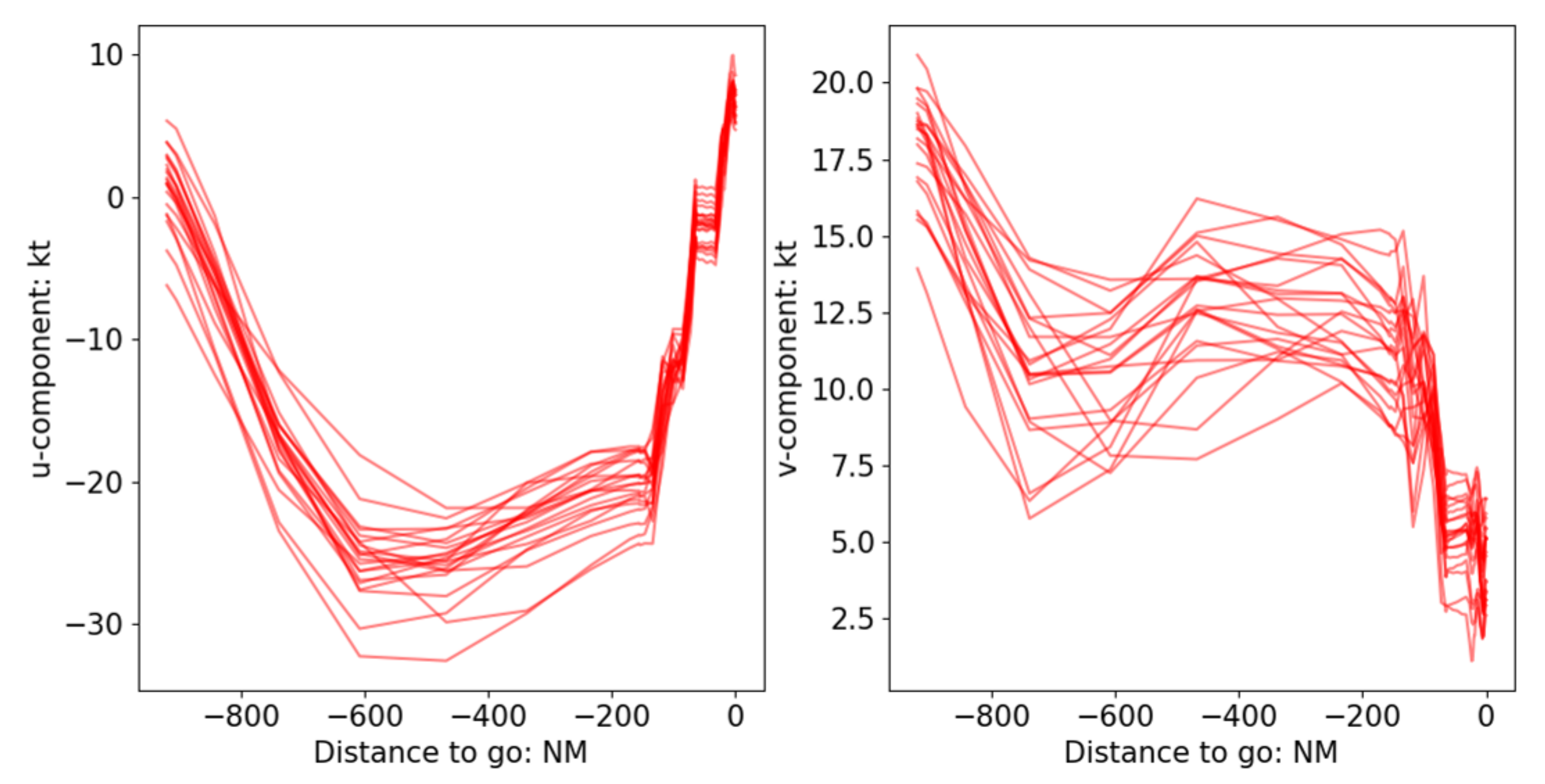
2.1. Uncertainty Models of Weather Prediction

The present study deals with uncertainties in weather prediction, which cause errors between the forecast and the true weather that the aircraft actually experiences during its flight execution. In order to model those uncertainties, we utilize the weather forecast data from the so-called Global Ensemble Forecast System (GEFS). It is a set of weather forecast scenarios provided by the National Oceanic and Atmospheric Administration (NOAA) [34] and is available online. We use version 11.0 for the present study (the newer version, 12.0, was released recently with 32 ensemble members). GEFS consists of 21 separate weather forecasts called weather ensemble members (Figure 1). Each member is obtained by perturbing the initial conditions of the weather dynamics to represent uncertainties in the meteorological models used for the forecast [35]. Small perturbations in the initial conditions evolve and lead to different weather states. The forecasts are updated every 6 h. A detailed investigation of GEFS and its application to cruise-trajectory planning can be found in [17]. The data are provided in a GRIdded Binary (GRIB2) format, which involves three dimensional grids specified by latitude, longitude and pressure level. The grid resolution is 1 for the latitude and the longitude, and 50 hPa for the pressure level.
We utilize the GEFS data to obtain the ambient temperature T m p , the pressure p and the wind speed vector, which holds the horizontal components u and v. The wind-speed components are positive for the west-to-east wind flow and the south-to-north flow, respectively. GEFS does not contain the vertical wind component. When creating the weather models, we make the following assumptions:
Assumption 1
(Horizontal wind field). We assume the wind field only has horizontal components and ignore the vertical one. This assumption is justified as the vertical component is usually one order of magnitude lesser than the horizontal components [36].
Assumption 2
(Stationary atmosphere). We assume the atmosphere is stationary; i.e., its time evolution is not considered. Therefore, the atmospheric quantities, i.e., the wind components, the temperature, the pressure and the density, are treated as functions of the aircraft 3D position.
Under these assumptions, the GRIB2-style data of GEFS are symbolically expressed as:
u G = u G ϕ G , λ G , p G , v G = v G ϕ G , λ G , p G , T m p G = T m p G ϕ G , λ G , p G ,
where ϕ and λ are the latitude and longitude in degrees, respectively; and the subscript G denotes the quantities are for a grid point. We interpolate these discrete data so that the weather model will be available at any aircraft position, or any combination of ( ϕ , λ , h). We use the three dimensional b-spline function denoted with Equation (A1) for interpolation (see Appendix A).
One remark for integrating these weather models into trajectory planning is that the aircraft dynamics normally use the geometric altitude h instead of the pressure level p to describe the height (see Section 2.2). Therefore, we need a conversion law between the two quantities. To this end, we use the conversion formula that NOAA officially provides:
p h = 1013.25 × 1 0.0065 288.15 h 5.2561 .
It is worth noting that this conversion is equivalent to assuming the International Standard Atmosphere (ISA) for the air pressure [37]. If we apply Equation (2) to substitute p in Equation (A1), the b-spline weather model for the w-th member of the weather ensemble can be rewritten as functions of the aircraft 3D position: f b s ( w ) ( ϕ , λ , p ( h ) ) . We apply this b-spline interpolation to each member of GEFS to obtain member-specific weather models (Figure 1). The b-spline-based weather models for the weather scenario w are symbolically expressed as:
u ( w ) ϕ , λ , h = u b s ( w ) ϕ , λ , p ( h ) v ( w ) ϕ , λ , h = v b s ( w ) ϕ , λ , p ( h ) T m p ( w ) ϕ , λ , h = T m p b s ( w ) ϕ , λ , p ( h ) for w = 1 , , N w .
The air density ρ , also required for trajectory calculation, can be obtained by the gas equation
ρ ( w ) ϕ , λ , h = p h R T m p ( w ) ϕ , λ , h ,
where R = 287.058 J kg 1 K 1 is the gas constant of dry air.

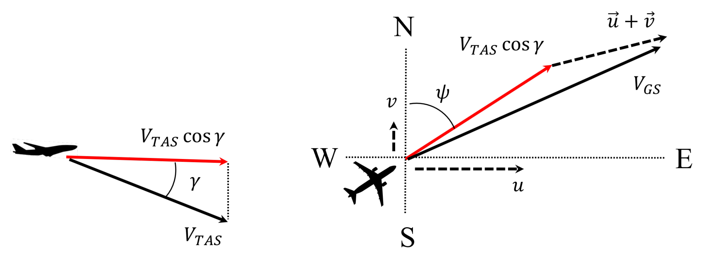
2.2. Flight Performance Models

We consider an aircraft as a dynamic system whose states are governed by the point-mass EoMs and are controlled through control inputs. When deriving the EoMs, we make the following assumptions.
Assumption 3
(Geodetic coordinate system). We express the aircraft position in the geodetic coordinates, where the aircraft position is specified with the angular coordinates, i.e., ϕ and λ, and the vertical position parameter, i.e., h. (Three different coordinate systems are usually used as reference frames fixed to the elliptical earth. They include the geodetic coordinates, the earth-centered earth-fixed Cartesian coordinates and the earth-surface Cartesian coordinates [38]. The third system is often referred to as the north–east–down (NED) coordinates, since normally its x-axis points to the north, its y-axis to the east and its z-axis downward.) This coordinate system is selected to align the aircraft dynamics with the weather model (Section 2.1). The components of wind u and v are positive for the west-to-east wind flow and the south-to-north flow, respectively.
Assumption 4
(WGS-84 Earth model). We utilize the WGS-84 Earth model defined by National Imagery and Mapping Agency (NIMA) [39]. It is an ellipsoidal earth model and is widely used for Flight Management System (FMS) [40]. The derivation of the aircraft EoM for this earth model is beyond the theme of this publication (see [38] for details).
Assumption 5
(Engine thrust is controlled by the thrust coefficient). We employ the Base of Aircraft Data family 4 (BADA4) engine thrust model [41], where the thrust T is parametrized with the thrust coefficient C T and p:
T = T C T , p .
We treat C T as a control variable representing thrust control and limit it to the following range:
C T i d l e ( M , p ) C T C T M C R Z ( M , p ) ,
where C T i d l e and C T M C R Z are the thrust coefficients for the idle and the maximum-cruise engine ratings for turbofan engines. They are functions of Mach number M and p.
Under these hypotheses, the aircraft’s 4D dynamics are expressed as:
d d t V T A S , γ , ψ , ϕ , λ , h , m T = f V , f γ , f ψ , f ϕ , f λ , f h , f m T ,
where
f V = T D m g sin γ , f γ = L cos ϕ b m g cos γ m V T A S , f ψ = L sin ϕ b m V T A S cos γ ,
f ϕ = V T A S cos γ cos ψ + v R ϕ + h , f λ = V T A S cos γ sin ψ + u ( D ϕ + h ) cos ϕ , f h = V T A S sin γ ,
f m = F C .
The aircraft state variables are x = V T A S , γ , ψ , ϕ , λ , h , m T , where V T A S is the true air speed (TAS), γ is the flight path angle, ψ is the heading and m is the gross mass. The control inputs, needed to close the set of differential equations, are u = C T , ϕ b , C L , δ S B T , where ϕ b is the bank angle, C L is the lift coefficient and δ S B is the speed brake control. R ϕ stands for the radius of curvature of the meridian’s ellipse [38] and D ϕ for the radius of curvature in the prime vertical [39] of the WGS-84 Earth model given as a function of ϕ :
R ϕ ϕ = a ( 1 e 2 ) ( 1 e 2 sin 2 ϕ ) 3 / 2 , D ϕ ϕ = a ( 1 e 2 sin 2 ϕ ) 1 / 2 ,
where a = 6.378 × 10 6 m is the equatorial radius and e = 8.18 × 10 2 is the eccentricity. D is the drag force and is written as:
D = 1 2 ρ V T A S 2 S C D clean + C D S B δ S B ,
where S is the area of the wing, C D clean is the drag coefficient in the clean configuration and C D S B is the coefficient of the speed brake effect. The two coefficients are taken from BADA4 [41]. The second term on the right-hand side of Equation (10) represents the effect of speed brake control on drag. We neglect the effect of flap and slat controls. F C represents the fuel consumption and we used the BADA4 model: F C = F C ( V T A S , C T , p , T m p ) .
To simplify the aircraft dynamics and make the problem easier and faster to solve, we make additional assumptions.
Assumption 6
(Heading as a control input). We assume ψ can be changed instantaneously instead of following the rotational dynamics (Equations (7) and (8)). We neglect the corresponding dynamics and treat ψ as a control variable, since it still appears in other dynamics (Equation 8). This also allows us to ignore ϕ b and remove it from the control inputs.
Assumption 7
(Vertical equilibrium). We assume the vertical forces acting on the aircraft are balanced:
L = m g cos γ .
This assumption leads to d γ / d t = 0 in Equation (7) and allows us to neglect the γ-dynamics. γ is excluded from the state variables and we include it in the control inputs instead. This type of model is called the γ-command model and is widely used for trajectory calculation for ATM purposes [13,15,42,43,44]. It also allows us to remove C L from the control inputs. This is because C L can be calculated automatically if γ is specified in Equation (11) as:
C L = 2 L ρ V T A S 2 S = 2 m g cos γ ρ V T A S 2 S .
Under these assumptions, the EoMs are simplified as
d d t V T A S , ϕ , λ , h , m T = f V , f ϕ , f λ , f h , f m T ,
where the aircraft state variables are x = { V T A S , ϕ , λ , h , m } T and the control variables are u = { C T , γ , ψ , δ S B } T .
Currently, we have the time t as the independent variable for our formalization. From the optimal control viewpoint, this means t is required to be in the same domain [ t 0 , t f ] for any of the state variables. In other words, the initial time t 0 and the final time t f must be the same for the trajectories of any state and control variables. As we discuss in Section 3.2, we eventually aggregate the EoM to cover the dynamics for all the weather scenarios to create a robust optimal control problem. t being in the same domain means the arrival time at the final position must be common for any member of the trajectory ensemble. However, this is normally not true. A different weather situation, especially a different wind speed, causes different ground speed, and consequently the arrival time should be varied. Therefore, we need a different independent variable to properly model the variations in trajectory with respect to time. We make the following assumption:
Assumption 8
(Along-track distance as the independent variable). Instead of t, we treat the along-track distance s, another strictly increasing variable, as the independent variable. As seen in Figure 2, s is defined as the distance along the aircraft path projected onto the earth surface and expressed using the ground speed V G S :
s = t 0 t f V G S d t ,
where V G S is expressed as:
V G S = ( V T A S cos γ cos ψ + v ) 2 + ( V T A S cos γ sin ψ + u ) 2 .
The feature of s being in the same domain [ s 0 , s f ] for any member of trajectory ensemble is justified by the commonality constraints we will introduce in Section 3.2, which require the aircraft to fly the common 3D route regardless of the weather scenario. The selection of s as the alternative independent variable can also be seen in prior studies [28,43,44]. We perform this transformation, applying the chain rule d / d t = d / d s · d s / d t . Here, d s / d t = V G S due to Equation (14), and therefore the time derivative can be written as d / d t = V G S · d / d s . Applying this formula to Equation (13), we can change the independent variable from t to s. This conversion removes t from the EoMs. Instead, we treat it as an additional state variable and include its evolution in the set of EoMs. The resulting EoMs are:
d d s V T A S , ϕ , λ , h , m , t T = 1 V G S f V , f ϕ , f λ , f h , f m , 1 T ,
where the independent variable is s, the state variables are x = { V T A S , ϕ , λ , h , m , t } T and the control variables are u = { C T , γ , ψ , δ S B } T . We use these EoMs for the robust trajectory planning. For facilitating the following discussion, we define the aircraft dynamics vector as f = { f V , f ϕ , f λ , f h , f m , 1 } T / V G S .

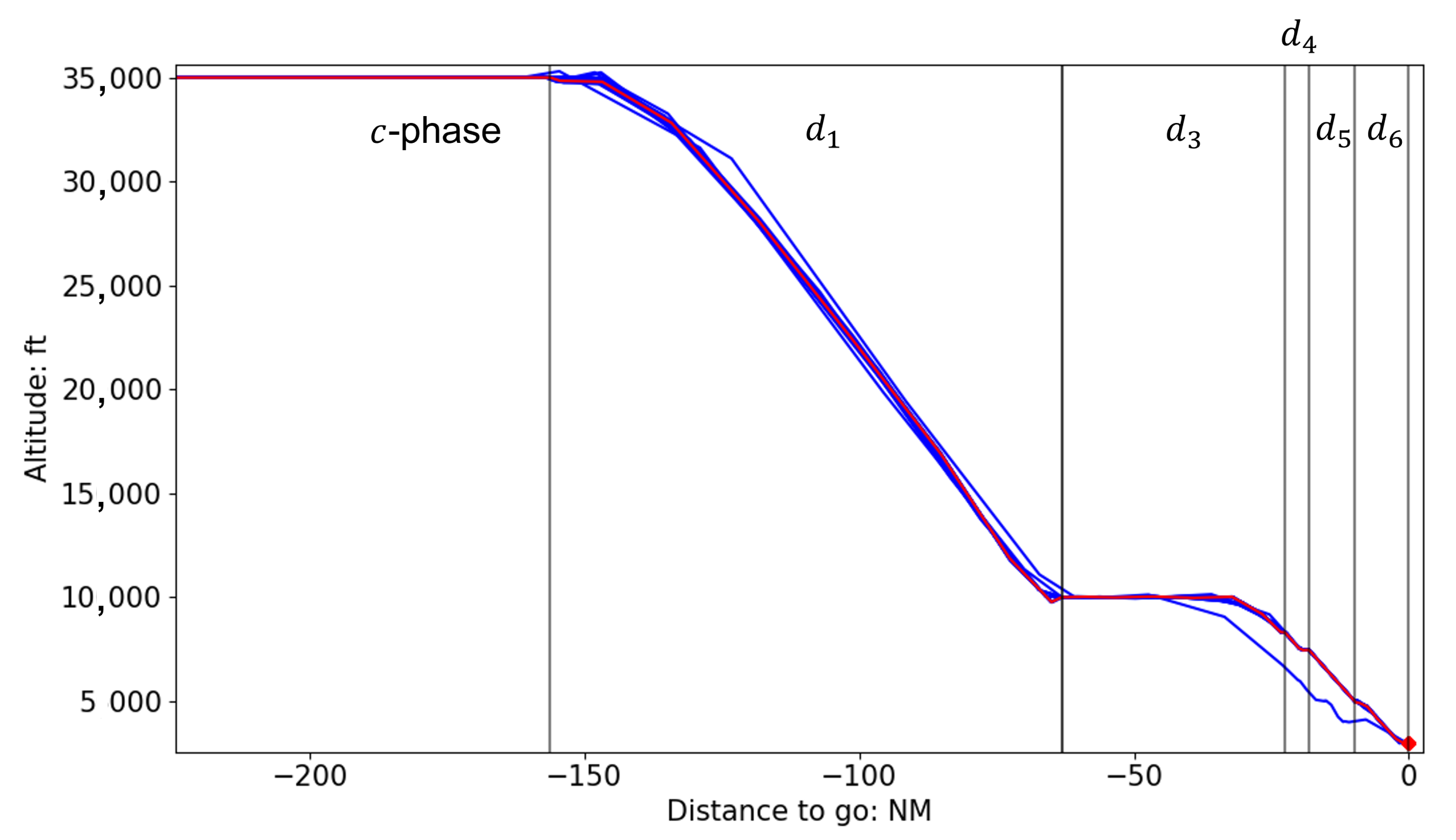
3. Robust Descent Trajectory Planning

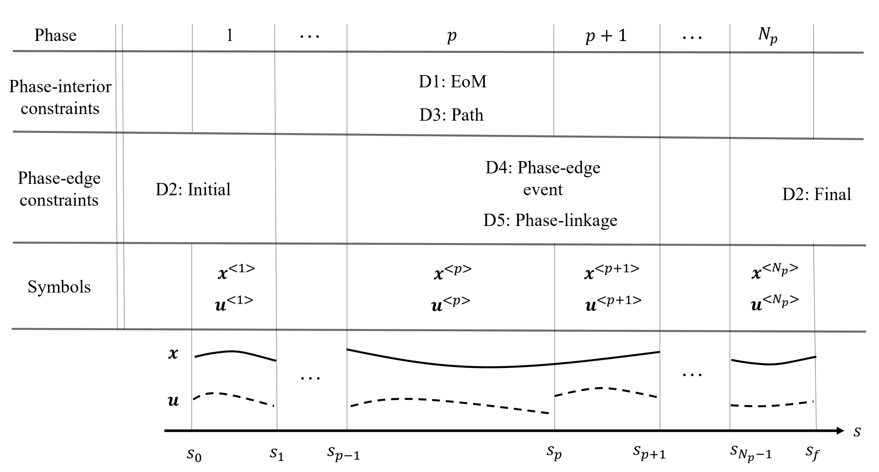
3.1. Deterministic Formalization as a Basis

Before formalizing a robust trajectory planning problem, we first create the corresponding deterministic problem to be a basis of the robust formalization. We split the trajectory into phases so that we can consider phase-specific constraints, and we express the total number of phases with N p . An overview of the phase-specific constraints and symbols is summarized in Figure 3. To deal with these phases, we apply the multiple-phase optimal control theory to the planning problem [33,45]. The variables in the optimal control problem are the state vector x and the control vector u , and the independent variable s. We add the superscript < p > to x or u to denote the variable is for the phase p ( = 1 , , N p ). s 0 and s f are used to represent the s of the initial and final positions, respectively. We also use s p to describe the s of the edge between the p-th and the p + 1 -th phases. According to the definition, s f and s N p are equal.
The deterministic multiple-phase optimal control problem consists of the following constraints. We discuss them using generic expressions in this section and show the details in Section 4.1.
Constraint D1: Aircraft EoM
The aircraft trajectory for the phase p is expressed as a set of differential equations:
d x < p > d s = f x < p > , u < p > for p = 1 , , N p .
We assume f to be unchanged across the considered phases.
Constraint D2: Initial/final conditions
The initial and final conditions can be specified as:
g i n i t x < 1 > ( s 0 ) = 0 , g f i n x < N p > ( s f ) 0 ,
where g i n i t and g f i n are sets of functions defining the initial and final conditions, respectively. The final conditions are allowed to be inequality constraints.
Constraint D3: Path constraints
The path constraints define limitations inside each phase, not at the phase edges:
g l o w < p > g p a t h < p > x < p > , u < p > g u p < p > for p = 1 , , N p ,
where g p a t h < p > is a set of functions defining the constraints, and g l o w < p > and g u p < p > are the corresponding lower and upper bounds. The path constraints include operational limitations, e.g., CAS and altitude limitations, representing the flight envelope and the arrival route structure.
Constraint D4: Phase-edge event conditions
The event conditions represent requirements the trajectory has to meet at phase edges:
g e v e n t < p > x ( s p ) 0 for p = 1 , , N p 1 .
These conditions typically represent speed and altitude limits at waypoints.
Constraint D5: Phase-linkage conditions
The phase-linkage conditions are specific to multiple-phase formalization and connect the trajectories of the state variables at each phase edge, ensuring continuity of trajectory:
x < p > ( s p ) x < p + 1 > ( s p ) = 0 for p = 1 , , N p 1 .
If we define g l i n k a g e < p > = x < p > ( s p ) x < p + 1 > ( s p ) , the linkage conditions are expressed as:
g l i n k a g e < p > x < p > , x < p + 1 > , s p = 0 for p = 1 , , N p 1 .
This study does not impose these conditions on the control inputs. This means we allow instant change of control at phase edges.
With the above constraints, we aim to minimize the following objective functional.
Objective: Minimum operational costs
We set operational costs as the objective for the deterministic planning to minimize: J d e t (€). The operational costs are defined as a combination of the time-related costs J t i m e (€) and the fuel costs J f u e l (€). The time-related costs are defined as the costs charged for the flight time for the considered flight phases represented by the final time t < N p > ( s f ) . A linear relationship is assumed between the time costs and the final time through the coefficient C t i m e (€/s) as: J t i m e = C t i m e t < N p > ( s f ) . We model the coefficient utilizing the cost index C I = 60 · C t i m e / C f u e l (kg/min) (the unit is aligned Airbus’s C I definition [46]), where C f u e l (€/kg) denotes the jet fuel price. If we substitute C t i m e with C I , we obtain
J t i m e = C I C f u e l 60 t < N p > ( s f ) .
On the other hand, we define the fuel costs as the costs charged for the fuel burn F B (kg) for the considered flight phases: J f u e l = C f u e l F B . The fuel burn can be expressed as the difference between the initial and the final aircraft mass: F B = m < 1 > ( s 0 ) m < N p > ( s f ) , as shown in Appendix B. Thus, the fuel costs are written as:
J f u e l = C f u e l m < 1 > ( s 0 ) m < N p > ( s f ) ,
leading to:
J d e t = J t i m e + J f u e l = C f u e l C I 60 t < N p > ( s f ) + m < 1 > ( s 0 ) m < N p > ( s f ) .
To summarize, the deterministic multiple-phase optimal control problem is expressed as:
Find u < 1 > , , u < N p > , s 1 , , s f min operational cos ts Equation ( 25 ) subject to aircraft EoM Equation ( 17 ) initial / final conditions Equation ( 18 ) path constraints Equation ( 19 ) phase - edge event conditions Equation ( 20 ) phase - linkage conditions Equation ( 22 )
To facilitate the following discussion, we rewrite the optimal control problem further. We gather the variables for all phases into a single vector as x ˜ = { x < 1 > , , x < N p > } T , u ˜ = { u < 1 > , , u < N p > } T to cover the entire trajectory. We use the tilde symbol to denote the variables covering all the phases. Using this all-phase expression, the EoM can be expressed as:
d x ˜ d s = f x ˜ , u ˜ .
If we also apply the all-phase principle with the tilde symbol to the path constraints, the phase-edge event condition and the phase-linkage conditions, they are rewritten as:
g ˜ l o w g ˜ p a t h x ˜ , u ˜ g ˜ u p ,
g ˜ e v e n t x ˜ , s 1 , , s N p 1 0 ,
g ˜ l i n k a g e x ˜ , s 1 , , s N p 1 = 0 .
As a result, the deterministic optimal control is finally expressed as:
Find u ˜ , s 1 , , s f min operational cos ts Equation ( 25 ) subject to aircraft EoM Equation ( 26 ) initial / final conditions Equation ( 18 ) path constraints Equation ( 27 ) phase - edge event conditions Equation ( 28 ) phase - linkage conditions Equation ( 29 )

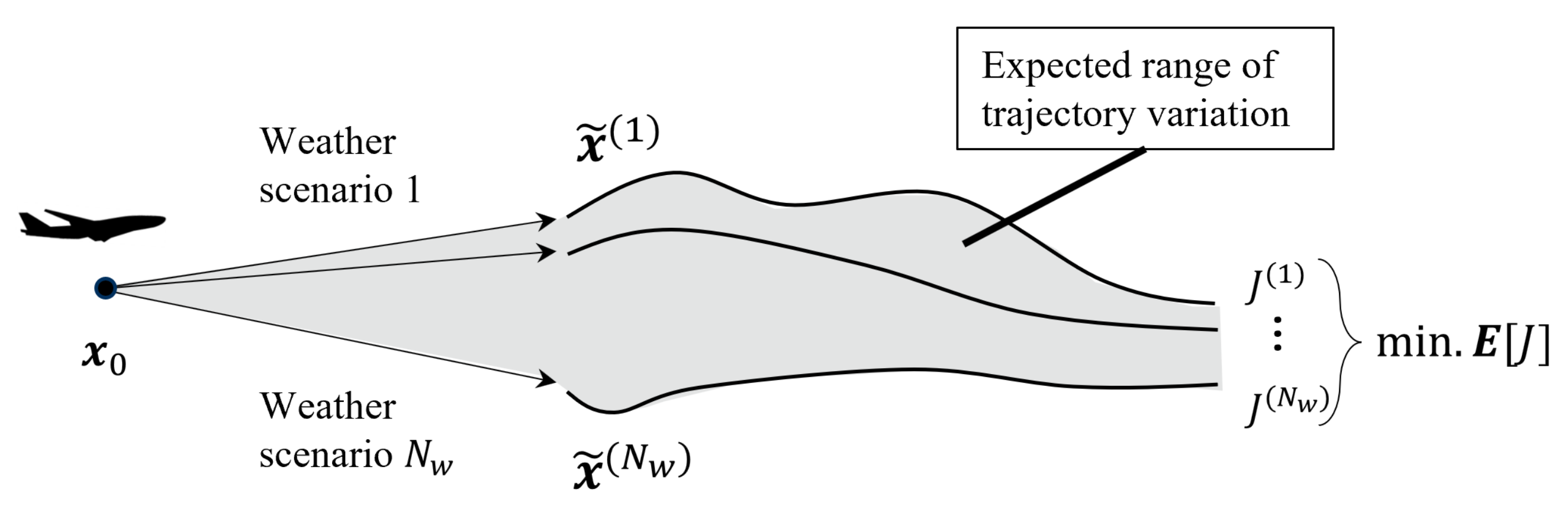
3.2. Robust Trajectory Planning
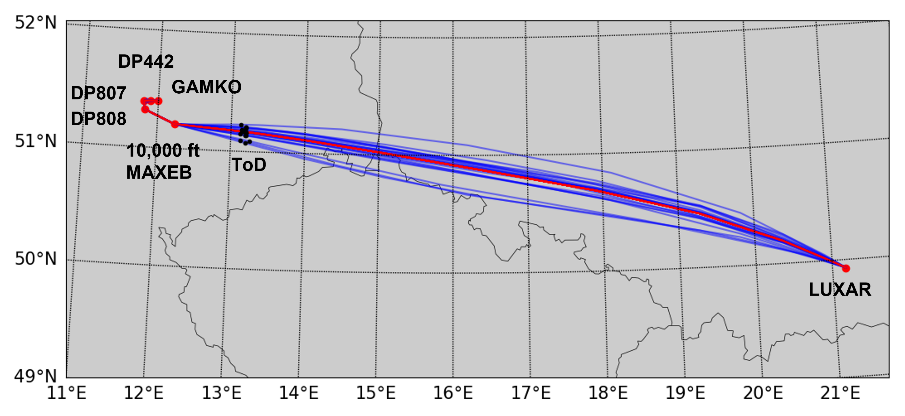
In the development of robust optimization, several types of measure of robustness have been proposed [47]. The most common measure is achieved by optimizing the problem for the worst case among the anticipated scenarios. This strategy takes a scenario that produces the highest costs and optimizes the problem for it. Such costs are expressed with the max function, and thus this type of method is also called the min–max method. However, a solution optimized for the worst case, which usually happens rarely, is often too conservative for the other cases, which are more probable. To deal with this issue, another definition of robustness has also been proposed. It regards a robust solution as the one that is optimized for the moments of the overall costs covering any realization of the uncertainty sets: such as the expected value (the first moment) or the variance (the second moment), or even higher moments [28]. This study takes the latter definition and optimizes the trajectory in terms of the expected value of the operational costs.
We formulate the robust planning problem based on the deterministic formalization discussed in Section 3.1. We take a set of N w GEFS members as possible realizations of the uncertain weather during the flight. We define robust trajectories as (1) trajectories that are feasible in any GEFS weather scenarios in the sense that they do not violate the operational limitations, and (2) trajectories that are optimized for the expected value of the costs. Feasibility of the trajectories is achieved by making the EoM and the operational limitations hard constraints regardless of weather conditions within the uncertainty range provided by GEFS data. We apply robust optimal control similarly to [28,33]. Unlike prior works, such as [26], assuming common control inputs to different weather scenarios, we basically consider that both the aircraft states and control inputs are different for different weather scenarios. We explicitly express the variables as x ˜ ( w ) , u ˜ ( w ) with the superscript to show the variables are for the weather scenario w. On the contrary, we assume the independent variable s are in a common domain s [ s 0 , s f ] for any w. We also assume s p for the intermediate phase edges p = 1 . , N p 1 are common to the different weather scenarios. Therefore, s, s 0 , s f and s p s do not need the superscript.
The robust optimal control problem holds the following constraints based on the corresponding deterministic constraints.
Robust constraint R1: Aggregated aircraft EoM
We apply the deterministic EoM (Equation (26)) to each weather scenario w = 1 , , N w as d x ˜ ( w ) / d s = f ( x ˜ ( w ) , u ˜ ( w ) ) . We assume the aircraft dynamics do not change across scenarios, and therefore f does not need the superscript. We call this set of N w trajectories the trajectory ensemble. The trajectory for the weather scenario w is the w-th member of the trajectory ensemble. Then we aggregate the set of EoMs as:
d d s x ˜ ( 1 ) x ˜ ( N w ) = f x ˜ ( 1 ) , u ˜ ( 1 ) f x ˜ ( N w ) , u ˜ ( N w ) .
We call this set of EoMs aggregated aircraft EoM. With this aggregated dynamic constraint, the trajectory ensemble is computed and optimized simultaneously.
Robust constraint R2: Commonality constraints
If we solve the aggregated EoM, a different trajectory is calculated for each weather scenario. From the operational point of view, however, such a set of trajectories will make pilots unsure about which trajectory to follow, as they do not know which weather scenario to expect. To give them single reference, this study proposes the commonality constraints limiting the aircraft’s 3D positional trajectories ϕ ˜ ( s ) , λ ˜ ( s ) and h ˜ ( s ) common to all weather scenarios:
ϕ ˜ ( w ) ( s ) = ϕ ˜ ( 1 ) ( s ) , λ ˜ ( w ) ( s ) = λ ˜ ( 1 ) ( s ) , h ˜ ( w ) ( s ) = h ˜ ( 1 ) ( s ) for w = 2 , , N w .
These commonality constraints let the problem be different from just repeating the deterministic optimization N w times, as each of the trajectory ensemble members needs to share the common positional profile and thus cannot be optimized individually.
Robust constraint R3: Initial/final conditions
We assume the trajectory planning starts with the common initial aircraft state regardless of the weather scenario. Considering Equation (18), the initial aircraft state x ˜ ( w ) ( s 0 ) and the final state x ˜ ( w ) ( s f ) must satisfy:
g i n i t x ˜ ( w ) ( s 0 ) = 0 , g f i n x ˜ ( w ) ( s f ) 0 for w = 1 , , N w .
g i n i t and g f i n without the superscript ( w ) mean these functions are independent of w.
Robust constraint R4: Path constraints
We apply Equation (27) to each weather scenario w
g ˜ l o w g ˜ p a t h x ˜ ( w ) , u ˜ ( w ) g ˜ u p for w = 1 , , N w .
The path constraints, including the flight envelope, operational limitations, etc., are hard and must be met regardless of the weather scenario. Therefore, the lower and upper bounds are independent of the weather scenario w.
Robust constraint R5: Phase-edge event conditions
The events at phase edges, such as speed and altitude limitations, must be hard constraints as well. Based on Equation (28), the constraints are expressed as:
g ˜ e v e n t x ˜ ( w ) , s 1 , , s N p 1 0 for w = 1 , , N w .
Robust constraint R6: Phase-linkage conditions
The continuity of the trajectory at any phase edge is naturally required for any weather scenario. Considering Equation (29), the robust linkage conditions are:
g ˜ l i n k a g e x ˜ ( w ) , s 1 , , s N p 1 = 0 for w = 1 , , N w .
In addition to the above constraints, we introduce an additional constraint related to the arrival time at the final state.
Robust constraint R7: Required time of arrival
We consider the required time of arrival (RTA) for the final position. The trajectories of t are uncommon to trajectory ensemble members and therefore the final time t < N p > ( w ) ( s f ) is different for each w. We define the robust RTA as a constraint for the expected value of the arrival time: E [ t < N p > ( s f ) ] = t R T A , where the time constraint t R T A is a given parameter. This study assumes each GEFS member is equally probable. Under this assumption, this constraint is:
1 N w w = 1 N w t < N p > ( w ) ( s f ) = t R T A .
We also derive the robust objective functional based on the deterministic one.
Robust objective: Expected value of the operational costs
As discussed above, we minimize the expected value of the operational costs:
J r o b u s t = E J d e t = C f u e l N w w = 1 N w C I 60 t < N p > ( w ) ( s f ) + m < 1 > ( w ) ( s 0 ) m < N p > ( w ) ( s f ) .
To summarize the discussion, the robust optimal control problem for robust trajectory planning can be described as:
Find u ˜ ( 1 ) , , u ˜ ( N w ) , s 1 , , s f min expected operational cos ts Equation ( 37 ) subject to aggregated aircraft EoM Equation ( 30 ) commonality constraints Equation ( 31 ) initial / final conditions Equation ( 32 ) path constraints Equation ( 33 ) phase - edge event conditions Equation ( 34 ) phase - linkage conditions Equation ( 35 ) required time of arrival Equation ( 36 )
Figure 4 shows the overview of the process of the proposed robust planning strategy. The trajectory optimization starts with the common initial state x 0 and each weather scenario is applied to the corresponding part of the aggregated EoM to make the members of the trajectory ensemble. The ensemble can provide the expected range of trajectory variation. Each ensemble member leads to its own value of the objective, and we minimize the mean value. This means of optimization simultaneously considers N w members of the trajectory ensemble.
It is well known that optimal control problems generally do not have closed-form analytic solutions, except for a few known, simplified problems, such as the linear quadratic optimal control problem [48]. We utilize the co-called pseudospectral method, a numerical computation method where the continuous optimal control problem is discretized into so-called pseudospectral nodes. Among several kinds, we take the Legendre–Gauss pseudospectral method (LGPM). The resulting discrete optimization problem is categorized as a nonlinear programming (NLP) problem, for which a variety of solvers are widely available. We utilize IPOPT (interior point optimizer) [49], an open-source software package for large-scale nonlinear optimization. We use an open-source optimization tool CasADi [50] to interface IPOPT with Python. An equal number of pseudospectral nodes is assumed in this study for any phase p.

4. Case Studies

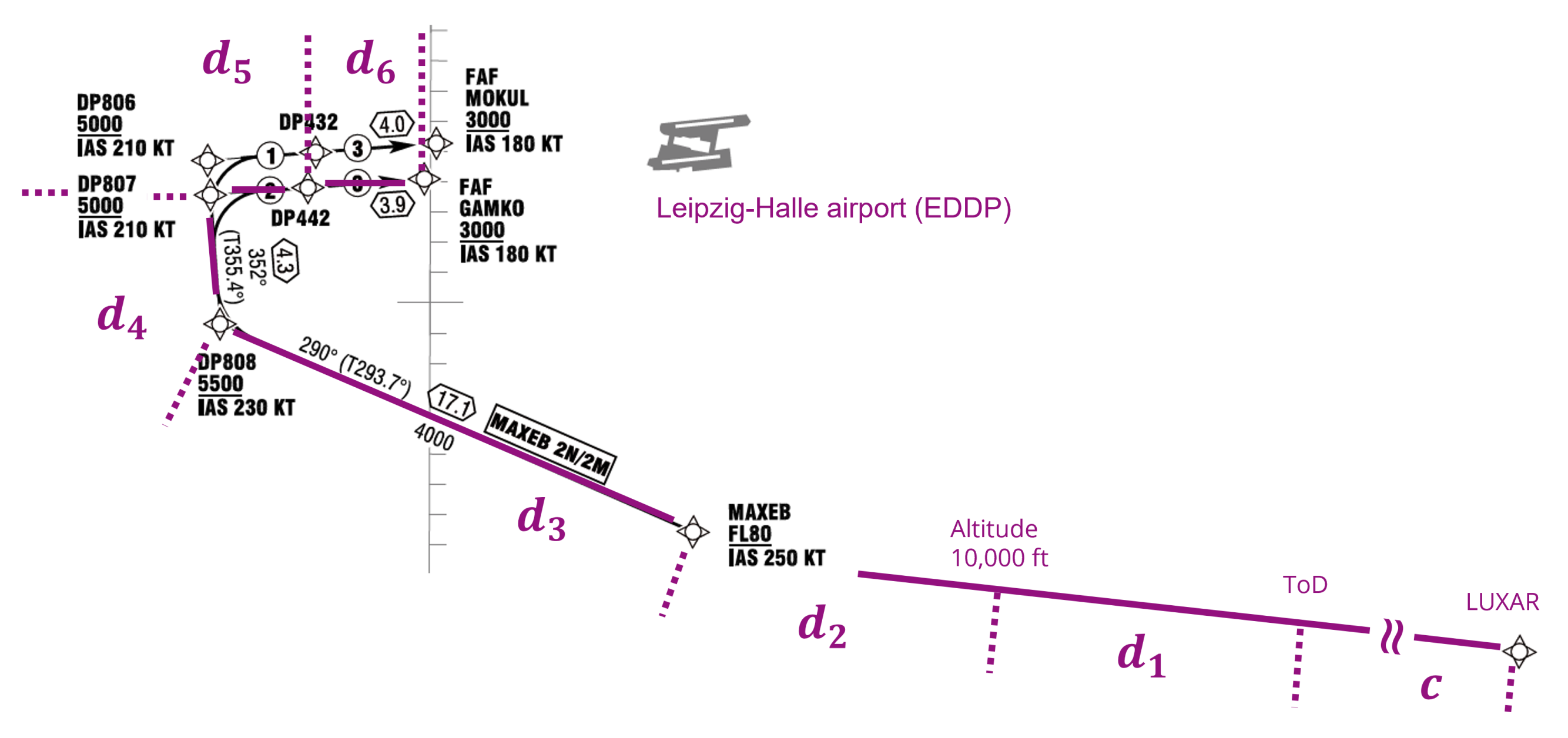
4.1. Scenario Settings

We apply the proposed planning algorithm to an aircraft descending to Leipzig/Halle Airport in Germany (ICAO code: EDDP) through the transition procedure for runway 08R (Figure 5). This transition route is designed for CDO operation and used only at night time (CDO NIGHT). The relevant waypoints are listed in Table 1.
The optimal trajectory is calculated from the en-route waypoint LUXAR, and the initial conditions for the simulation are as listed in Table 2. In the initial state, the aircraft is assumed to pass LUXAR with level flight at a cruising altitude of 35,000 ft with 63,700 kg of total mass. We split the descent trajectory into several phases. We take the relevant waypoints as phase edges that the aircraft flies over, though they are actually defined as fly-by waypoints. The phase-specific constraints for the optimization are listed in Table 3. We require the CAS to stay slower than 250 kt below 10,000 ft. This constraint comes from the FAA regulation (14 CFR § 91.117). M M i n and M M O are the minimum Mach number and the maximum operating Mach number, respectively.
In addition to the phase-specific constraints, we also have inter-phase limitations for the control inputs as described in Table 4. In the table, C T i d l e and C T M C R Z are the thrust coefficients for the idle rating and maximum-cruise rating. To calculate the constraints in Table 3 and Table 4, we utilize BADA4’s CAS model for V C A S ; the thrust coefficient models for C T i d l e and C T M C R Z ; and the values of minimum/maximum Mach number for M m i n and M M O [41]. We take the GEFS data published on the September 22nd, 2020 at 0:00. We use 746.73 $/ton for the jet fuel price published by IATA [52] for October 8th, 2021. With relevant unit changes, the unit fuel costs are calculated as C f = 0.64 €/kg.

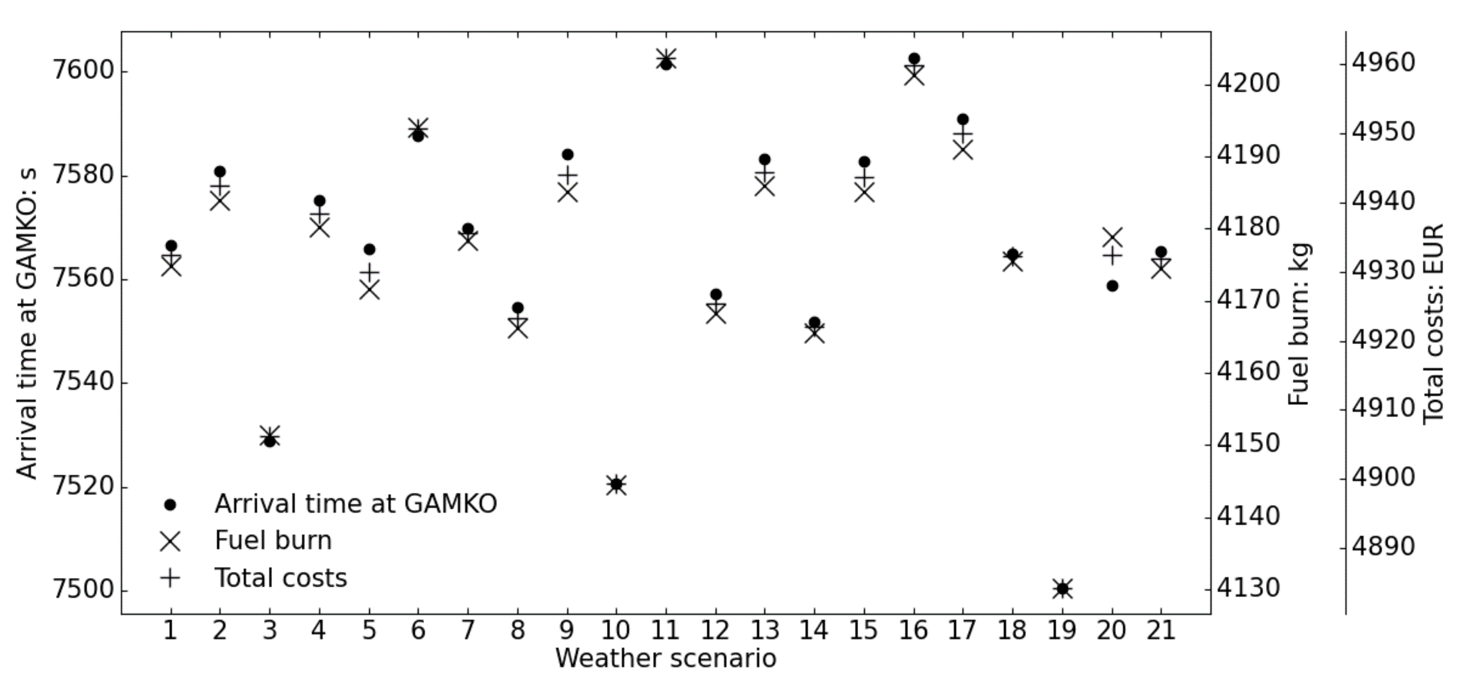
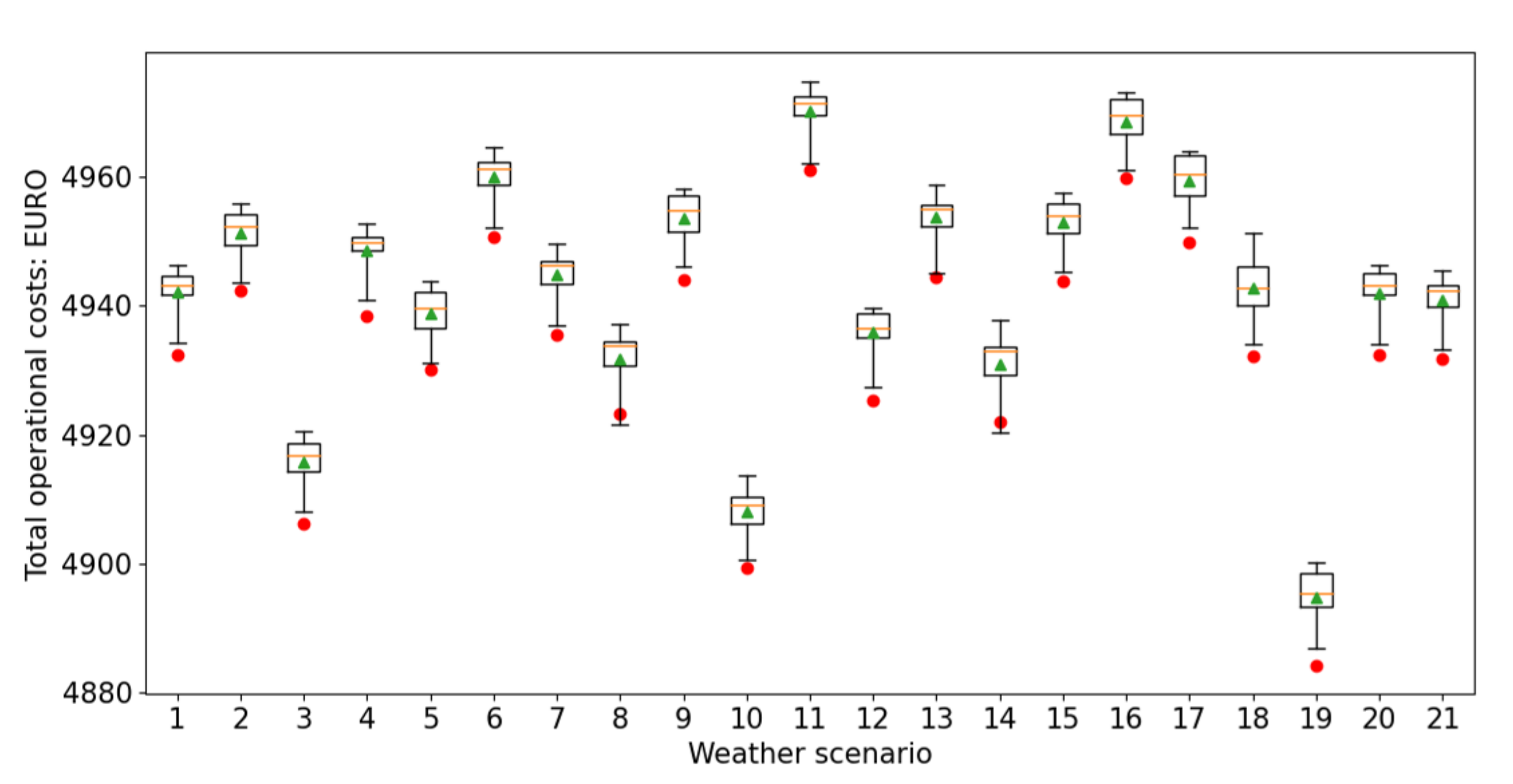
4.2. Robust vs. Scenario-Optimal Trajectories

In order to validate the proposed planning algorithm, we calculate deterministic trajectories optimized for each weather ensemble member. We call these trajectories scenario-optimal trajectories. They are obtained by applying the deterministic planning algorithm (Section 3.1) to each weather scenario.
Figure 6 shows the lateral paths of the robust (in red) and the scenario-optimal (in blue) trajectories for the case with C I = 30 kg/min without RTA, together with the waypoints and the ToD locations, and Figure 7 shows the wind speed components along the robust trajectories. Both robust and scenario-optimal trajectories reach 10,000 feet altitude at MAXEB, so the end of d 1 phase and the beginning of d 3 phase are found to be equal. With these variations in u and v trends, the scenario-optimal trajectories are varied between LUXAR and MAXEB, whereas the robust trajectories share the common lateral path due to the commonality constraints (Section 3.2). This single weather-scenario-independent path facilitates the pilot following the trajectory plan no matter the weather, which is one of the benefits of the proposed robust planning strategy. N w repeats of the scenario-optimal deterministic planning is not able to calculate such trajectories. There was no significant difference in lateral path found after MAXEB.
The corresponding vertical trajectories are shown in Figure 8. Gaps between the robust and the scenario-optimal trajectories are mainly in the d 1 phase except for a case where the aircraft flies lower in the following descent phases. A temporary horizontal segment is shown in the d 3 phase, where the aircraft flies from MAXEB at 10,000 ft height to DP808. This is mainly due to the corresponding altitude restriction. The altitude is limited between 5500 ft and 10,000 ft in this phase, and the optimal trajectories maintain 10,000 ft, the highest altitude allowed, as long as it is possible to minimize the drag.
Figure 9 depicts the arrival time at GAMKO, fuel burn and operational costs that the robust trajectory results in for each weather scenario. The average arrival time is 7566 s and its standard deviation is 25.0 s, whereas the average fuel burn is 4176 kg and its standard deviation is 17.3 kg. These arrival times and fuel burns lead to 4933 € for the average operational costs and 18.4 € for its standard deviation.

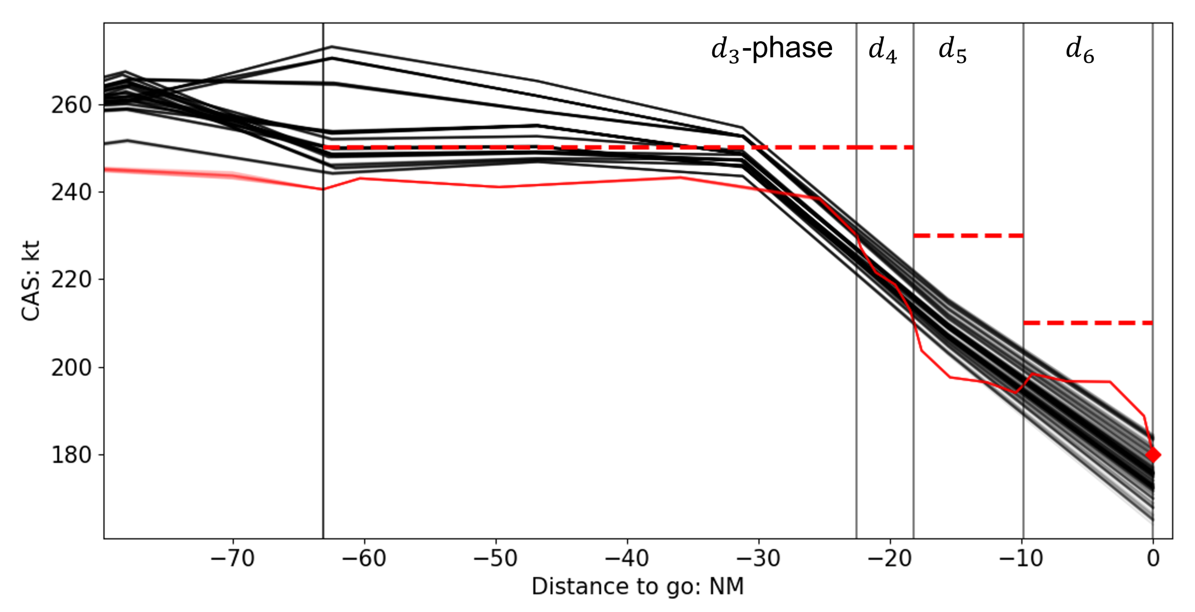
4.3. Robust vs. Inappropriately-Controlled Trajectories

We introduce another type of trajectory named the inappropriately-controlled trajectory. This is the type if the pilot follows one of the scenario-optimal trajectories in a weather scenario different from the assumed one. The inappropriately-controlled trajectories represent situations where a deterministic situation is assumed for trajectory planning and the pilot has to follow a trajectory optimized for a certain weather scenario but the true weather is different. We calculate the inappropriately-controlled trajectory for the weather scenario w by applying the scenario-optimal control inputs for the other scenarios u ˜ ( i ) ( i = 1 , , N w and i w ) . This leads to N w 1 inappropriately-controlled trajectories for each weather scenario. An inappropriately-controlled trajectory can lead to better costs than those with the robust trajectory when the assumed weather scenario i for the applied scenario-optimal control is close to the true scenario w.
Figure 10 shows the costs of the robust trajectories (red dots) and the inappropriately-controlled trajectories (box plots) for each weather ensemble member (the case with C I = 30 kg/min and RTA not imposed). The robust trajectories achieve better operational costs than the average costs of the corresponding inappropriately-controlled trajectories (green triangles) in all weather scenarios. Except for two scenarios (8 and 14) among 21, the robust trajectory even results in lower costs than any of the corresponding inappropriately-controlled trajectories. This means that the robust trajectories are expected to achieve better performances in all objectives of the optimization. Trajectories planned in a deterministic way can result in lower costs only when the assumed weather situation is close to the actual weather.
Violation of operational constraints is another issue when the pilot only has a deterministic trajectory plan. We can see some limitations and specifications for V C A S are violated in the case with C I = 20 kg/min and without RTA. Figure 11 shows the V C A S profiles of the robust and inappropriately-controlled trajectories for the d 3 , , d 6 phases. We can see the inappropriately-controlled trajectories contain higher V C A S than the robust ones, and some of them violate the 250-kt limitation in the d 3 phase. Other inappropriately-controlled trajectories fail to meet the 180-kt final condition at the end of d 6 phase. The robust trajectory meets all the constraints.

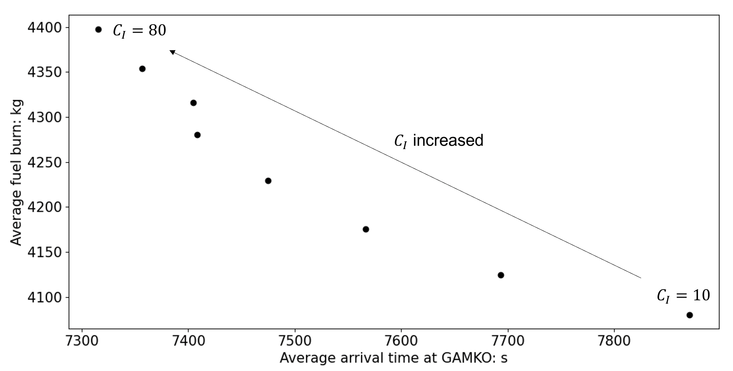
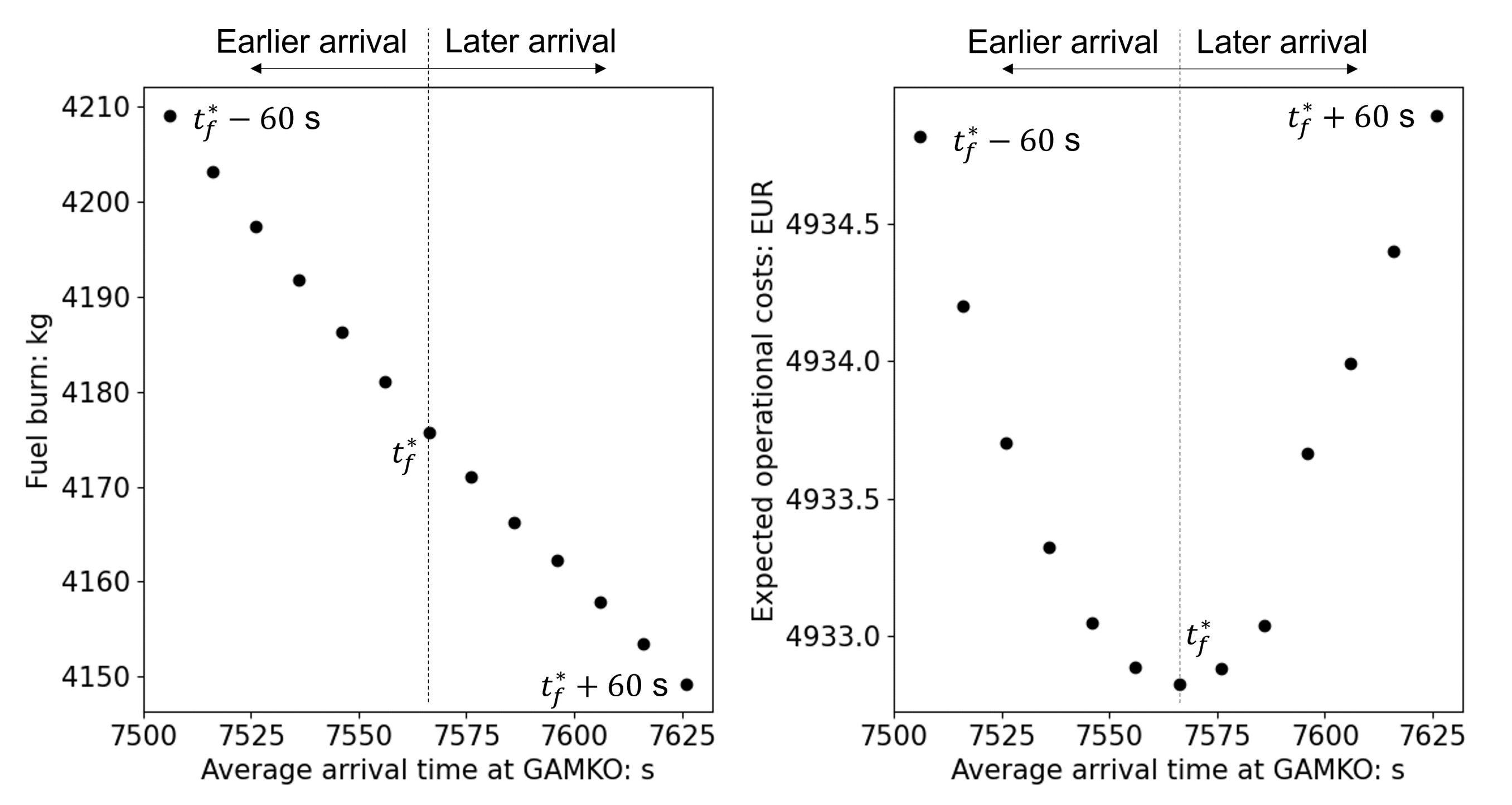
4.4. Effects of Cost-Index and RTA Variations

We also test the proposed planning framework with varied parameter settings— C I and t R T A —to investigate how robust trajectories change with their variations. We first vary C I from 10 to 80 kg/min, while not imposing RTA. Figure 12 shows the relationship between the average arrival time at the final state (GAMKO: FAF) and the average fuel burn, depending on the values of C I . When a larger C I is applied to the trajectory planning, the aircraft flies faster and arrives at GAMKO earlier to reduce the time costs. This method of flight leads to more drag and requires more thrust. Consequently, more fuel is necessary. Compared to the case with C I = 10 kg/min, the flight time is reduced by 564 s (7.2%) but with 310 kg (7.6%) more fuel being burnt at C I = 80 kg/min.
As for the RTA, we use the symbol t f * to represent the average arrival time at GAMKO of the robust trajectories without RTA imposed. We vary t R T A from t f * 60 (s) to t f * + 60 (s), and we keep C I = 30 kg/min when t R T A is varied. Figure 13 depicts the trend of the average fuel burn vs. the expected operational costs (Equation (37)) with various RTAs. Earlier arrival times than t f * require more fuel burn, whereas later arrival times require less, as the aircraft needs to increase/decrease the overall speed to meet the arrival time constraint, leading to more/less thrust, respectively. When the aircraft is required to arrive at GAMKO 60 s earlier than t f * in the trajectory plan, 33.4 kg more fuel is burnt. When the arrival time is 60 s later, the fuel burn is 26.5 kg less. In terms of the expected value of the total operational costs, the case without RTA achieves the minimum costs. When the average aircraft arrival time is required to be 60 s earlier than the optimal average arrival time t f * , the costs become 2.0 € higher than for the case without RTA. If t f * + 60 s of RTA is required, 2.1 € more costs are necessary. The change in the operational costs is much smaller than that in the arrival time and fuel burn with the formalization and the weather data we utilize for the present study. A different definition of the cost function (Equation (37)) and a different set of GEFS data could provide larger differences. Yet, as the expected trend is shown in Figure 13 (right): the case without RTA leads to the minimum costs.
Figure 12 and Figure 13 also confirm the proposed robust planning framework is able to deal with these parameter changes. The ability to carry out this type of analysis is beneficial for operators. If we interpolate the dots on Figure 12, we can obtain a curve of arrival-time and fuel-burn trend. Such a figure provides airlines with information on how much additional fuel or additional flight time they need to expect depending on their C I setting, and is helpful for determining the value of C I to take. The same kind of interpolation can also be applied to the figures in Figure 13, providing ATCs with insights on how much additional costs and fuel burn they have to impose on the aircraft with a certain value of RTA. This information allows the ATC and the pilot to negotiate for their best RTA, considering benefits for both sides.
The simulation results we have discussed so far prove that the planning algorithm can work for our scenario’s settings and weather data. In order to validate the algorithm more thoroughly, we need to test it with a variety of conditions, including weather data, arrival routes, initial conditions and C I s and RTAs. Further validation is one of the authors’ main future intentions. Study in practical applications will also be authors’ future work.

5. Conclusions

This study proposes a fundamental framework and computational algorithms for planning optimal descent trajectories that are robust against uncertainties in weather prediction. We utilized a set of weather scenarios provided by GEFS to model the uncertainties related to weather prediction. A deterministic multiple-phase optimal control problem was built to form the basis of the robust optimal control problem, considering 4D aircraft dynamics. We formalized a robust optimal control problem by aggregating the state and control variables and the aircraft dynamics for each of the weather scenarios to create an aggregated EoM. We introduced constraints characterizing the robust planning, i.e., the commonality constraints, so that the robust trajectories can have the common 3D positional profiles over the considered weather scenarios. Unlike conventional worst-case optimization, the proposed robust optimal control minimizes the expected value of the costs for the considered set of weather scenarios. We applied the proposed algorithm to descent trajectory planning for Leipzig/Halle Airport. Comparison of robust and inappropriately-controlled trajectories allowed us to confirm the proposed planning algorithm can prevent high costs and infeasible trajectories that violate operational constraints in any weather scenarios. Optimization results with different C I and RTA showed the proposed robust optimal control can cope with these varying operational settings. The analyses with different parameter settings support operators, i.e., pilots, airlines and ATCs, in determining the best values for those parameters. This study discussed a robust planning problem in a generic form and proposed a fundamental framework which can be applied to a wide range of scenario settings.
One of our main future intentions is to test the proposed planning algorithm with a variety of weather scenarios, arrival routes, initial conditions and C I and RTA settings to thoroughly validate its performance. We will also utilize the robust planning strategy to solve operation-oriented problems, such as a RTA-assignment problem for a metering FIX, where the time to reach the FIX is uncertain. In addition to these, we will apply the planning algorithm to more advanced air/space structures such as trombones and point merging to enhance its applicability.

Author Contributions

Conceptualization, S.K. and J.R.; methodology, S.K.; software, S.K.; validation, S.K. and J.R.; writing—original draft preparation, S.K.; writing—review and editing, S.K., J.R., H.F. and M.S.; visualization, S.K.; supervision, J.R., H.F. and M.S.; project administration, J.R. and H.F.; funding acquisition, H.F. All authors have read and agreed to the published version of the manuscript.

Funding

This research was carried out as a part of the project "Optimized CDO under Uncertain Environmental and Mission Conditions" funded by DFG, Deutsche Forschungsgemeinschaft (German Research Foundation)—project number: 327114631.

Institutional Review Board Statement

Not applicable.

Informed Consent Statement

Not applicable.

Data Availability Statement

The GEFS data are publicly available: https://www.ncei.noaa.gov/products/weather-climate-models/global-ensemble-forecast, accessed on 25 November 2021.

Conflicts of Interest

The authors declare no conflict of interest. This product/document has been created with or contains elements of Base of Aircraft Data (BADA) Family 4 Release 4.2 which has been made available by EUROCONTROL to TU DRESDEN. EUROCONTROL has all relevant rights to BADA. ©2021 The European Organisation for the Safety of Air Navigation (EUROCONTROL). All rights reserved. EUROCONTROL shall not be liable for any direct, indirect, incidental or consequential damages arising out of or in connection with this product or document, including with respect to the use of BADA.

Appendix A. Three Dimensional B-Spline Function

We interpolate the GRIB2-style GEFS data (Equation (1)) using the three-dimensional tensor-product b-spline function:
f b s ( w ) ( ϕ , λ , p ) = i j k c i , j , k ( w ) B i ( w ) ( ϕ ) B j ( w ) ( λ ) B k ( w ) ( p ) for w = 1 , , N w ,
where f is either u , v or T m p , c i , j , k ( w ) is the b-spline coefficient; and B i ( w ) , B j ( w ) and B k ( w ) are the b-spline basis functions for the w-th member of the weather ensemble. The b-spline coefficients and functions are calculated from GEFS data and are ensemble-member specific.

Appendix B. Derivation of Fuel Burn

The fuel burn F B is calculated from the fuel consumption F C :
F B = t < 1 > ( s 0 ) t < N p > ( s f ) F C d t = p = 1 N p t < p > ( s p 1 ) t < p > ( s p ) F C d t ,
where the fuel burns for each phase p are summed up. Considering the transformation of the independent variable (Section 2.2), we change the variable in the integral:
F B = p = 1 N p s p 1 s p F C d t d s d s = p = 1 N p s p 1 s p F C V G S d s .
F C / V G S can be substituted by d m / d s due to Equation (16). As a result, we can obtain:
F B = p = 1 N p s p 1 s p d m d s d s = p = 1 N p m < p > ( s p 1 ) m < p > ( s p ) d m = p = 1 N p m < p > ( s p 1 ) m < p > ( s p )
The phase-linkage condition (Equation (22)) can simplify the summation as:
F B = m < 1 > ( s 0 ) m < N p > ( s f ) .

References

  1. Fricke, H.; Seiß, C.; Herrmann, R. Fuel and energy benchmark analysis of continuous descent operations. In Proceedings of the 11th USA/Europe Air Traffic Management Research and Development Seminar (ATM Seminar), Lisbon, Portugal, 23–26 June 2015. [Google Scholar]
  2. European Commission. Flightpath 2050: Europe’s Vision for Aviation: Maintaining Global Leadership and Serving Society’s Needs; Publications Office: Brussels, Belgium, 2011. [Google Scholar] [CrossRef]
  3. SESAR Joint Undertaking. European ATM Master Plan: Digitalising Europe’s Aviation Infrastructure: Executive View: 2020 Edition; Publications Office: Brussels, Belgium, 2020. [Google Scholar] [CrossRef]
  4. Study Group for the Future Air Traffic Systems. Long-Term Vision for the Future Air Traffic Systems—Changes to Intelligent Air Traffic Systems; The Ministry of Land, Infrastructure, Transport and Tourism (MLIT): Tokyo, Japan, 2010. [Google Scholar]
  5. Federal Aviation Administration (FAA). NextGen Implementation Plan 2018–2019; Office of NextGen: Washington, DC, USA, 2018. [Google Scholar]
  6. European Union (EU). Single European Sky Performance Scheme; EU regulation No. 290/2013; European Union: Brussels, Belgium, 2013. [Google Scholar]
  7. International Civil Aviation Organization (ICAO). Continuous Descent Operations (CDO) Manual; Doc. 9931; International Civil Aviation Organization: Montreal, QC, Canada, 2010. [Google Scholar]
  8. Continuous Climb and Descent Operations. European Organisation for the Safety of Air Navigation (Eurocontrol). Available online: https://www.eurocontrol.int/concept/continuous-climb-and-descent-operations (accessed on 25 November 2021).
  9. European Organisation for the Safety of Air Navigation (Eurocontrol). European CCO/CDO Action Plan; Publications Office: Brussels, Belgium, 2020. [Google Scholar]
  10. Vertical Flight Efficiency at Airports. European Organisation for the Safety of Air Navigation (Eurocontrol). Available online: https://ansperformance.eu/efficiency/vfe/ (accessed on 25 November 2021).
  11. Toratani, D.; Wickramasinghe, N.K.; Hirabayashi, H. Simulation techniques for arrival procedure design in continuous descent operation. In Proceedings of the 2018 Winter Simulation Conference, Gothenburg, Sweden, 9–12 December 2018. [Google Scholar] [CrossRef]
  12. Clarke, J.P.; Brooks, J.; Nagle, G.; Scacchioli, A.; White, W.; Liu, S.R. Optimized profile descent arrivals at Los Angeles international airport. J. Aircr. 2013, 50, 360–369. [Google Scholar] [CrossRef]
  13. Park, S.G.; Clarke, J.P. Vertical trajectory optimization for continuous descent arrival procedure. In Proceedings of the AIAA Guidance, Navigation, and Control (GNC) Conference, Minneapolis, Minnesota, 13–16 August 2012. [Google Scholar] [CrossRef]
  14. Dalmau, R.; Prats, X. Fuel and time savings by flying continuous cruise climbs estimating the benefit pools for maximum range operations. Transp. Res. Part D Transp. Environ. 2015, 35, 62–71. [Google Scholar] [CrossRef]
  15. De Jong, P.M.A. Continuous Descent Operations Using Energy Principles. Ph.D. Thesis, Delft University of Technology, Delft, The Netherlands, 2014. [Google Scholar] [CrossRef]
  16. Dalmau, R.; Prats, X. Controlled time of arrival windows for already initiated energy-neutral continuous descent operations. Transp. Res. Part C Emerg. Technol. 2017, 85, 334–347. [Google Scholar] [CrossRef] [Green Version]
  17. Lindner, M.; Rosenow, J.; Zeh, T.; Fricke, H. In-flight aircraft trajectory optimization within corridors defined by ensemble weather forecasts. Aerospace 2020, 7, 144. [Google Scholar] [CrossRef]
  18. Lindner, M.; Rosenow, J.; Fricke, H. Aircraft trajectory optimization with dynamic input variables. CEAS Aeronaut. J. 2020, 11, 321–331. [Google Scholar] [CrossRef]
  19. Rosenow, J.; Lindner, M.; Scheiderer, J. Advanced flight planning and the benefit of in-flight aircraft trajectory optimization. Sustainability 2021, 13, 1383. [Google Scholar] [CrossRef]
  20. Franco, A.; Rivas, D.; Valenzuela, A. Probabilistic aircraft trajectory prediction in cruise flight considering ensemble wind forecasts. Aerosp. Sci. Technol. 2018, 82–83, 350–362. [Google Scholar] [CrossRef]
  21. Hernàndez-Romero, E. Probabilistic Aircraft Conflict Detection and Resolution under the Effects of Weather Uncertainty. Ph.D. Thesis, Universidad de Sevilla, Sevilla, Spain, 2020. [Google Scholar]
  22. Franco, A.; Rivas, D.; Valenzuela, A. Optimal aircraft path planning in a structured airspace using ensemble weather forecast. In Proceedings of the 8th SESAR Innovation Days, Salzburg, Austria, 3–7 December 2018. [Google Scholar]
  23. Legrand, K.; Puechmorel, S.; Delahaye, D.; Zhu, Y. Robust aircraft optimal trajectory in the presence of wind. IEEE Aerosp. Electron. Syst. Mag. 2018, 33, 30–38. [Google Scholar] [CrossRef]
  24. Fisher, J.; Bhattacharya, R. Optimal trajectory generation with probabilistic system uncertainty using polynomial chaos. J. Dyn. Syst. Meas. Control 2011, 133, 014501. [Google Scholar] [CrossRef]
  25. Cottrill, G.C. Hybrid Solution of Stochastic Optimal Control Problems Using Gauss Pseudospectral Method and Generalized Polynomial Chaos Algorithms. Ph.D. Thesis, Air Force Institute of Technology, Kaduna, Nigeria, 2012. [Google Scholar]
  26. Li, X.; Nair, P.B.; Zhang, Z.; Gao, L.; Gao, C. Aircraft robust trajectory optimization using nonintrusive polynomial chaos. J. Aircr. 2014, 51, 1592–1603. [Google Scholar] [CrossRef]
  27. Piprek, P. Robust Trajectory Optimization Applying Chance Constraints and Generalized Polynomial Chaos. Ph.D. Thesis, Technische Universität München, München, Germany, 2020. [Google Scholar]
  28. González-Arribas, D.; Soler, M.; Sanjurjo-Rivo, M. Robust aircraft trajectory planning under wind uncertainty using optimal control. J. Guid. Control. Dyn. 2018, 41, 673–688. [Google Scholar] [CrossRef] [Green Version]
  29. García-Heras, J.; Soler, M.; González-Arribas, D. Characterization and enhancement of flight planning predictability under wind uncertainty. Int. J. Aerosp. Eng. 2019, 2019, 6141452. [Google Scholar] [CrossRef]
  30. Soler, M.; González-Arribas, D.; Sanjurjo-Rivo, M.; García-Heras, J.; Sacher, D.; Gelhardt, U.; Lang, J.; Hauf, T.; Simarro, J. Influence of atmospheric uncertainty, convective indicators, and cost-index on the leveled aircraft trajectory optimization problem. Transp. Res. Part C Emerg. Technol. 2020, 120, 102784. [Google Scholar] [CrossRef]
  31. González-Arribas, D.; Andrés-Enderiz, E.; Soler, M.; Jardines, A.; Garcıa-Heras, J. Probabilistic 4D flight planning in structured airspaces through parallelized simulation on GPUs. In Proceedings of the 9th International Conference for Research in Air Transportation (ICRAT 2020), Tampa, FL, USA, 23–26 June 2020. [Google Scholar]
  32. Matsuno, Y.; Tsuchiya, T.; Wei, J.; Hwang, I.; Matayoshi, N. Stochastic optimal control for aircraft conflict resolution under wind uncertainty. Aerosp. Sci. Technol. 2015, 43, 77–88. [Google Scholar] [CrossRef]
  33. Kamo, S.; Rosenow, J.; Fricke, H.; Soler, M. Robust CDO trajectory planning under uncertainties in weather prediction. In Proceedings of the 14th USA/Europe Air Traffic Management Research and Development Seminar (ATM Seminar), Virtual Event, 20–23 September 2021. [Google Scholar]
  34. Global Ensemble Forecast System (GEFS). National Oceanic and Atmospheric Administration (NOAA). Available online: https://www.ncei.noaa.gov/products/weather-climate-models/global-ensemble-forecast (accessed on 25 November 2021).
  35. Zhou, X.; Zhu, Y.; Hou, D.; Kleist, D. A comparison of perturbations from an ensemble transform and an ensemble kalman filter for the NCEP Global Ensemble Forecast System. Weather. Forecast. 2016, 31, 2057–2074. [Google Scholar] [CrossRef]
  36. Rödel, W. Physik unserer Umwelt, die Atmosphäre, 2nd ed.; Springer: Berlin/Heidelberg, Germany, 2000. [Google Scholar]
  37. International Civil Aviation Organization (ICAO). Manual of the ICAO Standard Atmosphere—Extended to 80 kilometres/262,500 feet; Doc. 7488; International Civil Aviation Organization: Montreal, QC, Canada, 1993. [Google Scholar]
  38. Peters, M.; Konyak, M. The Engineering Analysis and Design of the Aircraft Dynamics Model for the FAA Target Generation Facility; Technical Report; Air Traffic Engineering Co., LLC: Lakewood, NJ, USA, 2012. [Google Scholar]
  39. National Imagery and Mapping Agency (NIMA). Department of Defense World Geodetic System 1984, Its Definition and Relationships With Local Geodetic Systems; National Imagery and Mapping Agency: Bethesda, MD, USA, 1997. [Google Scholar]
  40. Walter, R. Flight management systems. In The Avionics Handbook; CRC Press LLC: Boca Raton, FL, USA, 2001; Chapter 15. [Google Scholar]
  41. Nuic, A.; Mouillet, V. User Manual for the Base of Aircraft Data (BADA) Family 4; 12/11/22-58, Version 1.3; European Organisation for the Safety of Air Navigation (Eurocontrol): Brussels, Belgium, 2016. [Google Scholar]
  42. Bronsvoort, J. Contributions to Trajectory Prediction Theory and its Application to Arrival Management for Air Traffic Control. Ph.D. Thesis, Universidad Politècnica de Madrid, Madrid, Spain, 2014. [Google Scholar]
  43. Dalmau, R.; Prats, X.; Baxley, B. Using wind observations from nearby aircraft to update the optimal descent trajectory in real-time. In Proceedings of the 13th USA/Europe Air Traffic Management Research and Development Seminar (ATM Seminar), Vienna, Austria, 17–21 June 2019. [Google Scholar]
  44. Sáez, R. Traffic Synchronization with Controlled Time of Arrival for Cost-Efficient Trajectories in High-Density Terminal Airspace. Ph.D. Thesis, Universitat Politécnica de Catalunya, Barcelona, Spain, 2021. [Google Scholar] [CrossRef]
  45. Kamo, S.; Rosenow, J.; Fricke, H. CDO sensitivity analysis for robust trajectory planning under uncertain weather prediction. In Proceedings of the 2020 AIAA/IEEE 39th Digital Avionics Systems Conference (DASC), San Antonio, TX, USA, 11–15 October 2020. [Google Scholar] [CrossRef]
  46. Airbus. Getting to Grips with the Cost Index; Flight Operations Support and Line Assistance, Issue II, STL 945.2369/98; Airbus Customer Services: Blagnac, France, 1998. [Google Scholar]
  47. Beyer, H.G.; Sendhoff, B. Robust optimization—A comprehensive survey. Comput. Methods Appl. Mech. Eng. 2007, 196, 3190–3218. [Google Scholar] [CrossRef]
  48. Todorov, E. Optimal Control Theory. In Bayesian Brain: Probabilistic Approaches to Neural Coding; The MIT Press: Cambridge, MA, USA, 2006. [Google Scholar] [CrossRef] [Green Version]
  49. Wächter, A.; Biegler, L.T. On the implementation of a primal-dual interior point filter line search algorithm for large-scale nonlinear programming. Math. Program. 2006, 106, 25–27. [Google Scholar] [CrossRef]
  50. Andersson, J.A.E.; Gillis, J.; Horn, G.; Rawlings, J.B.; Diehl, M. CasADi—A software framework for nonlinear optimization and optimal control. Math. Program. Comput. 2019, 11, 1–36. [Google Scholar] [CrossRef]
  51. AIP Germany. Available online: https://www.eisenschmidt.aero/ (accessed on 1 December 2020).
  52. Jet Fuel Price Monitor. International Air Transport Association (IATA). Available online: https://www.iata.org/en/publications/economics/fuel-monitor/ (accessed on 25 November 2021).
Figure 1. GEFS consists of N w different ensemble members ( N w = 21 for this study). A different b-spline approximation surface (blue surface) is obtained for a different GEFS member, based on the corresponding GRIB2 data (red dots).
Aerospace 09 00109 g001
Figure 2. Relationship between the true air speed V T A S and the ground speed V G S .
Aerospace 09 00109 g002
Figure 3. Overview of the constraints and symbols specific to phases. The constraints are categorized as phase-interior constraints and phase-edge constraints. Continuity of the trajectory is assumed for x at phase edges.
Aerospace 09 00109 g003
Figure 4. Overview of the process of the proposed robust planning strategy.
Aerospace 09 00109 g004
Figure 5. The horizontal route for the simulation. The arrival route for the CDO operation (CDO NIGHT) of RWY08R at Leipzig/Halle Airport, Germany (original source in black: AIP Germany [51], modified for research purpose in purple). The dotted lines and the symbols c , d 1 , , d 6 show the phase separation. The lengths of c , d 1 and d 2 phases do not necessarily reflect reality in this figure.
Aerospace 09 00109 g005
Figure 6. Lateral paths of the robust (red) and the scenario-optimal (blue) trajectories (with C I = 30 kg/min, RTA not imposed). The red dots correspond to the waypoints and the black dots show the ToD locations of the trajectories.
Aerospace 09 00109 g006
Figure 7. Trends of u and v along the robust trajectory for each weather scenario. The components are positive for west-to-east wind and south-to-north wind, respectively.
Aerospace 09 00109 g007
Figure 8. Vertical paths of the robust (red) and the scenario-optimal (blue) trajectories (with C I = 30 kg/min, RTA not imposed). The trajectories cover the last part of c-phase and the following descent phases. The vertical lines corresponds to phase edges of the robust trajectory.
Aerospace 09 00109 g008
Figure 9. Arrival time at GAMKO, fuel burn and operational costs of the robust trajectory for each weather scenario ( C I = 30 kg/min, RTA not imposed).
Aerospace 09 00109 g009
Figure 10. Total operational costs for each weather scenario (with C I = 30 kg/min, RTA not imposed). The box plots show the ranges of costs of the inappropriately-controlled trajectories for the corresponding weather scenarios, and their mean values are depicted with the green triangles. Each box plot is based on the costs of N w 1 = 20 inappropriately-controlled trajectories. The red dots show the costs for the robust trajectory.
Aerospace 09 00109 g010
Figure 11. CAS profiles in the last 4 phases (with C I = 20 kg/min, RTA not imposed). The black profiles are inappropriately-controlled trajectories and the red are the robust trajectories. The vertical lines are the phase edges and the horizontal dashed red lines show the limitations for the corresponding phases. The red diamond at the end of d 6 phase depicts the final condition.
Aerospace 09 00109 g011
Figure 12. Trend of the average arrival time at GAMKO vs. the average fuel burn of the robust trajectories with C I = [ 10 ; 80 ] kg/min. RTA is not imposed.
Aerospace 09 00109 g012
Figure 13. (Left) Trend of the average arrival time at GAMKO vs. fuel burn: ±60 s from the average arrival time without RTA t f * , i.e., t R T A = [ t f * 60 ; t f * + 60 ] for C I = 30 kg/min. (Right) Trend of the average arrival time at GAMKO vs. the robust operational costs J r o b u s t (Equation (37)) with the same RTA range.
Aerospace 09 00109 g013
Table 1. Waypoints used for the simulation.
NameCoordinatesAltitudeSpeed
MAXEBN51 12.4 E012 13.9FL80 or aboveIAS 250 kt
DP808N51 19.3 E011 48.95500 ft or aboveIAS 230 kt
DP807N51 23.5 E011 48.45000 ft or aboveIAS 210 kt
DP442N51 23.8 E011 53.5--
GAMKO (FAF)N51 24.1 E011 59.73000 ft or aboveIAS 180 kt
Table 2. Initial states for the waypoint LUXAR.
StatesSymbolsConditions
Along-track distance s 0 0 m
Coordinates ( ϕ 0 , λ 0 ) (N49 ° 55 48.00 , E021 ° 10 31.00 )
Altitude h 0 35,000 ft
Mass m 0 63,700 kg
Time t 0 0 s
Table 3. Phases and phase-specific constraints.
PhaseDescriptionPath ConstraintsFinal Conditions
cCruise M m i n M M M O
h = h 0 , γ = 0   ° , δ S B = 0
d 1 ToD to 10,000 ft M m i n M M M O h = 10,000 ft
V C A S 350 kt 230 kt V C A S 250 kt
d 2 10,000 ft to MAXEB230 kt V C A S 250 kt ( ϕ , λ ) = ( ϕ , λ ) M A X E B
h FL80, V C A S = 250 kt
d 3 MAXEB to DP808230 kt V C A S 250 kt ( ϕ , λ ) = ( ϕ , λ ) D P 808
h 5500 ft, V C A S = 230 kt
d 4 DP808 to DP807210 kt V C A S 230 kt ( ϕ , λ ) = ( ϕ , λ ) D P 807
h 5000 ft, V C A S = 210 kt
d 5 DP807 to DP442180 kt V C A S 210 kt ( ϕ , λ ) = ( ϕ , λ ) D P 442
h 3000 ft
d 6 DP442 to GAMKO180 kt V C A S 210 kt ( ϕ , λ ) = ( ϕ , λ ) G A M K O
h = 3000 ft, V C A S = 180 kt
Table 4. Limitations for the control inputs across the phases.
ControlsSymbolsLower BoundsUpper Bounds
Thrust coefficient C T C T i d l e C T M C R Z
Flight path angle γ −4 ° 0 °
Heading ψ −180 deg180 deg
Speed brake δ S B 01
Publisher’s Note: MDPI stays neutral with regard to jurisdictional claims in published maps and institutional affiliations.

