Clap-and-Fling Mechanism in Non-Zero Inflow of a Tailless Two-Winged Flapping-Wing Micro Air Vehicle

Abstract

The aerodynamic performance of clap-and-fling mechanism in a KU-Beetle—a tailless two-winged flapping-wing micro air vehicle—was investigated for various horizontal free-stream inflows. Three inflow speeds of 0 (hovering), 2.52 m/s and 5.04 m/s corresponding to advance ratios of 0, 0.5 and 1 were considered. The forces and moments for two wing distances of 16 mm (in which the clap-and-fling effect was strong) and 40 mm (in which the clap-and-fling effect was diminished) were computed using commercial software of ANSYS-Fluent 16.2. When the advance ratio increased from 0 to 0.5 and 1, the lift enhancement due to clap in the down-stroke reversal increased from 1.1% to 1.7% and 1.9%, while that in the up-stroke reversal decreased from 2.1% to −0.5% and 1.1%. Thus, in terms of lift enhancement due to clap, the free-stream inflow was more favorable in the down stroke than the up stroke. For all investigated inflow speeds, the clap-and-fling effect augmented the lift and power consumption but reduced the lift-to-power ratio. The total contributions of the fling phases to the enhancements in lift, torque, and power consumption were more than twice those of the clap phases. For the advance ratio from 0 to 0.5 and 1, the enhancement in average lift slightly decreased from 9.9% to 9.4% and 9.1%, respectively, and the augmentation in average power consumption decreased from 12.3% to 10.5% and 9.7%. Meanwhile, the reduction in the average lift-to-power ratio decreased from 2.1% to 1.1% and 0.6%, implying that in terms of aerodynamic efficiency, the free-stream inflow benefits the clap-and-fling effect in the KU-Beetle.

1. Introduction

Millions years of evolution have equipped insects with extraordinary flight ability. Making a quick turn, high-efficiency hovering and rapid transition to forward flight are just some of the features that enable them to search foods and evade predators for survival. The agile flight skill of insects has stimulated a great deal of interest among scientists and engineers for many decades. Insect-mimicking flapping-wing micro air vehicles (FW-MAV) have become an attractive research topic because of their potential applications in civil and military areas [1]. Nano-hummingbird [2], Delfly Nimble [3], Colibri [4], KU-Beetle [5], Robobee [6], NUS Bird [7], and Purdue Hummingbird [8] are representative examples of these miniaturized flyers.

The wing motion of an insect is a combination of two actions. Each wing rotates around a feather axis which instantaneously revolves around a flapping axis. Furthermore, insects’ wings operate at low Reynolds numbers—typically less than 10,000. As a result, the conventional theory used for fixed-wing aircraft was unapplicable for insect flight. Ellington, based on a wide surveyed data available at his time, showed that the lifts estimated by the conventional theory, in most cases, were insufficient to balance insects’ body weights [9]. He further suggested considering the effect of wing’s pitching motion in aerodynamic model for insect flight. For the last five decades, various aerodynamic mechanisms that might explain the high lift in insect flight have been reported, including clap-and-fling [10,11,12,13,14,15,16,17,18,19,20,21], leading-edge vortex [22,23,24], rotational circulation [23,25], wing–wake interaction [26], and added mass [27,28,29]. These principles were well summarized in a review paper [30].

The clap-and-fling mechanism was first reported by Weis-Fogh in 1973 to explain the lift enhancement in hovering tiny wasp (Encarsia Formosa) [10]. The clap-and-fling, as the name states, consists of two phases: “clap” and “fling” (Figure 1). During “clap” (Figure 1a–c), the wing pair move toward each other, and their leading edges touch at the end of a half stroke. Following “clap”, the leading edges separate and the wing pair “fling” apart (Figure 1d–f). This motion was found in many insects such as whitefly [31], thrips [32], butterflies [33], and diptera [34]. For insects with flexible wings, such as and locusts [12], Drosophila [35], mantis [36], clap-and-fling is renamed as “clap-and-peel” because of a similar manner to a “peel” during “fling” motion [37]. Another variation of “clap-and-fling” is “near-clap-and-fling”, in which the wing pair only press close to each other but do not touch. This pattern was observed in flour moths (Ephista) [9], bluebottles (Calliphora vicina) [34], and white butterflies (Pieris barssicae) [37].

The effect of clap-and-fling on force generation of flapping flight has been quantitatively investigated using both experimental and computational fluid dynamics (CFD) methods [13,14,15,17,20,21,38]. Bennet conducted experiments with a rectangular wing moving in a two-dimensional trajectory toward a vertical wall–which was used as a symmetrical plane–at a Reynolds number of 83,000. The author concluded that the presence of the wall increased the total lift by 15% [13]. Miller and Peskin used immersed boundary method on two-dimensional CFD models to investigate the effect of clap-and-fling. The study revealed that the lift enhancement due to clap-and-fling decreases with an increasing Reynolds number [14]. Moreover, for Reynolds numbers less than 32, clap-and-fling augments the lift not only during this motion but also during the translational phase after the fling. This explains why clap-and-fling is more favorable to tiny insects than large insects who operate their wing at higher Reynolds numbers. With the same method, Miller and Peskin expanded their study to flexible wings, i.e., clap-and-peel [15]. The author found that compared to the case of rigid wings, the wing flexibility can reduce the maximum drag force produced during the fling by 50% while improving the net lift. An experimental study of Marden on various insects, small birds and bats revealed that clap-and-fling can increase lift per unit flight muscle mass by approximately 25% [17]. Lehman et al. measured lift production in a scaled model of Drosophila at Reynolds numbers of 100–200, reporting that clap-and-fling can augment the lift by up to 17% [20]. Furthermore, the study claimed that the amount of augmentation depends strongly on stroke kinematics. Johansson and Henningsson measured the flow behind butterflies (Argynnis paphia) during takeoff, showing that the wings—due to their flexibility—form a cupped shape during up-stroke clap, which increases the force and efficiency of the clap compared to the rigid wings [38]. Sun and Yu numerically examined the influence of the distance between the hinges of two wings on the clap-and-fling effect [21]. The two-dimensional simulation was conducted at a Reynolds number of 17, revealing that an increase in the distance from 10% to 20% of chord length leads to a slight reduction in lift but a large reduction in torque. When the distance equals to chord length, the clap-and-fling effect is almost diminished.

The benefit of clap-and-fling has inspired engineers to implement this mechanism in their FW-MAVs. These include four-winged FW-MAVs such as DelFly II [39] and Mentor FW-MAV [40], in which the clap-and-fling was proven to contribute 6% and 50% enhancement in lift, respectively. Nguyen et al. combined two flapping wings and two fixed wings in their FW-MAV, claiming that clap-and-fling augments its net lift by 45% [41]. Most FW-MAVs are four-winged because two-winged FW-MAVs require a large flapping angle to integrate the clap-and-fling in the flapping mechanism. KU-Beetle is such a rare case [42]. Combining four-bar linkage and pulley–string mechanisms, the FW-MAV could perform a large flapping amplitude of more than 180° to take advantage of the clap-and-fling at each half stroke reversal. Both experimental and CFD approaches proved that the clap-and-fling contribute more than 10% enhancement in lift during hovering of the FW-MAV. Although clap-and-fling mechanism augments lift, it is unfavorable to the flapping-wing robot in terms of aerodynamic efficiency. A recent study on optimized wing configuration of KU-Beetle showed that clap-and-fling effect resulted in 4% reduction in lift-to-drag ratio [43].

Although the importance of clap-and-fling in force enhancement was extensively studied, most quantitative analyses focused on hovering flight mode, i.e., zero free-stream inflow. Meanwhile, insects employ clap-and-fling not only in hovering but also in takeoff [17,32], free flight [33,34], and forward flight [12]. The free-stream inflows in those flight modes are non-zero. For development of insect-mimicking FW-MAVs, it is also interesting to study the clap-and-fling in flight modes other than hovering. In this work, we quantitatively investigated the influence of non-zero inflow on the aerodynamic performance of the clap-and-fling effect in KU-Beetle, a tailless two-winged FW-MAV. Two horizontal free-stream inflow speeds corresponding to advance ratios of 0.5 and 1 were considered. The same three-dimensional wing kinematics as in the previous work [42] was employed. Finally, the force generation and flow structure with and without clap-and-fling were estimated using CFD method and compared for the analysis.

2. Materials and Methods

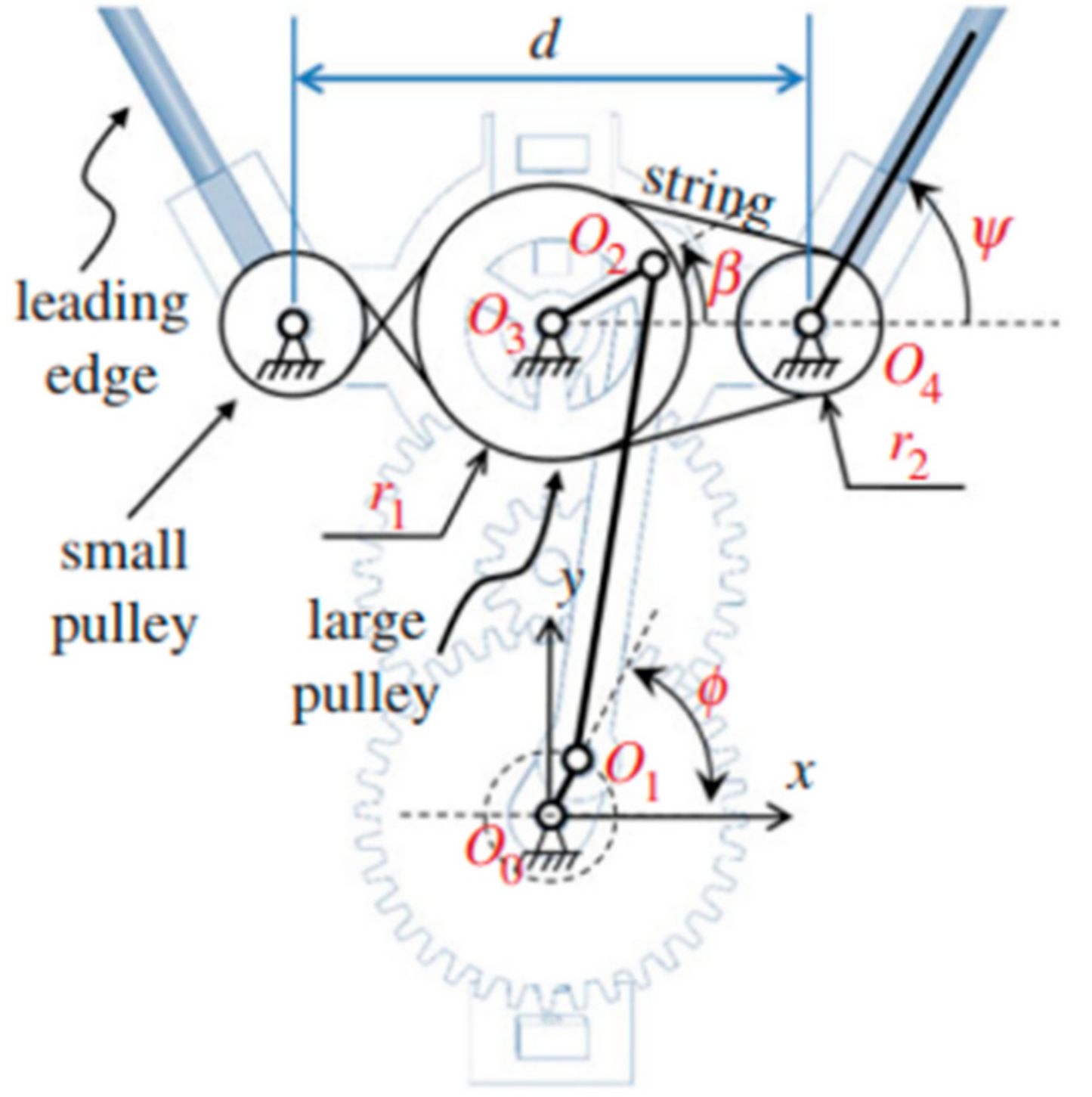
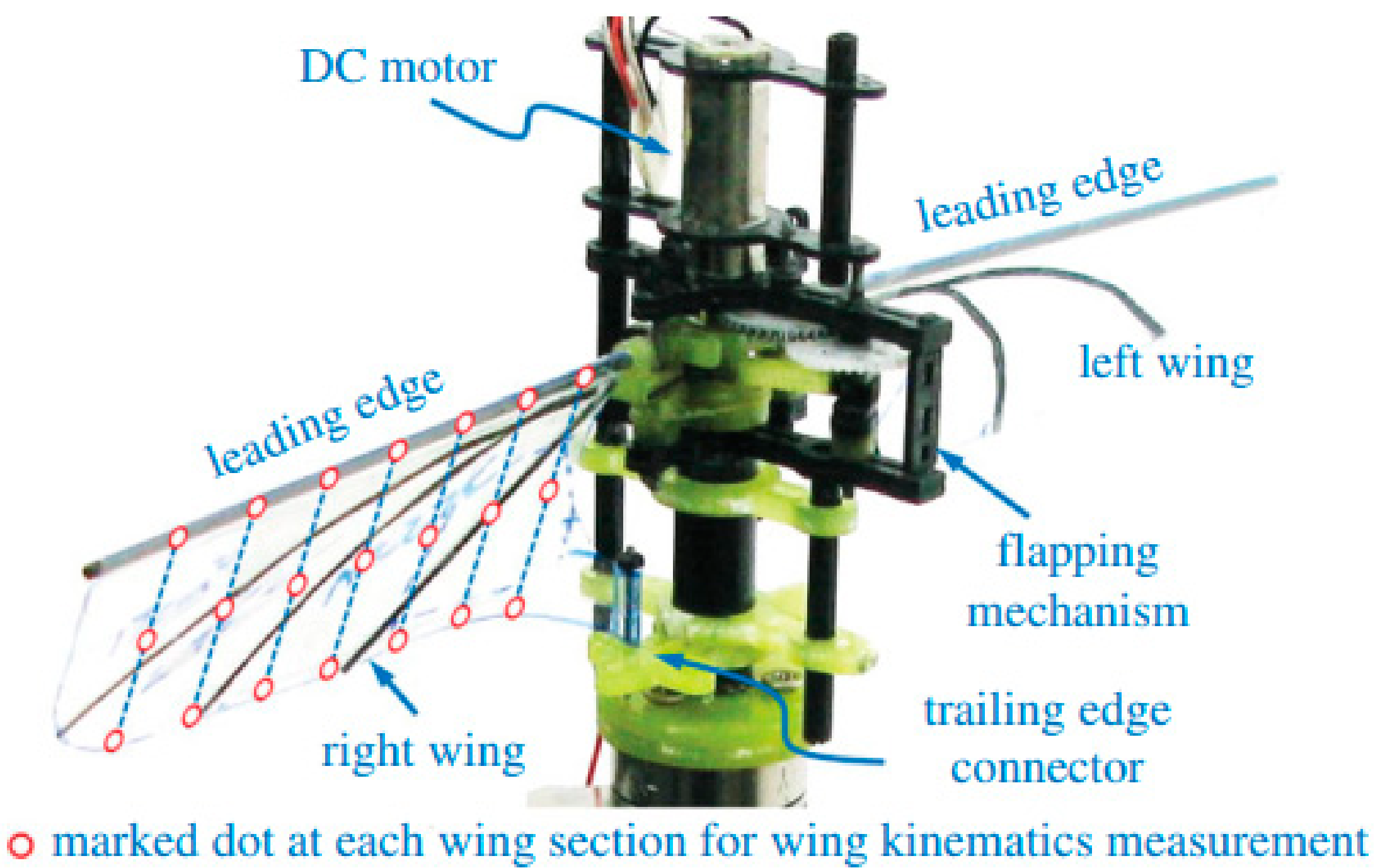
2.1. Flapping Mechanism

Because the flapping mechanisms were described in detail in previous work [42], we just briefly explain them here. As shown in Figure 2, the flapping system in KU-Beetle includes four-bar linkage and pulley-string mechanisms. As shown in Figure 3a, this combination enables a large flapping amplitude (Ψ) of more than 180°, allowing the wing pair to press close to each other at each half stroke and thus taking advantage of the clap-and-fling effect. The strength of the clap-and-fling effect depends on wing distance—the distance between two wings’ pivot points, denoted by d. As in previous work, two wing distances were investigated: 16 mm (0.64c_m) in which the clap-and-fling effect was strong, and 40 mm (1.6c_m) in which the clap-and-fling effect was almost diminished (Figure 3).

The wing veins were made of carbon strips and the wing membranes were made of polyethylene terephthalate (Figure 4). The wing length from the root to tip (R) was 70 mm. The mean chord (cm) was 25 mm. Each wing’s membrane rotates around a carbon rod attached at the leading edge. The trailing edge at the wing root was connected to the trailing edge connector. These configurations allow the wings to perform span-wise twist and chord-wise camber during the flapping motion.

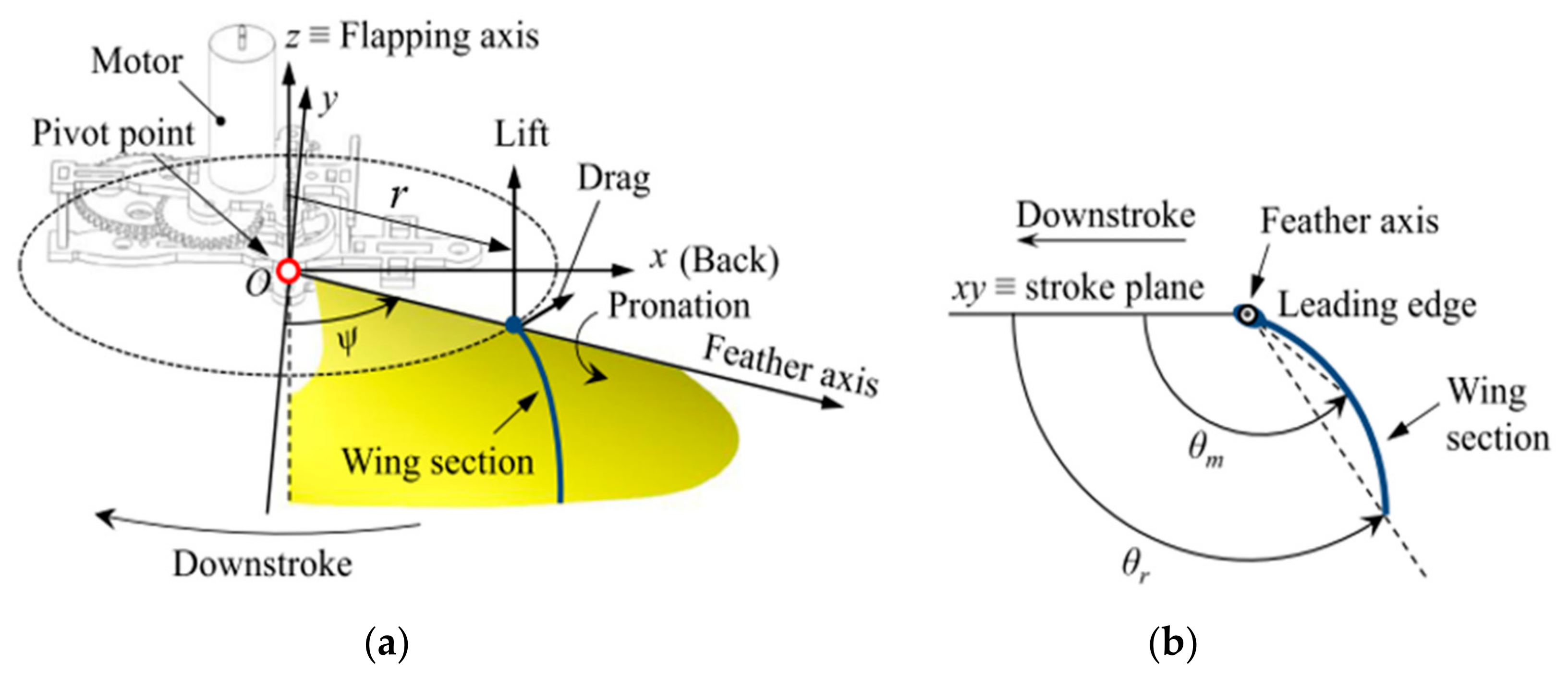
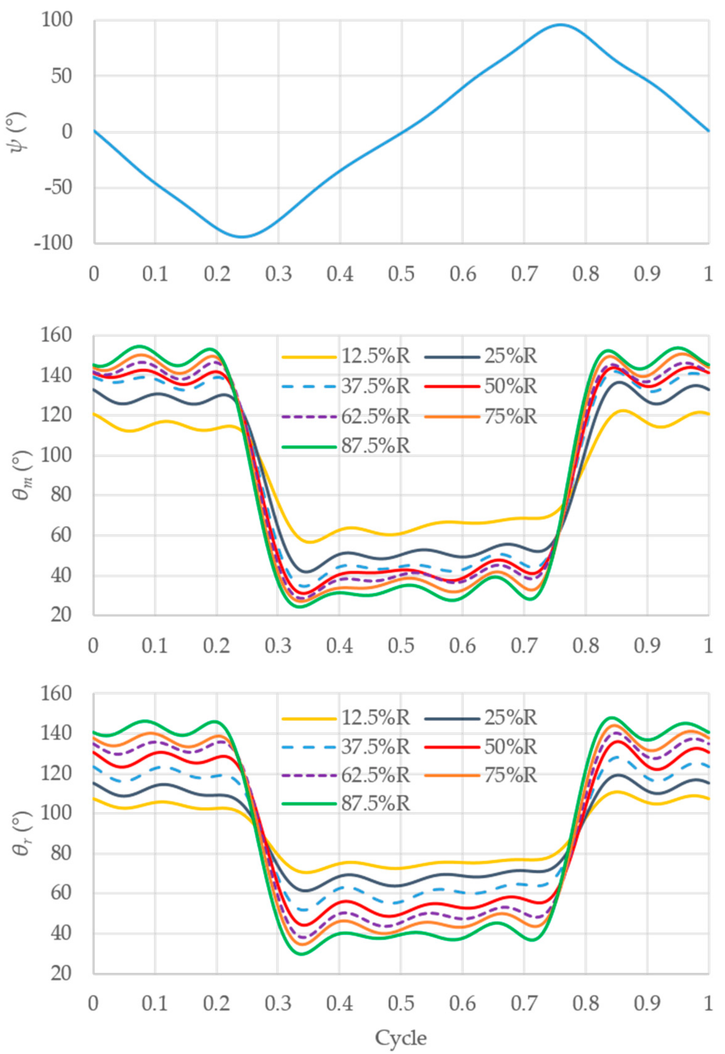
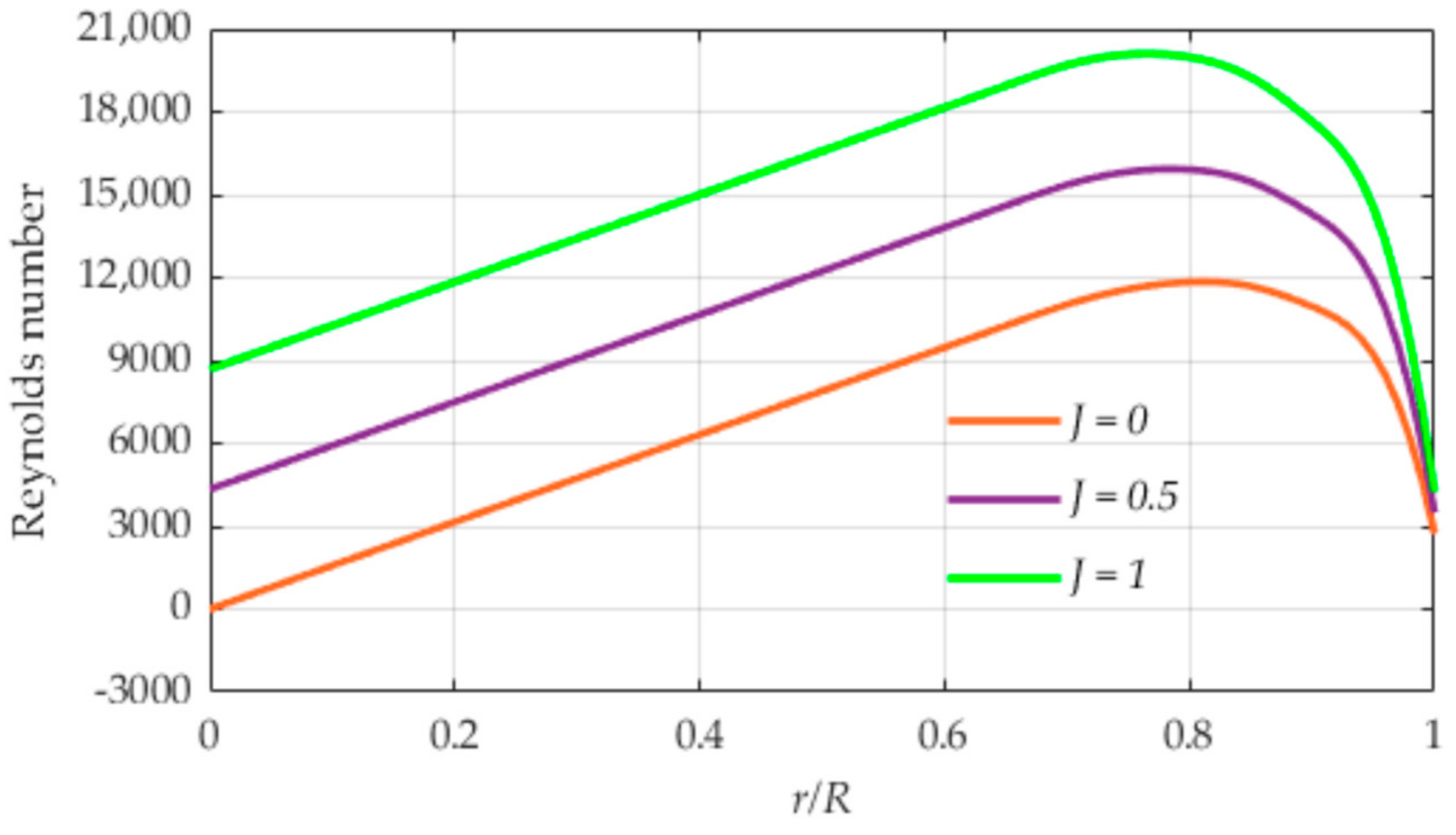
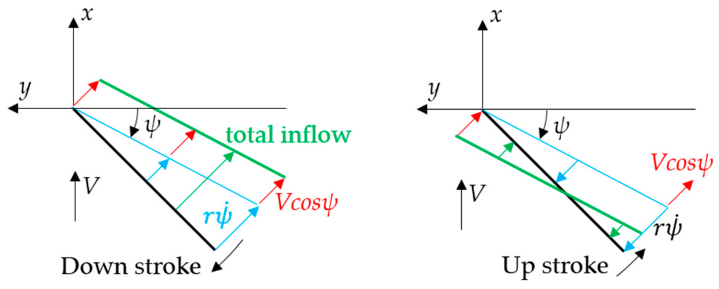
2.2. Wing Kinematics

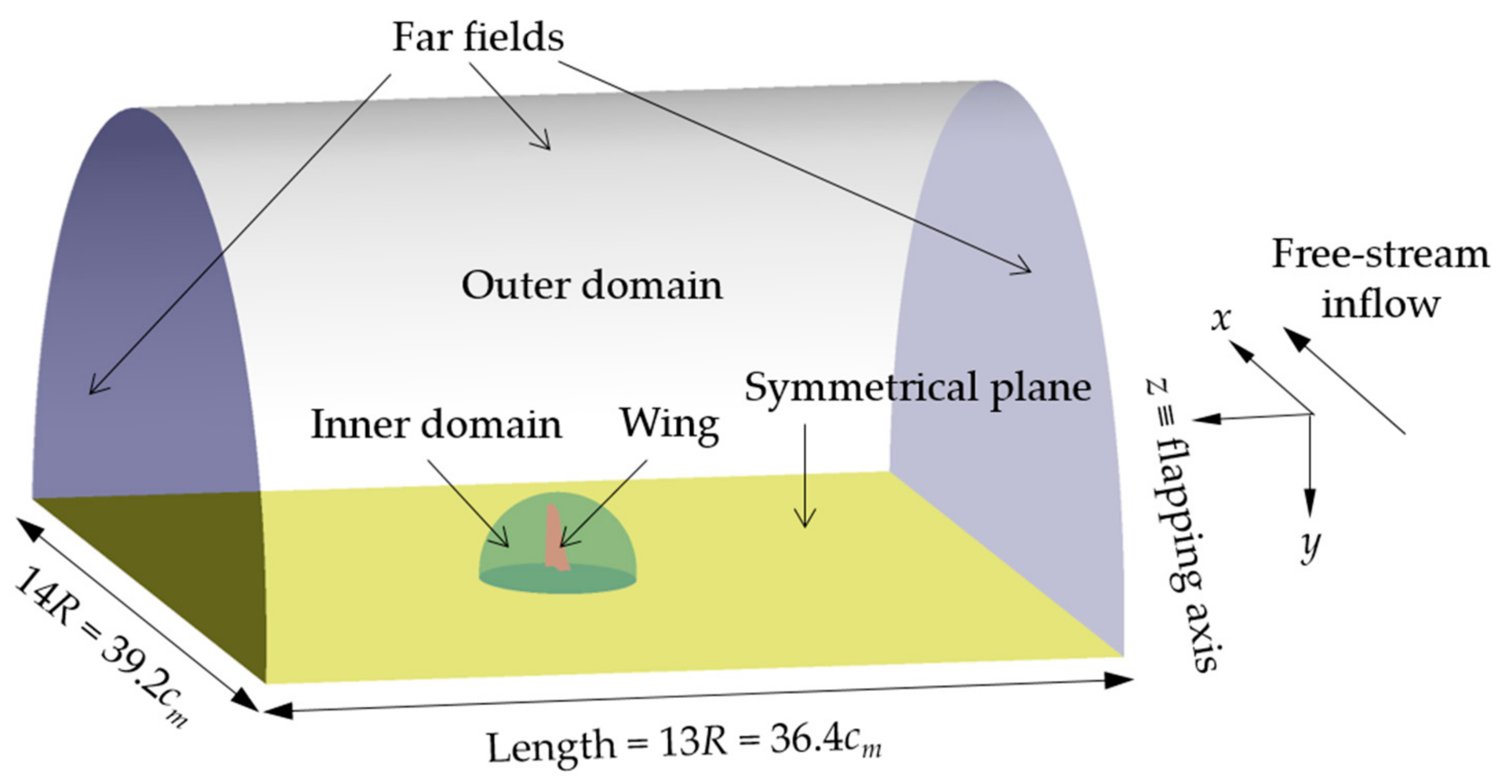
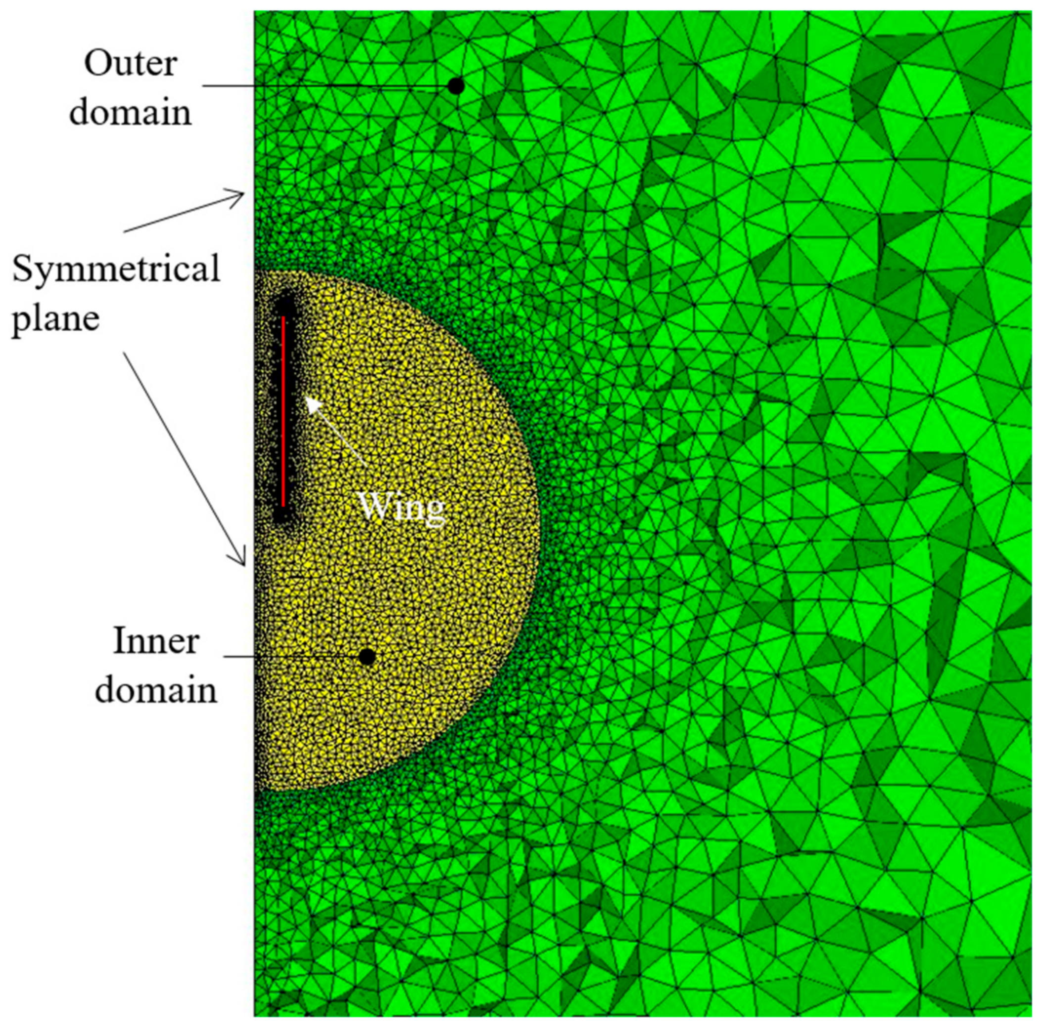
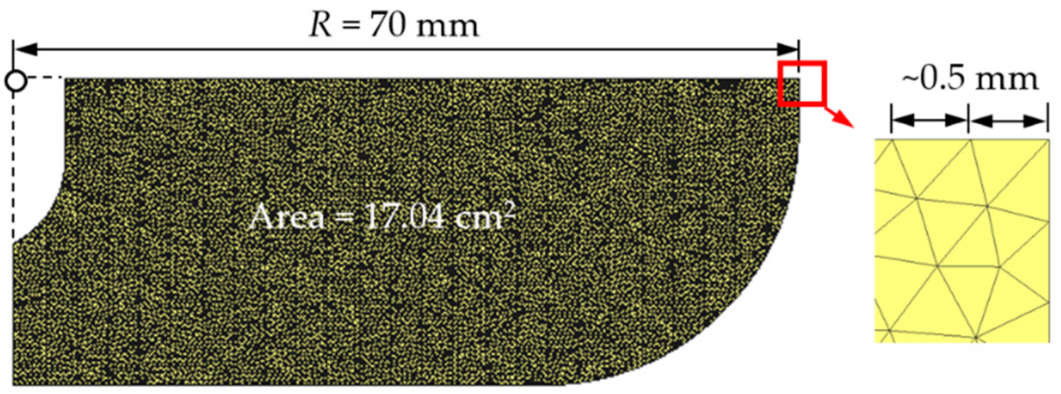
The parameters defining the wing kinematics were explained in Ref. [44]. The wing pitches around a feather axis which instantaneously revolves around a flapping axis (Figure 5a). In KU-Beetle, the feather axis is located at the leading edge of the wing. The flapping angle (ψ) between the feather axis and the mid-stroke plane—the plane perpendicular to the longitudinal symmetrical plane of the FW-MAV—determines the position of the feather axis. The camber of each wing section was modeled as a parabolic curve. Its orientation and shape were determined by two parameters: the mid-chord angle (θ_m) and the full-chord angle (θ_r) (Figure 5b). In order to measure ψ, θ_m and θ_r for various span-wise positions, the three-dimensional wing motion of KU-Beetle was captured using three synchronized hi-speed cameras. Then, the measured data was fitted by sum of sinusoidal functions. These processes were detailed in Refs. [42,45,46]. The time-courses of ψ, θ_m and θ_r are shown in Figure 6.

2.3. CFD Model

The CFD model was computed by the commercial software of ANSYS Fluent 16.2. Similar modelling technique as in Ref. [42], which was proven to provide converged solutions [46,47], was employed. Due to symmetry between the left and right wings, the CFD model was built for only left wing. Hence, the computational domain was a half cylinder whose length and diameter were of 13 and 14 times the wing length (36.4c_m and 39.2c_m), respectively. The symmetrical plane modeled the longitudinal mid-plane of the FW-MAV. With “symmetry” boundary type assigned to the plane, the wing–wing interaction between the left and right wings can be simulated. A significant difference from the previous work is that in this work, the volume inside the computational domain was divided into two parts: the inner domain containing the wing and the outer domain (Figure 7). The radius of the inner domain was 1.16 times the wing length.

In order to simulate the flapping motion, the mesh nodes on the wing must be updated at each time step using a user-defined function—a dynamic mesh feature in ANSYS Fluent. Consequently, the volume mesh must be remeshed. As shown in Figure 8, the volume mesh in the inner domain, which is directly attached to the wing, is much finer than the outer domain. In other words, it is of a high-density region. With the existence of the inner domain, the remeshing process focuses mainly on the elements in this domain, providing two benefits. First, the size of 3-D elements in the high-density region can be maintained during the remeshing process without remarkably increasing the number of elements. Second, the remeshing time is reduced, leading to a shorter computational time per time step.

The meshes were made by the commercial software ANSYS ICEM CFD 16.2. We used triangular elements for the surface mesh, and tetrahedral elements for the volume mesh. The wing was treated as a membrane whose surface was meshed into 21,000 triangles. The maximum edge length of each element was 0.5 mm (2% of c_m), as shown in Figure 9. The volume mesh was made from about 3 million tetrahedrons. The mesh was finest around the wing and became coarser toward the far field, inlet and outlet. In the high-density region (the inner domain in Figure 8), the minimum edge length was 0.5 mm at the cell layer attached to the wing, and the maximum was 2.5 mm toward the boundary of the region. The tetra growth rate away from the high density region was 1.1.

At far fields, the air flow velocity was set as free-stream condition. Note that the free-stream inflow is in horizontal direction from front to back of the FW-MAV, i.e., it aligns with the x-axis. Regarding the solution method, the pressure-based Semi-Implicit Method for Pressure-Link Equations (SIMPLE) algorithm was employed to solve the Navier–Stokes equations. The spatial discretization and transient formulation were set to second order. The time increment was 1/1600 the flapping cycle. For each time step, the residuals for equations on momentum and continuity were 10⁻⁴.

At each span-wise position r, the Reynolds number was computed as (V_m + V)c/ν where V_m = 2 Ψ fr is the average speed of the wing section at the position r, Ψ is the flapping amplitude (190°), f is the flapping frequency (20 Hz), V is the free-stream inflow speed, c is the local chord length, and ν is the kinematic viscosity of air (15.7 × 10⁻⁶ m²/s). We considered three inflow speeds: 0, 2.52 and 5.04 m/s, corresponding to advance ratios of 0, 0.5 and 1, respectively. The advance ratio (J) was computed as J = V/(2ΨfR_m), where R_m is the radius of the second moment of inertia of the wing (0.038 m). Variations of the Reynolds number from the wing root to tip for the three free-stream inflow speeds are plotted in Figure 10. For r from 0 to about 0.8R, because the velocity V_m—which is proportional to r—increases, the Reynolds number increases. However, for r from 0.8R to tip, because the local chord length decreases, the Reynolds number decreases. The maximum Reynolds numbers—occurring at around 80% wing length—were approximately 12,000 for hovering, 16,000 for J = 0.5 and 20,000 for J = 1. Since the maximum Reynolds numbers for all cases were in order of magnitude of 10⁴, the laminar model was chosen to simulate the flow.

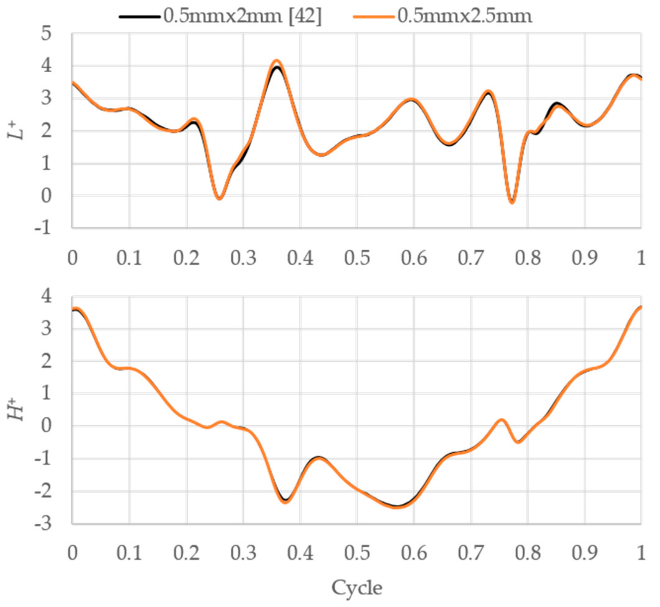
2.4. Grid-Independence Test and Validation

The grid-independence test with the same wing was reported in Ref. [47]. The grid size of the CFD model was determined by the element sizes on the wing surface (s₁) and in the high-density region (s₂). In Ref. [47], three grids corresponding to three sets of s₁ and s₂, namely, grid 1 (1 mm × 4 mm), grid 2 (0.75 mm × 3 mm), and grid 3 (0.5 mm × 2 mm) were tested. The aerodynamic forces at hovering were computed using the three grids. The former work shows that except for the slight differences in the force peaks, the time courses computed from the three grids were almost the same. Therefore, grid 1 could be considered grid independent. In the current work, we used the set of 0.5 mm × 2.5 mm which resulted in a finer mesh than grid 2. Moreover, the computational domain’s size of the current CFD model was also larger than that of the former work. Therefore, the current mesh could provide a converged solution. The time courses of the non-dimensional lift (L⁺) and horizontal force (H⁺) at hovering from the current mesh and from the grid 3—the finest mesh—are shown in Figure 11. The lift was in z-axis, i.e., normal to the stroke plane, and the horizontal force was in x-axis (see Figure 5a for the coordinate system). All forces were made non-dimensional by the reference force F_ref = ρ(2ΨfR_m)²S, where ρ is the air density (1.225 kg/m³), and S is the area of one wing (0.0017 m²). Hence, L⁺ = L/F_ref and H⁺ = H/F_ref where the superscript “⁺” indicates a non-dimensional quantity. As shown in Figure 11, except for slight differences in peaks of lift, the time courses for the two meshes were almost the same.

Note that the plots corresponding to grid 3 were extracted from the previous work [42], in which the effect of clap-and-fling at hovering were studied with the same wing and same wing kinematics, and the computational domain in that work was not divided into inner and outer domains. Grid 3 was the finest mesh among the three tested grid and it was proven to provide a reasonable estimation of the aerodynamic forces produced by the FW-MAV. A comparison to the experimental treatment showed that the mean lifts obtained from grid 3 of the previous CFD model for the two wing distances of 16 mm and 40 mm were, respectively, 3.2% and 7.5% larger than those measured by a dynamic load cell [42]. For the current CFD model, the differences were about 2.0% and 7.8%, as shown in

Table 1. Comparison between the previous and current CFD models.

CFD Model	Grid	CD 1			L+, 16 mm	L+, 40 mm
		Divided	Length	Diameter
Previous [42]	0.5 mm × 2 mm	no	33.6cm	33.6cm	2.27 (3.2%)	2.04 (7.5%)
Current	0.5 mm × 2.5 mm	yes	36.4cm	39.2cm	2.24 (2.0%)	2.04 (7.8%)

¹ CD is abbreviation for “computational domain”. The measured values of L⁺ extracted from Ref. [42] for wing distances of 16 mm and 40 mm were 2.20 and 1.89, respectively.

.

3. Results

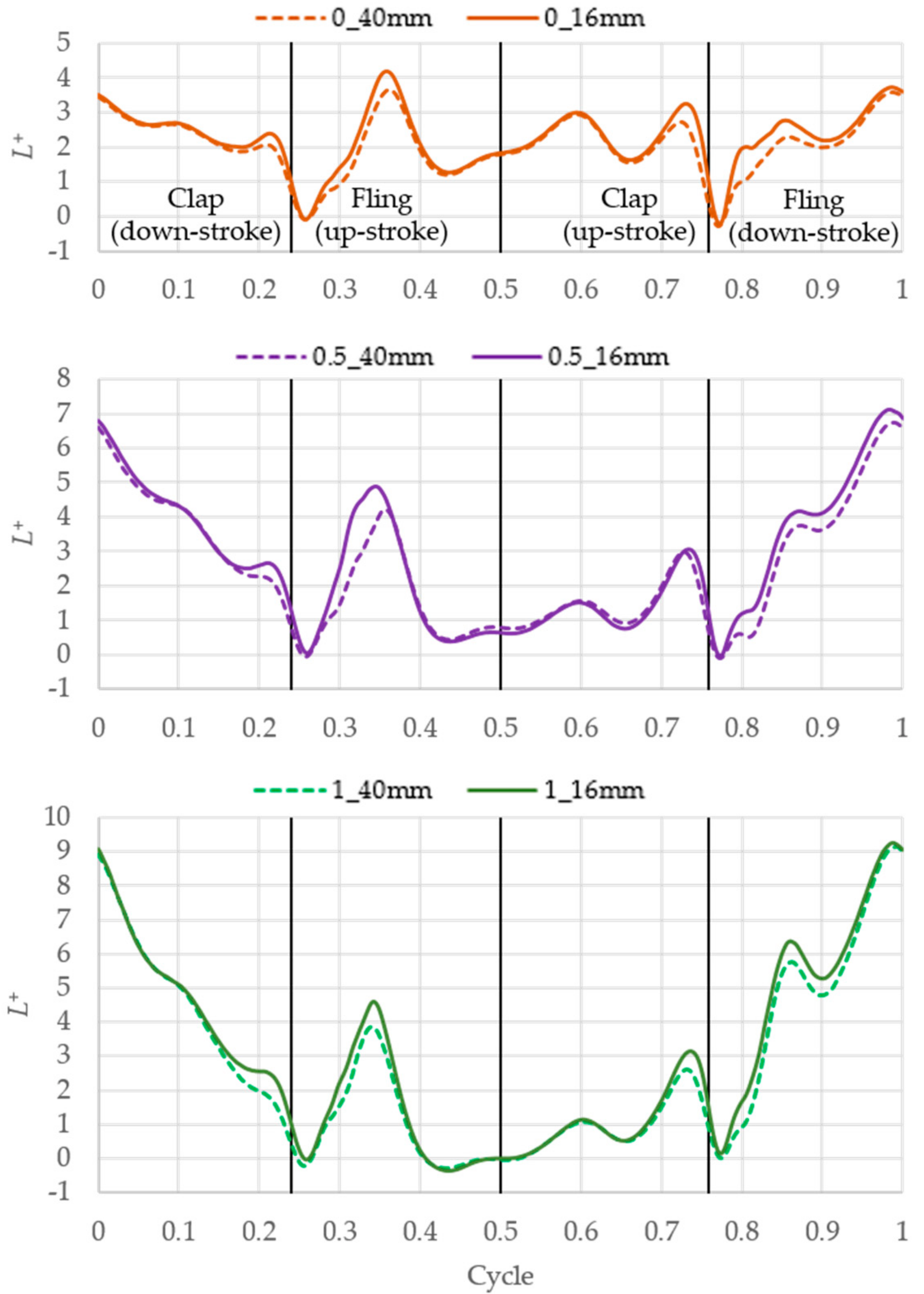
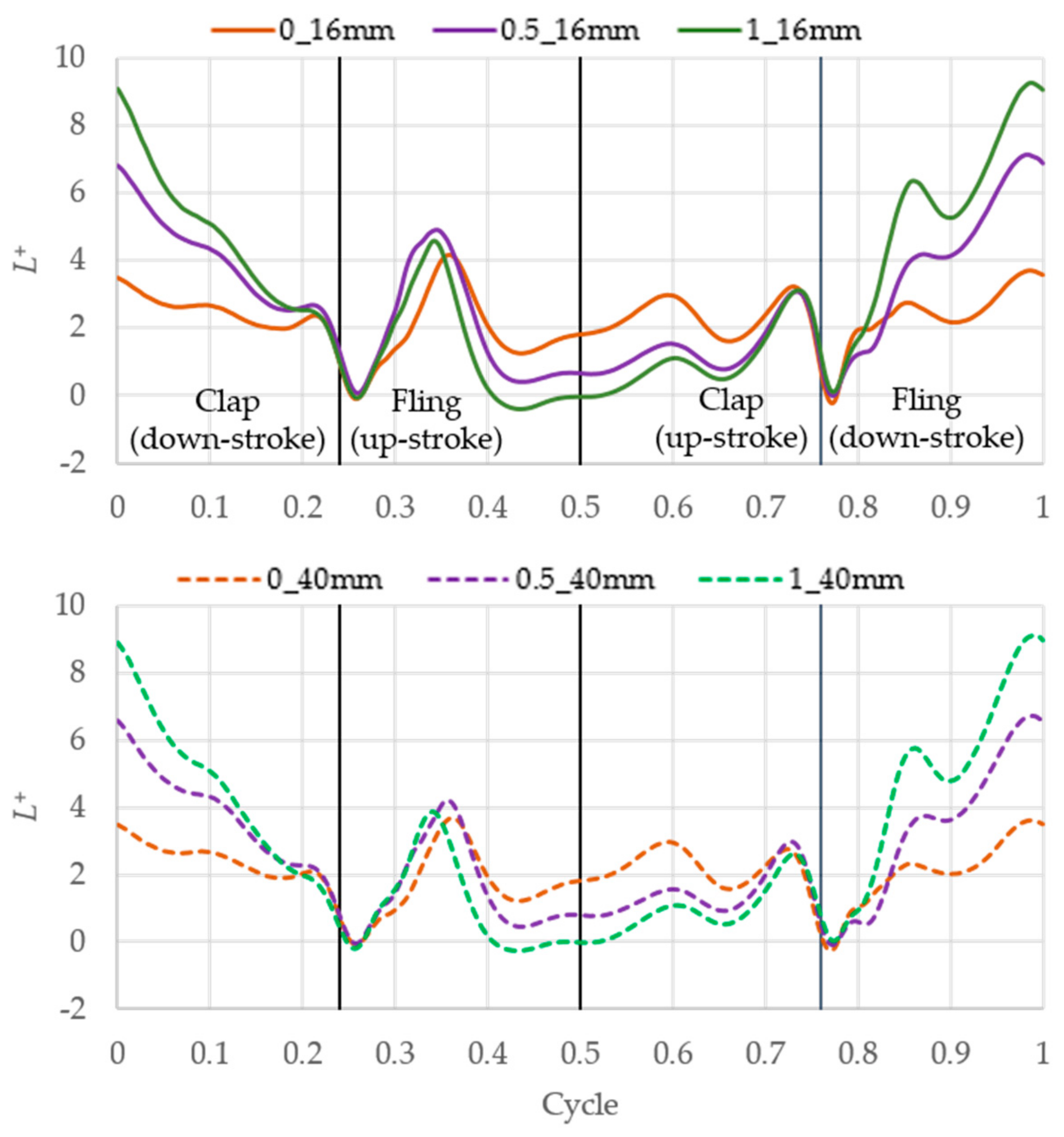
3.1. Effect of Clap-and-Fling on Lift Generation in Various Horizontal Free-Stream Inflow Speeds

All courses of lift, torque, and power consumption were taken at the third cycle when the flow became settled and the time courses became periodic. The time courses of lifts corresponding to various horizontal free-stream inflows are shown in Figure 12. The legend of each case is composed of two numbers connected by an underscore (_). The first number is the advance ratio. The second is the wing distance. For example, the legend 0.5_16 mm means that the advance ratio is 0.5 and the wing distance is 16 mm.

Let us define the non-dimensional time as t⁺ = t/T, where T is the flapping cycle. Each time course starts at the middle of the down stroke, divided into four phases: down-stroke clap, up-stroke fling, up-stroke clap, and down-stroke fling. These phases correspond to the second half of the down stroke (t⁺ = 0–0.241), the first half of the up stroke (t⁺ = 0.241–0.5), the second half of the up stroke (t⁺ = 0.5–0.759), and the first half of the down stroke (t⁺ = 0.759–1).

For all inflow speeds, there are lift augmentations in the case of 16 mm compared to the case of 40 mm, where the clap-and-fling effect is almost diminished due to far wing distance. The periods of lift augmentation in fling phases are longer than those in clap phases. Although the clap-and-fling effect is expected to increase the force, there are slight lift reductions near the middle of the up stroke for non-zero inflow cases.

The non-dimensional lifts are rearranged in two groups corresponding to two wing distances and plotted in Figure 13. The total inflow to a wing is the combination of the free-stream inflow and the inflow due to flapping motion (Figure 14). The free-stream inflow augments the total inflow during the down stroke and reduces it during the up stroke. As a result, when J increases from 0 to 1, the lifts in down-stroke phases increase while those in up-stroke phases decrease. Moreover, the contribution of the free-stream inflow to the total inflow is proportional to the term cosψ, which means that the influence of the free-stream inflow is largest around the middle of strokes where the flapping angle ψ is 0 and cosψ equals to 1. This explains why the differences between time courses are largest around the middle of strokes. Because the increased amount in the down stroke is larger than the reduced amount in the up stroke, the average lift over a flapping cycle increases with the increment of the inflow speed. This trend is applicable for both cases of wing distance, and agrees well with previous study on insect flight in forward/backward disturbance [48].

The contribution of clap and fling phases to the enhancement of mean lift is shown in

Table 2. Contribution of clap and fling phases to the mean lift enhancement.

L+	J = 0				J = 0.5				J = 1
	40 mm	16 mm	Enhancement	Contribution	40 mm	16 mm	Enhancement	Contribution	40 mm	16 mm	Enhance	Contribution
Clap (down)	0.57	0.59	0.02 (1.1%)	11.2%	0.89	0.94	0.04 (1.7%)	18.6%	1.05	1.10	0.05 (1.9%)	20.6%
Fling (up)	0.43	0.48	0.06 (2.8%)	28.4%	0.40	0.48	0.08 (3.3%)	34.9%	0.25	0.31	0.06 (2.2%)	23.9%
Clap (up)	0.56	0.61	0.04 (2.1%)	21.2%	0.37	0.36	−0.01 (−0.5%)	−5.0%	0.25	0.28	0.03 (1.1%)	12.5%
Fling (down)	0.48	0.56	0.08 (3.9%)	39.2%	0.80	0.92	0.12 (4.8%)	51.4%	1.14	1.25	0.11 (3.9%)	43.0%
Total (cycle)	2.04	2.24	0.20 (9.9%)	100%	2.47	2.70	0.23 (9.4%)	100%	2.70	2.94	0.25 (9.1%)	100%

. The mean lift is the average lift taken over a flapping cycle:

$${\overline{L}}^{+}={\displaystyle \underset{0}{\overset{1}{\int }}{L}^{+}(t^{+})d{t}^{+}}.$$

(1)

The lifts accumulated in clap and fling phases are computed as:

$$\text{Down-stroke} \mathrm{clap}: L^{+}={\displaystyle \underset{0}{\overset{0.241}{\int }}{L}^{+}(t^{+})d{t}^{+}},$$

(2)

$$\text{Up-stroke} \mathrm{fling}: L^{+}={\displaystyle \underset{0.241}{\overset{0.5}{\int }}{L}^{+}(t^{+})d{t}^{+}},$$

(3)

$$\text{Up-stroke} \mathrm{clap}: L^{+}={\displaystyle \underset{0.5}{\overset{0.759}{\int }}{L}^{+}(t^{+})d{t}^{+}},$$

(4)

$$\text{Down-stroke} \mathrm{fling}: L^{+}={\displaystyle \underset{0.759}{\overset{1}{\int }}{L}^{+}(t^{+})d{t}^{+}}.$$

(5)

As a result, the mean lift is the sum of lifts in all flapping phases:

$${\overline{L}}^{+}={\displaystyle \sum _{\mathrm{phases}}{L}^{+}}.$$

(6)

For each phase, the percentage in the column “enhancement” is the lift enhancement in percentage of the mean lift in case of 40 mm wing distance:

$$\mathrm{Enhancement} (\%)=\frac{L_{16\mathrm{m}\mathrm{m}}^{+}-L_{40\mathrm{m}\mathrm{m}}^{+}}{{\overline{L}}_{40\mathrm{m}\mathrm{m}}^{+}}\times 100\%.$$

(7)

The contribution of each phase to the mean lift enhancement is computed as:

$$\mathrm{Contribution}=\frac{L_{16\mathrm{m}\mathrm{m}}^{+}-L_{40\mathrm{m}\mathrm{m}}^{+}}{{\overline{L}}_{16\mathrm{m}\mathrm{m}}^{+}-{\overline{L}}_{40\mathrm{m}\mathrm{m}}^{+}}\times 100\%.$$

(8)

Equations (1)–(8) can be applied for torque and aerodynamic power consumption presented in the following sections.

For all free-stream inflow speeds, the lift enhancements in fling phases are larger than those in clap phases. For J = 0, 0.5 and 1, the two fling phases contribute totally 67.6%, 86.3% and 66.9% to the total lift enhancement, respectively. These amounts are more than twice those of the two clap phases, which, respectively, are 32.4%, 13.7% and 33.1%. Furthermore, for all inflow speeds, the contribution of the down-stroke fling is higher than that of the up-stroke fling. This is reasonable because the magnitude of the flapping angle in the dorsal reversal (96.3°) is larger than that in the ventral reversal (94.2°), resulting in stronger clap-and-fling effect.

For both up- and down-stroke flings, the lift enhancement increases when J increases from 0 to 0.5, and decreases with a further increment of J from 0.5 to 1. For down-stroke clap, the lift enhancement increases when J increases. For up-stroke clap, the lift enhancement decreases significantly from 2.1% to −0.5% when J increases from 0 to 0.5, and increases from −0.5% to 1.1% when J increases from 0.5 to 1. Overall, the enhancement in mean lift over a flapping cycle slightly decreases from 9.9% at J = 0 to 9.4% at J = 0.5 and 9.1% at J = 1.

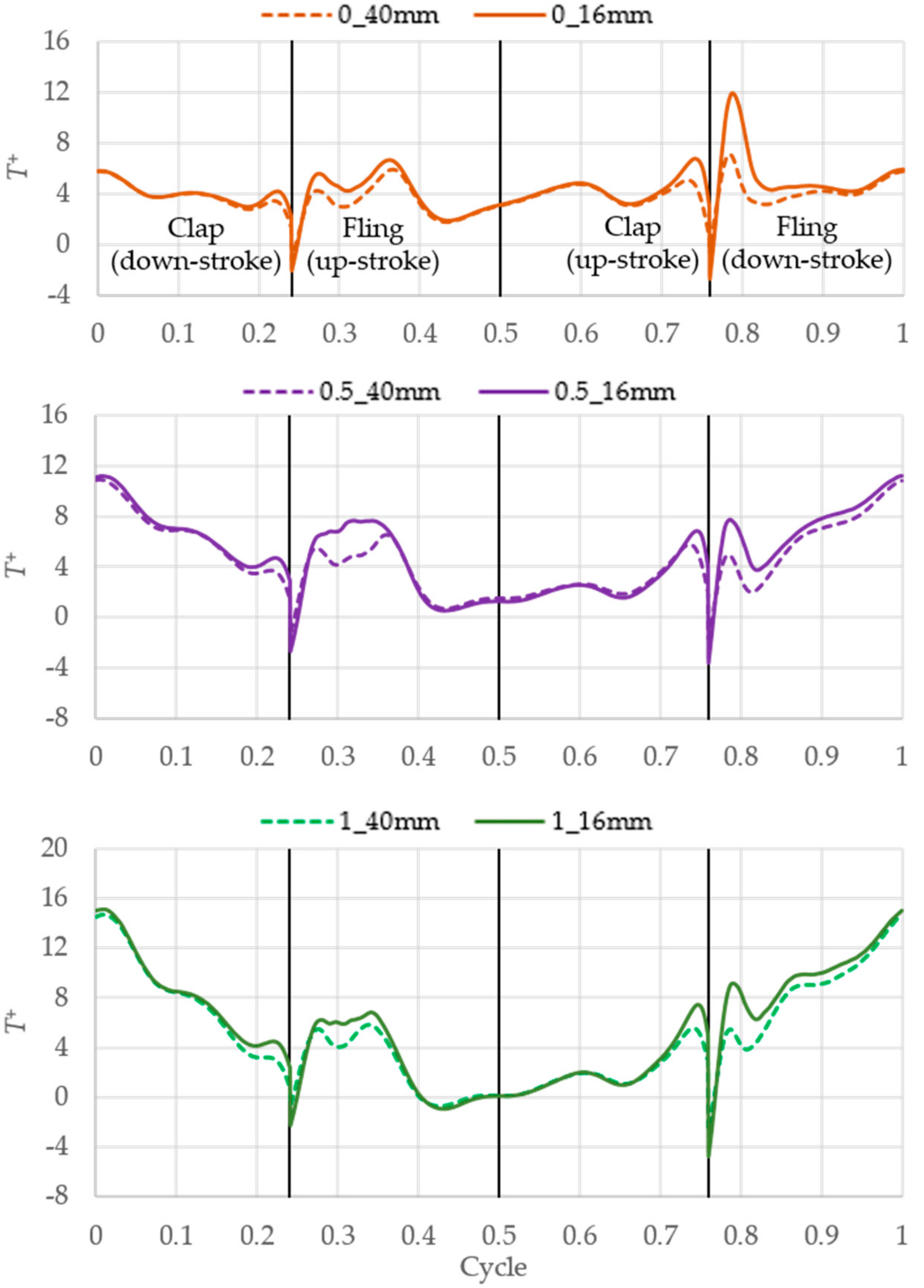
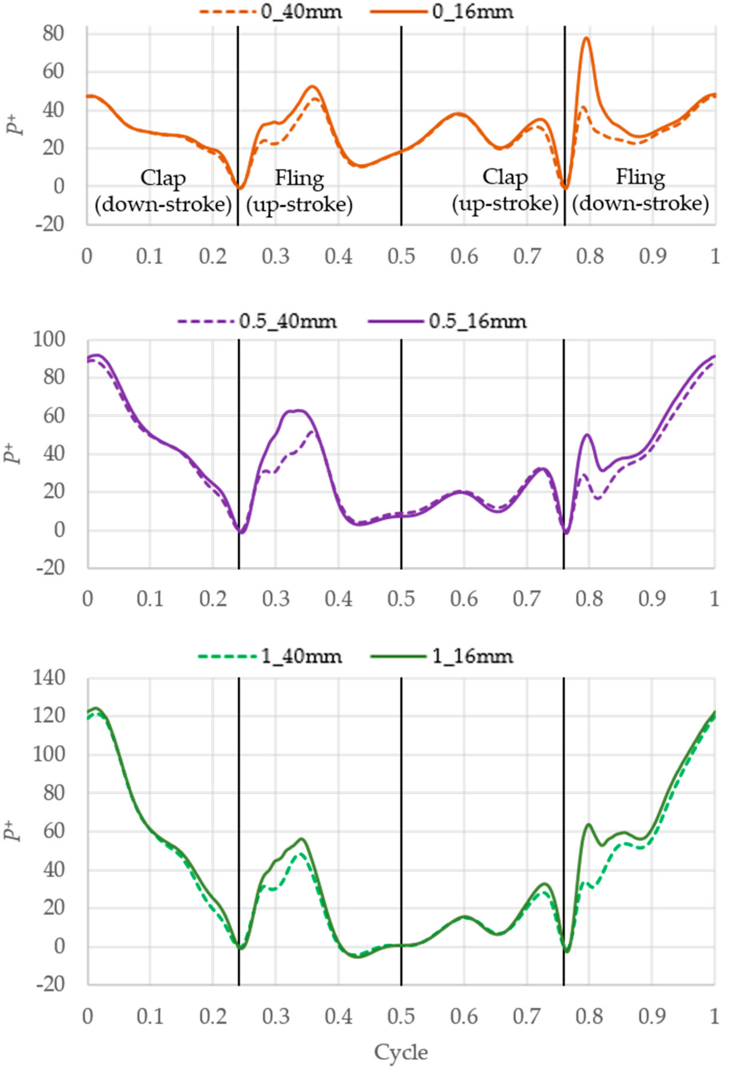
3.2. Effect of Clap-and-Fling on Torque and Aerodynamic Power Consumption

Torque (T) is the moment opposing the revolving motion of the wing. Let define M_z as the aerodynamic moment about the flapping axis (z-axis in Figure 5a). For the left wing, torque equals to M_z in the down stroke and −M_z in the up stroke. The aerodynamic power consumption is computed as P = −M_z$\dot{\psi }$, where $\dot{\psi }$ is the time derivative of the flapping angle ψ. The non-dimensional torque (T⁺) and power consumption (P⁺) were computed as T⁺ = T/(F_refc_m) and P⁺ = P/(F_refc_mf).

The time courses of torque and power consumption for various inflow speeds are plotted in Figure 15 and Figure 16, respectively. Similar to the lift, for all inflow speeds, there are increments in torque and power consumption in case of 16 mm compared to the case of 40 mm. The augmentations occur mainly during stroke reversal. The periods of augmentation in fling phases are longer than those in clap phases.

The contribution of clap and fling phases to the augmentations of the mean torque and power consumption are shown in

Table 3. Contribution of clap and fling phases to the mean torque enhancement.

T+	J = 0				J = 0.5				J = 1
	40 mm	16 mm	Enhancement	Contribution	40 mm	16 mm	Enhancement	Contribution	40 mm	16 mm	Enhancement	Contribution
Clap (down)	0.93	0.96	0.03 (0.9%)	6.5%	1.54	1.63	0.09 (2.1%)	19.5%	1.89	2.00	0.11 (2.2%)	20.5%
Fling (up)	0.85	0.99	0.13 (3.5%)	26.3%	0.84	0.98	0.14 (3.2%)	29.7%	0.60	0.69	0.09 (1.7%)	16.4%
Clap (up)	1.02	1.12	0.09 (2.4%)	18.1%	0.71	0.71	−0.01 (−0.1%)	−1.3%	0.52	0.58	0.06 (1.3%)	12.1%
Fling (down)	1.03	1.28	0.25 (6.5%)	49.1%	1.43	1.68	0.25 (5.5%)	52.1%	1.97	2.24	0.27 (5.4%)	51.1%
Cycle	3.83	4.34	0.51 (13.3%)	100%	4.52	5.00	0.48 (10.6%)	100%	4.98	5.50	0.52 (10.5%)	100%

and

Table 4. Contribution of clap and fling phases to the mean power consumption enhancement.

P+	J = 0				J = 0.5				J = 1
	40 mm	16 mm	Enhancement	Contribution	40 mm	16 mm	Enhancement	Contribution	40 mm	16 mm	Enhancement	Contribution
Clap (down)	6.7	6.8	0.11 (0.4%)	3.5%	11.4	12.0	0.53 (1.7%)	15.7%	14.4	14.9	0.55 (1.5%)	15.7%
Fling (up)	5.7	6.7	0.98 (3.7%)	30.2%	5.8	7.1	1.27 (3.9%)	37.3%	4.2	5.0	0.81 (2.2%)	23.0%
Clap (up)	6.8	7.2	0.36 (1.4%)	11.0%	4.5	4.2	−0.24 (−0.7%)	−7.0%	3.1	3.3	0.20 (0.6%)	5.8%
Fling (down)	7.2	9.0	1.80 (6.8%)	55.3%	10.5	12.3	1.83 (5.7%)	53.9%	14.6	16.5	1.96 (5.4%)	55.5%
Cycle	26.5	29.7	3.25 (12.3%)	100%	32.2	35.6	3.40 (10.5%)	100%	36.3	39.8	3.53 (9.7%)	100%

. For all inflow speeds, the total contributions of the fling phases are more than twice of the clap phases. When J increases from 0 to 0.5 and 1, the augmentation in torque due to clap-and-fling effect decreases from 13.3% to 10.6% and 10.5%. Meanwhile, the augmentation in power consumption decreases from 12.3% to 10.5% and 9.7%.

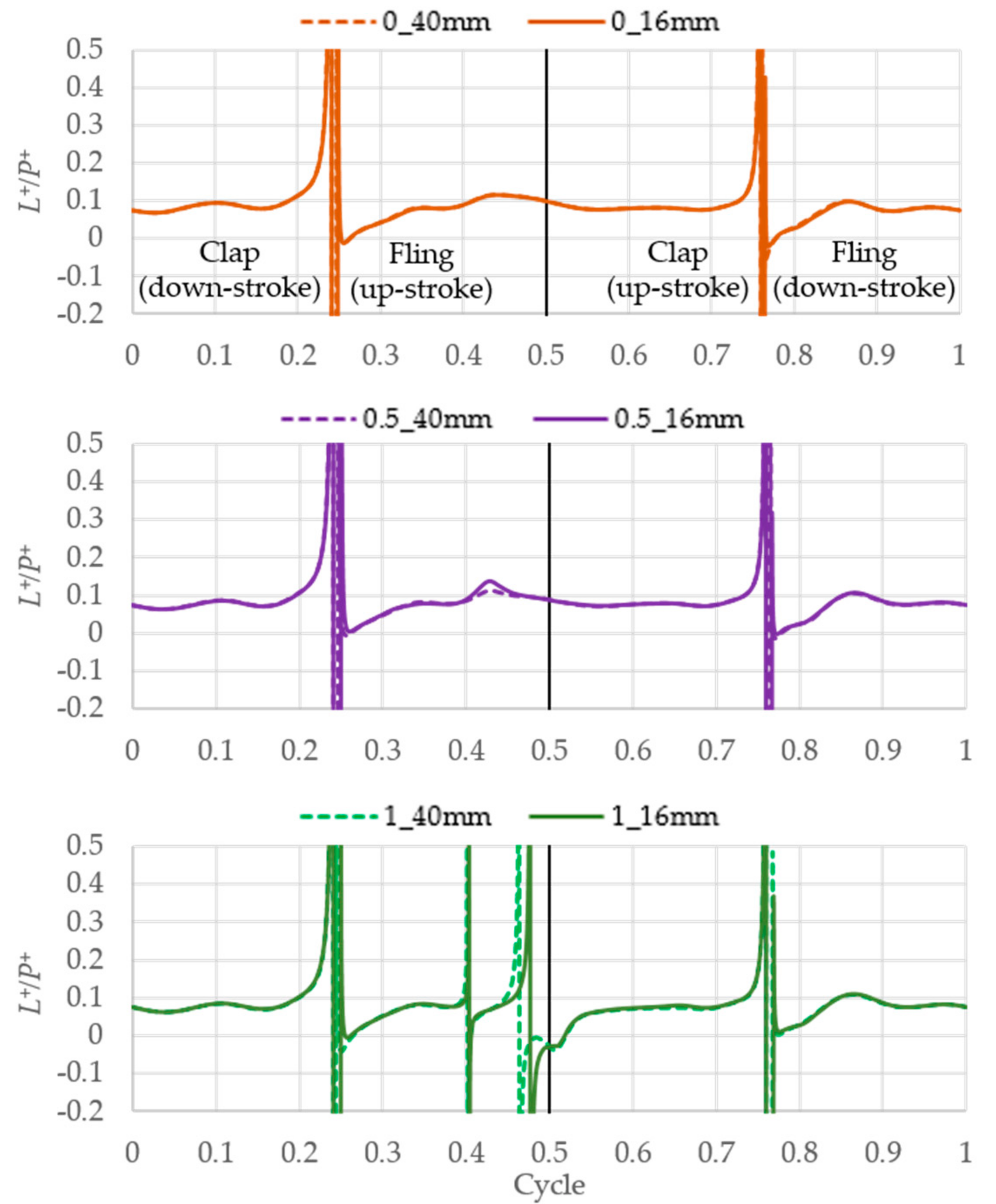
3.3. Effect of Clap-and-Fling on Aerodynamic Efficiency

In this work, the aerodynamic efficiency is represented by lift-to-power ratio (L⁺/P⁺). The time courses of L⁺/P⁺ are plotted in Figure 17. For all investigated inflow speeds, L⁺/P⁺ for the two wing distances are almost the same over the flapping cycle.

The lift-to-power ratios of all phases in the stroke cycle and the ratio between mean lift and mean power consumption are shown in

Table 5. Lift-to-power ratio of different phases and the ratio between mean lift and mean power consumption.

L+/P+ × 102	J = 0			J = 0.5			J = 1
	40 mm	16 mm	Enhancement	40 mm	16 mm	Enhancement	40 mm	16 mm	Enhancement
Clap (down)	8.53	8.72	0.19 (2.2%)	7.81	7.82	0.01 (0.1%)	7.32	7.38	0.07 (0.9%)
Fling (up)	7.43	7.20	−0.23 (−3.1%)	6.91	6.82	−0.10 (−1.4%)	6.04	6.23	0.19 (3.2%)
Clap (up)	8.23	8.42	0.19 (2.30%)	8.33	8.52	0.19 (2.32%)	8.02	8.46	0.43 (5.4%)
Fling (down)	6.68	6.23	−0.45 (−6.7%)	7.62	7.45	−0.17 (−2.2%)	7.85	7.56	−0.29 (−3.7%)
${\overline{L}}^{+}/{\overline{P}}^{+}\times {10}^2$	7.71	7.55	−0.16 (−2.1%)	7.66	7.58	−0.08 (−1.1%)	7.44	7.40	−0.04 (−0.6%)

. Note that the ratio between the mean lift and mean power consumption is not the sum of lift-to-power ratio of the four phases. This can be explained in following relationship:

$$\frac{{\overline{L}}^{+}}{{\overline{P}}^{+}}=\frac{{\displaystyle \sum _{\mathrm{phases}}{L}^{+}}}{{\displaystyle \sum _{\mathrm{phases}}{P}^{+}}}\ne {\displaystyle \sum _{\mathrm{phases}}\frac{L^{+}}{P^{+}}}.$$

(9)

Therefore, the “contribution” term presented in the previous tables is dismissed in Table 5. In addition, for each phase, the percentage in “enhancement” column of Table 5 is computed as:

$$\mathrm{enhancement}(\%)=\frac{L_{16\mathrm{m}\mathrm{m}}^{+}/P_{16\mathrm{m}\mathrm{m}}^{+}-L_{40\mathrm{m}\mathrm{m}}^{+}/P_{40\mathrm{m}\mathrm{m}}^{+}}{L_{40\mathrm{m}\mathrm{m}}^{+}/P_{40\mathrm{m}\mathrm{m}}^{+}}\times 100\%.$$

(10)

For all advance ratios, the clap phases in case of 16mm augment the lift-to-power ratio compared to the case of 40 mm. On the other hand, except for the up-stroke fling of J = 1, the fling phases reduce the lift-to-power ratio. Moreover, the free-stream inflow augments the enhancement of L⁺/P⁺ in up-stroke phases. When J increases from 0 to 0.5 and 1, the enhancement of L⁺/P⁺ due to up-stroke fling increases from −3.1% to −1.4% and 3.2%, while that due to up-stroke clap increases from 2.30% to 2.32% and 5.4%. With the same inflow speed, the mean lift to mean power ratio in case of 16mm is slightly reduced compared to the case of 40 mm. When the advance ratio increases from 0 to 0.5 and 1, the reduction amount decreases from 2.1% to 1.1% and 0.6%, respectively.

4. Discussion

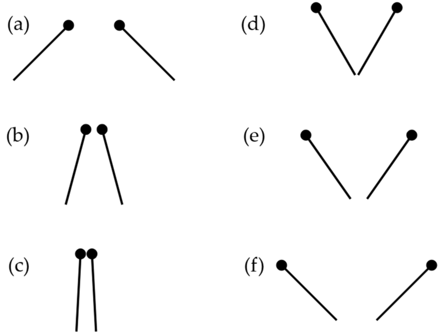
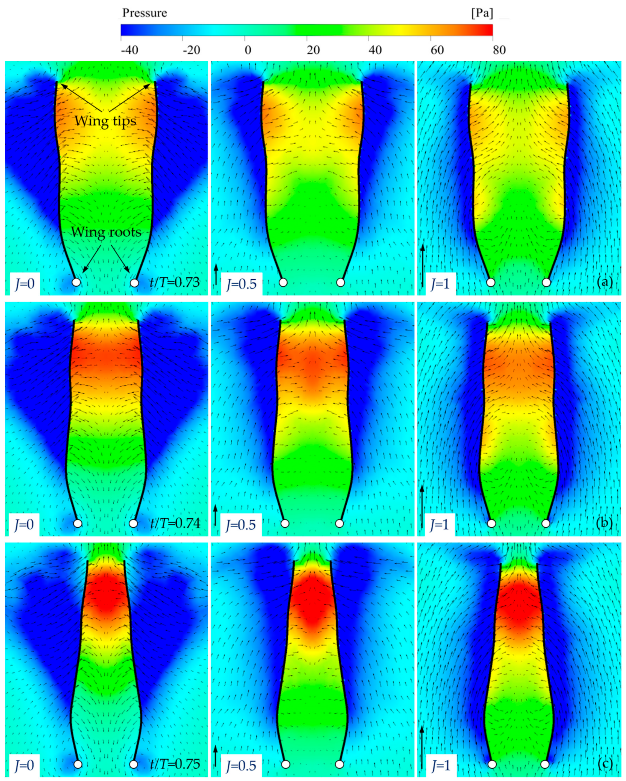
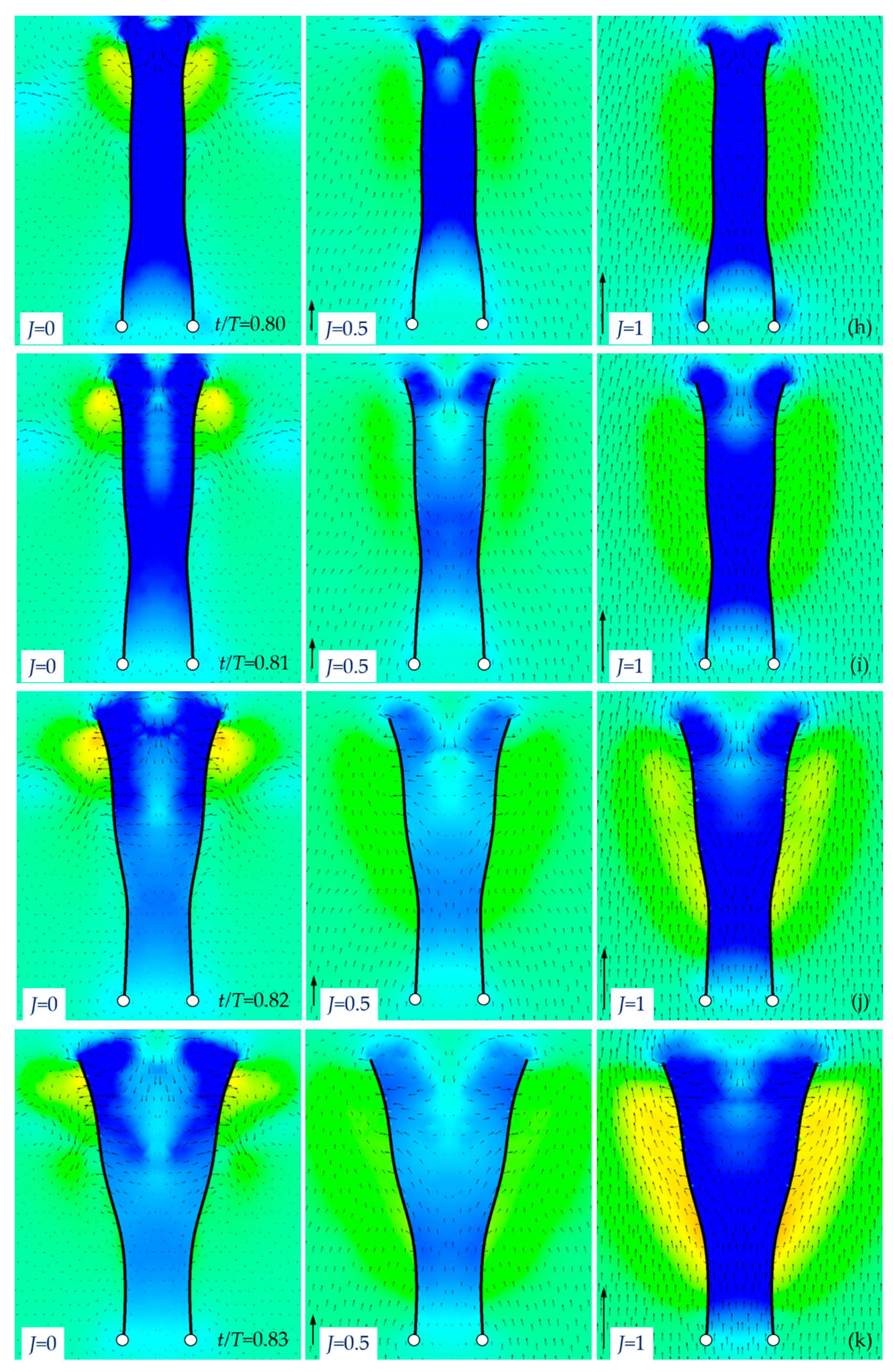
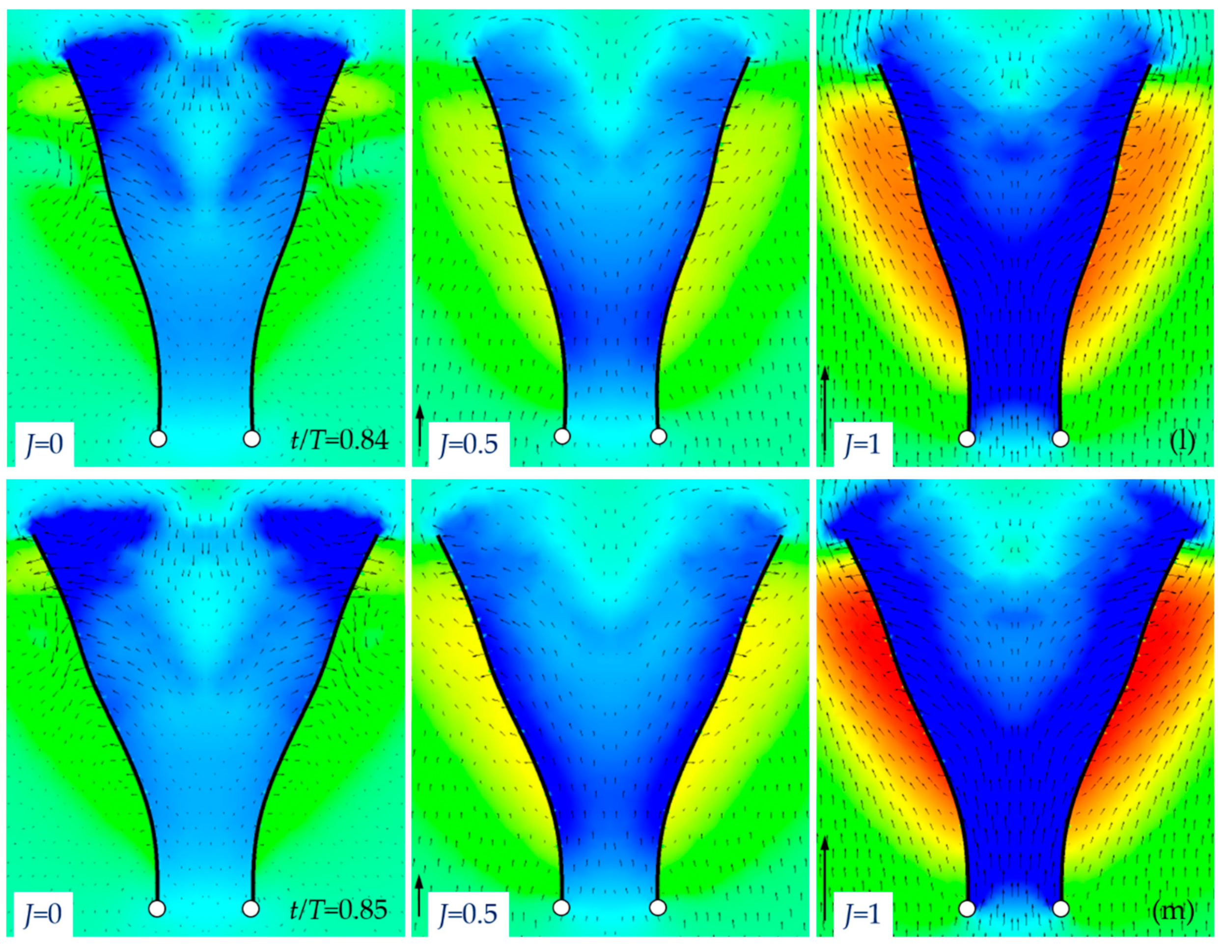
4.1. Force Augmentation Mechanism by Clap-and-Fling Effect

To explain why the force and torque trends observed in Section 3 occur, first, we investigated how the short wing distance—corresponding to a strong clap-and-fling effect—augments the force and torque generation. For this purpose, the pressure and flow velocity during the stroke reversal—the interval when the wing–wing interaction occurs—were examined. Because it is hard to interpret these flow fields in three-dimensional (3-D) view, the flow fields in 75%R-plane were plotted. As shown in Figure 18, the 75%R-plane is normal to the x-axis, located 75% wing length from the wing root (see Figure 5a for the coordinate system). As shown in Figure 3, the leading edges of the two wings are closest near the tip, implying that the clap-and-fling effect is strongest around this area. However, the clap-and-fling effect at the tip may be weak than the inner due to short local chord length. Therefore, the position of 75%R was chosen for the flow visualization.

The flow fields in 75%R-plane for J = 1 during down-stroke clap and up-stroke fling are plotted in Figure 19 and Figure 20. The flow fields for J = 0 and J = 0.5 show similar phenomena and can be found in Supplementary Materials. Right before the stroke reversal, the flapping speed is decelerated to 0 to prepare for the next stroke. In case of 40 mm wing distance, because of slow flapping speed, the force generation during the stroke reversal is low, manifested by the low-pressure region below the wings. Because flapping speed is decelerated, the pressure field below the wing pair becomes weaker when the time progresses to the end of the clap phase. Meanwhile, for the case of 16 mm, because the leading edges of the wing pair press close to each other, the air between them is trapped. The trapped air forms a high-pressure region between the wing pair, resulting in higher force generation compared to the case of 40 mm. While the pressure field below the wings in case of 40 mm becomes weaker as time progresses, the pressure field in case of 16 mm becomes stronger. This is because the space between the two wings becomes narrower, hence the trapped air tends to be more compressed. Moreover, due to inertia force resulted from wing mass, the wing camber changes from curve-up (Figure 19a,b) to curve-down (Figure 19c,d). Compared to rigid wings, this configuration is more effective in pushing the trapped air out of the high-density region via the open space between the trailing edges, resulting in a stronger down-ward flow and higher lift generation. Because the force enhancement in clap phase is mainly due to the trapped air between the two wings, it occurs in only a short time near the end of a stroke when the two wings approach, manifested by the short period of lift and torque augmentations prior to the stroke reversal shown in Figure 12 and Figure 15.

The flow fields in 75%R-plane during the up-stroke fling for J = 1 are plotted in Figure 20. During the fling phase, the leading edges move away while the trailing edges approach. In case of 16 mm, the fling motion implemented in camber wing effectively pushes down the trapped air between the wing pair, creating a strong down-ward flow below the wings and enhances the lift generation (Figure 20a–f). Moreover, the fling-open motion rapidly expands the volume between the wings, creating a low-pressure region between them. Because the leading edges separate before the trailing edges, the low pressure region appears firstly near the leading edges (Figure 20a–c), then gradually expands to the whole space between the wings (Figure 20d–h). The low-pressure region increases the net pressure between the upper and lower faces of the wings, resulting in augmentation of force and torque. Because the force augmentation in fling phase bases on two mechanisms: the pushed-down trapped air during the beginning of the phase, and the low-pressure region due to expanded air volume between the wings, the augmentation period in this phase is longer than that in clap phase. Consequently, the contribution in force enhancement of the fling phase is higher than that of the clap phase.

4.2. Influence of Free-Stream Inflow on Clap-and-Fling Effect

To explain the influence of the free-stream inflow on clap-and-fling effect, the flow field from the root to tip was observed. Because it is hard to interpret the pressure field in 3-D view, the flow field was plotted in 25%c_m-plane. As shown in Figure 21, 25%c_m-plane is the plane normal to the flapping axis (z-axis) and is located 25%c_m below the leading edge. Because the local chord length decreases toward the tip, a position far from the leading edges will cause a lost in information of the flow field near the tip. However, a choice which is too close to the leading edges may not fully reflect the trapped air between the wings. As a result, the 25%c_m-plane was chosen for flow visualization. The flow filed in 50%R-plane can be found in the Supplementary Materials.

The flow fields in 25%c_m-plane during down-stroke reversal for all investigated advance ratios are compared in Figure 22. As mentioned before, the force enhancement during clap phase is due to the high-pressure region between the wings, resulting from the trapped air when two wings press close to each other. In case of non-zero inflow, during down-stroke clap (Figure 22a–d), the free-stream inflow prevents the trapped air between the wings from moving out, further increasing the pressure between the wing. Consequently, the force enhancement during down-stroke clap in case of non-zero inflow is higher than that in case of hovering. When the advance ratio increases from J = 0 to 1, the amount of trapped air increases, hence the force enhancement of down-stroke clap phase also increases.

The flow fields during up-stroke fling are shown in Figure 22e–h. The force enhancement during fling phase results from two mechanisms: the pushed-down trapped air (trapped-air effect) and the low-pressure region due to expanded air volume between the wings (low-pressure-region effect). During up-stroke fling, the trapped air is pushed down, creating a strong down-ward flow below the wings. Because the amount of trapped air in case of non-zero inflow is larger than that in case of hovering, the amount of pushed-down trapped air is also larger, resulting in a higher reaction force on the wings, thus increasing the force enhancement. However, the inflow also augments the amount of air rushing in to occupy the low-pressure region between the wings, resulting in a higher pressure in the low-pressure region, thus reducing the force enhancement. When the advance ratio increases from J = 0 to 0.5, the amount of trapped air increases significantly, hence the increment of trapped-air effect is dominant compared to the decrement of low-pressure-region effect, and the force enhancement increases. Meanwhile, when J increases from 0.5 to 1, the decrement of low-pressure-region is dominant, hence the force enhancement decreases.

The flow fields during up-stroke reversal for all investigated inflows are shown in Figure 23. During up-stroke clap (Figure 23a–d), when the flapping angle ψ is less than 90° (Figure 23a,b), the free-stream inflow dissipates the trapped air between the wings, decreasing the force enhancement. However, when the flapping angle becomes larger than 90° (Figure 23c,d), because the wing tips are close to each other than the roots, the free-stream inflow increases the amount of trapped air, thus augmenting the force enhancement. When J increases from 0 to 0.5, the reduction in force enhancement when ψ < 90° is dominant, hence the force enhancement decreases. On the other hand, when J increases from 0.5 to 1, the augmentation in the force enhancement when ψ > 90° becomes dominant, hence the force enhancement increases compared to the case of J = 0.5. However, the force augmentation for J = 1 is still lower than that for hovering. This implies that the free-stream inflow is unfavorable to the up-stroke clap.

The flow fields during down-stroke fling are shown in Figure 23e–m. When the flapping angle ψ is larger than 90° (Figure 23e–h), the inflow increases the amount of air rushing in the low-pressure region, increasing the pressure of this region and thus decreasing the force enhancement. However, when ψ becomes larger than 90°, the inflow eventually decreases the pressure in the low-pressure region, thus increasing the force enhancement. As a result, the force enhancement during down-stroke fling in non-zero inflow is higher than that in hovering.

5. Conclusions

Using a computational fluid dynamic method to compute aerodynamic forces generated by flapping wings, we identified the influence of horizontal free-stream inflow on aerodynamic performance of clap-and-fling mechanism in a FW-MAV. The study shows that in terms of lift enhancement due to clap, the inflow is more favorable in the down stroke than in upstroke. For all investigated inflow speeds, the clap-and-fling effect augments the lift and power consumption, but reduces the lift-to-power ratio. The reduction in the lift-to-power ratio decreases when the advance ratio increases from 0 to 1. This implies that in terms of aerodynamic efficiency, the inflow benefits the clap-and-fling effect in KU-Beetle.

In order to solely study the influence of the free-stream inflow on clap-and-fling effect, the same wing kinematics in hovering was used. This manner is applicable for a hovering FW-MAV in gust or forward/backward-motion disturbances. However, in order to fly forward, the FW-MAV must change its wing kinematics. In that case, the aerodynamic performance depends on both forward flight speed and the wing kinematics. The aerodynamic performance of clap-and-fling mechanism in forward flight can be a direction for future study.

References

1. Shyy, W.; Berg, M.; Ljungqvist, D. Flapping and Flexible Wings for Biological and Micro Air Vehicles. Prog. Aerosp. Sci. 1999, 35, 455–505. [Google Scholar] [CrossRef]
2. Keennon, M.; Klingebiel, K.; Won, H. Development of the Nano Hummingbird: A Tailless Flapping Wing Micro Air Vehicle. In Proceedings of the 50th AIAA Aerospace Sciences Meeting, Nashville, TN, USA, 9–12 January 2012; American Institute of Aeronautics and Astronautics: Nashville, TN, USA, 2012. [Google Scholar]
3. Karásek, M.; Muijres, F.T.; De Wagter, C.; Remes, B.D.W.; de Croon, G.C.H.E. A Tailless Aerial Robotic Flapper Reveals that Flies Use Torque Coupling in Rapid Banked Turns. Science 2018, 361, 1089–1094. [Google Scholar] [CrossRef] [Green Version]
4. Roshanbin, A.; Altartouri, H.; Karásek, M.; Preumont, A. COLIBRI: A Hovering Flapping Twin-Wing Robot. Int. J. Micro Air Veh. 2017, 9, 270–282. [Google Scholar] [CrossRef] [Green Version]
5. Phan, H.V.; Kang, T.; Park, H.C. Design and Stable Flight of a 21 g Insect-like Tailless Flapping Wing Micro Air Vehicle with Angular Rates Feedback Control. Bioinspir. Biomim. 2017, 12, 17. [Google Scholar] [CrossRef] [PubMed]
6. Ma, K.Y.; Chirarattananon, P.; Fuller, S.B.; Wood, R.J. Controlled Flight of a Biologically Inspired, Insect-Scale Robot. Science 2013, 340, 603–607. [Google Scholar] [CrossRef] [PubMed] [Green Version]
7. Nguyen, Q.-V.; Chan, W.L. Development and Flight Performance of a Biologically-Inspired Tailless Flapping-Wing Micro Air Vehicle with Wing Stroke Plane Modulation. Bioinspir. Biomim. 2018, 14, 25. [Google Scholar] [CrossRef] [PubMed]
8. Fei, F.; Tu, Z.; Zhang, J.; Deng, X. Learning Extreme Hummingbird Maneuvers on Flapping Wing Robots. In Proceedings of the 2019 International Conference on Robotics and Automation (ICRA), Montreal, QC, Canada, 20–24 May 2019; pp. 109–115. [Google Scholar]
9. Ellington, C.P. The Aerodynamics of Hovering Insect Flight. I. The Quasi-Steady Analysis. Phil. Trans. R. Soc. Lond. B 1984, 305, 1–15. [Google Scholar]
10. Weis-Fogh, T. Quick Estimates of Flight Fitness in Hovering Animals, Including Novel Mechanisms for Lift Production. J. Exp. Biol. 1973, 59, 169–230. [Google Scholar] [CrossRef]
11. Lighthill, M.J. On the Weis-Fogh Mechanism of Lift Generation. J. Fluid Mech. 1973, 60, 1–17. [Google Scholar] [CrossRef]
12. Cooter, R.J.; Baker, P.S. Weis-Fogh Clap and Fling Mechanism in Locusta. Nature 1977, 269, 53–54. [Google Scholar] [CrossRef]
13. Bennett, L. Clap and Fling Aerodynamics—An Experimental Evaluation. J. Exp. Biol. 1977, 69, 261–272. [Google Scholar] [CrossRef]
14. Miller, L.A.; Peskin, C.S. A Computational Fluid Dynamics of ‘clap and Fling’ in the Smallest Insects. J. Exp. Biol. 2005, 208, 195–212. [Google Scholar] [CrossRef] [PubMed] [Green Version]
15. Miller, L.A.; Peskin, C.S. Flexible Clap and Fling in Tiny Insect Flight. J. Exp. Biol. 2009, 212, 3076–3090. [Google Scholar] [CrossRef] [PubMed] [Green Version]
16. Ellington, C.P. The Novel Aerodynamics of Insect Flight: Applications to Micro-Air Vehicles. J. Exp. Biol. 1999, 202, 3439–3448. [Google Scholar] [CrossRef] [PubMed]
17. Marden, J.H. Maximum Lift Production during Takeoff in Flying Animals. J. Exp. Biol. 1987, 130, 235–258. [Google Scholar] [CrossRef]
18. Maxworthy, T. Experiments on the Weis-Fogh Mechanism of Lift Generation by Insects in Hovering Flight Part 1. Dynamics of the ‘Fling’. J. Fluid Mech. 1979, 93, 47–63. [Google Scholar] [CrossRef]
19. Spedding, G.R.; Maxworthy, T. The Generation of Circulation and Lift in a Rigid Two-Dimensional Fling. J. Fluid Mech. 1986, 165, 247–272. [Google Scholar] [CrossRef]
20. Sun, M.; Yu, X. Flows around Two Airfoils Performing Fling and Subsequent Translation and Translation and Subsequent Clap. Acta Mech. Sin. 2003, 19, 103–117. [Google Scholar]
21. Lehmann, F.-O.; Sane, S.P.; Dickinson, M. The Aerodynamic Effects of Wing–Wing Interaction in Flapping Insect Wings. J. Exp. Biol. 2005, 208, 3075–3092. [Google Scholar] [CrossRef] [Green Version]
22. Ellington, C.P.; van den Berg, C.; Willmott, A.P.; Thomas, A.L.R. Leading-Edge Vortices in Insect Flight. Nature 1996, 384, 626–630. [Google Scholar] [CrossRef]
23. Dickinson, M.H.; Lehmann, F.-O.; Sane, S.P. Wing Rotation and the Aerodynamic Basis of Insect Flight. Science 1999, 284, 1954–1960. [Google Scholar] [CrossRef] [PubMed]
24. Birch, J.M.; Dickinson, M.H. Spanwise Flow and the Attachment of the Leading-Edge Vortex on Insect Wings. Nature 2001, 412, 729–733. [Google Scholar] [CrossRef]
25. Sane, S.P.; Dickinson, M.H. The Aerodynamic Effects of Wing Rotation and a Revised Quasi-Steady Model of Flapping Flight. J. Exp. Biol. 2002, 205, 1087–1096. [Google Scholar] [CrossRef] [PubMed]
26. Birch, J.M.; Dickinson, M.H. The Influence of Wing–Wake Interactions on the Production of Aerodynamic Forces in Flapping Flight. J. Exp. Biol. 2003, 206, 2257–2272. [Google Scholar] [CrossRef] [PubMed] [Green Version]
27. Vogel, S. Life in Moving Fluids: The Physical Biology of Flow, 2nd ed.; Princeton University Press: Princeton, NJ, USA, 1996. [Google Scholar]
28. Sane, S.P.; Dickinson, M.H. The Control of Flight Force by a Flapping Wing: Lift and Drag Production. J. Exp. Biol. 2001, 204, 2607–2626. [Google Scholar] [CrossRef]
29. Minotti, F.O. Unsteady Two-Dimensional Theory of a Flapping Wing. Phys. Rev. E 2002, 66, 10. [Google Scholar] [CrossRef]
30. Sane, S.P. The Aerodynamics of Insect Flight. J. Exp. Biol. 2003, 206, 4191–4208. [Google Scholar] [CrossRef] [Green Version]
31. Weis-Fogh, T. Unusual Mechanisms for the Generation of Lift in Flying Animals. Sci. Am. 1975, 233, 80–87. [Google Scholar] [CrossRef]
32. Ellington, C.P. Wing Mechanics and Take-Off Preparation of Thrips (Thysanoptera). J. Exp. Biol. 1980, 85, 129–136. [Google Scholar] [CrossRef]
33. Srygley, R.B.; Thomas, A.L.R. Unconventional Lift-Generating Mechanisms in Free-Flying Butterflies. Nature 2002, 420, 660–664. [Google Scholar] [CrossRef]
34. Ennos, A.R. The Kinematics and Aerodynamics of the Free Flight of Some Diptera. J. Exp. Biol. 1989, 142, 49–85. [Google Scholar] [CrossRef]
35. Götz, K.G. Course-Control, Metabolism and Wing Interference During Ultralong Tethered Flight in Drosophila Melanogaster. J. Exp. Biol. 1987, 128, 35–46. [Google Scholar] [CrossRef]
36. Brackenbury, J. Wing Kinematics during Natural Leaping in the Mantids Mantis Religiosa and Iris Oratoria. J. Zool. 1991, 223, 341–356. [Google Scholar] [CrossRef]
37. Ellington, C.P. The Aerodynamics of Hovering Insect Flight. III. Kinematics. Phil. Trans. R. Soc. Lond. B 1984, 305, 41–78. [Google Scholar]
38. Johansson, L.C.; Henningsson, P. Butterflies Fly Using Efficient Propulsive Clap Mechanism Owing to Flexible Wings. J. R. Soc. Interface 2021, 18, 10. [Google Scholar] [CrossRef]
39. Groen, M.; Bruggeman, B.; Remes, B.D.W.; Ruijsink, H.; van Oudheusden, B.; Bijl, H. Improving Flight Performance of the Flapping Wing MAV Delfly II. In Proceedings of the International Micro Air Vehicle Conference and Flight Competition, Braunschweig, Germany, 6–8 July 2010. [Google Scholar]
40. Zdunich, P.; Bilyk, D.; MacMaster, M.; Loewen, D.; DeLaurier, J.; Kornbluh, R.; Low, T.; Stanford, S.; Holeman, D. Development and Testing of the Mentor Flapping-Wing Micro Air Vehicle. J. Aircr. 2007, 44, 1701–1711. [Google Scholar] [CrossRef]
41. Nguyen, Q.-V.; Chan, W.L.; Debiasi, M. Design, Fabrication, and Performance Test of a Hovering-Based Flapping-Wing Micro Air Vehicle Capable of Sustained and Controlled Flight. In Proceedings of the International Micro Air Vehicle Conference and Competition (IMAV 2014), Delf, The Netherlands, 12–15 August 2014. [Google Scholar]
42. Phan, H.V.; Au, T.K.L.; Park, H.C. Clap-and-Fling Mechanism in a Hovering Insect-like Two-Winged Flapping-Wing Micro Air Vehicle. R. Soc. Open Sci. 2016, 3, 18. [Google Scholar] [CrossRef] [Green Version]
43. Nguyen, K.; Au, L.T.K.; Phan, H.-V.; Park, S.H.; Park, H.C. Effects of Wing Kinematics, Corrugation, and Clap-and-Fling on Aerodynamic Efficiency of a Hovering Insect-Inspired Flapping-Wing Micro Air Vehicle. Aerosp. Sci. Technol. 2021, 118, 11. [Google Scholar] [CrossRef]
44. Au, L.T.K.; Phan, H.V.; Park, S.H.; Park, H.C. Effect of Corrugation on the Aerodynamic Performance of Three-Dimensional Flapping Wings. Aerosp. Sci. Technol. 2020, 105, 11. [Google Scholar] [CrossRef]
45. Truong, T.Q.; Phan, V.H.; Park, H.C.; Ko, J.H. Effect of Wing Twisting on Aerodynamic Performance of Flapping Wing System. AIAA J. 2013, 51, 1612–1620. [Google Scholar] [CrossRef]
46. Au, L.T.K.; Phan, H.V.; Park, H.C. Comparison of Aerodynamic Forces and Moments Calculated by Three-Dimensional Unsteady Blade Element Theory and Computational Fluid Dynamics. J. Bionic Eng. 2017, 14, 746–758. [Google Scholar] [CrossRef]
47. Au, L.T.K.; Phan, V.H.; Park, H.C. Longitudinal Flight Dynamic Analysis on Vertical Takeoff of a Tailless Flapping-Wing Micro Air Vehicle. J. Bionic Eng. 2018, 15, 283–297. [Google Scholar] [CrossRef]
48. Xiong, Y.; Sun, M. Dynamic Flight Stability of a Bumblebee in Forward Flight. Acta Mech. Sin. 2008, 24, 25–36. [Google Scholar] [CrossRef]
Figure 1. Schematic of wing sections during “clap” (ac) and “fling” (df).
Aerospace 09 00108 g001
Figure 2. Scheme of the flapping mechanism in KU-Beetle. Reprinted from Ref. [42].
Aerospace 09 00108 g002
Figure 3. Composite images of the flapping wings at the end of up- and down-strokes. (a) The clap-and-fling effect is strong with wing distance of 16 mm (0.64cm); (b) The clap-and-fling effect is almost diminished with wing distance of 40 mm (1.6cm) Reprinted from Ref. [42].
Aerospace 09 00108 g003
Figure 4. Wing configuration. Reprinted from Ref. [42].
Aerospace 09 00108 g004
Figure 5. Definitions in the flapping-wing motion. (a) Feather axis, flapping axis, and flapping angle ψ; (b) The parabolic curve modeling camber of a wing section. Reprinted from Ref. [44].
Aerospace 09 00108 g005
Figure 6. The time courses of wing kinematics.
Aerospace 09 00108 g006
Figure 7. Computational domain.
Aerospace 09 00108 g007
Figure 8. Cross section of the computational domain.
Aerospace 09 00108 g008
Figure 9. Mesh on the wing surface. The white circle marks the pivot point.
Aerospace 09 00108 g009
Figure 10. Span-wise distribution of the Reynolds number for the three investigated inflow speeds.
Aerospace 09 00108 g010
Figure 11. The non-dimensional forces for the wing distance of 16 mm at hovering computed from the current mesh and from the finest mesh used in the previous work. Reprinted from Ref. [42].
Aerospace 09 00108 g011
Figure 12. Time courses of lift generated by the wing pair for various inflow speeds.
Aerospace 09 00108 g012
Figure 13. Non-dimensional lift in various inflow speeds.
Aerospace 09 00108 g013
Figure 14. The contribution of the free-stream inflow to the total inflow to a wing during down- and up-strokes.
Aerospace 09 00108 g014
Figure 15. Time courses of torque generated by the wing pair for various inflow speeds.
Aerospace 09 00108 g015
Figure 16. Time courses of aerodynamic power consumption for various inflow speeds.
Aerospace 09 00108 g016
Figure 17. Time courses of lift-to-power ratio for various inflow speeds.
Aerospace 09 00108 g017
Figure 18. Definition of 75%R-plane (red plane).
Aerospace 09 00108 g018
Figure 19. Flow fields in 75%R-plane during down-stroke clap for J = 1. Due to inertia force resulted from the wing mass, the wing camber changes from curve-up (a,b) to curve-down (c,d). The white curves are the intersections between the wings and the plane, representing wing sections. The leading edges are marked with white circles.
Aerospace 09 00108 g019
Figure 20. Flow fields in 75%R-plane during up-stroke fling for J = 1. The low pressure region ap-pears firstly near the leading edges (ac), then gradually expands to the whole space between the wings (dh). The leading edges are marked with white circles.
Aerospace 09 00108 g020aAerospace 09 00108 g020b
Figure 21. Definition of 25%cm-plane.
Aerospace 09 00108 g021
Figure 22. Flow fields in 25%cm-plane during down-stroke reversal; (ad) Down-stroke clap; (eh) Up-stroke fling. For all values of J, the wing distance is 16 mm. The black curves are the intersections between the wings and 25%cm-plane. The wing roots are marked with white circles.
Aerospace 09 00108 g022aAerospace 09 00108 g022bAerospace 09 00108 g022c
Figure 23. Flow fields in 25%cm-plane during up-stroke reversal; (ad) Up-stroke clap; (em) Down-stroke fling. For all values of J, the wing distance is 16 mm. The wing roots are marked with white circles.
Aerospace 09 00108 g023aAerospace 09 00108 g023bAerospace 09 00108 g023cAerospace 09 00108 g023d