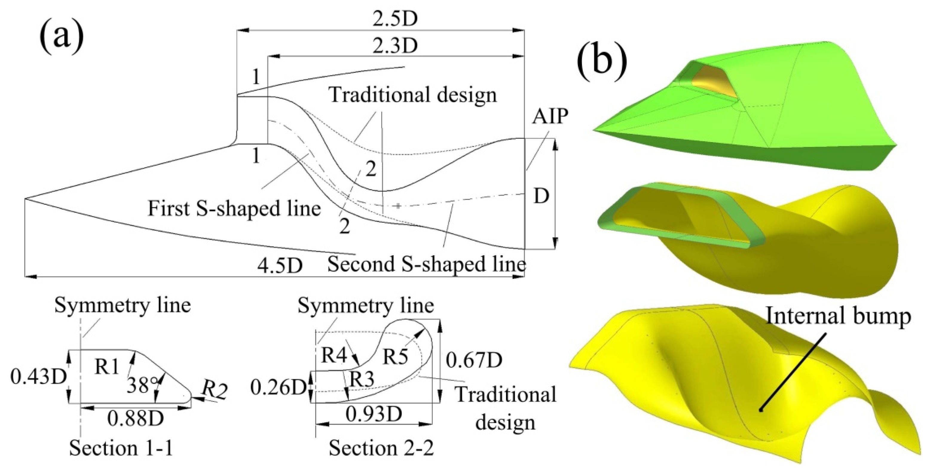
Figure 1.
(
a) Geometry and (
b) experimental setup of the serpentine inlet of NUAA Inlet Research Group [
33].
Figure 1.
(
a) Geometry and (
b) experimental setup of the serpentine inlet of NUAA Inlet Research Group [
33].
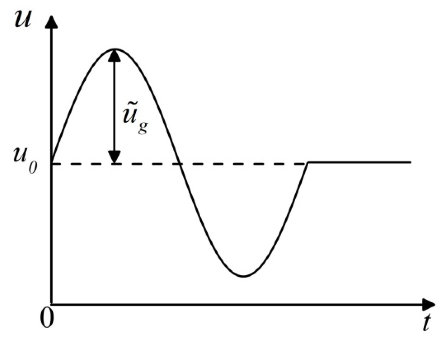
Figure 2.
Definition of the gust velocity profile of interest in this study.
Figure 2.
Definition of the gust velocity profile of interest in this study.
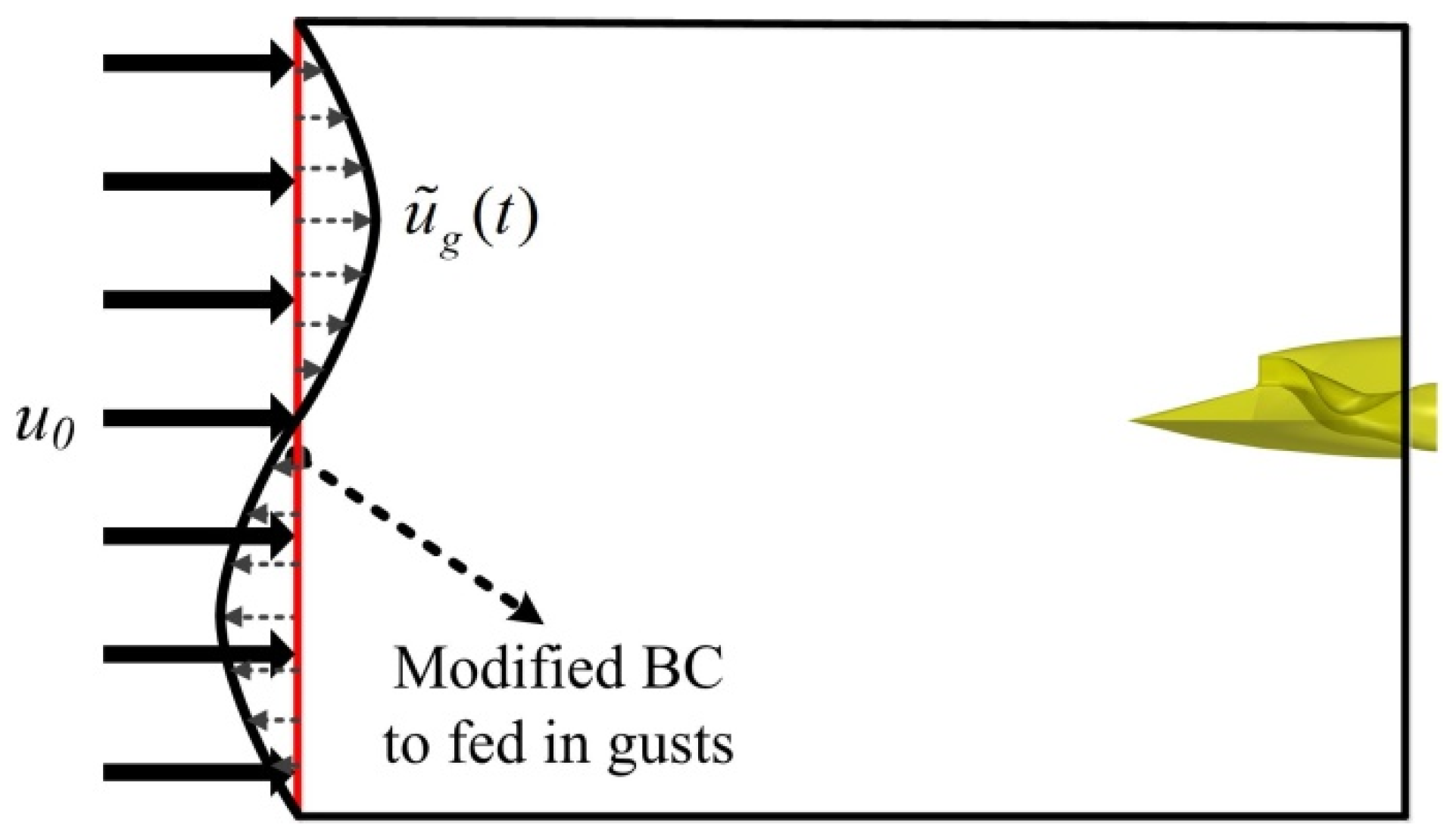
Figure 3.
Illustration of the implementation of the current FVM gust modeling method.
Figure 3.
Illustration of the implementation of the current FVM gust modeling method.
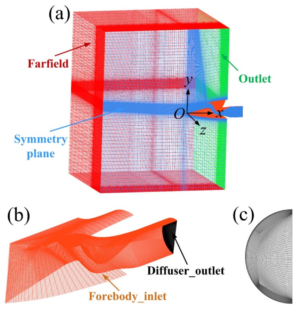
Figure 4.
Computational grid used in the current study: (a) Global view of the whole computational domain; (b) Close view of the surface mesh on the forebody-inlet integration; (c) Close view of the O-type mesh at the AIP.
Figure 4.
Computational grid used in the current study: (a) Global view of the whole computational domain; (b) Close view of the surface mesh on the forebody-inlet integration; (c) Close view of the O-type mesh at the AIP.
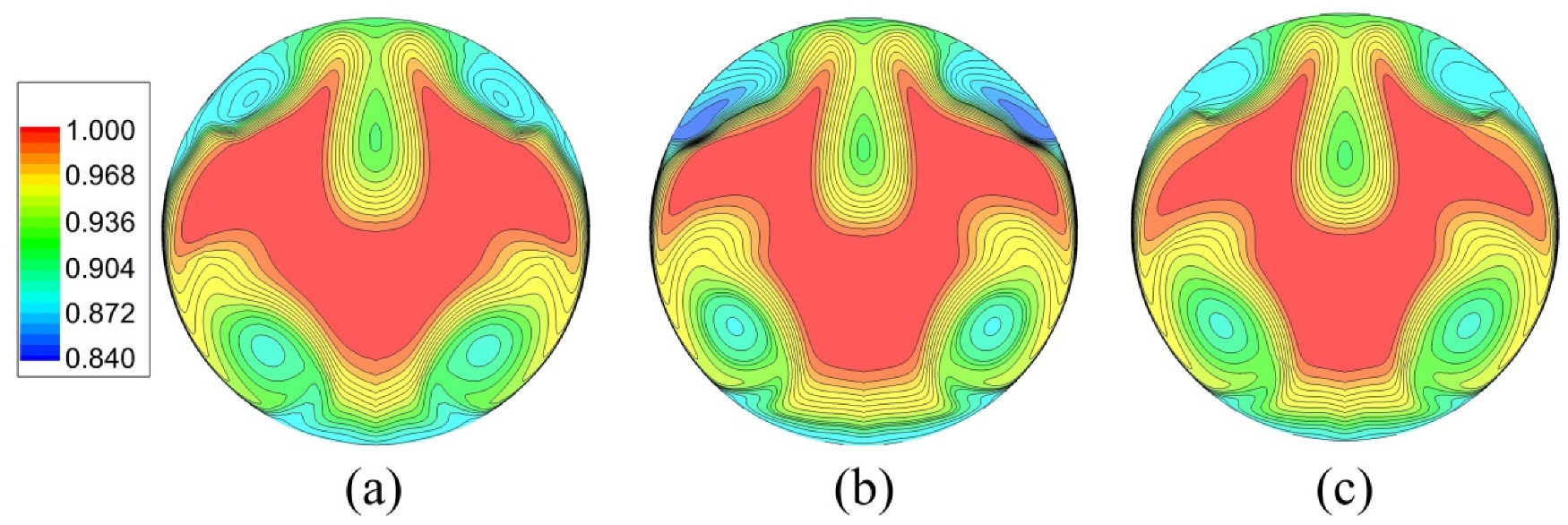
Figure 5.
Comparison of the total pressure contours at the AIP calculated with different levels of mesh resolutions at M = 0.7 and pAIP/p0 = 1.18: (a) Coarse grid; (b) Fine grid; (c) Dense grid.
Figure 5.
Comparison of the total pressure contours at the AIP calculated with different levels of mesh resolutions at M = 0.7 and pAIP/p0 = 1.18: (a) Coarse grid; (b) Fine grid; (c) Dense grid.
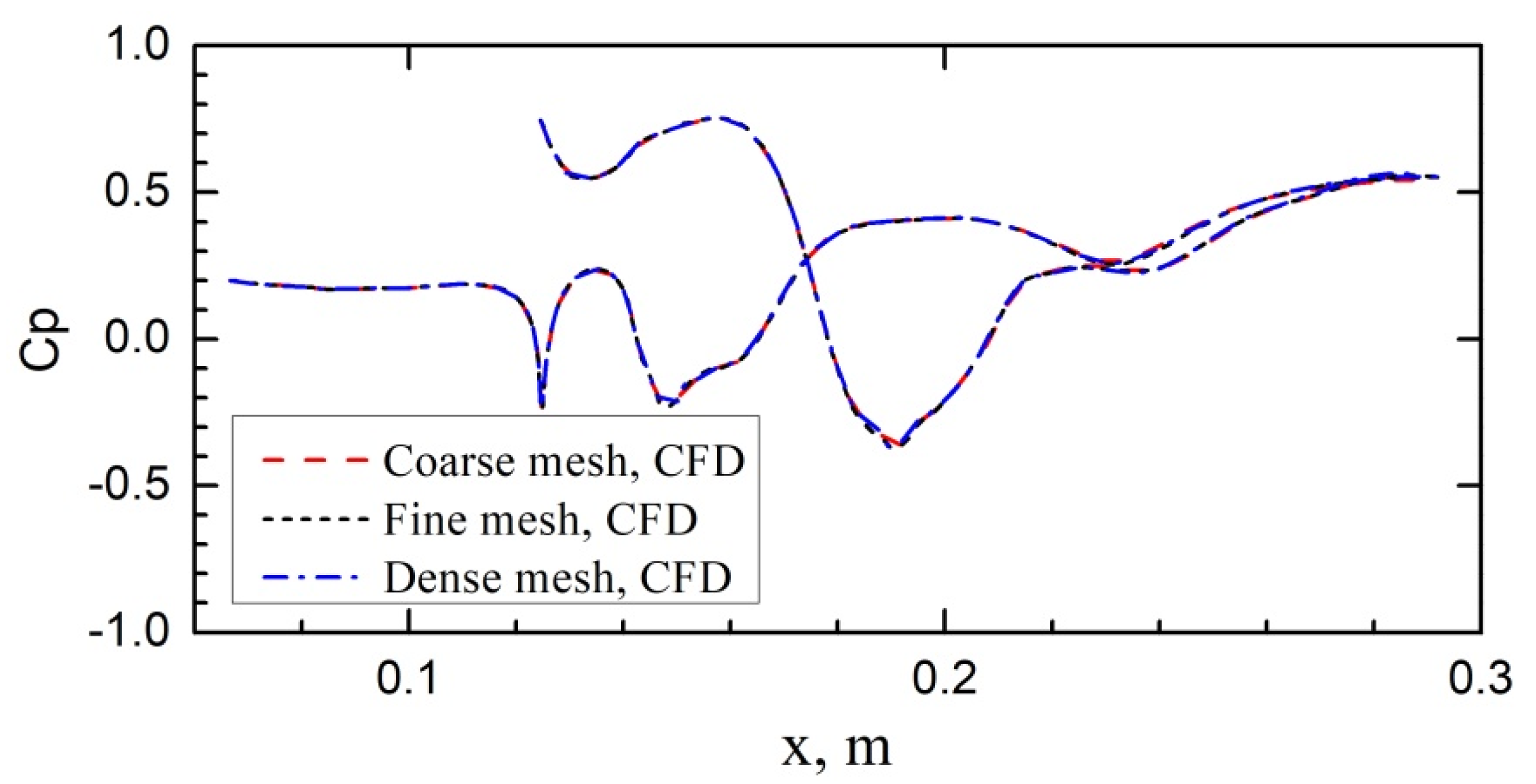
Figure 6.
Surface static pressure distributions calculated with different-sized meshes at M = 0.7 and pAIP/p0 = 1.18.
Figure 6.
Surface static pressure distributions calculated with different-sized meshes at M = 0.7 and pAIP/p0 = 1.18.
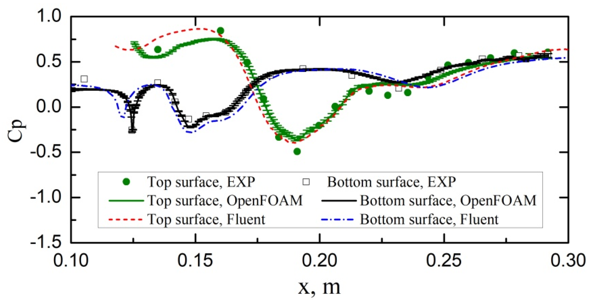
Figure 7.
Comparison of the surface static pressure results between the experiment and both CFD methods at M = 0.7 and pAIP/p0 = 1.18 in the absence of gust.
Figure 7.
Comparison of the surface static pressure results between the experiment and both CFD methods at M = 0.7 and pAIP/p0 = 1.18 in the absence of gust.
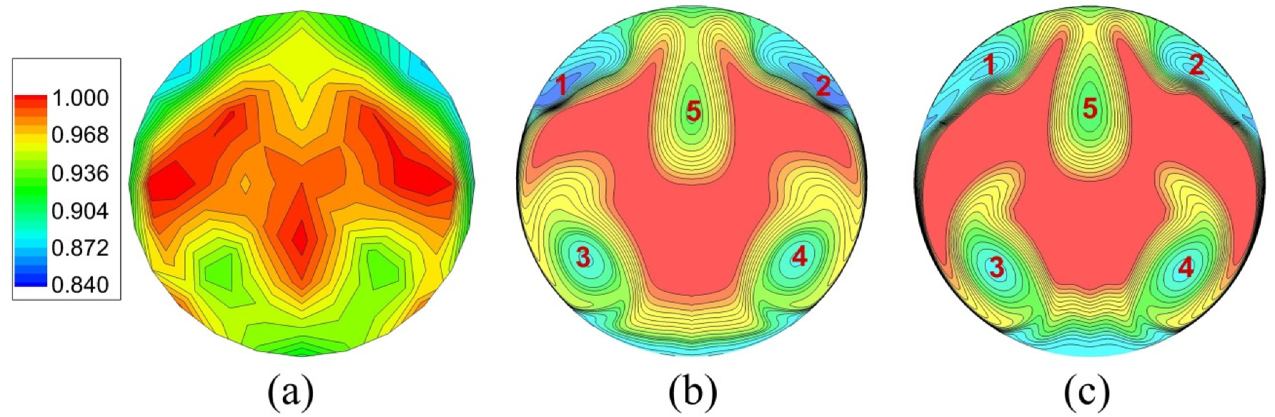
Figure 8.
Comparison of the total pressure contours at the AIP between (
a) the experiment, (
b) the current OpenFOAM solver, and (
c) the previous Fluent solver [
33] at M = 0.7 and
pAIP/
p0 = 1.18.
Figure 8.
Comparison of the total pressure contours at the AIP between (
a) the experiment, (
b) the current OpenFOAM solver, and (
c) the previous Fluent solver [
33] at M = 0.7 and
pAIP/
p0 = 1.18.
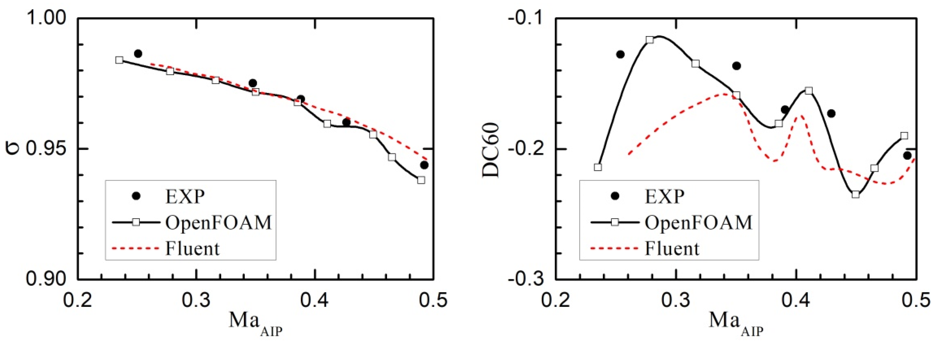
Figure 9.
Comparison of the inlet performance results between the experiment and both CFD methods at various AIP Mach numbers (M = 0.7).
Figure 9.
Comparison of the inlet performance results between the experiment and both CFD methods at various AIP Mach numbers (M = 0.7).
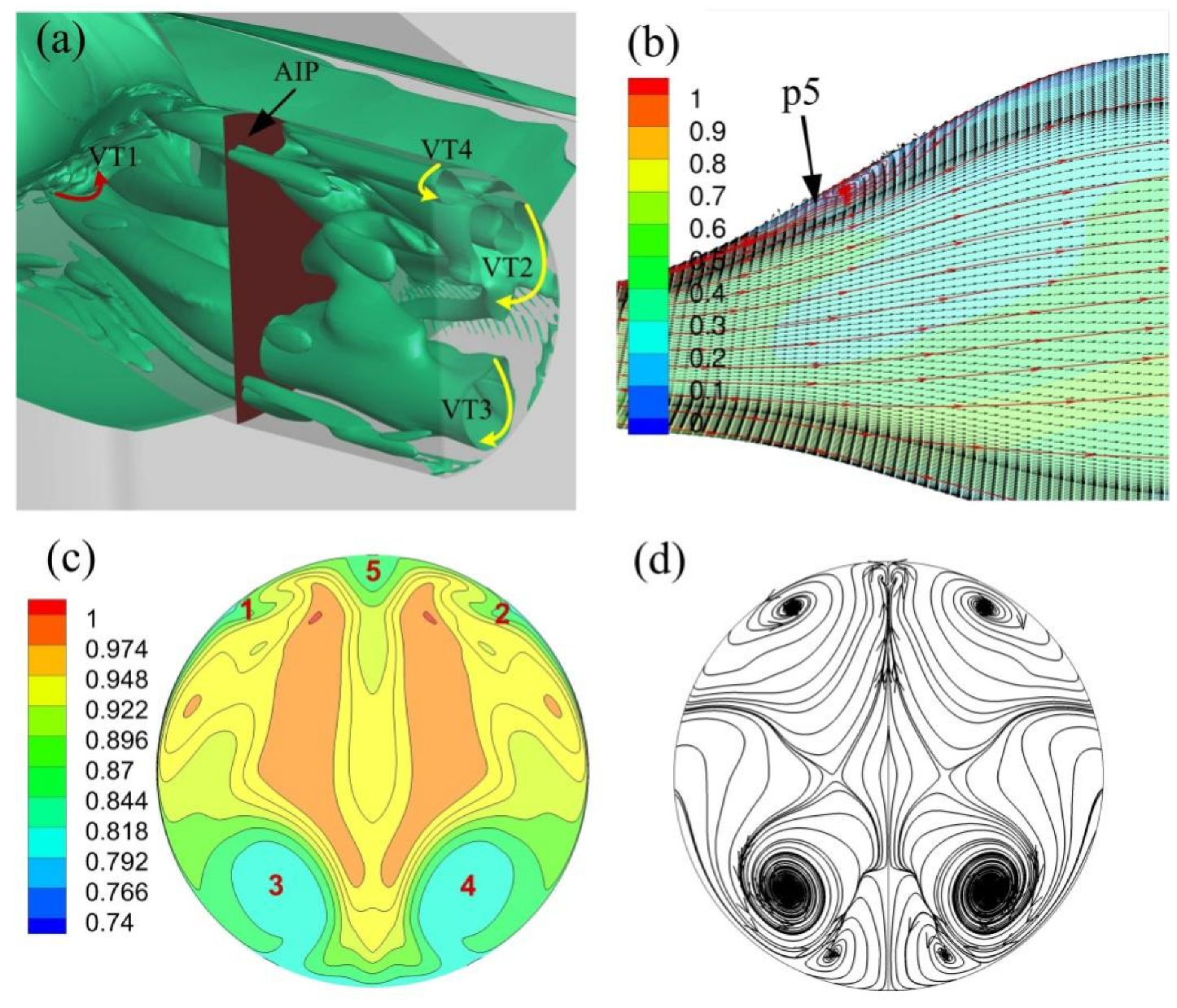
Figure 10.
Flow field characteristics of the serpentine inlet at M = 0.235 and pAIP/p0 = 0.85 under the no-gust condition: (a) the vortex tube (VT) structure, (b) Flow separation occurring at the lee side of the top surface coupled with the Mach number contour, (c) Total pressure contour at the AIP, and (d) Pattern of the secondary flow at the AIP.
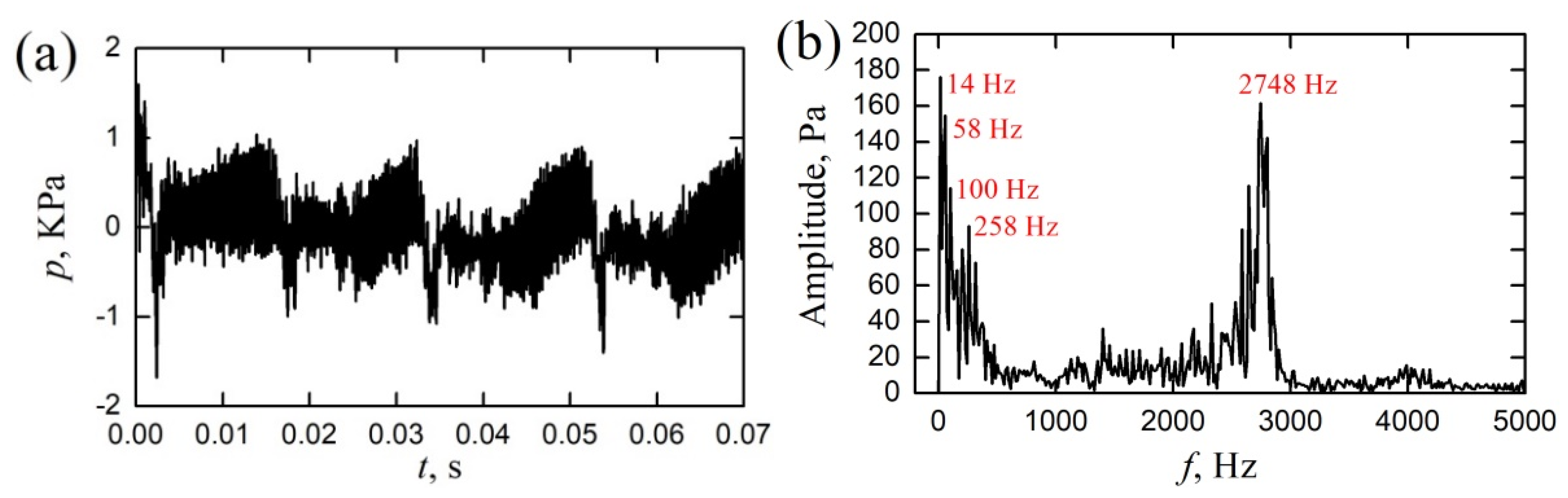
Figure 11.
(a) The unsteady fluctuation and (b) the spectrum of the wall static pressure probed at position p5.
Figure 11.
(a) The unsteady fluctuation and (b) the spectrum of the wall static pressure probed at position p5.
Figure 12.
(a) The unsteady fluctuation and (b) the spectrum of the total pressure recovery at the AIP.
Figure 12.
(a) The unsteady fluctuation and (b) the spectrum of the total pressure recovery at the AIP.
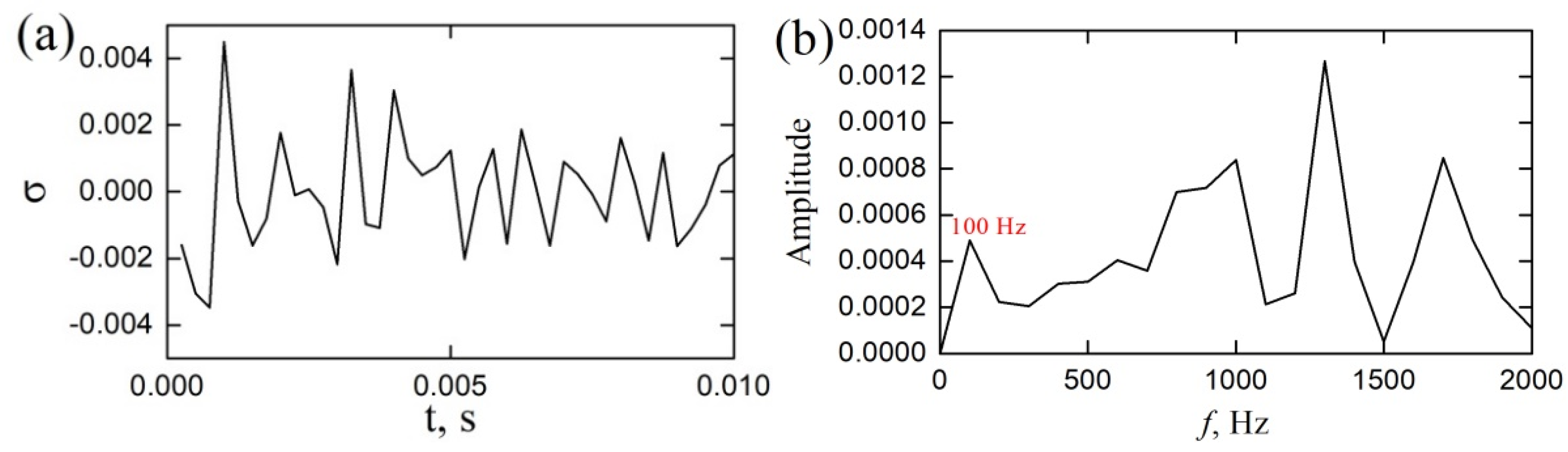
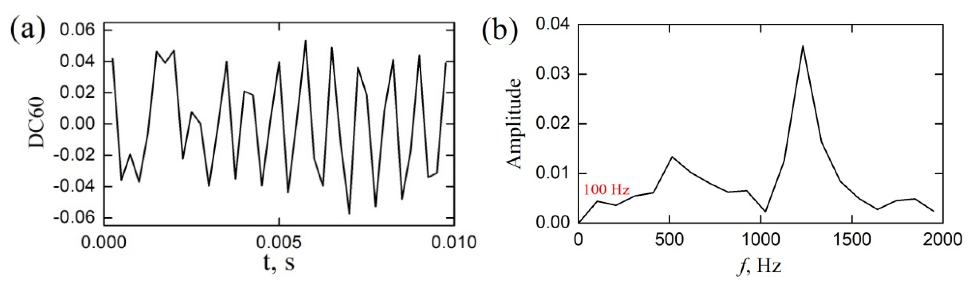
Figure 13.
(a) The unsteady fluctuation and (b) the spectrum of the total pressure distortion at the AIP.
Figure 13.
(a) The unsteady fluctuation and (b) the spectrum of the total pressure distortion at the AIP.
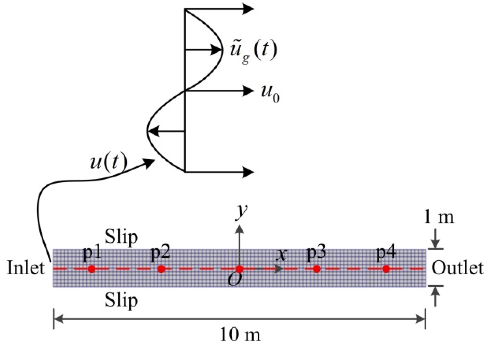
Figure 14.
Illustration of the gust model and the probed positions for characterization of the horizontal sinusoidal gusty inflow condition implemented by this study.
Figure 14.
Illustration of the gust model and the probed positions for characterization of the horizontal sinusoidal gusty inflow condition implemented by this study.
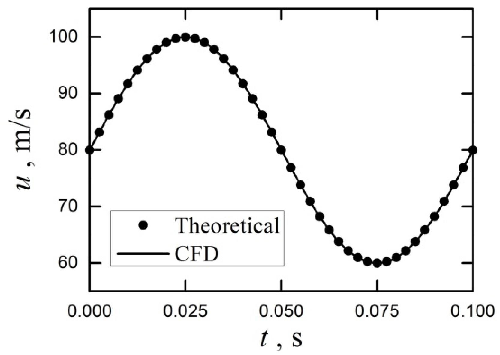
Figure 15.
Comparison of the horizontal gust velocity between the theoretical value and the current CFD result.
Figure 15.
Comparison of the horizontal gust velocity between the theoretical value and the current CFD result.
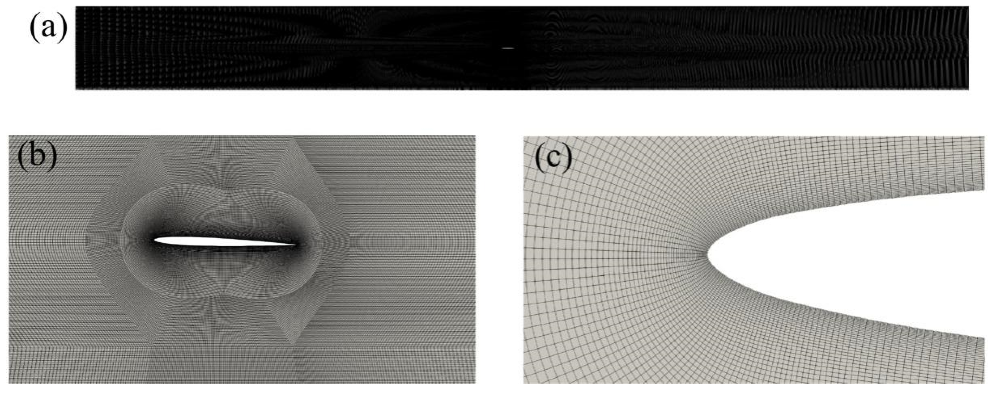
Figure 16.
Computational grid for simulation of the gust responses of the NACA 0006 airfoil: (a) Global view of the whole computational domain; (b) Close view of the mesh near the airfoil; (c) Close view of the O-type mesh at the leading edge of the airfoil.
Figure 16.
Computational grid for simulation of the gust responses of the NACA 0006 airfoil: (a) Global view of the whole computational domain; (b) Close view of the mesh near the airfoil; (c) Close view of the O-type mesh at the leading edge of the airfoil.
Figure 17.
Comparisons of (a) the 1-cosine and (b) sinusoidal vertical gust velocity profiles between the theoretical and current CFD results, followed by comparisons of lift coefficient (CL) responses of the NACA 0006 airfoil to the two gusts in (c) and (d), respectively.
Figure 17.
Comparisons of (a) the 1-cosine and (b) sinusoidal vertical gust velocity profiles between the theoretical and current CFD results, followed by comparisons of lift coefficient (CL) responses of the NACA 0006 airfoil to the two gusts in (c) and (d), respectively.
Figure 18.
Effects of the number of gust discretization intervals for a full-period gust, N, on the CFD results of the gust velocity at three probe locations in the symmetry plane (a) in the farfield, (b) at the middle of the entrance of the diffuser and (c) at the middle of the AIP position; Effects of N on (d) the total pressure recovery, (e) circumferential distortion and (f) outlet Mach number at the AIP. The simulated gust frequency is f = 50 Hz and amplitude m/s.
Figure 19.
Velocity vector, streamline, and Mach number distribution near the flow separation zone for the gust case of f = 100 Hz and m/s at the four instants.
Figure 19.
Velocity vector, streamline, and Mach number distribution near the flow separation zone for the gust case of f = 100 Hz and m/s at the four instants.
Figure 20.
Static pressure distributions on the top surface of the inlet under the no-gust condition and at different phases of the gust (f = 100 Hz and m/s) at M = 0.235 and pAIP/p0 = 0.85: (a) the overall view and (b) amplified view in the adverse-pressure-gradient zone.
Figure 20.
Static pressure distributions on the top surface of the inlet under the no-gust condition and at different phases of the gust (f = 100 Hz and m/s) at M = 0.235 and pAIP/p0 = 0.85: (a) the overall view and (b) amplified view in the adverse-pressure-gradient zone.
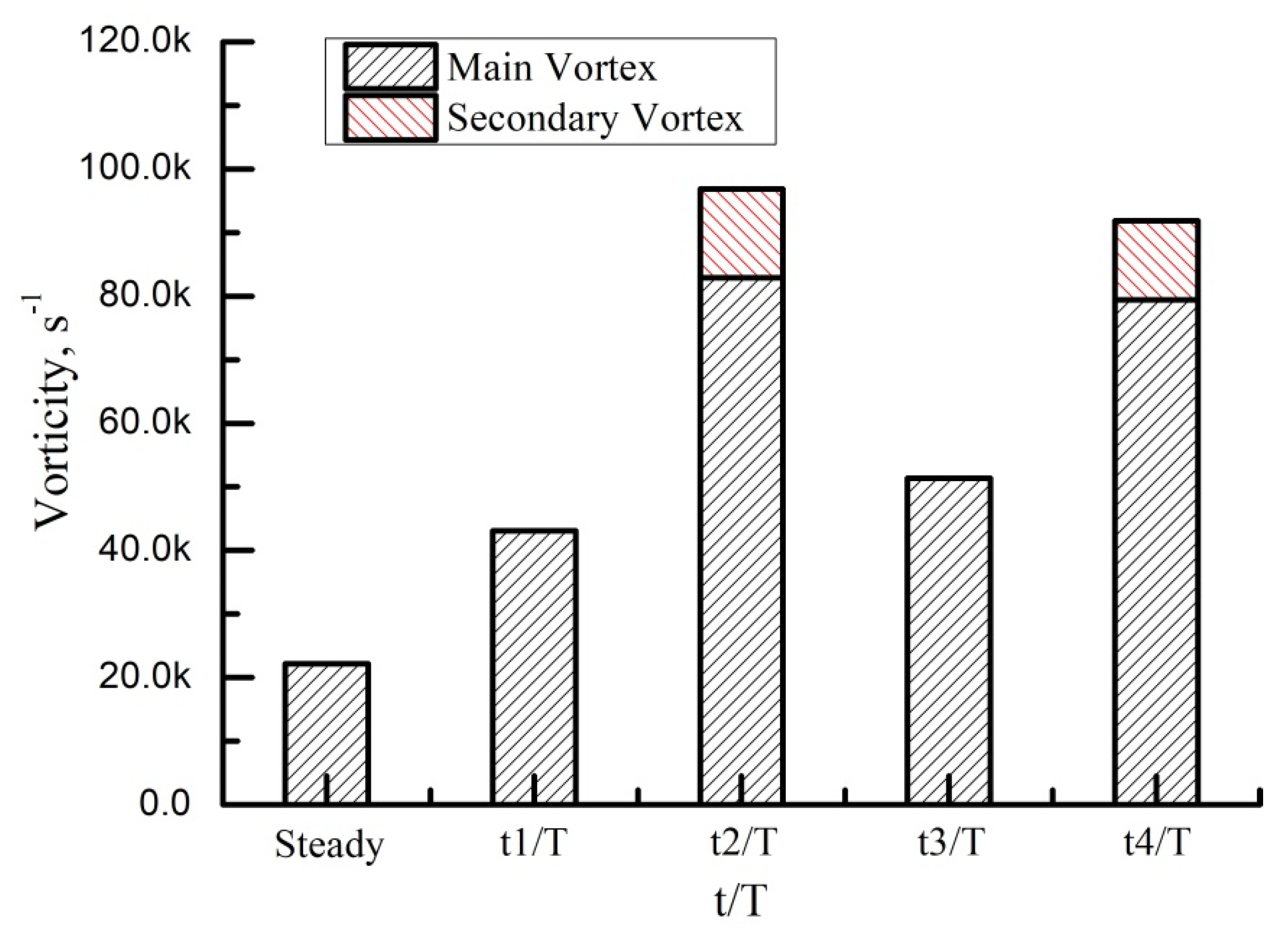
Figure 21.
Vorticity of the vortex cores shown in
Figure 19. For both the cases with two vortex cores, the upstream one has the larger vorticity and is thus named as ‘main vortex’.
Figure 21.
Vorticity of the vortex cores shown in
Figure 19. For both the cases with two vortex cores, the upstream one has the larger vorticity and is thus named as ‘main vortex’.
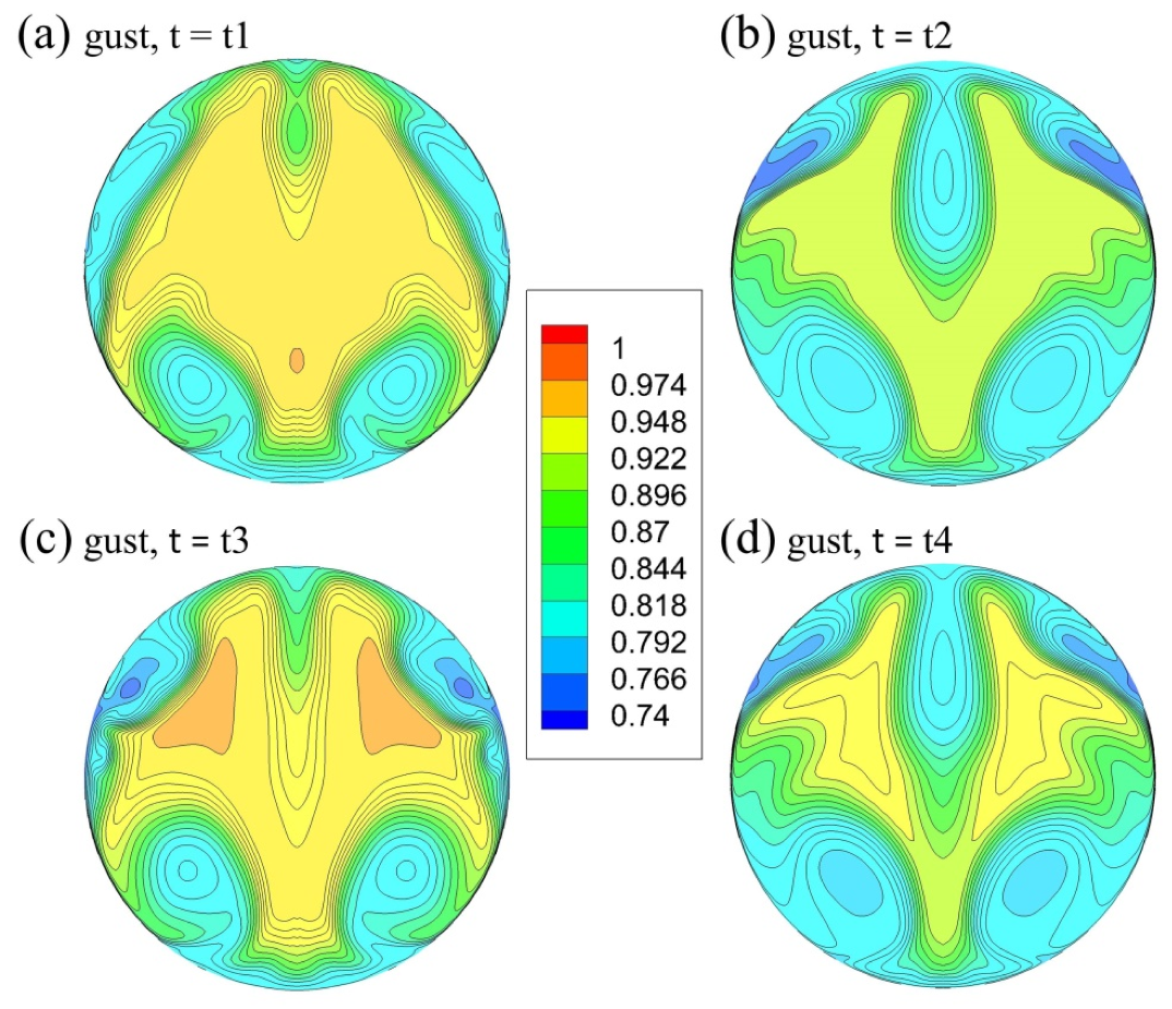
Figure 22.
Total pressure contours at the AIP at four instances of the gust case of f = 100 Hz and m/s.
Figure 22.
Total pressure contours at the AIP at four instances of the gust case of f = 100 Hz and m/s.
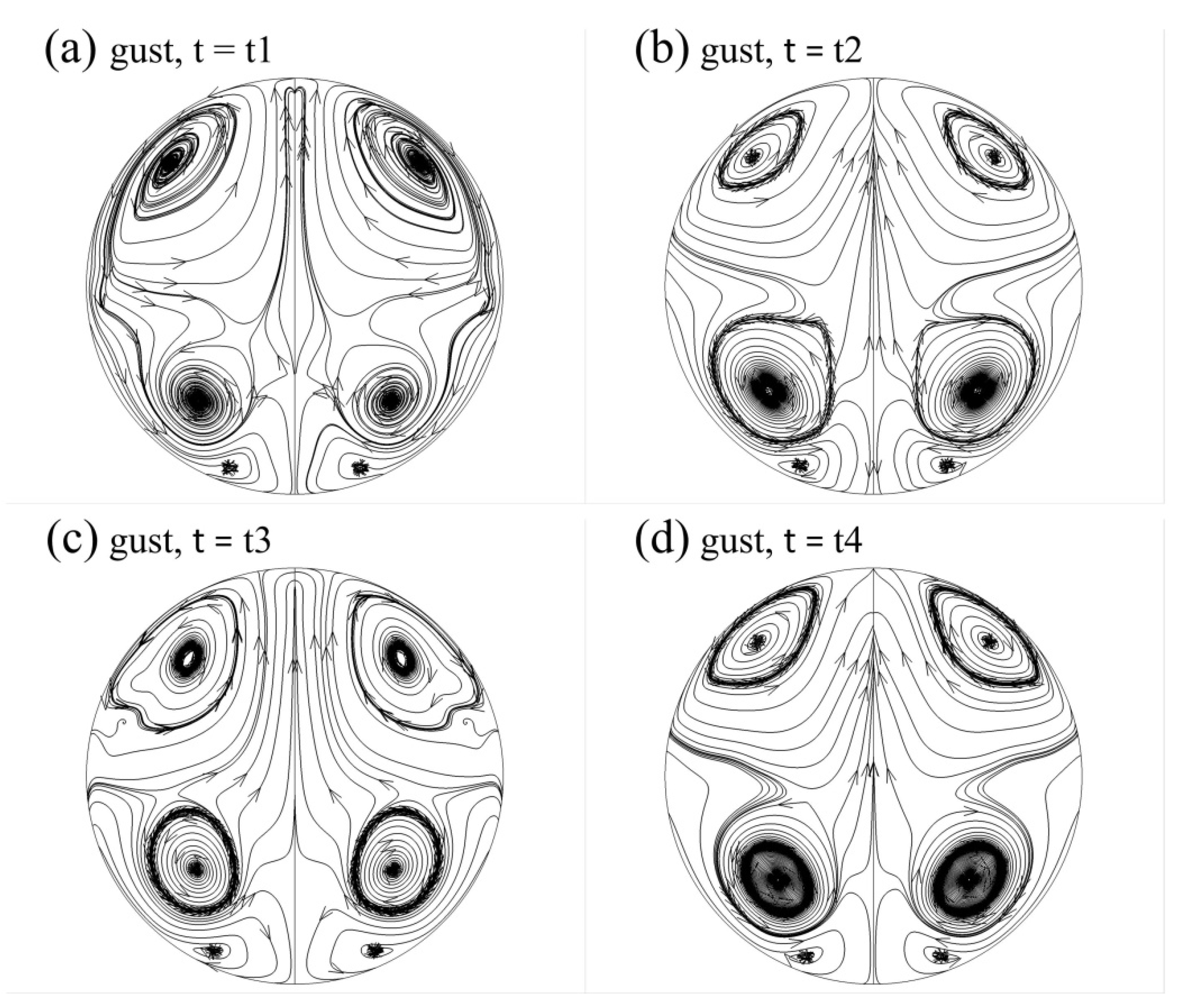
Figure 23.
Streamline distributed at the AIP at four instances of the gust case of f = 100 Hz and m/s.
Figure 23.
Streamline distributed at the AIP at four instances of the gust case of f = 100 Hz and m/s.
Figure 24.
Time histories of the inlet performance at various gust frequencies combined with the amplitude of m/s.
Figure 24.
Time histories of the inlet performance at various gust frequencies combined with the amplitude of m/s.
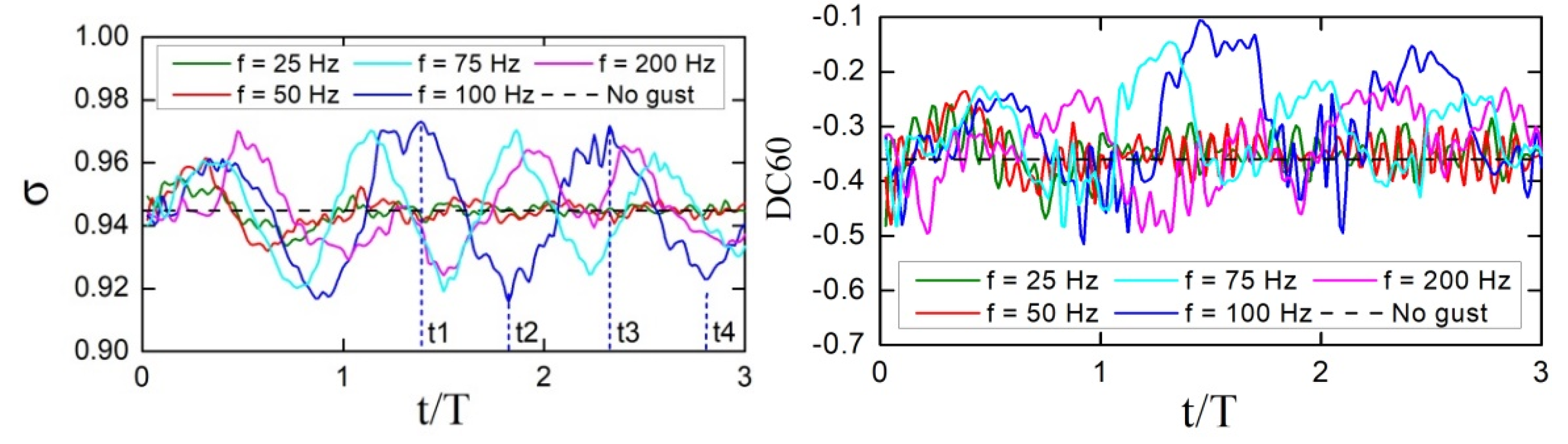
Figure 25.
Performance responses of the inlet to the gusts over a wide range of frequency at the constant amplitude of m/s. The mean results of the no-gust case are also shown for comparison.
Figure 25.
Performance responses of the inlet to the gusts over a wide range of frequency at the constant amplitude of m/s. The mean results of the no-gust case are also shown for comparison.
Figure 26.
Time histories of the inlet performance responses to the gusts with various amplitudes at a frequency of f = 50 Hz.
Figure 26.
Time histories of the inlet performance responses to the gusts with various amplitudes at a frequency of f = 50 Hz.
Figure 27.
The inlet performance responses to the gusts with various amplitudes at a frequency of f = 50 Hz. The results of the no-gust case are also presented for comparison purpose.
Figure 27.
The inlet performance responses to the gusts with various amplitudes at a frequency of f = 50 Hz. The results of the no-gust case are also presented for comparison purpose.
Figure 28.
Non-dimensional amplitudes of the total pressure recovery and distortion responses for the non-dimensional gust frequency fD/u0 and non-dimensional gust amplitude , respectively.
Figure 28.
Non-dimensional amplitudes of the total pressure recovery and distortion responses for the non-dimensional gust frequency fD/u0 and non-dimensional gust amplitude , respectively.
Table 1.
Main geometric parameters of the ultra-compact serpentine inlet.
Table 1.
Main geometric parameters of the ultra-compact serpentine inlet.
| Parameter | Value |
|---|
| Diameter of the AIP | D (65 mm) |
| Distance between the forebody tip and the inlet | 2.0 D |
| Total length of the inlet | 2.5 D |
| Length of the diffuser | 2.3 D |
| Vertical offset of the diffuser | 0.66 D |
Table 2.
Boundary condition settings for the computational domain.
Table 2.
Boundary condition settings for the computational domain.
| Boundary | | | p | T | |
|---|
| Farfield | inletOutlet | inletOutlet | freestreamPressure | inletOutlet | freestreamVelocity |
| Outlet | inletOutlet | inletOutlet | fixedValue | inletOutlet | zeroGradient |
| Symmetry plane | symmetry | symmetry | symmetry | symmetry | symmetry |
| Forebody_inlet | kqRWallFunction | omegaWallFunction | zeroGradient | zeroGradient | noSlip |
| Diffuser_outlet | inletOutlet | inletOutlet | fixedValue | inletOutlet | zeroGradient |
Table 3.
Inlet performance calculated with different resolved meshes at M = 0.7 and pAIP/p0 = 1.18.
Table 3.
Inlet performance calculated with different resolved meshes at M = 0.7 and pAIP/p0 = 1.18.
| Data Source | Number of Grid Cells | σAIP | Error of σAIP |
|---|
| EXP. [33] | — | 0.961 | — |
| Coarse mesh | 2.48 million | 0.968566 | 1.039 × 10⁻³ |
| Fine mesh | 4.20 million | 0.967687 | 1.597 × 10⁻⁴ |
| Dense mesh | 5.95 million | 0.967527 | — |
Table 4.
Values of the material parameters for the inlet gust response calculations.
Table 4.
Values of the material parameters for the inlet gust response calculations.
| Variable | Value |
|---|
| Ambient pressure, p0, Pa | 101,325 |
| Inlet exit pressure, pe, Pa | 86,126.25 |
| Air density, ρ0, kg/m3 | 1.17 |
| Air dynamic viscosity, μ0, Pa·s | 1.82 × 10⁻⁵ |
| Ambient temperature, T0, K | 300 |
| Inlet exit temperature, Te, K | 300 |
| Freestream Mach number, M | 0.235 |
| Freestream velocity, u0, m/s | 80 |
| Gust frequency, f, Hz | 25, 50, 75, 100, 125, 150, 175, 200, 225, 250, 275, 300 |
| Gust amplitude, , m/s | 4, 8, 12, 16, 20 |
Table 5.
Comparison of the maximum amplitudes of total pressure recovery and distortion fluctuations between the cases without/with gusts.
Table 5.
Comparison of the maximum amplitudes of total pressure recovery and distortion fluctuations between the cases without/with gusts.
| Variable | Without Gust | With Gust |
|---|
| σm/σ0 | 0.48% | 3.83% |
| DC60m/DC600 | 16.00% | 56.39% |


