An Approach to the Preliminary Sizing and Performance Assessment of Spaceplanes’ Landing Parafoils

Abstract

In this new era of space exploration, reusability and lower environmental impact are critical drivers in pursuing innovative solutions for access to space. One of these leading solutions is the Space Rider, a European reusable space plane with the ability to be both an “access to space” and a “return from space”. Following the lesson learned from the Intermediate eXperimental Vehicle (IXV) design and testing, the Space Rider will be equipped with a parafoil to enhance manoeuvrability during landing. Politecnico di Torino (PoliTO), in collaboration with Thales Alenia Space Italy (TAS-I), has developed an integrated tool to assess the landing performances of spaceplanes equipped with parafoils during conceptual design. The presented approach fuses sizing, dynamic models, guidance and control algorithms to provide a software suite for the rapid prototyping, sizing and performance assessment of spaceplanes’ parafoils. This paper details the implementation, mathematical background, validation and lessons learned behind the different software modules.

1. Introduction

Parafoils, or ram–air parachutes, are decelerators with high efficiency and good manoeuvrability. They have multiple civil and military applications for cargo delivery on Earth [1,2,3]. The typical application of these decelerators deals with a non-collaborative payload, modelled only by its weight, volume and drag coefficient.

However, lately, the use of parafoil to enhance the landing capabilities of lifting bodies has become an interesting field of study. Starting from the X-38 experience [3], a parafoil will be used to enable the landing of the European reusable spaceplane Space Rider [4]. In more detail, the parafoil will help the system to safely land on a spaceport runaway after the harsh re-entry phase [5] instead of employing the IXV splash-down solution as a landing scenario [6].

Therefore, during the initial conceptualization phase of these parafoil-enabled landing solutions, different configurations of parafoil sizes and payload weights need investigation. The objective is to rapidly assess the performances of the diverse configurations to trade them before a detailed design.

However, the existing in-depth studies are usually unsuitable for rapid prototyping and a rapid investigation of system performances.

On the study of parafoil design, different analyses have been conducted on dynamic models for parafoil [1,7,8,9,10]. Other studies focused on the in-depth aerodynamic formulations [11,12,13] or on the optimal terminal guidance of ram–air parachutes, as in [14,15]. Those precise and in-depth analyses are performed on models that require a set of data that is usually not available at a high level of design.

To answer this lack of a rapid prototyping tool where the spaceplane-parafoil system landing performance can be assessed at a high-design level, Politecnico di Torino, with the advice of Thales Alenia Space Italy (TAS-I), developed a tool called PIMENTO (ParafoIl ModElliNg ToOl). The tool is built from mathematical and similarity models typical of aerospace design and already employed in aircraft application, as in [16,17]. 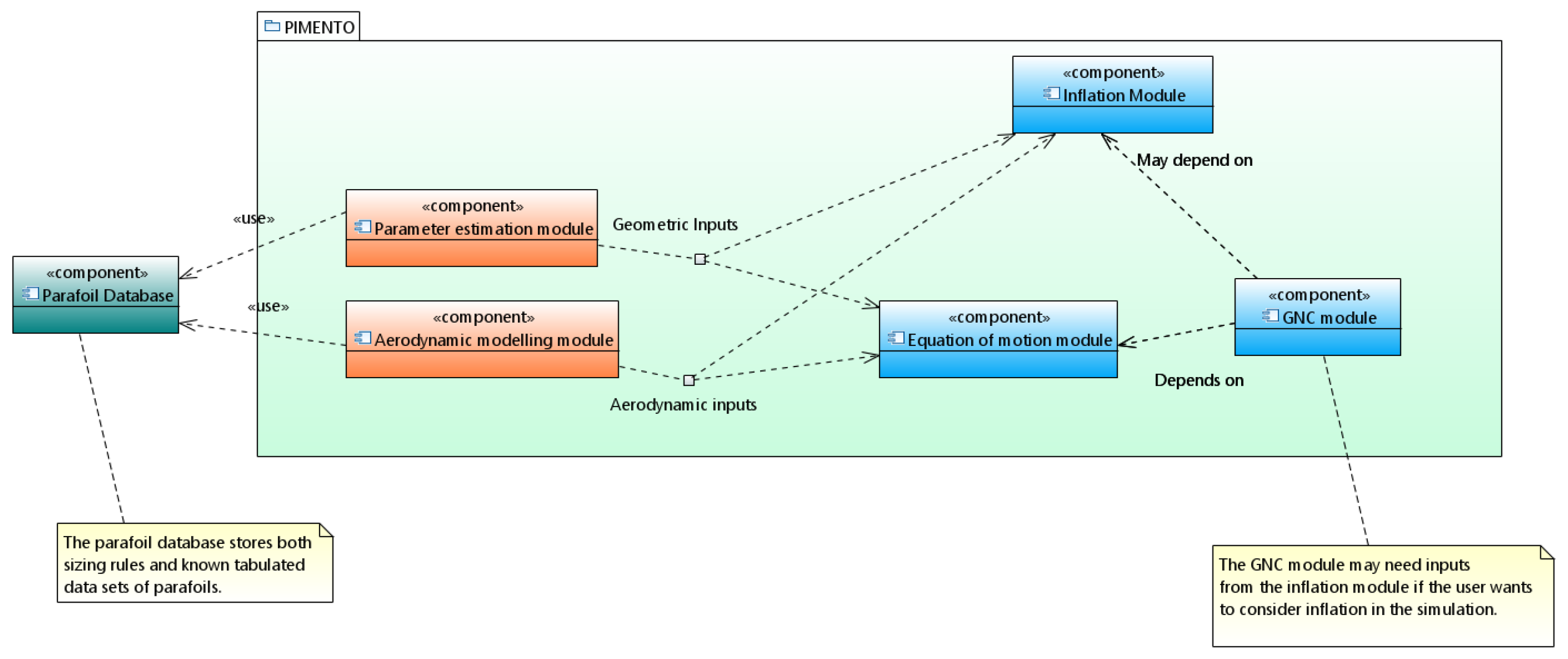Figure 1 shows the logical flow of PIMENTO, while Figure 2 details the modules of the software and their interactions. The tool includes a parafoil sizing module, a parafoil aerodynamic estimation module, an inflation module, and a model for guidance, navigation, and control. More precisely, the aim of PIMENTO is to provide a simulation environment that can: (i) estimate preliminary parafoil sizing parameters, (ii) generate a feasible reference trajectory to land near the target safely using a three degrees of freedom model (DOF), (iii) simulate the performances and overall behaviour of the parafoil–payload system during a controlled descent employing a six DOF or a nine DOF, and (iv) estimate initial position and velocity of the parafoil at full deployment thanks to a preliminary inflation model estimation.

The paper proposes a design approach that starts from the definition of the parafoil shape and then tests its feasibility, allowing the rapid analysis of different flight configurations and their impact on the performance of the overall system design. Its output is a preliminary design defined as in the NASA System Engineering Handbook [18], where the product of the preliminary design phases is a feasible system concept that can attain the expected performances defined by the stakeholders [19].

The paper details the overall rapid prototyping approach, focusing on the different software modules to guide the reader throughout the proposed design process. The mathematical background of each module has been validated using reference data provided by TAS-I drop tests or available from literature.

The study’s novelty lies in creating an integrated framework that fuses sizing, dynamic models, guidance and control algorithms for the rapid design of parafoils. Most analyses of novel parafoils rely on steady-state simulations. The parafoil size and aerodynamics are usually mutated from existing parafoil used for precision delivery systems [1]. If nothing similar exists, scaling by similarity models is used [1]. The work presented in this paper goes further, analysing how the defined design would perform in a realistic landing scenario with different spirals and turns, not only looking at a steady state simulation. In the literature, the landing and manoeuvring capabilities are considered during the in-depth GNC (Guidance, Navigation and Control) study that follows the preliminary sizing of parafoils. This approach works well with non-collaborative cargo payloads. If the payload is a lifting body, its position and aerodynamics may influence the delivery system’s overall capabilities. Hence, an assessment routine like the one suggested in this paper can help avoid expensive redesigns when problems arise during testing.

Diving more in detail into the state of the art of parafoil-related research, the study of the dynamics of parafoil for Earth applications has been extensively analyzed in [1,7,8,9,10,20,21]. These analyses start with a robust set of geometrical and aerodynamic data.

One particularly remarkable dynamic model is defined in [22]. Thanks to its precise identification of the overall centre of mass of the parafoil–payload system based on initial geometry, the [22] model is reasonably practical during preliminary design phases. The [22] model has been developed for Small autonomous Parafoil Landing Experiment (ALEX) parafoil, and it has been validated with its test results [23]. In [22], the focus rapidly shifts toward a detailed analysis of the GNC algorithm after the definition of the dynamic model. In the studies of [1,7,8], the parafoil dynamic is highly linked to the study of different GNC architectures suitable for the mission at hand. The employed models start from six DOF and evolve into multi-body models. During preliminary design studies, three or four degrees of freedom models are preferred for their simplicity: they do not require an in-depth study of the GNC [1]. This is another innovation of PIMENTO that incorporates a simple GNC module to provide a complete parafoil preliminary sizing and performance assessment.

The study in [12] proposes a simulator that joins a six degrees of freedom model with an in-house aerodynamic estimation tool based on the panel method. However, the in-depth aerodynamic study requires a good knowledge of the principal characteristics of the parafoil, from geometry to the airfoil model. Nevertheless, it is a powerful tool that can be employed in the second design round when the initial trade-space analysis has determined the main feasible configurations.

Finally, many studies focused on designing and optimizing the terminal guidance of a delivery ram–air parachute, as in [14,24,25,26,27]. The typical reference trajectory is based on two spirals and a final turn leg that aligns the parafoil with the landing runaway. A similar simplified reference trajectory is used in PIMENTO to evaluate the latero-directional stability and manoeuvrability of the identified design.

All these analyses are complementary to the presented tool and methodology, where the target is an initial assessment of the parafoil-spaceplane system performances.

The following chapters are organized as follows: Section 2 would focus on (i) the definition of the parameter estimation, (ii) the aerodynamic modelling, (iii) the equations of motion, (iv) the navigation, the guidance model and the control model, and (v) the inflation model, Section 3 presents the main results of the tool, and Section 4 provides an overview of the performed work and the future planned work.

2. Methods and Materials

2.1. Parafoil–Payload System Parameters Estimation

During the preliminary design of a parafoil–payload system, the designers may have a rough idea of the payload weight and the possible dimensions of the parafoil [1]. Therefore, the first and natural step of the proposed approach is to estimate the ram–air parachutes’ geometrical characteristics given a weight estimation of the payload and a possible surface area.

The mathematical formulation detailed in [1,11] has been used in PIMENTO to estimate the missing parafoil parameters. The formulas are summarized in

Table 1. Parafoil geometrical parameters’ estimation [1,11].

Parameter	Formulation
Canopy area	S = b * c
Aspect ratio	AR = b/c
Canopy span	$b=\sqrt{(S\ast AR)}$
Canopy chord	$c=\sqrt{(S/AR)}$
Canopy lines	R = 0.6 * b to R = 0.8 * b
Canopy thickness	t = (0.1–0.15) * c
Parafoil canopy height	a = b * t/c
Anhedral angle	$ϵ$ = b/2R
Harness Length	$l_{ha}$ = (0.15–0.45) * R
Number of suspension lines	ceil (S/1.11)
Diameter lines	2.5 mm

. A small database with the geometrical characteristics of known parafoils from [1,7,8,9,10,20,21,22] has been developed to estimate the aspect ratio, canopy lines length, and harness length. The database is used to fill the gaps of unknown geometrical parameters, and it can be used to estimate a first parafoil surface when it is unknown.

2.2. Aerodynamic Modelling

The aerodynamic modelling of parafoil during the preliminary design is crucial in assessing its performance. Therefore, different preliminary modelling strategies have been proposed for the parafoil aerodynamic coefficient estimation in [11,28,29,30].

All the proposed studies provide a good approximation of the longitudinal aerodynamics of parafoils. However, the aerodynamic coefficients in the latero-directional plane are the ones that give most of the numerical instabilities during simulations. Ill-defined latero-directional aerodynamic coefficients would jeopardize the overall performance assessment. As previously mentioned, the preliminary assessments of parafoil capabilities focus on steady-state simulations. However, a parafoil needs to manoeuvre its descent with spirals during landing. Moreover, the application with lifting bodies calls for a holistic approach that evaluates the latero-directional manoeuvrability as well.

Therefore, to fulfil the objective of PIMENTO, a good assessment of the latero-directional coefficient is fundamental. Unfortunately, data from CFD simulations or experimental methods are not available during conceptual design, where very little is known about the parafoil.

Different solutions have been investigated following the studies in [11,28,31]. However, when the results were compared with the data provided by TAS-I, there was a more than acceptable agreement on the longitudinal plane but a poor one on the latero-directional.

An approach based on aerodynamic similarity is suggested to overcome this issue of aerodynamics characterization during the preliminary design phases. In the aerodynamic characterization work carried out in [1], the parameters that mostly affect parafoil aerodynamics are the (i) aspect ratio, (ii) the aerodynamic profile, and (iii) the parafoil curvature. The aspect ratio has the most impact. Therefore, as a first approximation, it is possible to correlate the wing aerodynamic coefficients with existing or tested parafoil wings, knowing the aspect ratio of the parafoil and considering its shape as fixed.

The final aerodynamic set used in PIMENTO is based on the same database created for the sizing rules. During the simulation, PIMENTO takes as input the aspect ratio of the analyzed parafoil and outputs a preliminary aerodynamic set based on a similar system. The analysis can be refined if the aerodynamic profile or the parafoil curvature are known. For example, the aerodynamic set used for the simulations in this paper is based on the X-38 parafoil because of a similar surface and aspect ratio to the system studied. The airfoil of the X-38 is slightly different from the one studied by TAS-I, but they belong to the same airfoil family.

However, the parafoil envisioned for the Space Rider has an L/D around 4 [15] while the X-38 had an $L/D\simeq 3.8$. This discrepancy is related to the slightly different shape of the airfoil. To better match the data provided by TAS-I, the longitudinal plane curves of $C_L$ and $C_D$ were adjusted keeping into account the airfoil and following the modelling rules for the longitudinal aerodynamic in [28]. The output curves had the same trend of the X-38 as expected because of the same aspect ratio and airfoil family. However, the $C_L$ curve is slightly shifted upward while the $C_D$ curve is shifted slightly downward. Hence, the latero-directional aerodynamic coefficients are derived from the X-38, while the longitudinal coefficients are slightly adjusted considering the airfoil.

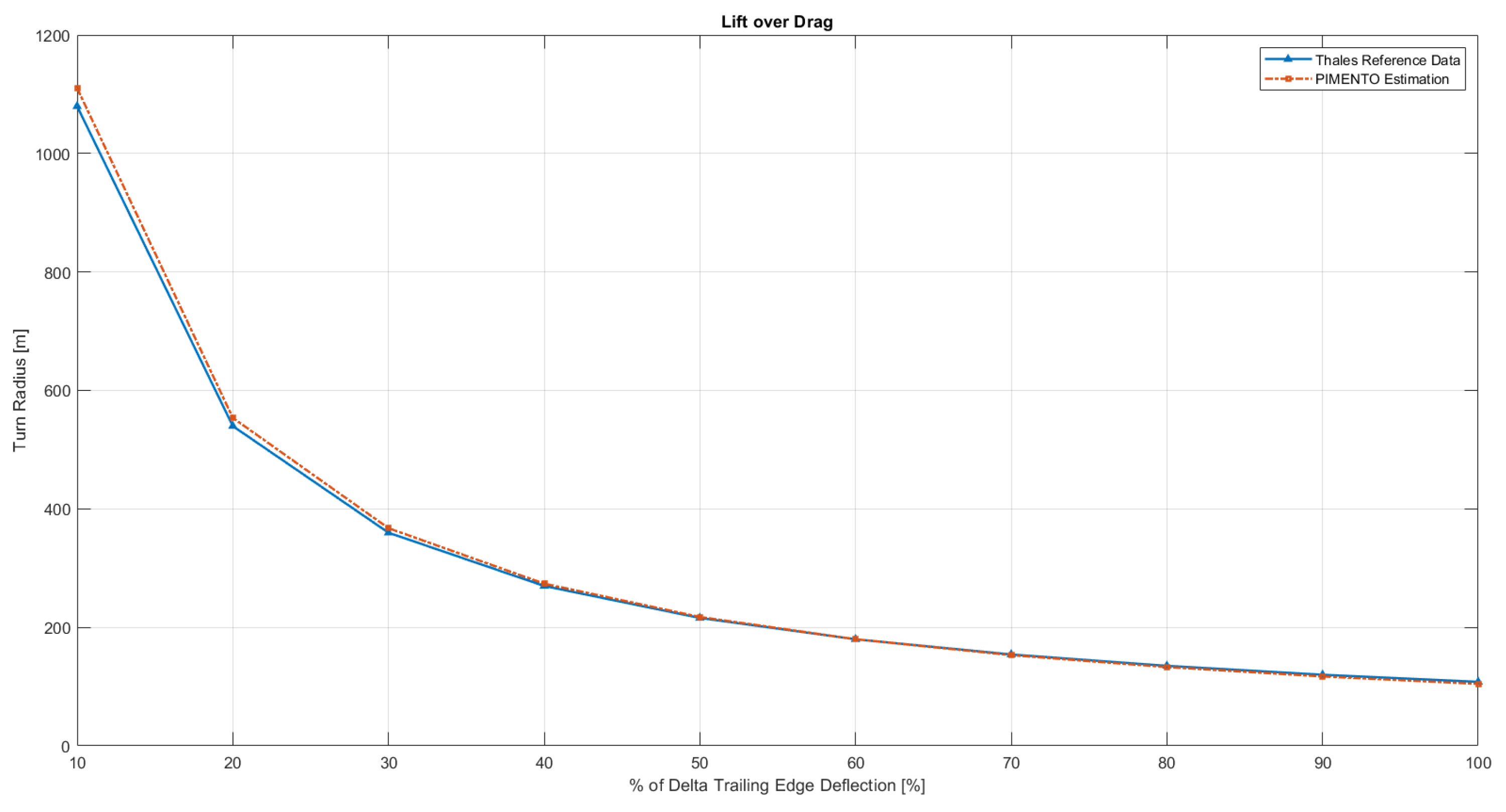
This aerodynamic dataset has been cross-validated with reference data provided by TAS-I on similar parafoil–payload configurations, Figure 3 and Figure 4. In Figure 3, the abscissa axis shows the percentage of symmetric deflection ${\delta }_s$ over a maximum deflection ${\delta }_{s_{max}}$ of 30 degrees of the trailing edge (Equation (1)).

While the abscissa of Figure 4 shows the difference ${\delta }_a$ between the right (${\delta }_{right}$) and left (${\delta }_{left}$) deflections of the trailing edge normalized with respect to the maximum difference ${\delta }_{a_{max}}$ (Equation (2)), the maximum difference ${\delta }_{a_{max}}$ in absolute value is obtained when deflecting only one side of the parafoil at 30 degrees:

$$\%{\delta }_s=\frac{{\delta }_s}{{\delta }_{s_{max}}}$$

(1)

$$\%{\delta }_a=\frac{|{\delta }_{right}-{\delta }_{left}|}{{\delta }_{a_{max}}}$$

(2)

Overall, the obtained results agree with the validation data provided, with a maximum error of less than 10%. Therefore, the error is in an acceptable range for fast prototyping studies during conceptual design [32].

2.3. Equation of Motion

After identifying the geometrical characteristics of the parafoil and its aerodynamics, the focus shifts toward the modelling of the parafoil–payload dynamics.

For the application of the Space Rider, one connection point is envisioned between the parafoil and the spaceplane, as shown in Figure 5. To model this interaction, PIMENTO runs six and nine DOF models. In the six DOF, the parafoil and the payload are analysed as a single system. Therefore, it is a model suitable for any connection between parafoil and payload. The nine DOF model separately analyses the two dynamics, parafoil and spaceplane, and then joins them at the connection point to study their dynamic interactions. Both models assume that the aerodynamics and shape of the parafoil are fixed after inflation.

This article focuses on the definition of the six DOF model because it is the most robust during preliminary design assessments while providing reliable initial results on the system performances.

On the other hand, the nine DOF model requires a better knowledge of the parafoil–payload parameters because it is more susceptible to numeric instabilities. It can be used during the following simulations when the relative position of the payload with respect to the parafoil is well-defined. Both models are adapted for the PIMENTO application from literature [1,20,22], and were extensively discussed and validated for their steady-state performances in [31,33]. For what concern the six DOF, both [1,22] models consider the effects of the apparent masses and rigging angle. However, the effects of the apparent masses are more precisely modelled in [1]. On the other hand, the model in [1] does not explicitly consider the effect of the added masses trapped in the inflated parafoil. Both models have been developed for the precise delivery of cargo. Therefore, the payload is identified only in terms of drag coefficient, reference area and weight. For the application of this paper, the effects of rigging angle, apparent masses, added masses and aerodynamics of the payload are considered in the model. Hence, this section details the complete mathematical formulation of the six DOF model and the second validation round performed with reference data provided by TAS-I. More precisely, this second performance assessment focuses on validating the model during manoeuvres in a windy environment. Therefore, it is complementary to the first verification in steady-state presented in [31,33].

For the nine DOF, the model in [20] is modified by adding the effects of the rigging angle and added masses. However, it would not be further detailed in this publication.

The equations are written for the barycentre B of the entire system and then permuted in the north-east-down (NED) reference system, Figure 5:

• The x-axis lays in a plane parallel to the one tangent to the planet surface at zero altitude and aims at the true North.
• The z-axis points down with the same direction of the system (parafoil and payload) gravity acceleration vector.
• The y-axis completes the right-handed Cartesian reference system, pointing eastward.

The figures in the results and validation sections refer to the NED reference system for the axis name except for the z-axis, called altitude in all the graphs showing the xz-plane.

Figure 5 shows the overall centre of mass B, the centre of mass of the parafoil P, the centre of mass of the spaceplane S, and the related forces and moments. The mathematical formulation is shown from Equations (3) to (7). The tensors and vectors in the equations are highlighted in boldface.

$$\left[\begin{array}{c}\mathbf{F}\\ \mathbf{M}\end{array}\right]=\left[\begin{array}{cc}m\ast {\mathbf{I}}_{3x3}+{\mathbf{M}}_f^{\prime }& -{\mathbf{M}}_f^{\prime }\ast \mathbf{S}\left({\mathbf{r}}_{BM}\right)\\ \mathbf{S}\left({\mathbf{r}}_{BM}\right)\ast {\mathbf{M}}_f^{\prime }& \mathbf{I}+{\mathbf{I}}_f^{\prime }-\mathbf{S}\left({\mathbf{r}}_{BM}\right)\ast {\mathbf{M}}_f^{\prime }\ast \mathbf{S}\left({\mathbf{r}}_{BM}\right)\end{array}\right]\left[\begin{array}{c}\dot{u}\\ \dot{v}\\ \dot{w}\\ \dot{p}\\ \dot{q}\\ \dot{r}\end{array}\right]$$

(3)

$$\mathbf{F}={\mathbf{F}}_a^p+{\mathbf{F}}_a^s+{\mathbf{F}}_g-\left(m\right)\ast \mathbf{S}\left(\omega \right)\ast \left[\begin{array}{c}u\\ v\\ w\end{array}\right]+\mathbf{S}\left(\omega \right)\ast {\mathbf{M}}_f^{\prime }\ast {\mathbf{R}}_{bn}\ast \mathbf{W}-\mathbf{S}\left(\omega \right)\ast {\mathbf{M}}_f^{\prime }\ast \left[\begin{array}{c}{u}_p\\ v_p\\ w_p\end{array}\right]$$

(4)

$$\mathbf{M}={\mathbf{M}}_a^p+\mathbf{S}\left({\mathbf{r}}_{BM}\right)\ast {\mathbf{F}}_a^p+\mathbf{S}\left({\mathbf{r}}_{BS}\right)\ast {\mathbf{F}}_a^s-\mathbf{S}\left(\omega \right)\ast I\ast \left[\begin{array}{c}p\\ q\\ r\end{array}\right]$$

(5)

$$-\mathbf{S}\left(\omega \right)\ast {\mathbf{I}}_f^{\prime }\ast \left[\begin{array}{c}p\\ q\\ r\end{array}\right]-\mathbf{S}({\mathbf{r}}_{BM})\ast \mathbf{S}(\omega )\ast {\mathbf{M}}_f^{\prime }\ast (\left[\begin{array}{c}{u}_p\\ v_p\\ w_p\end{array}\right]-{\mathbf{R}}_{bn}\ast \mathbf{W})$$

$$\left[\begin{array}{c}\dot{\varphi }\\ \dot{\theta }\\ \dot{\psi }\end{array}\right]=\left[\begin{array}{ccc}1& sin\left(\varphi \right)\ast \frac{sin\left(\theta \right)}{cos\left(\theta \right)}& cos\left(\varphi \right)\ast \frac{sin\left(\theta \right)}{cos\left(\theta \right)}\\ 0& cos\left(\varphi \right)& -sin\left(\varphi \right)\\ 0& sin\left(\varphi \right)\ast \frac{1}{cos\left(\theta \right)}& cos\left(\varphi \right)\ast \frac{1}{cos\left(\theta \right)}\end{array}\right]\ast \left[\begin{array}{c}p\\ q\\ r\end{array}\right]$$

(6)

$$\left[\begin{array}{c}\dot{x}\\ \dot{y}\\ \dot{z}\end{array}\right]={\mathbf{R}}_{bn}^{\prime }\left[\begin{array}{c}u\\ v\\ w\end{array}\right]$$

(7)

The parameters in Equation (3) to (7) are hereby detailed:

• m is the overall system mass, Equation (8):

  $$m=m_{payload}+m_{parafoil}+m_{harness}+m_e$$

  (8)

  where $m_e$ identifies the added mass trapped inside the parafoil when inflated [34]. It is evaluated from the parafoil chord, the parafoil span and the density of air, Equation (9):

  $$m_e=0.09\ast c^2\ast b\ast \rho$$

  (9)
• ${\mathbf{M}}_f^{\prime }$ is the parafoil apparent mass tensor rotated by the rigging angle, Equation (10). The full definition of the apparent masses and their mathematical formulation can be found in [34]. The effect of the apparent masses can be neglected as well if the wing load is greater than 70 N/m${}^2$ [35]:

  $${\mathbf{M}}_f^{\prime }={\mathbf{R}}_{pb}^{\prime }\ast {\mathbf{M}}_f\ast {\mathbf{R}}_{pb}$$

  (10)
• The rigging angle $\mu$ is a typical parameter of parafoil that indicates the angle between the chord line and the longitudinal axis of the system [1], Equation (11). It usually has a negative sign:

  $${\mathbf{R}}_{pb}=\left[\begin{array}{ccc}cos\left(\mu \right)& 0& -sin\left(\mu \right)\\ 0& 1& 0\\ sin\left(\mu \right)& 0& cos\left(\mu \right)\end{array}\right]$$

  (11)
• ${\mathbf{I}}_f^{\prime }$ is the parafoil apparent inertia tensor rotated by the rigging angle, Equation (12). The full definition of the apparent inertia and its mathematical formulation can be found in [34]:

  $${\mathbf{I}}_f^{\prime }={\mathbf{R}}_{pb}^{\prime }\ast {\mathbf{I}}_f\ast {\mathbf{R}}_{pb}$$

  (12)
• W is the wind vector.
• ${\mathbf{R}\prime }_{bn}$ is the rotation matrix between the body frame and the inertia frame defined by the three Euler angles [$\varphi ,\theta ,\psi$].
• ${\mathbf{R}}_{pw}$ is the rotation matrix between the wind frame W and parafoil body frame P. The matrix is expressed in terms of angle of attack, $\alpha$, and sideslip angle, $\beta$, Equation (13):

  $${\mathbf{R}}_{pw}=\left[\begin{array}{ccc}cos\left(\alpha \right)\ast cos\left(\beta \right)& cos\left(\alpha \right)\ast sin\left(\beta \right)& -sin\left(\alpha \right)\\ -sin\left(\beta \right)& cos\left(\beta \right)& 0\\ sin\left(\alpha \right)\ast cos\left(\beta \right)& sin\left(\alpha \right)\ast sin\left(\beta \right)& cos\left(\alpha \right)\end{array}\right]$$

  (13)
• S(${\mathbf{r}}_{BM}$) is the skew-symmetric matrix that replaces the vector product of ${\mathbf{r}}_{BM}$, Equation (14). r${}_{BM}$ is the vector that points from the origin of the body reference frame to the centre of gravity of the parafoil. It can be identified through the parafoil–payload geometry, as extensively explained in [22]:

  $$\mathbf{S}\left({\mathbf{r}}_{BM}\right)=\left[\begin{array}{ccc}0& -z_{BM}& y_{BM}\\ z_{BM}& 0& -x_{BM}\\ -y_{BM}& x_{BM}& 0\end{array}\right]$$

  (14)
• S(${\mathbf{r}}_{BS}$) is the skew-symmetric matrix that replaces the vector product of ${\mathbf{r}}_{BS}$ similarly to Equation (14). r${}_{BS}$ is the vector that points from the origin of the body reference frame to the payload mass centre. As before, it can be identified through the parafoil–payload geometry [22].
• S($\omega$) is the skew-symmetric matrix of the system rates, Equation (15):

  $$\mathbf{S}\left(\omega \right)=\left[\begin{array}{ccc}0& -r& q\\ r& 0& -p\\ -q& p& 0\end{array}\right]$$

  (15)
• ${\mathbf{F}}_a^p$ is the parafoil aerodynamic force vector, Equation (16).

  $${\mathbf{F}}_a^p=\frac{1}{2}\ast \rho \ast V_p^2\ast S_p\ast {\mathbf{R}}_{pw}\ast \left[\begin{array}{c}-(C_{L_0}+C_{L_{\alpha }}\ast \alpha +C_{L_{\delta s}}\ast {\delta }_s)\\ C_{Y_{\beta }}\ast \beta \\ -(C_{D_0}+C_{D_{{\alpha }_2}}\ast {\alpha }^2+C_{D_{\delta s}}\ast {\delta }_s)\end{array}\right]$$

  (16)
• ${\mathbf{F}}_a^p$ is the payload aerodynamic force vector that is analogue to the parafoil considering the angle of attack and sideslip angle of the payload.
• ${\mathbf{M}}_a^p$ is the parafoil aerodynamic moment vector (Equation (17)). The payload aerodynamic moment at low Mach number is negligible; therefore, it is not considered in the previous equations:

  $${\mathbf{M}}_a^p=\frac{1}{2}\ast \rho \ast V_p^2\ast S_p\ast {\mathbf{R}}_{pw}\ast \left[\begin{array}{c}b(C_{l_{\beta }}+\frac{b}{2\ast V_p}\ast C_{l_r}\ast r+\frac{b}{2\ast V_p}\ast C_{l_p}\ast p+C_{l_{\delta a}}\ast {\delta }_a)\\ c\left(C_{m_0}+C_{m_{\alpha }}\ast \alpha +\frac{b}{s\ast V_p}\ast C_{m_q}\ast q\right)\\ b(C_{n_{\beta }}+\frac{b}{2\ast V_p}\ast C_{n_r}\ast r+\frac{b}{2\ast V_p}\ast C_{n_p}\ast p+C_{n_{\delta a}}\ast {\delta }_a)\end{array}\right]$$

  (17)
• ${\mathbf{F}}_g$ is the overall parafoil–payload system weight force expressed in the body reference frame B, Equation (18):

  $${\mathbf{F}}_g=-m\left[\begin{array}{c}-sin\left(\theta \right)\\ cos\left(\theta \right)\ast sin\left(\varphi \right)\\ cos\left(\theta \right)\ast cos\left(\varphi \right)\end{array}\right]$$

  (18)

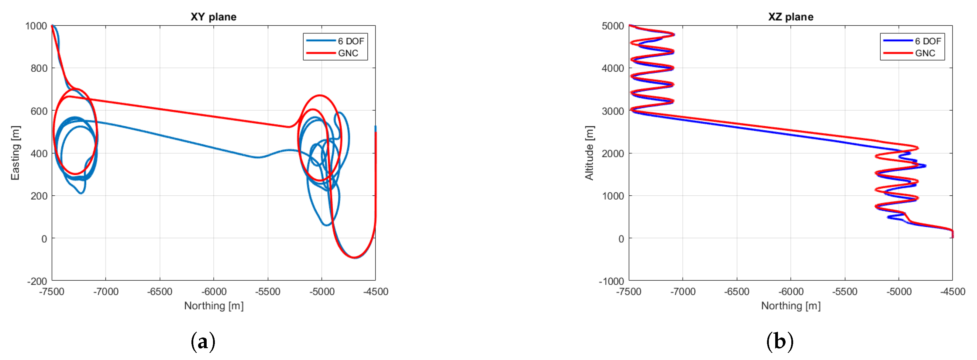
Validation of the Equation of Motions

As mentioned, the model has already been validated in steady-state with some drop tests performed at NASA JPL on a parafoil–payload precision landing system [33]. However, seeing the application with a lifting body as a payload, a second validation round has been performed with reference data provided by TAS-I, specified in the plots by the label “TAS-I”.

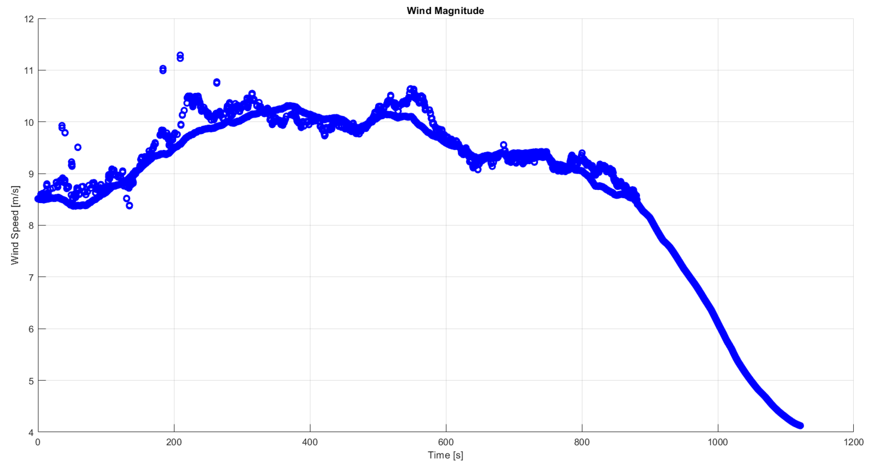
The drop test was performed during a windy day, of which the wind magnitude can be seen in Figure 6. The control deflections, ${\delta }_s$ and ${\delta }_a$, were provided by the TAS-I dataset.The aerodynamic and geometrical parameters were set as the one previously introduced in Section 2.1 and Section 2.2.

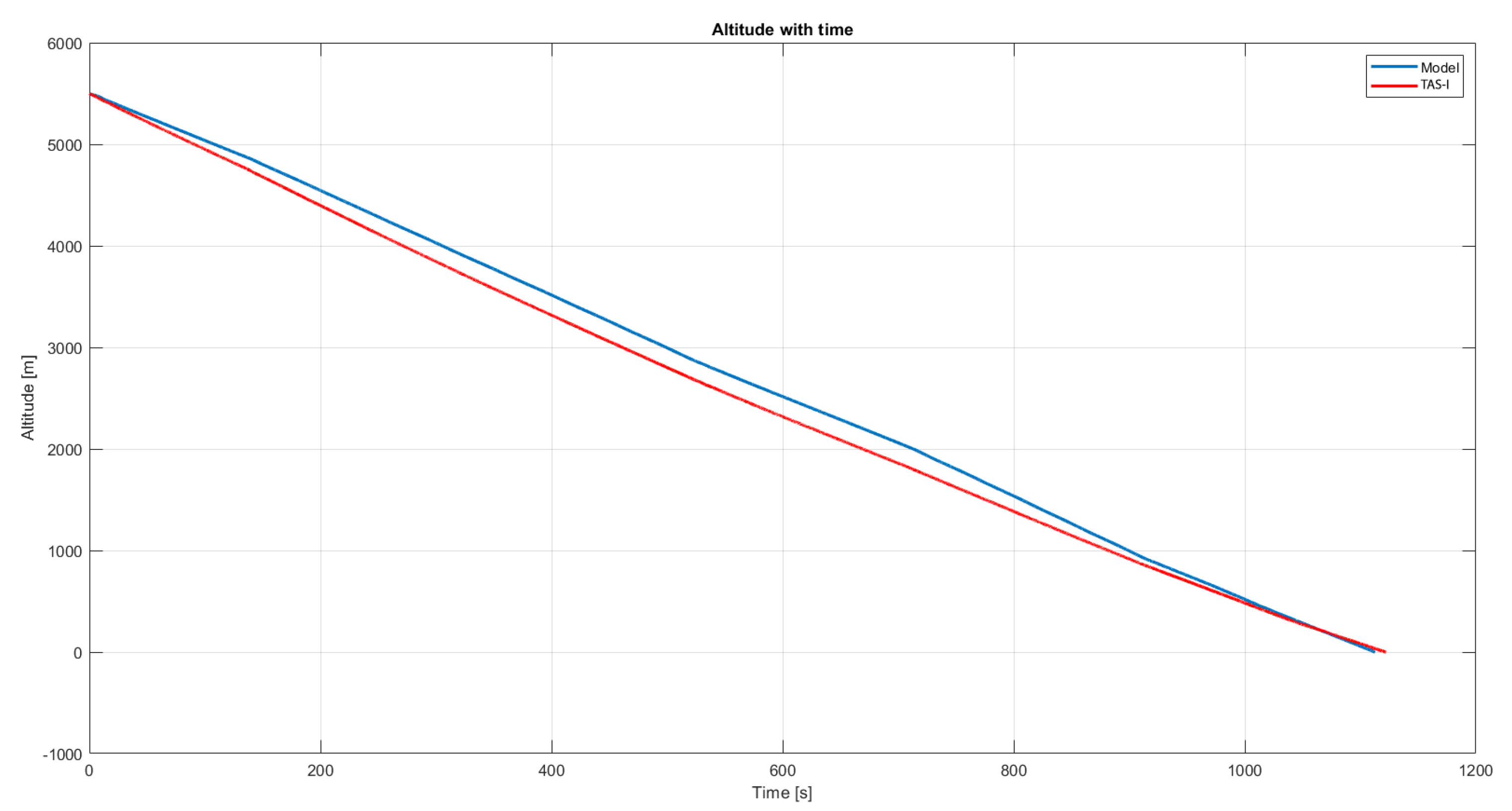
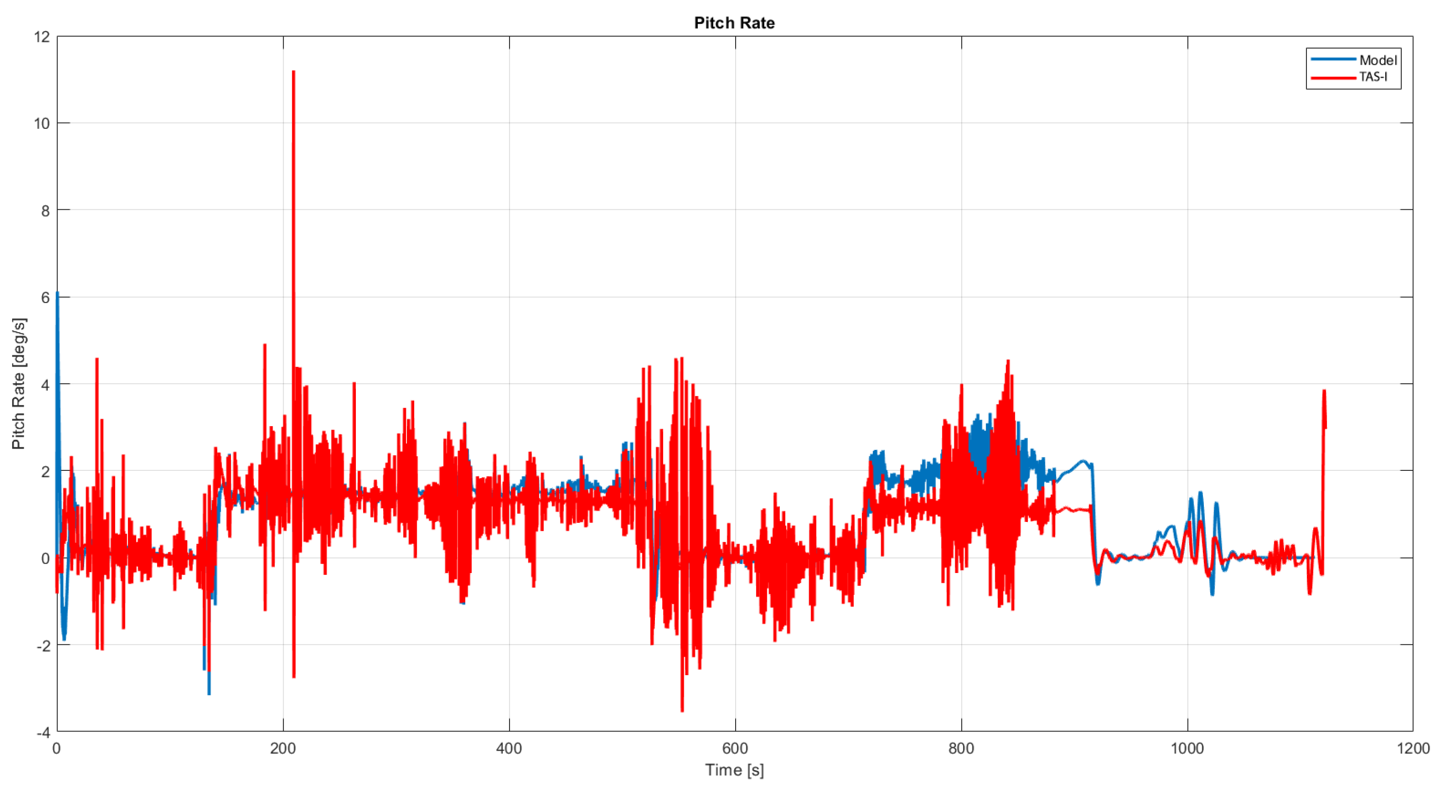
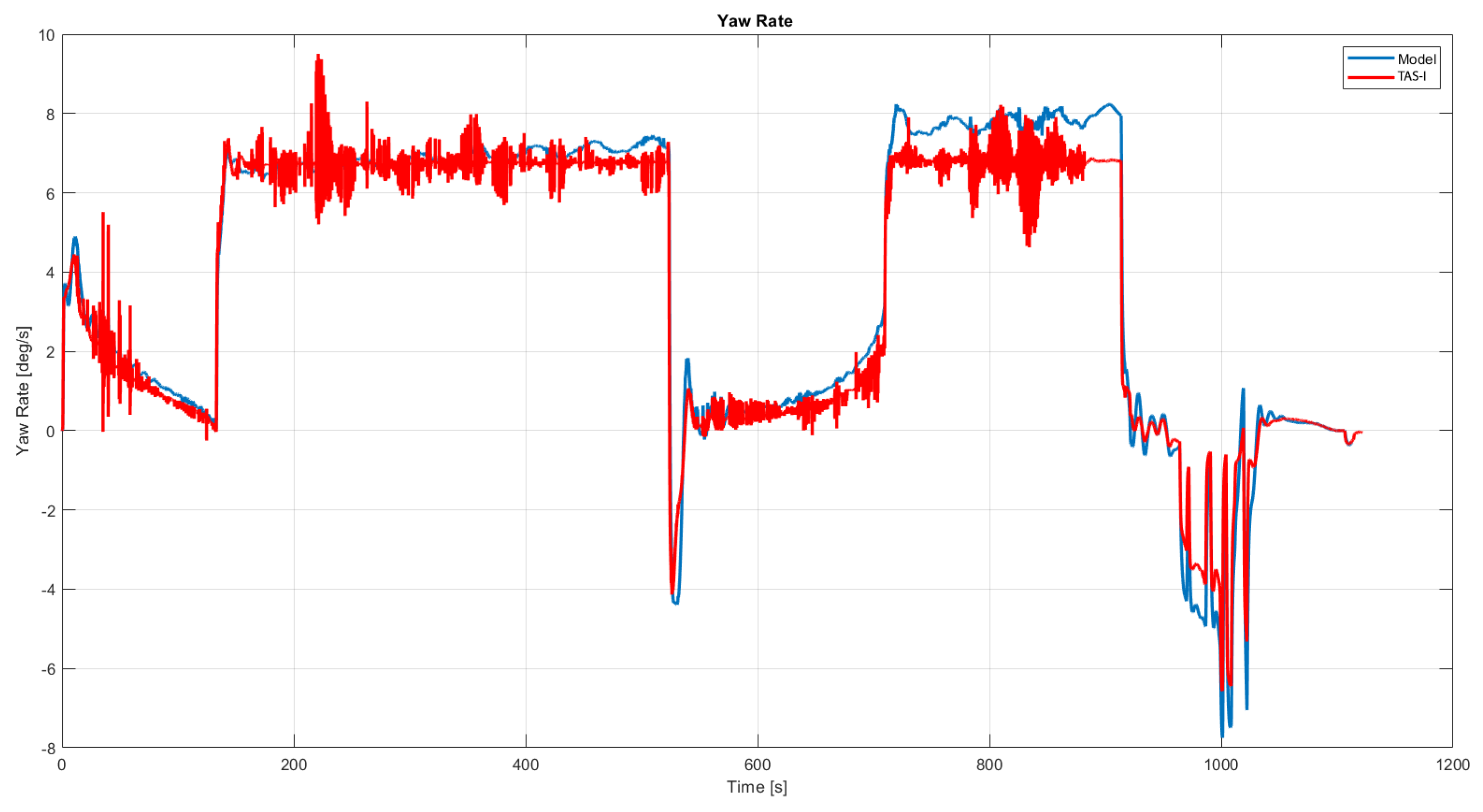
Figure 7 shows the trajectory followed by the parafoil during the drop test as evaluated by the tool. The descent rate difference between the drop-test and the model is presented in Figure 8, while the angular rates are shown in: roll rate in Figure 9, pitch rate in Figure 10 and yaw rate in Figure 11.

Unfortunately, no other quantitative figure of merits has been provided by TAS-I for validation. However, the six DOF model follows the test trends with an error of less than 2%. Therefore, it was considered robust enough to be used as the primary dynamic model in the tool while investigating different solutions.

2.4. Guidance, Navigation and Control

The main innovation point of the presented study lies in the fusion of the sizing, aerodynamics and dynamics modules with a guidance, navigation and control routine. The tool refines the parafoil’s design by assessing the feasibility of a typical landing trajectory, estimating the overall trajectory efficiency, the control depth and landing velocities of the analysed configuration.

In more detail, the GNC module of PIMENTO implements (i) a 3 DOF kino-dynamic model to provide the reference trajectory to the system, (ii) the wind and density estimation during the simulated flight, and (iii) a control logic and saturation to follow the reference trajectory. The following subsections will analyse in detail some of these three aspects.

The navigation module relies on existing density, gust, and wind models [31,36,37]. Therefore, it will not be further detailed. On the other hand, this section will focus on the mathematical formulation of the guidance and control modules.

2.4.1. Guidance Model

The presented trajectory model relies on a three-DOF model. As detailed in [1,15,23], the final approach trajectories are usually based on two spirals: the loiter phase and the energy management phase. They are used to lower the altitude and energy of the system. They are joined by a straight line referred to as homing phase. Finally, a terminal turn is performed to align the system to the target and lower its touchdown velocity with a final flaring manoeuvre [38].

This reference trajectory is the one used in the tool to assess the stability of the studied configuration during turn manoeuvres with or without wind with the six or nine DOF.

During the path definition, the wind vector is assumed to be W = [$W_x$,0,0] [1]. Hence, the wind component along x is assumed to be the strongest constraint to be accommodated while planning the trajectory. Throughout the formulation, the wind is considered in the guidance equations as in [39].

The 3 DOF dynamic model relies on the following assumptions:

• the velocity is constant;
• the heading angle is defined from the geometry of the trajectory and its waypoints;
• the sphericity of the Earth is not considered because the final manoeuvres start around five kilometres from ground [15].

The equations used are expressed in the NED reference system, and they identify the accelerations along the x, y, and z-axis (Equations (19)–(21)), where:

• $V_a$ is the flight path velocity;
• ${\chi }_a$ is the heading angle;
• ${\gamma }_a$ is the flight path angle.

$$\dot{z}=-V_a\ast sin\left({\gamma }_a\right)$$

(19)

$$\dot{y}=-V_a\ast sin\left({\chi }_a\right)\ast cos\left({\gamma }_a\right)$$

(20)

$$\dot{x}=-V_a\ast cos\left({\chi }_a\right)\ast cos\left({\gamma }_a\right)$$

(21)

The guidance model simulates the behaviour of the parafoil following the trajectory geometrically defined in the three main parts:

• Loiter: a spiral around the loiter centre;
• Energy management: a spiral around the energy management centre;
• Final approach: a last turn to align to the dropping point.

Each part is connected with straight lines. The entry in each spiral is joined to the previous straight line with an S-maneuver [27].

The efficiency of the 3 DOF model is fixed during the trajectory study. It is equal to the expected performance in the parafoil flight (the nominal $L/D$). The flight path angle is calculated from the lift over drag ratio. The desired flight path angle (${\gamma }_{des}$) is defined in the whole trajectory, as in Equation (22):

$${\gamma }_{des}=-atan(\frac{1}{C_L/C_D})$$

(22)

The heading angle and the heading rate will change within the trajectory phases to control the directions of the parafoil. In the “straight-lines” parts, the desired heading angle is defined as Equation (23):

$${\chi }_{des}=-atan(\frac{(y_{des}-y)+wy\ast dt}{(x_{des}-x)+wx\ast dt})=-atan(\frac{\Delta y}{\Delta x})$$

(23)

The heading rate is evaluated from the actual heading angle and the desired one difference. However, this value is saturated considering the maximum allowable turn rate of the parafoil for a given efficiency.

During S-maneuver entrance phase [27], the heading rate is defined as in Equation (24):

$${\dot{\chi }}_{des}=V_a\ast cos({\gamma }_a)/R$$

(24)

where the parameter R can be:

• the radius of the spiral, in the loiter and energy management spirals;
• the turn radius of the parafoil during an S-maneuver.

The final approach geometry is derived from [23]. The parafoil follows a straight line, and then it turns about 180 degrees to align itself with the landing point along the x-axis. The overall reference trajectory is shown in Figure 12, Figure 13 and Figure 14.

2.4.2. Control Saturation and Flare Manoeuvre

The PIMENTO simulator implements a proportional control that takes into account the difference in heading between the desired trajectory from the guidance module and the actual trajectory (Equation (25)). The control is then normalized for the maximum allowable deflection, ${\delta }_{max}$ (Figure 3).

The proportional control to follow the trajectory focuses on the latero-directional deflection, ${\delta }_a$. However, the related longitudinal deflection, ${\delta }_s$, can be estimated assuming that one side is always deflected up to the minimum deflection. In contrast, the side of the turn varies its deflection with the control law in Equation (25). The two sides are indicated as ${\delta }_{left}$ and ${\delta }_{right}$.

Both deflections, ${\delta }_a$ and ${\delta }_s$, change the aerodynamic of the parafoil as highlighted in the equations of Section 2.3.

Equations (26) and (27) show the modelling of the symmetric deflection due to the asymmetric deflection. Therefore, they explicit the impact on the longitudinal plane with respect to the turn manoeuvre:

$${\delta }_a=K_p\ast ({\chi }_{desired}-{\chi }_{effective})$$

(25)

$${\delta }_s=({\delta }_{right}+{\delta }_{left})/2$$

(26)

$${\delta }_a=({\delta }_{right}-{\delta }_{left})$$

(27)

The flare manoeuvre is initiated at a limit altitude that the user can set. If no limit altitude is explicit, PIMENTO assumes an initial limit altitude of 8 m derived from the X-38 drop tests [40].

The touchdown limit in the simulator is set to 3 m/s [35], for the vertical velocity. In contrast, the limit for the horizontal velocity has been set around 15 m/s following the same constraints of the X-38 [3]. Those are typical landing constraints to ensure the safety of the payload.

When the limit altitude is reached, the system switches toward the flare configuration and maintains it up to the landing.

A control saturation model limits all the control manoeuvres. Its inputs are the voltage and power associated with the system’s winches, (Equation (28)) and the effort to reach a given deflected position. The efficiency is usually set at $0.8$. The real delta position of the lines at each simulation step is derived in Equation (29). The time step of the control saturation is usually smaller than the simulation time step to have a good approximation of the real system behaviour:

$$P_{eff}=Voltage\ast Current\ast Efficiency$$

(28)

$${\Delta }_{position}=\frac{P_{eff}}{F_{effort}}\ast d{t}_{control}$$

(29)

2.5. Inflation Model

To consider the overall chain of events from parafoil deployment to landing, an inflation model was added to the tool logic.

The inflation models run at the beginning of the PIMENTO routine to define the rates and velocities at parafoil inflation. Different inflation models have been extensively analysed and discussed in [1,41]. Both models consider parafoil inflation as a ballistic phenomenon. The inflation analysis considered in the tool is based on [41]. The results obtained are in good agreement concerning the data provided by TAS-I.

3. Results and Discussion

Section 2 detailed all the PIMENTO modules and their modelling, while Figure 2 shows the connections between these modules. The overall approach builds on some known literature adapted for the given application, such as preliminary sizing rules, inflation, and dynamic models for parafoil. First, it refines the sizing rules using a database from literature data. Next, it defines simple yet realistic algorithms for guidance and control to simulate the landing of the parafoil. Finally, it suggests a method to define the parafoil aerodynamic set, knowing the aspect ratio. These elements combine to create a rapid-prototyping framework where different designs can be iterated in a few minutes.

The end objective of the integrated approach is to understand the design box for an analysed spaceplane’s parafoil. The aim is not an in-depth design, but a preliminary feasibility assessment of parafoil–payload configurations. Then, the most promising solutions will be investigated in detail through a CAD design, CFD analysis and ad-hoc optimal guidance and control simulations.

In general, the tool outputs the positions, attitudes, velocities, angular rates, aerodynamic forces, and the resulting trajectory of the analysed parafoil–payload system.

The case study presented in this paper uses the parameters shown in

Table 2. Main system parameters used for the PIMENTO simulations in this paper.

Parameter	Value
Canopy Area (S)	280 m${}^2$ [35]
Max L/D (L/D: Lift over Draf)	4 [35]
Max turn ratio	10 deg/s [35]
Length lander	4.4 m [42]
Wingspan lander	2.2 m [42]
Height lander	1.5 m [42]
Max touch down velocity	3 m/s [35]
Mass lander	from 2028 kg to 2734 kg [42]

. The missing parameters have been estimated using the mathematical expressions in Table 2 or the database and validated with the reference data provided by TAS-I. On the other hand, the payload aerodynamic coefficients have been retrieved from the Space Rider data [42] and its predecessor systems, the IXV [42] and the PRIDE feasibility study [43].

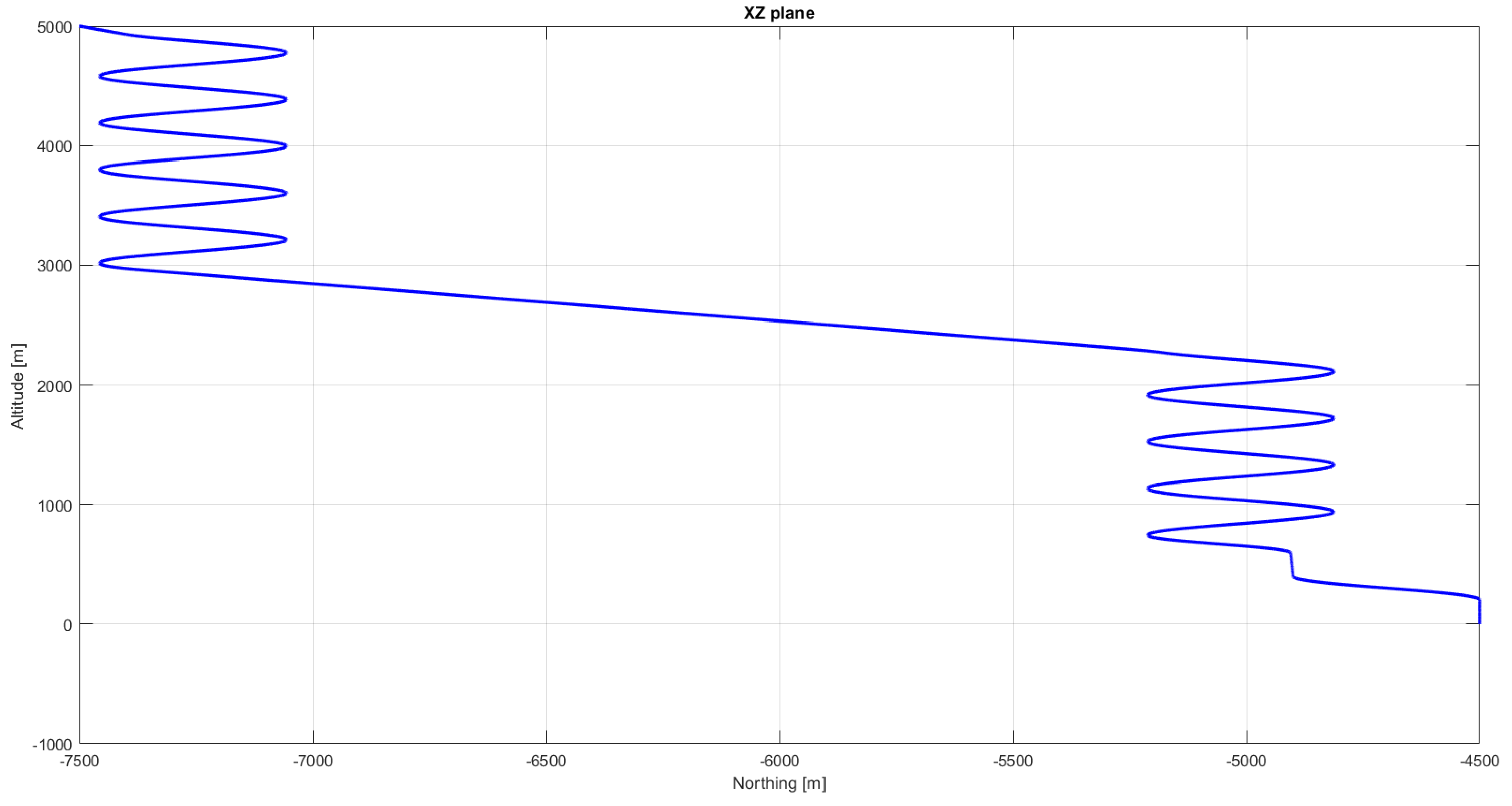
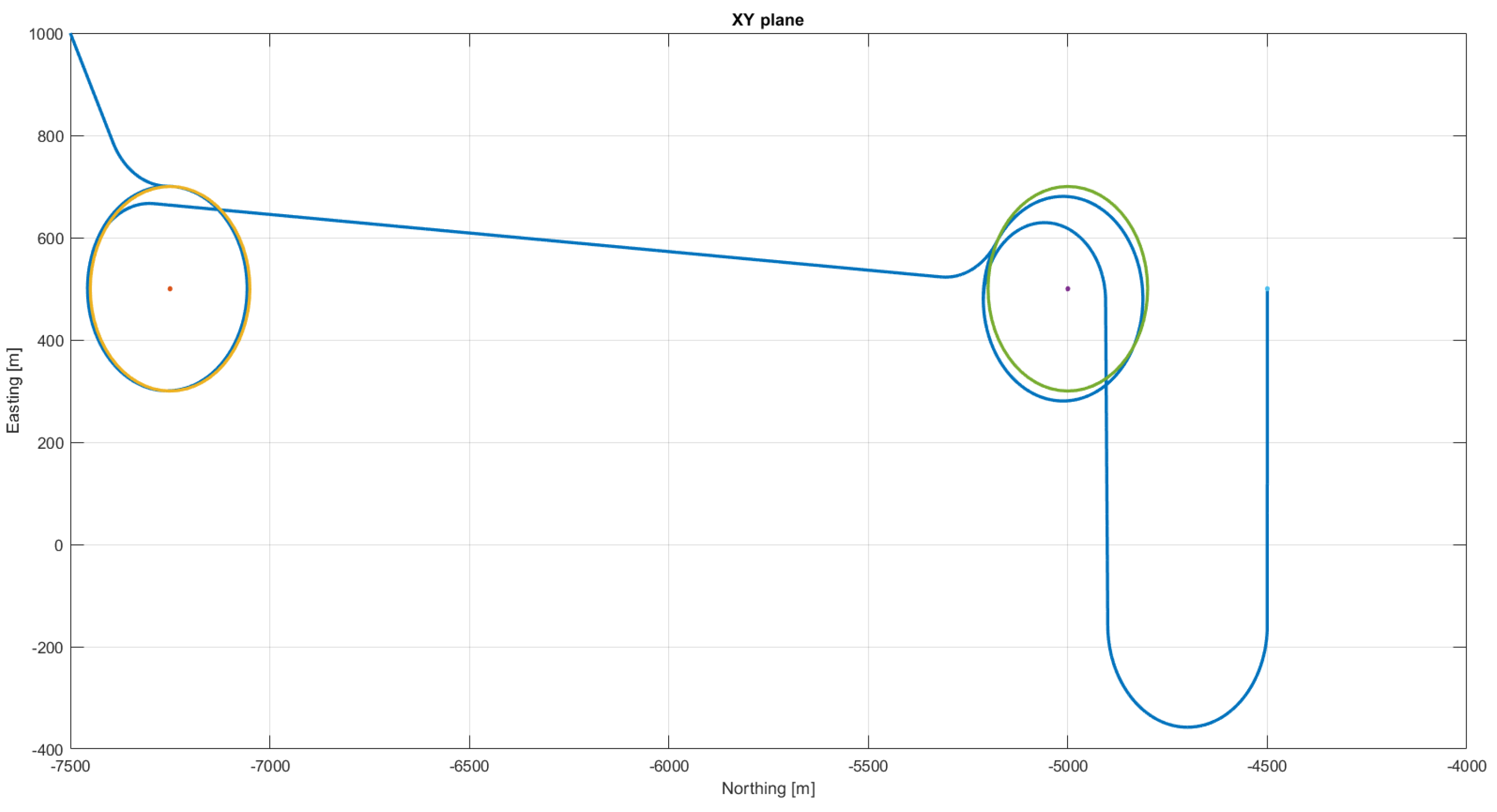
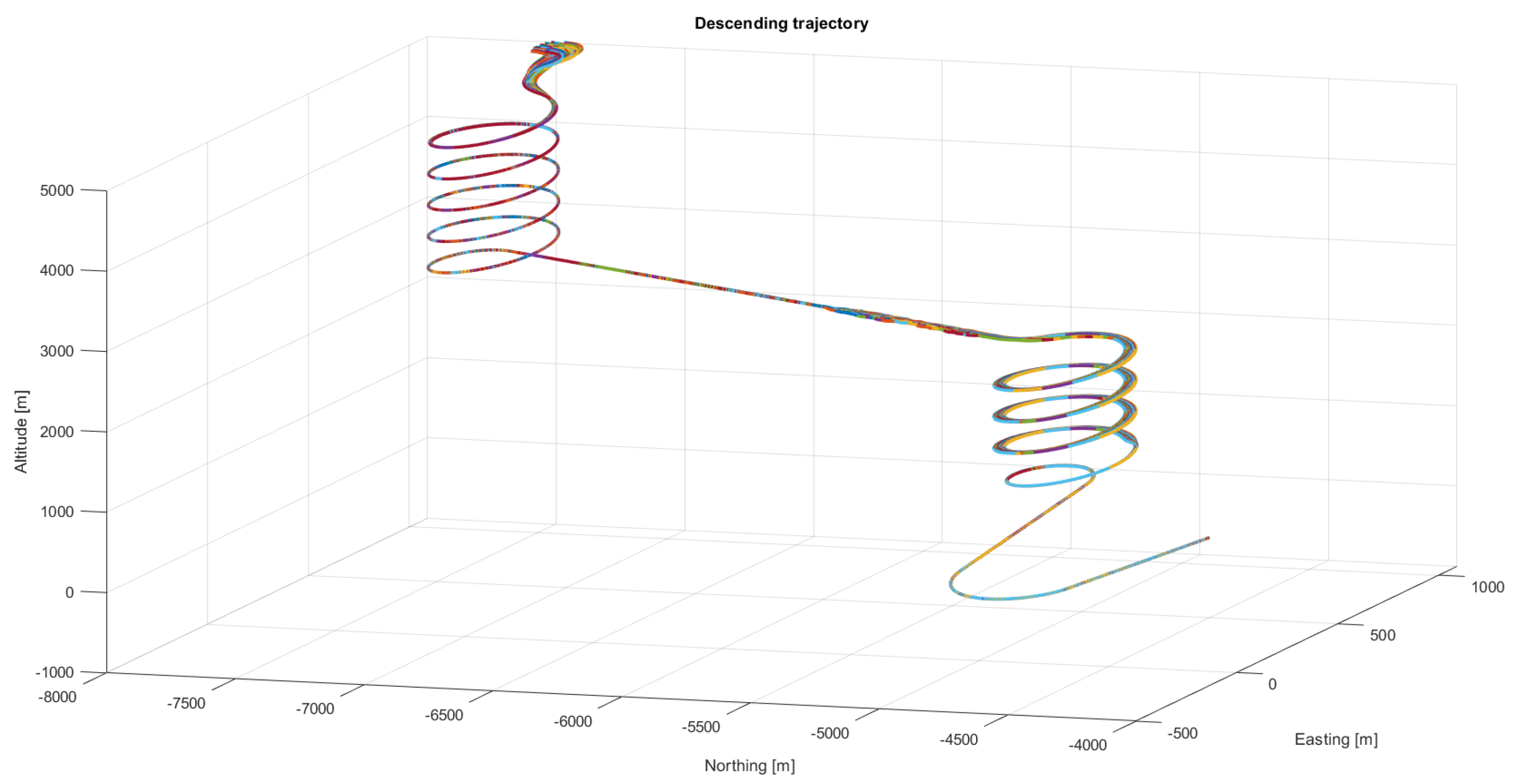
An example of the output trajectory of the 6 DOF model without wind is presented in Figure 15 and Figure 16. The simulation parameters used are the ones presented in Table 2 with a payload of 2028 kg.

Thanks to the parametrization of the geometrical characteristics in PIMENTO, it is easy to automatize different simulations varying the payload mass, the parafoil surface and starting deployment point. For example, the user can quickly analyse the boundaries of different parafoil–payload configurations in terms of vertical mean and landing velocities varying the spaceplane mass as shown in Figure 17. The red strip in Figure 17 highlights the zone where the landing velocity is higher than the maximum allowed one of 3 m/s. The vertical velocity is one of the most indicative figures of merits during preliminary design. It clearly indicates if the given parafoil characteristics are enough to ensure a safe landing to the system. A similar analysis has been conducted, varying the control efficiency for a parafoil of 280 m${}^2$ and a payload of 2028 kg. The results in terms of vertical landing velocity are shown in Figure 18. The variation stops at an efficiency equal to 0.8, the usual control efficiency for parafoils’ winces. During the flight, the parafoil focuses on following the trajectory, not lowering its vertical velocity. Therefore, the mean vertical velocity between the different control efficiency configurations is always around 2.8 m/s, depending only on the parafoil aerodynamic forces and the weight of the parafoil–payload system. On the other hand, the control efficiency affects the landing capabilities of the system during the flare manoeuvre. Analogously, Figure 18 shows the vertical landing velocities for a simulation considering varying current supplies.

Another handy analysis during preliminary design is understanding the position dispersions at touch-down for a given control saturation. In the example of Figure 19, the parafoil is trying to follow the reference trajectory presented in Figure 12. Figure 20a,b show the dispersion at deployment and at touch-down of the different trajectories in Figure 19.

Among the study cases used to verify the tool’s robustness, one focused on assessing the behaviour of the parafoil–payload system in a windy environment. The resulting trajectory is shown in Figure 21, while the partial views of the trajectory are shown in Figure 22. The used wind profile is shown in Figure 23. In the simulation, the parafoil could land 30 m from the expected landing point. This type of simulation can give an insight into how well different configurations withstand wind and if they respect the envisioned landing zone.

Overall, the approach employed in PIMENTO facilitates the parametrization of different types of preliminary simulation easily. Usually, these parametrizations are performed with steady-state simulations. However, PIMENTO provides preliminary modelling of the GNC to start analysing the parafoil–payload landing performances during preliminary design.

4. Conclusions

The paper presents in detail the different modules of the PIMENTO simulator. The starting focus is the geometrical and aerodynamic parameter estimation for parafoils. Then, after defining a feasible aerodynamic database, the six DOF mathematical model behind PIMENTO is detailed and validated with reference data provided by TAS-I. Finally, the guidance, navigation and control module and the inflation module of PIMENTO are introduced. Finally, a set of example results from PIMENTO is briefly introduced and commented on in Section 3.

The presented study points toward the efforts of rapid prototyping of space systems. However, instead of just assessing the dimension of the parafoil for a given weight, the tool focuses on assessing whether the design is effectively feasible for the given application. The proposed dynamic model and GNC architecture are kept simple but effective to understand the landing capabilities of the proposed configurations. Regardless of the end application, when the system engineers start exploring different solutions for spaceplane landings, it is handy to have this type of rapid prototyping tool.

There is still one major open point to be addressed in future works: the aerodynamic modelling. The solution presented in the paper is well adapted to our study case of a lifting body spaceplane. However, it has not been assessed that it is fully generalizable to other applications. Therefore, part of the future works involving PIMENTO would focus on the aerodynamics assessment.

Moreover, the new challenge of designing spaceplanes with parafoil is linked to the aerodynamic interactions between parafoils and the lifting body. This interaction is now modelled through a vector of forces generated by the lifting body. However, future tool developments envision better-integrated parafoil and payload aerodynamic coupling modelling in the six and nine DOF.

The final aim of this ongoing study is to create a reliable, comprehensive, low-fidelity tool to analyse different spaceplane landing configurations.