A New Mapped WENO Method for Hyperbolic Problems

Abstract

In this study, a new family of rational mapping functions g_RM(ω;k,m,s) is introduced for seventh-order WENO schemes. g_RM is a more general family of mapping functions, which includes other mapping functions such as g_M and g_IM as special cases. The mapped WENO scheme WENO-IM(2,0.1), which uses g_IM, performs excellently at fifth order but rather poorly at seventh order. The reason for this loss of accuracy was found to be the over-amplification of very small weights by the mapping process, which can be traced back to the large slope of g_IM at ω = 0. For m > 1, g_RM can be designed to have a unit slope at ω = 0, which will preserve small weights with little to no amplification. It has been demonstrated through several one-dimensional linear advection test cases that the mapped WENO scheme WENO-RM(6,3,2 × 10³), which uses the mapping function g_RM(ω;6,3,2 × 10³), outperforms both WENO-M and WENO-IM(2,0.1) at seventh order. The proposed scheme also performs better at a number of one-dimensional inviscid gas flow problems compared to other popular WENO schemes such as the WENO-Z scheme.

1. Introduction

Hyperbolic problems arise in many scientific and engineering applications. The Euler equations governing the dynamics of an inviscid fluid is a notable example of a non-linear hyperbolic problem which admits discontinuities to develop and persist in the solutions. These discontinuities, such as shock waves and contact surfaces, are key features in high-speed flows and are regularly encountered in aerospace engineering applications [1]. Needless to say, it is imperative to capture these discontinuities accurately. In addition to capturing discontinuities, satisfactory accuracy remains a requirement for smooth flow regions to resolve the finer-scale turbulence as well as pressure and velocity fluctuations, which are essential for the prediction of unsteady aerodynamic behaviour and aerodynamically generated noise [2]. As a result, the development of high-order schemes has attracted significant attention from both aerospace research and engineering communities over the past decade. Conventional high-order schemes, which perform excellently in the smooth regions of the solution, tend to produce spurious oscillations in the vicinity of discontinuities. Harten et al. [3] designed the essentially non-oscillatory (ENO) schemes to overcome this problem by choosing the smoothest stencil to reconstruct the solution, thereby effectively avoiding reconstruction across a discontinuity. Later, Liu et al. [4] proposed the weighted ENO (WENO) scheme in which a weighted reconstruction is obtained from all available stencils, with the weight assigned to each stencil being inversely proportional to the smoothness of the reconstruction within that stencil. In addition to remaining (essentially) non-oscillatory near discontinuities, the WENO method on a (2r − 1)-cell stencil was able to attain the (r +1)th order of convergence in smooth regions, one order higher than the approximations from the constituent r-cell stencils, each of which converge at rth order. Subsequently, Jiang and Shu [5] improved upon the WENO scheme by proposing a new smoothness indicator which allowed the WENO method to achieve the optimal (2r − 1)th order of convergence in smooth regions. This improved scheme is commonly referred to as WENO-JS.

The WENO-JS method has since become a popular choice for solving hyperbolic problems numerically due to its robustness and accuracy. However, a crucial detail remained unnoticed until the work of Henrick et al. [6], which showed that the fifth-order WENO-JS scheme fails to achieve the optimal fifth-order convergence near critical points in the solution where the first derivative of the solution vanished. They explained that the loss of accuracy was masked when a relatively large value such as 10⁻⁶ was used for $ϵ$, a parameter that was thought to be inconsequential and introduced solely to prevent division by zero (see Equation (10)). In addition, they proposed a mapping function g_M to modify the WENO-JS stencil weights to recover the optimal order of accuracy near critical points. This scheme is referred to as WENO-M. More recently, it was shown that g_M actually belongs to a more general family of functions g_IM [7]. Using a different set of parameters, Feng et al. [7] showed that vastly superior results could be obtained for fifth-order WENO. Interestingly, this improved scheme, referred to as WENO-IM(2,0.1), was able to capture discontinuities with very little dissipation compared to WENO-M and WENO-JS. However, when applied to a seventh-order WENO scheme, it was reported to perform poorly [7]. There have been attempts to improve the performance of a WENO-JS scheme that involves modifying the linear weights. Martín et al. [8], for instance, proposed a bandwidth-optimised WENO scheme with a different set of linear weights for improved spectral properties. However, it is likely that such methods also suffer from the same pitfall as the WENO-JS scheme near critical points since the non-linear stencil weights are computed in an identical manner. Mapped WENO methods can likely be applied in conjunction with such methods as well to provide further improvements.

Indeed, high-order WENO schemes are considered appropriate for numerical simulations of high-speed flow scenarios, which require both the ability to capture discontinuities and resolve fine-scale turbulence [9]. Shen and Zha [10] developed a robust seventh-order WENO for a transonic convergent–divergent nozzle and RAE aerofoils. Min [11] implemented a hybrid numerical scheme based on seventh-order WENO for improving the numerical accuracy over a range of 2D and 3D unsteady aerodynamic problems. Sun et al. [4] studied the blade–vortex interaction noise using a seventh-order WENO-Z scheme and concluded that the higher-order scheme was computationally cheaperthan the lower-order schemes with comparable solution accuracy. More recently, Han et al. [12] resolved the helicopter wake flow during hover flight using seventh-order WENO-K scheme and obtained excellent agreement with the measured data at both subsonic and transonic flow regimes. Clearly, high-order WENO schemes are constantly adopted and implemented for improved solution accuracies in various flow problems relevant to aerospace engineering applications.

In this study, the performances of the mapped methods near discontinuities are analyzed for fifth- and seventh-order WENO schemes. In particular, the cause behind the poor performance of the seventh-order WENO-IM(2,0.1) scheme is studied in detail. Based on the insights gleaned, a new family of rational mapping functions is introduced, which, incidentally, includes the mapping functions g_IM as a special case.

This paper is organised as follows: In Section 2, a brief review of WENO-JS and the mapped WENO schemes is provided. Next, in Section 3, the new family of rational mapping functions g_RM(ω;k,m,s) is introduced and a parametric study is performed to determine suitable coefficients k, m and s. In Section 4, the proposed mapped WENO method, WENO-RM(k,m,s), is compared with existing WENO schemes for several linear advection and Euler cases to demonstrate the superior performance of the new method. Finally, the concluding remarks are provided in Section 5.

2. Numerical Methods

2.1. WENO-JS Scheme

To begin with, consider a one-dimensional domain $x\in \left[a,b\right]$ discretized into N cells of width $\Delta x=\left(b-a\right)/N$. The center and interface locations of the ith cell are denoted by x_i and $x_{i\pm 1/2}=x_i\pm \Delta x/2$, respectively. In the finite volume methodology, the discrete solution to a problem is determined in terms of cell averages. Given a function u(x), the ith cell average is denoted by $\overline{u_i}$. In this section, the left-biased fifth- and seventh-order WENO-JS approximations to the point value $u_{i+1/2}^L=\underset{x\to x_{i+1/2}^{-}}{\lim }u\left(x\right)$ are briefly outlined. The stencils for the fifth- and seventh-order reconstructions are shown in Figure 1.

The WENO-JS procedure first computes the r^th order approximations to $u_{i+1/2}^L$ as:

$$u_{i+1/2}^L={\left({\widehat{u}}_{i+1/2}^{L,r}\right)}_j+O\left(\Delta x^r\right)\hspace{1em}j\in \left[0,r-1\right].$$

(1)

For the fifth-order WENO-JS scheme (r = 3), three third order approximations are obtained using the expressions:

$$\begin{array}{l}{\left({\widehat{u}}_{i+1/2}^{L,3}\right)}_0=\frac{1}{6}\left(2\overline{u_{i-2}}-7\overline{u_{i-1}}+11\overline{u_i}\right),\hfill \\ {\left({\widehat{u}}_{i+1/2}^{L,3}\right)}_1=\frac{1}{6}\left(-\overline{u_{i-1}}+5\overline{u_i}+2\overline{u_{i+1}}\right),\hfill \\ {\left({\widehat{u}}_{i+1/2}^{L,3}\right)}_2=\frac{1}{6}\left(2\overline{u_i}+5\overline{u_{i+1}}-\overline{u_{i+2}}\right).\hfill \end{array}$$

(2)

Similarly, for the seventh-order WENO-JS scheme (r = 4), four fourth-order approximations are obtained using the expressions:

$$\begin{array}{l}{\left({\widehat{u}}_{i+1/2}^{L,4}\right)}_0=\frac{1}{12}\left(-3\overline{u_{i-3}}+13\overline{u_{i-2}}-23\overline{u_{i-1}}+25\overline{u_i}\right),\hfill \\ {\left({\widehat{u}}_{i+1/2}^{L,4}\right)}_1=\frac{1}{12}\left(\overline{u_{i-2}}-5\overline{u_{i-1}}+13\overline{u_i}+3\overline{u_{i+1}}\right),\hfill \\ {\left({\widehat{u}}_{i+1/2}^{L,4}\right)}_2=\frac{1}{12}\left(-\overline{u_{i-1}}+7\overline{u_i}+7\overline{u_{i+1}}-\overline{u_{i+2}}\right),\hfill \\ {\left({\widehat{u}}_{i+1/2}^{L,4}\right)}_3=\frac{1}{12}\left(3\overline{u_{i-1}}+13\overline{u_i}-5\overline{u_{i+1}}+\overline{u_{i+2}}\right).\hfill \end{array}$$

(3)

By performing a weighted average of these rth order approximations using the optimal weights $d_j^{\left(r\right)}$, it is possible to obtain the (2r – 1)th order upstream central approximation $u_{i+1/2}^{L,C\left(2r-1\right)}$ as:

$$u_{i+1/2}^{L,C\left(2r-1\right)}={\displaystyle \sum _{j=0}^{r-1}{d}_j^{\left(r\right)}{\left({\widehat{u}}_{i+1/2}^{L,r}\right)}_j}.$$

(4)

The optimal weights for fifth- and seventh-order WENO-JS schemes are given in Equations (5) and (6), respectively.

$$d_0^{\left(3\right)}=\frac{1}{10},\hspace{1em}{d}_1^{\left(3\right)}=\frac{6}{10},\hspace{1em}{d}_2^{\left(3\right)}=\frac{3}{10}$$

(5)

$$d_0^{\left(4\right)}=\frac{1}{35},\hspace{1em}{d}_1^{\left(4\right)}=\frac{12}{35},\hspace{1em}{d}_2^{\left(4\right)}=\frac{18}{35},\hspace{1em}{d}_3^{\left(4\right)}=\frac{4}{35}$$

(6)

For each rth order approximation, a corresponding smoothness indicator is computed. Following Ref. [5], the rth order smoothness indicator $I{S}_j^{\left(r\right)}$ is defined as:

$$I{S}_j^{\left(r\right)}={\displaystyle \sum _{l=1}^{r-1}\Delta x^{2l-1}{\displaystyle {\int }_{x_{i-1/2}}^{x_{i+1/2}}{\left[\frac{d^l{p}_j\left(x\right)}{d{x}^l}\right]}^{2}dx}},$$

(7)

where $p_j\left(x\right)$ refers to the rth order polynomial reconstructed on the jth stencil, which extends from cell (i + j – r +1) to cell (i + j). The explicit forms of $I{S}_j^{\left(r\right)}$ are given for r = 3 and r = 4 in Equations (8) and (9), respectively.

$$\begin{array}{l}I{S}_0^{\left(3\right)}=\frac{1}{4}{\left(\overline{u_{i-2}}-4\overline{u_{i-1}}+3\overline{u_i}\right)}^2+\frac{13}{12}{\left(\overline{u_{i-2}}-2\overline{u_{i-1}}+\overline{u_i}\right)}^2\\ I{S}_1^{\left(3\right)}=\frac{1}{4}{\left(\overline{u_{i-1}}-\overline{u_{i+1}}\right)}^2+\frac{13}{12}{\left(\overline{u_{i-1}}-2\overline{u_i}+\overline{u_{i+1}}\right)}^2\\ I{S}_2^{\left(3\right)}=\frac{1}{4}{\left(3\overline{u_i}-4\overline{u_{i+1}}+\overline{u_{i+2}}\right)}^2+\frac{13}{12}{\left(\overline{u_i}-2\overline{u_{i+1}}+\overline{u_{i+2}}\right)}^2\end{array}$$

(8)

$$\begin{array}{l}I{S}_0^{\left(4\right)}={\left(\frac{1}{3}\overline{u_{i-3}}-\frac{3}{2}\overline{u_{i-2}}+3\overline{u_{i-1}}-\frac{11}{6}\overline{u_i}\right)}^2+\frac{13}{12}{\left(\overline{u_{i-3}}-4\overline{u_{i-2}}+5\overline{u_{i-1}}-2\overline{u_i}\right)}^2\\ \hspace{1em}\hspace{1em}+\frac{781}{720}{\left(\overline{u_{i-3}}-3\overline{u_{i-2}}+3\overline{u_{i-1}}-\overline{u_i}\right)}^2\\ I{S}_1^{\left(4\right)}={\left(\frac{1}{6}\overline{u_{i-2}}-\overline{u_{i-1}}+\frac{1}{2}\overline{u_i}+\frac{1}{3}\overline{u_{i+1}}\right)}^2+\frac{13}{12}{\left(\overline{u_{i-1}}-2\overline{u_i}+\overline{u_{i+1}}\right)}^2\\ \hspace{1em}\hspace{1em}+\frac{781}{720}{\left(\overline{u_{i-2}}-3\overline{u_{i-1}}+3\overline{u_i}-\overline{u_{i+1}}\right)}^2\\ I{S}_2^{\left(4\right)}={\left(\frac{1}{3}\overline{u_{i-1}}+\frac{1}{2}\overline{u_i}-\overline{u_{i+1}}+\frac{1}{6}\overline{u_{i+2}}\right)}^2+\frac{13}{12}{\left(\overline{u_{i-1}}-2\overline{u_i}+\overline{u_{i+1}}\right)}^2\\ \hspace{1em}\hspace{1em}+\frac{781}{720}{\left(\overline{u_{i-1}}-3\overline{u_i}+3\overline{u_{i+1}}-\overline{u_{i+2}}\right)}^2\\ I{S}_3^{\left(4\right)}={\left(\frac{11}{6}\overline{u_i}-3\overline{u_{i+1}}+\frac{3}{2}\overline{u_{i+2}}-\frac{1}{3}\overline{u_{i+3}}\right)}^2+\frac{13}{12}{\left(2\overline{u_i}-5\overline{u_{i+1}}+4\overline{u_{i+2}}-\overline{u_{i+3}}\right)}^2\\ \hspace{1em}\hspace{1em}+\frac{781}{720}{\left(\overline{u_i}-3\overline{u_{i+1}}+3\overline{u_{i+2}}-\overline{u_{i+3}}\right)}^2\end{array}$$

(9)

With the smoothness indicators computed, the non-linear WENO-JS stencil weights ω_j can be computed as

$${\alpha }_j=\frac{d_j}{{\left(I{S}_j+ϵ\right)}^2},\hspace{1em}{\omega }_j=\frac{{\alpha }_j}{{\displaystyle \sum _{j=0}^{r-1}{\alpha }_j}}.$$

(10)

The superscript (r) will be dropped for the sake of conciseness. The value of $ϵ$ is taken to be 10⁻⁶ for WENO-JS scheme and 10⁻⁴⁰ for all the mapped WENO schemes, as recommended in Ref. [6]. Finally, the (2r −1)th order WENO-JS approximation $u_{i+1/2}^{L,W}$ is obtained by taking a weighted average of the rth order approximations using ω_j, as shown in Equation (11).

$$u_{i+1/2}^{L,W}={\displaystyle \sum _{j=0}^{r-1}{\omega }_j{\left({\widehat{u}}_{i+1/2}^L\right)}_j}$$

(11)

2.2. Mapped WENO Schemes

In order for the WENO approximation in Equation (11) to converge at the optimal (2r −1)th order in smooth regions, ω_j has to satisfy the criterion

$${\omega }_j-d_j=O\left(\Delta x^{r-1}\right).$$

(12)

This holds true for all values of r. However, the WENO-JS scheme does not satisfy this criterion near critical points. A critical point is defined as a point where one or more derivatives of the function u(x) vanish. At a critical point x = x_c of order n_cp (i.e., a critical point of nth order), the first n_cp derivatives of the function u(x) vanish, i.e., $u^{\prime }\left(x_c\right)=\cdots$$=u^{\left(n_{cp}\right)}\left(x_c\right)=0$. It can be shown that the WENO-JS approximation exhibits the convergence behaviour

$${\omega }_j-d_j=O\left(\Delta x^{r-1-n_{cp}}\right),$$

(13)

for $n_{cp}=1,\cdots ,r-1$ instead of that in Equation (12) [7]. Thus, when no derivatives vanish (n_cp = 0), WENO-JS approximation converges at optimal order, whereas the order of convergence deteriorates as n_cp increases.

In order to restore the order of convergence, and, hence, the accuracy near critical points, Henrick et al. [6] suggested the use of a mapping function g(ω) with the following properties:

(a)

$g\left(0\right)=0$, $g\left(d\right)=d$ and $g\left(1\right)=1$;

(b)

Monotone increasing with finite slopes for $\omega \in \left[0,1\right]$;

(c)

$g^{\prime }\left(d\right)=\cdots =g^{\left(k\right)}\left(d\right)=0\ne g^{\left(k+1\right)}\left(d\right)$, i.e., the function flattens near $\omega =d$.

The mapping function g(ω) can be used to calculate the mapped weights ${\tilde{\omega }}_j$ from the WENO-JS weights ω_j obtained from Equation (10), as shown in Equation (14). The mapped WENO approximation of $u_{i+1/2}^L$ is obtained by replacing ω_j in Equation (11) with the mapped weights

$${\tilde{\omega }}_j=\frac{g\left({\omega }_j\right)}{{\displaystyle \sum _{j=0}^{r-1}g\left({\omega }_j\right)}}.$$

(14)

Following their analyses, the mapping function g(ω) can be expanded using Taylor series about ω_j = d_j to demonstrate that the mapping process is indeed able to recover the optimal order of accuracy near critical points.

$$g\left({\omega }_j\right)=g\left(d_j\right)+{\displaystyle \sum _{l=1}^k\frac{1}{l!}{g}^{\left(l\right)}\left(d_j\right){\left({\omega }_j-d_j\right)}^l}+\frac{1}{\left(k+1\right)!}{g}^{\left(k+1\right)}\left(d_j\right){\left({\omega }_j-d_j\right)}^{k+1}+\cdots$$

(15)

Equation (15) can be simplified using the properties of the mapping function mentioned earlier. From property (a), g(d_j) = d_j, and all the terms inside the summation vanish due to property (c). Finally, substituting Equation (13) into the result and rearranging yields

$$g\left({\omega }_j\right)=d_j+\frac{1}{\left(k+1\right)!}{g}^{\left(k+1\right)}\left(d_j\right){\left({\omega }_j-d_j\right)}^{k+1}+\cdots =d_j+O\left(\Delta x^{\left(k+1\right)\left(r-1-n_{cp}\right)}\right).$$

(16)

Substituting Equation (16) into Equation (14) and using the fact that d_j sum to unity, results in

$${\tilde{\omega }}_j-d_j=O\left(\Delta x^{\left(k+1\right)\left(r-1-n_{cp}\right)}\right).$$

(17)

Comparing Equation (17) with Equation (12), it can be concluded that as long as $\left(k+1\right)\left(r-1-n_{cp}\right)\ge r-1$, the mapped weights ${\tilde{\omega }}_j$ satisfy the required criterion. For example, for fifth-order convergence at a critical point of order n_cp = 1, k must be equal to or greater than 1.

The mapping functions put forward by Henrick et al. [6] and Feng et al. [7] denoted by g_M(ω) and g_IM(ω;k,A), respectively, are given in Equations (18) and (19) as a reference prior to introducing the proposed mapping function in the present study.

$$g_{\mathrm{M}}\left(\omega \right)=\frac{\omega \left(d+d^2-3d\omega +{\omega }^2\right)}{d^2+\left(1-2d\right)\omega }$$

(18)

$$g_{\mathrm{IM}}\left(\omega ;k,A\right)=d+\frac{A{\left(\omega -d\right)}^{k+1}}{A{\left(\omega -d\right)}^k+\omega \left(1-\omega \right)}$$

(19)

In the function g_IM(ω;k,A), k is a positive even integer and A is a positive real number. It can be shown directly that $g_{\mathrm{M}}\left(\omega \right)=g_{\mathrm{IM}}\left(\omega ;2,1\right)$, i.e., g_M belongs to the g_IM family of functions. Moreover, the g_IM family of functions satisfies all the properties (a)–(c) mentioned earlier.

Feng et al. [7] showed that $g_{\mathrm{IM}}\left(\omega ;2,0.1\right)$ vastly outperforms g_M(ω) (i.e., $g_{\mathrm{IM}}\left(\omega ;2,1\right)$) for fifth-order WENO schemes. Both the mapping functions are shown in Figure 2 for the smallest and largest values of the optimal weights $d_j^{\left(r\right)}$ for r = 3 and r = 4. Notice that $g_{\mathrm{IM}}\left(\omega ;2,0.1\right)$ is much flatter than g_M(ω) near ω_j = d_j, signifying that $g_{\mathrm{IM}}\left(\omega ;2,0.1\right)$ attempts to map a wider range of weights in the neighbourhood of ω_j = d_j to the optimal weight d_j. As a result, $g_{\mathrm{IM}}\left(\omega ;2,0.1\right)$ is quicker to bring the mapped weights ${\tilde{\omega }}_j$ close to the optimal weights d_j compared to g_M(ω).

3. A New Family of Mapping Functions

3.1. Motivation

Consider the one-dimensional linear advection problem

$$\frac{\partial u}{\partial t}+\frac{\partial u}{\partial x}=0,$$

(20)

which represents one of the most straightforward hyperbolic problems. Given the initial condition $u\left(x,t=0\right)=u_0\left(x\right)$, its exact solution is simply $u\left(x,t\right)=u_0\left(x-t\right)$, which makes it a suitable starting point for the assessment of numerical schemes. It must be remarked that the Euler equations reduce to linear advection of density in the absence of velocity and pressure gradients.

Averaging Equation (20) over the ith cell results in the ordinary differential equation (ODE) for the cell average ${\overline{u}}_i$

$$\frac{d{\overline{u}}_i}{dt}=-\frac{1}{\Delta x}\left(u_{i+1/2}^L-u_{i-1/2}^L\right).$$

(21)

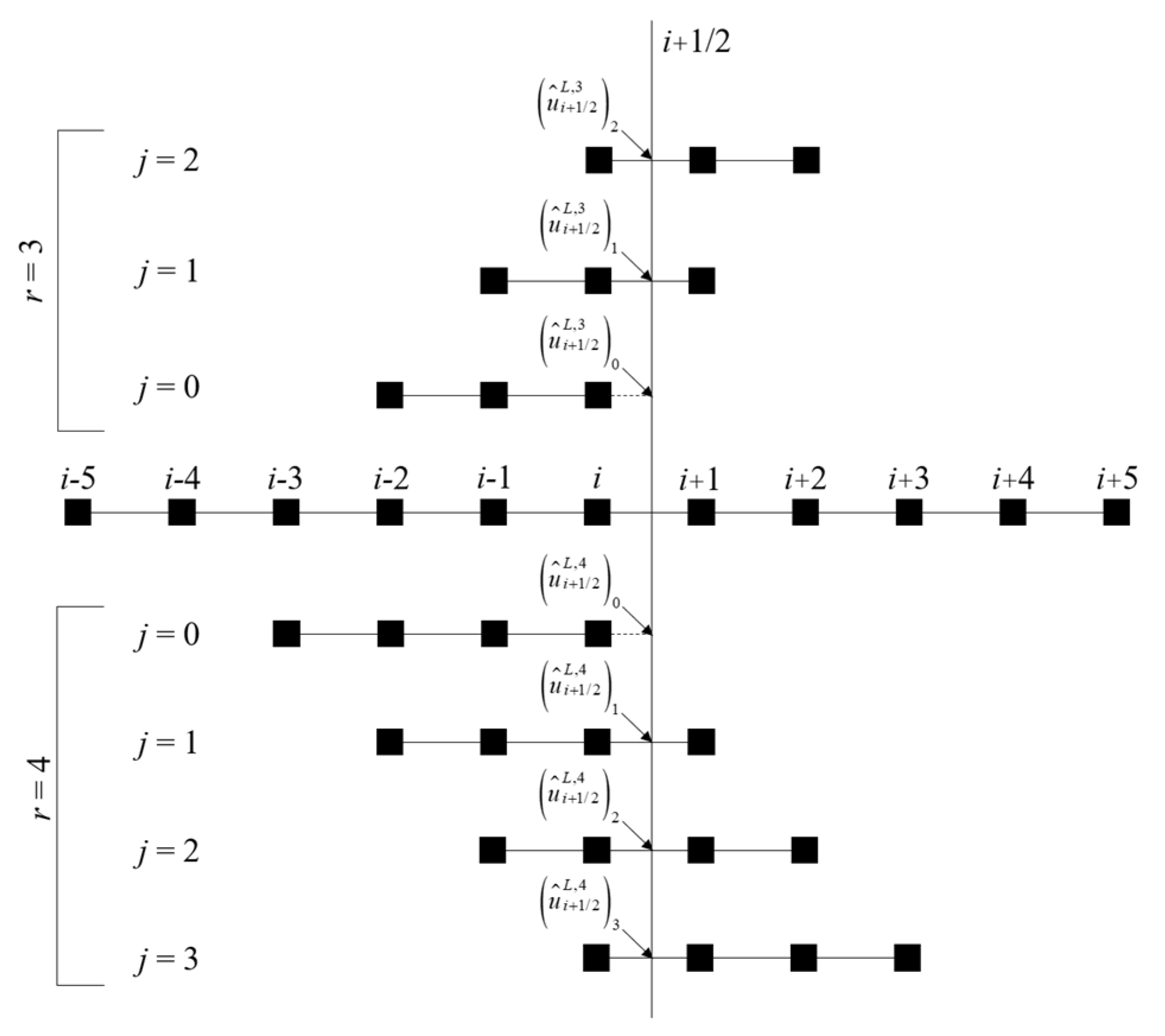
Notice that the right-hand side of Equation (21) involves the left-biased approximations of u(x) at the cell interfaces, which can be obtained through the WENO schemes described in the previous sections. In the present study, this ODE was solved in time using the explicit third-order TVD Runge–Kutta time-marching scheme [13].

With the numerical schemes defined, consider the initial condition of two constant states separated by discontinuities at x = 0 and x = ±0.5

$$Case A1 {\overline{u}}_i=\{\begin{array}{cc}+1,& -0.5\le x_i<0\\ -1,& 0\le x_i\le 0.5\end{array}.$$

(22)

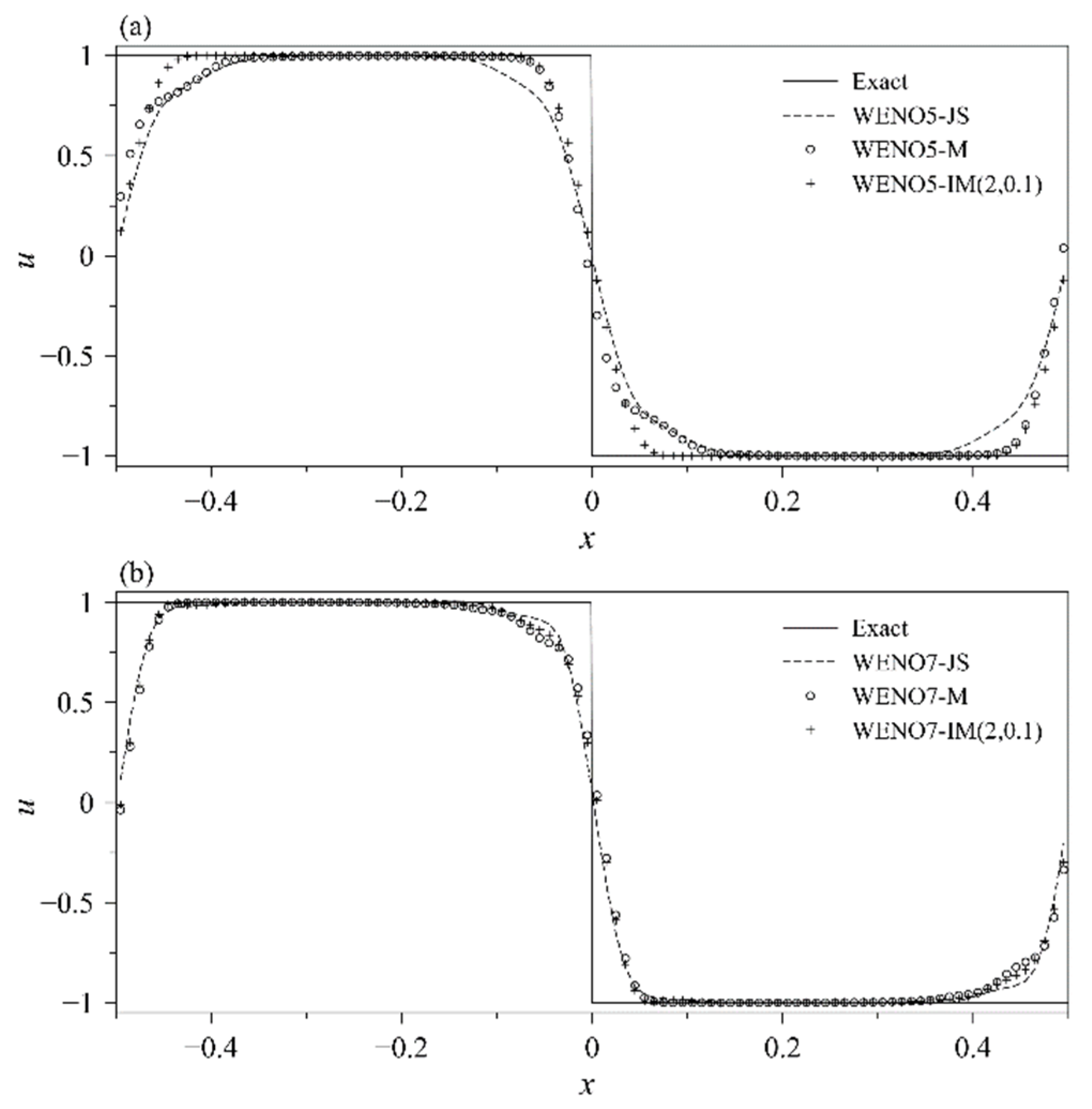
This problem was solved on the periodic domain $x\in \left[-0.5,0.5\right]$ discretized into N = 100 uniform cells using fifth- and seventh-order WENO schemes until t = 100 s (100 cycles) using CFL = 0.1. Note that the mapped WENO methods using g_M(ω) and $g_{\mathrm{IM}}\left(\omega ;2,0.1\right)$ are denoted by WENO-M and WENO-IM(2,0.1), respectively. The final profiles are shown in Figure 3.

It can be observed from Figure 3a that at fifth order, the mapped WENO schemes WENO-M and WENO-IM(2,0.1) are able to capture the discontinuities with lesser numerical diffusion compared to the WENO-JS scheme. Recall that mapped WENO methods were developed to achieve optimal accuracy near smooth critical points. Yet, they seem to be able to capture sharper discontinuities than the original unmapped WENO-JS scheme. Between the mapped WENO schemes, WENO-IM(2,0.1) performs better as it captures the flat regions on both sides of the discontinuities more accurately. In contrast, WENO-M suffers a loss of accuracy to the right of the discontinuities and performs similar to WENO-JS scheme. On the other hand, the results become different at seventh order, as seen from Figure 3b. Both the mapped WENO schemes deliver a similar, and at some regions even worse, performance compared to WENO-JS scheme. This can be determinantal when simulating the propagation of discontinuities and sharp gradients over long distances.

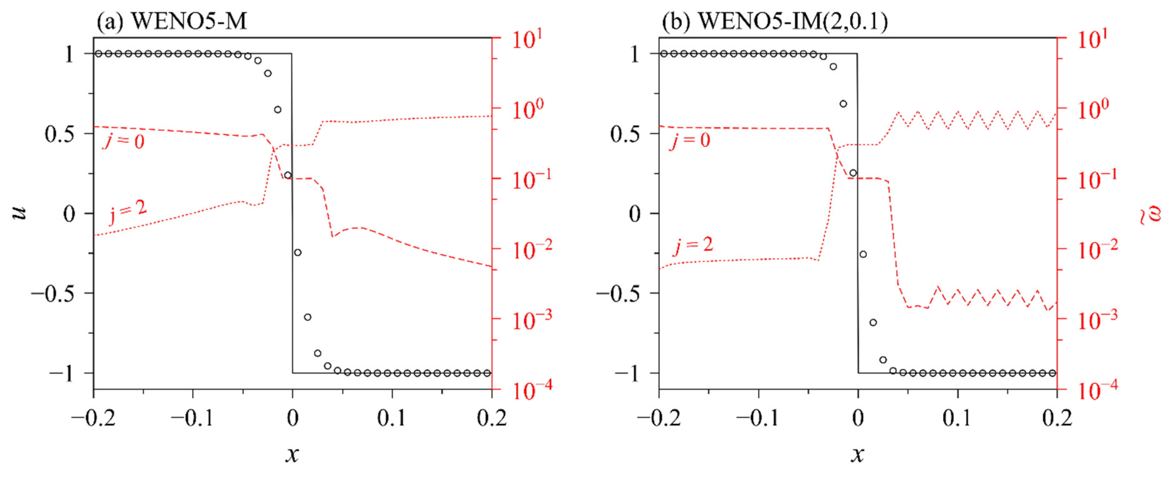
WENO-M and WENO-IM(2,0.1) both suffer a particularly significant loss in accuracy at the flat regions slightly to the left of the discontinuities. To better understand this loss in accuracy, the mapped weights were analysed in detail. The mapped weights ${\tilde{\omega }}_j$ of the leftmost and rightmost stencils, i.e., j = 0 and j = 2, at the end of the first cycle (t = 1 s) are plotted for fifth-order WENO-M and WENO-IM(2,0.1) schemes in Figure 4. Comparing Figure 4a,b, a common trend can be discerned—the leftmost stencil weight ${\tilde{\omega }}_0$ is larger than the rightmost stencil weight ${\tilde{\omega }}_2$ in the region to the left of the discontinuity and vice versa to the right. Although the regions on either side of the discontinuity appear smooth and uniform, they are in fact highly non-smooth in the sense that the “flatness” of the profile changes vastly between one stencil to the next. This results in the smoothness indicators IS_j of adjacent stencils being an order of magnitude apart or more. Since a single WENO reconstruction involves multiple stencils (three for fifth order, four for seventh order), the resulting minimum and maximum values of IS_j are several orders of magnitudes apart. This explains the behaviour of the weights mentioned earlier. Interestingly, across the discontinuity itself, the weights remain close to the optimal weights d_j since the discontinuity has been sufficiently “smoothened” by numerical diffusion.

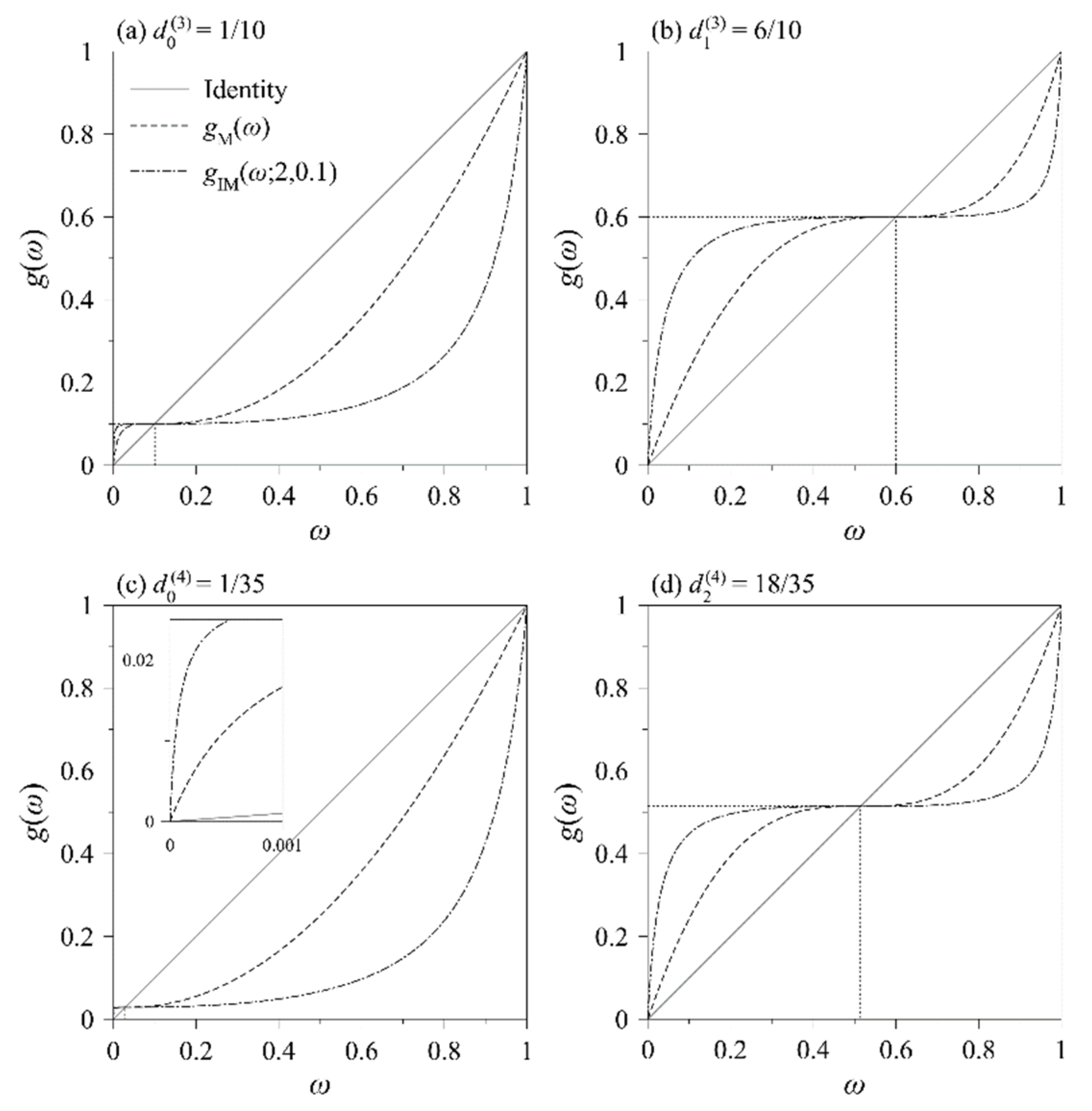
A close examination of the weights near discontinuities suggests that the fifth-order WENO-IM(2,0.1) scheme allocates smaller weights to the non-smooth stencils (j = 2 and j = 0 to the left and right of the discontinuity, respectively) than the fifth-order WENO-M scheme at the end of first cycle, as shown in Figure 4a,b. This is quite unexpected since WENO-IM(2,0.1) scheme generally allocates greater weights to non-smooth stencils than WENO-M scheme, as evident from the shapes of their mapping functions shown in Figure 2. The only conclusion is that WENO-M scheme produces a smoother, more diffused profile close to and across the discontinuity compared to WENO-IM(2,0.1) scheme at the end of the first cycle. This poses the question as to why the fifth-order WENO-IM(2,0.1) scheme captures a much sharper discontinuity compared to the fifth-order WENO-M scheme. It could be related to the behaviour of the mapping process across the discontinuity itself. Closer examination of the mapped weights across the discontinuity revealed that the mapped weights from the fifth-order WENO-IM(2,0.1) remained very close to their optimal values while those from the fifth-order WENO-M scheme deviated slightly. This is due to $g_{\mathrm{IM}}\left(\omega ;2,0.1\right)$ having a wider flat portion in the neighbourhood of ${\omega }_j=d_j$ than $g_{\mathrm{M}}\left(\omega \right)$ (see Figure 2). As a result, $g_{\mathrm{IM}}\left(\omega ;2,0.1\right)$ attempts to map a wider range of weights to the optimal weights. Therefore, it is postulated that the fifth-order WENO-IM(2,0.1) scheme captures a sharper discontinuity because it is quicker to revert to the upstream central scheme at the smeared discontinuity and because it amplifies small weights $\left({\omega }_j<d_j\right)$ to a greater extent in general.

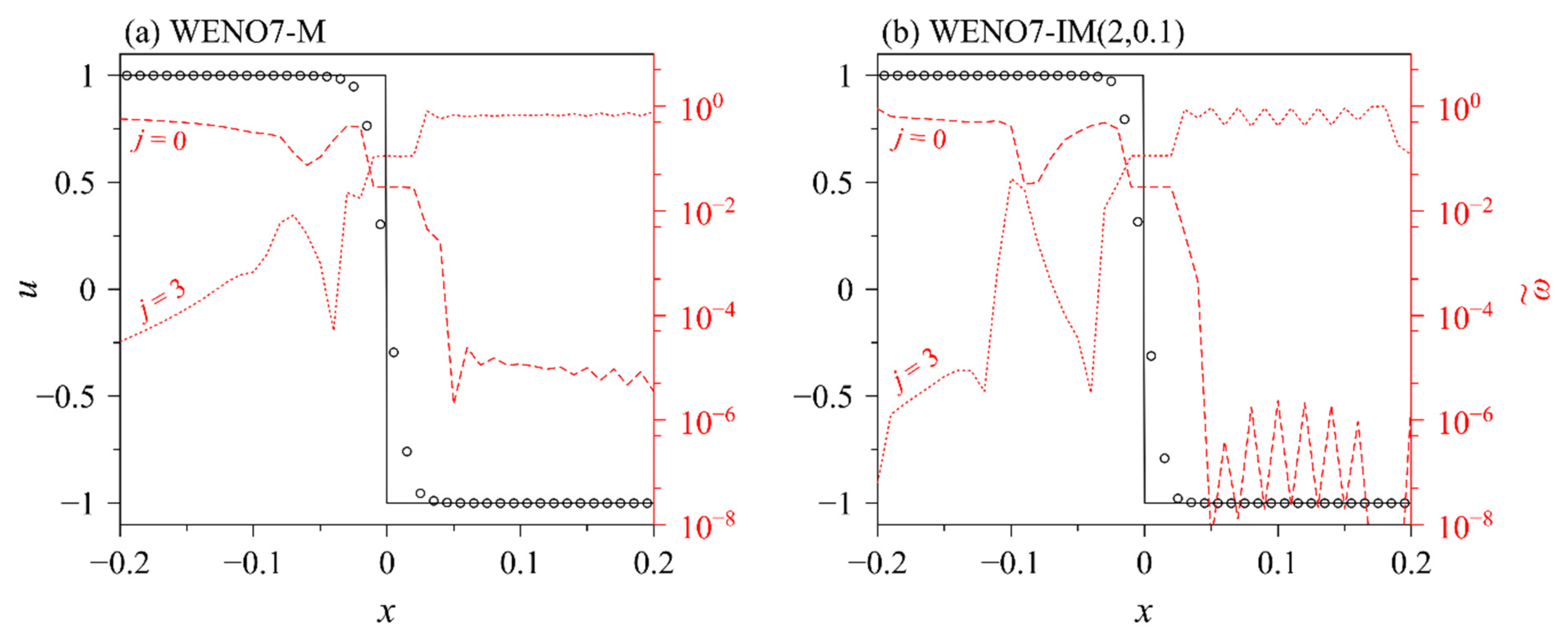
Moving on to seventh-order WENO schemes, the mapped WENO weights of the leftmost (j = 0) and the rightmost (j = 3) stencils WENO-M and WENO-IM(2,0.1) schemes at the end of the first cycle (t = 1 s) are similarly shown in Figure 5. The behaviour of the seventh-order mapped weights is similar to the fifth-order ones across the discontinuity and to its right. To the left of the discontinuity, however, the mapped weights ${\tilde{\omega }}_3$ are relatively larger; for WENO-IM(2,0.1), they are even comparable to ${\tilde{\omega }}_0$ at some locations. This is a crucial difference between the fifth- and seventh-order mapped WENO schemes. It is believed that this difference is due to the small value of $d_0^{\left(4\right)}=\frac{1}{35}$. Referring to the close-up view in Figure 2c, it can be seen that both mapping functions $g_{\mathrm{M}}\left(\omega \right)$ and $g_{\mathrm{IM}}\left(\omega ;2,0.1\right)$ result in particularly severe amplifications to the small weights compared to the identity map (WENO-JS). In fact, the slope of $g_{\mathrm{IM}}\left(\omega ;k,A\right)$ at ω = 0

$${g^{\prime }}_{\mathrm{IM}}\left(0;k,A\right)=1+\frac{1}{A{d}^{k-1}},$$

(23)

is strongly proportional to the inverse of d. Feng et al. [7] have pointed this out and recommended the use of the WENO-M scheme instead of the WENO-IM(2,0.1) scheme for seventh order since ${g^{\prime }}_{\mathrm{M}}\left(0\right)<{g^{\prime }}_{\mathrm{IM}}\left(0;2,0.1\right)$. However, it is clear from Figure 3b and Figure 5 that the WENO-M scheme, while somewhat better than the WENO-IM(2,0.1) scheme, is still inadequate in overcoming the amplification problem for seventh order.

3.2. Proposed Solution

Based on the discussion in the previous section, it appears that limiting the amplification of small weights is important for seventh-order mapped WENO schemes. This idea was pursued in a couple of earlier studies [14,15] by ensuring that the slope of the mapping function vanishes at ω = 0. This actively suppresses near-zero weights. In the present paper, a different, rather simpler approach is suggested to overcome the amplification problem. Consider a general family of rational mapping functions $g_{\mathrm{RM}}$ given as

$$g_{\mathrm{RM}}\left(\omega ;k,m,s\right)=d+\frac{{\left(\omega -d\right)}^{k+1}}{{\left(\omega -d\right)}^k+s{\left[\omega \left(1-\omega \right)\right]}^m},$$

(24)

where k is a positive even integer, m is a positive integer and s is a positive scaling factor. The corresponding mapped WENO scheme will be referred to as WENO-RM(k, m, s). g_RM includes g_IM as a special case for m = 1 and $s=A^{-1}$. Since $\omega$ is a positive real value less than or equal to 1, ω(1 − ω) is a positive quantity with an upper bound of $\raisebox{1ex}{$1$}\!\left/ \!\raisebox{-1ex}{$4$}\right.$. 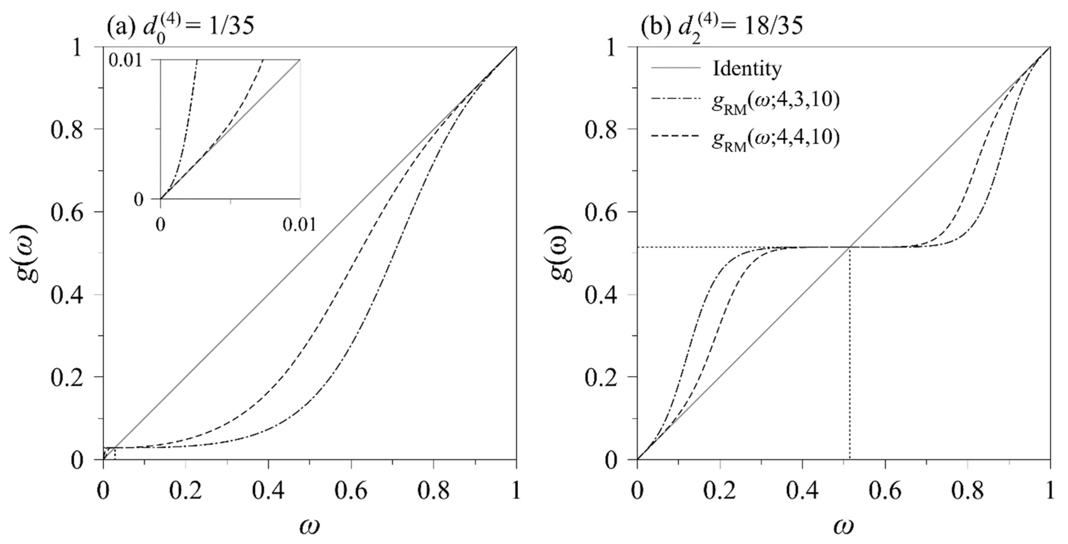Therefore, increasing the value of $m$ allows the term [ω(1 − ω)]^m in the denominator to diminish and, therefore, causes the mapping function to move closer to the identity map g(ω) = ω. In fact, for m > 1, ${g^{\prime }}_{\mathrm{RM}}\left(0;k,m,s\right)=1$, i.e., g_RM functions are able to closely follow the identity map near ω = 0 as shown in the inset plots in Figure 6. This means that, in contrast to previous studies in which small weights were actively suppressed, small weights are preserved with little or no amplification upon mapping with g_RM functions. Therefore, for m > 1, the proposed mapping function g_RM is more suitable for mapped WENO schemes at seventh order and above.

Increasing the values of k and s have the opposite effect of increasing m. Increasing the value of k causes more derivatives of g_RM to vanish at ω = d. Similarly, increasing the value of s would increase the denominator of the rational expression causing the constant term d to dominate. In both cases, the flat portion of the mapping function in the neighbourhood of ω = d is widened, thereby extending the range over which weights get mapped to optimal weights. Feng et al. [7] did not investigate $g_{\mathrm{IM}}\left(\omega ;k,A\right)$ mapping functions beyond k = 2 because increasing k severely amplifies the small weights (see Equation (23)). However, the introduction of parameter m overcomes this restriction and, therefore, a greater range of k values can be explored for mapping functions, which couple better with higher-order WENO methods with m > 1.

Before assessing the performance of any mapping function, it is crucial to verify that it satisfies all the three properties (a)–(c) mentioned earlier. It can be easily verified that g_RM satisfies properties (a) and (c). However, it does not satisfy property (b) unconditionally. g_RM can be non-monotone and determining the exact conditions for monotonicity is not very straightforward. Nevertheless, it can be shown that k ≥ m − 1 is a sufficient condition for monotonicity regardless of the value of s and d (refer to Appendix A). Therefore, the present discussion will be restricted to k ≥ m − 1. It is useful to mention that such restriction is considered reasonable because there are valid values of k that satisfy the monotonicity condition for every value of m.

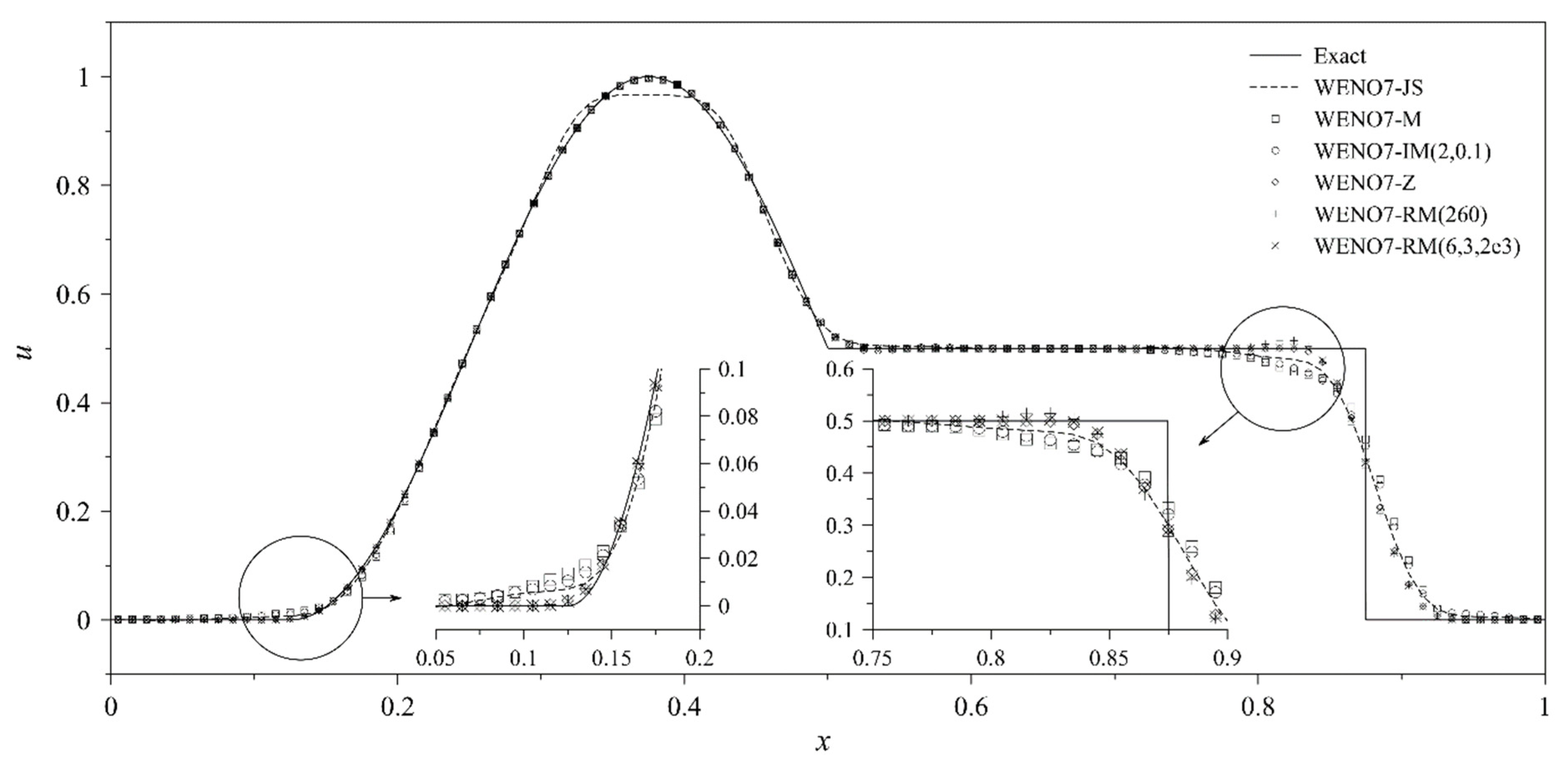
3.3. Parametric Study

A parametric study was conducted to determine good combinations of parameters (k,m,s) using a simple one-dimensional linear advection problem [Equation (20)] with the initial condition given as

$$Case A2 {\overline{u}}_i=\{\begin{array}{cc}\frac{1}{6}\left[G\left(x_i,+\delta \right)+G\left(x_i,-\delta \right)+4G\left(x_i,0\right)\right]& -0.8\le x_i\le -0.6\\ 1& -0.4\le x_i\le -0.2\\ 1-\left|10\left(x_i-0.1\right)\right|& 0\le x_i\le 0.2\\ \frac{1}{6}\left[F\left(x_i,+\delta \right)+F\left(x_i,-\delta \right)+4F\left(x_i,0\right)\right]& 0.4\le x_i\le 0.6\\ 0& \mathrm{otherwise}\end{array},$$

(25)

where $G\left(x,z\right)=\exp \left[-\frac{\log 2}{36{\delta }^2}{\left(x+0.7-z\right)}^2\right]$, $F\left(x,a\right)=\sqrt{\max \left[0,1-100{\left(x-0.5-a\right)}^2\right]}$ and δ = 0.005. From left to right, the initial profile consists of a Gaussian, a square wave, a triangle wave and half-ellipse. This initial condition was first used by Jiang and Shu [5] in their classic paper on WENO schemes. Henceforth, it has become a popular choice for benchmarking numerical methods for hyperbolic problems.

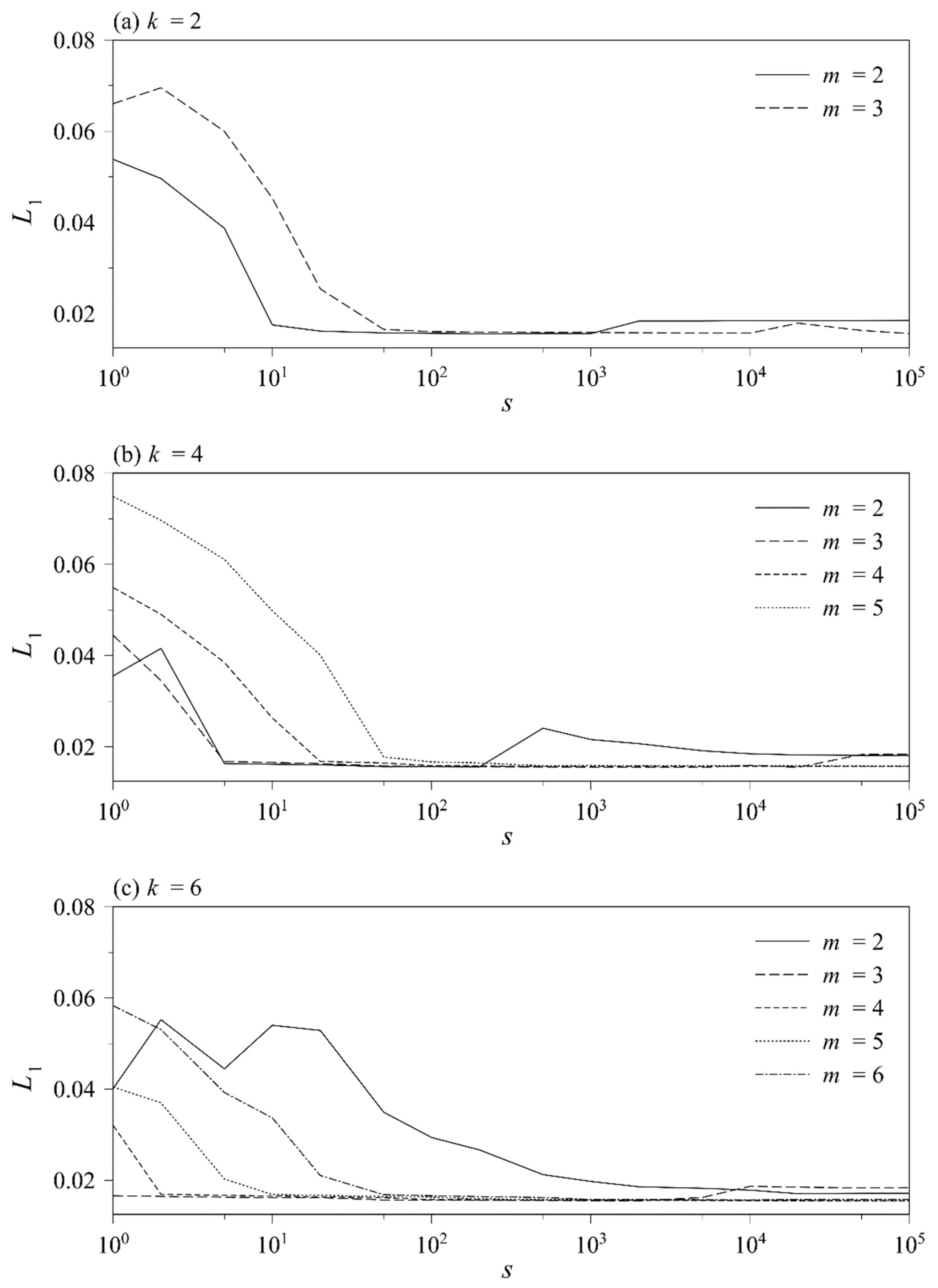
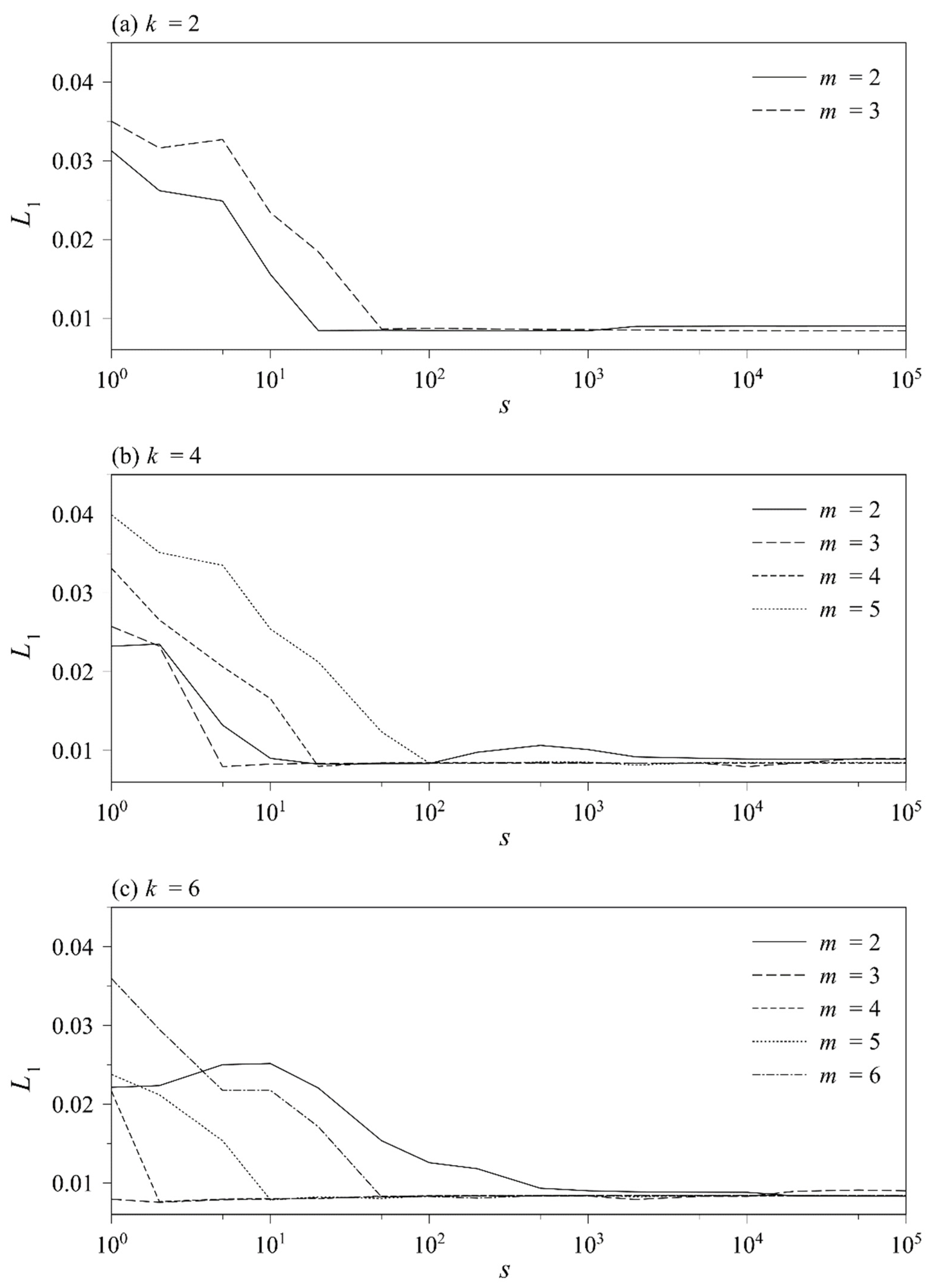
The problem was solved on the domain $x\in \left[-1,1\right]$ at two resolutions, N = 400 and 800 cells. The simulation was run until t = 200 s (100 cycles) using CFL = 0.1. The parameter combinations tested are listed in

Table 1. Parameter combinations used in parametric study.

K	m	s
2	2, 3	1, 2, 5, 10, 20, 50, 100, 200, 500, 1 × 103, 2 × 103, 5 × 103, 1 × 104, 2 × 104, 5 × 104, 1 × 105
4	2, 3, 4, 5
6	2, 3, 4, 5, 6

. The corresponding L₁ error norms are plotted in Figure 7 and Figure 8 for N = 400 and 800 cells, respectively.

A consistent trend can be observed in all cases. For any given combination of k and m, the errors tend to be large for small values of s. Then, the errors reduce with increasing s before increasing slightly at very large values of s. The explanation for this trend is quite intuitive—increasing the value of s extends the range of weights which are mapped to their optimal values. 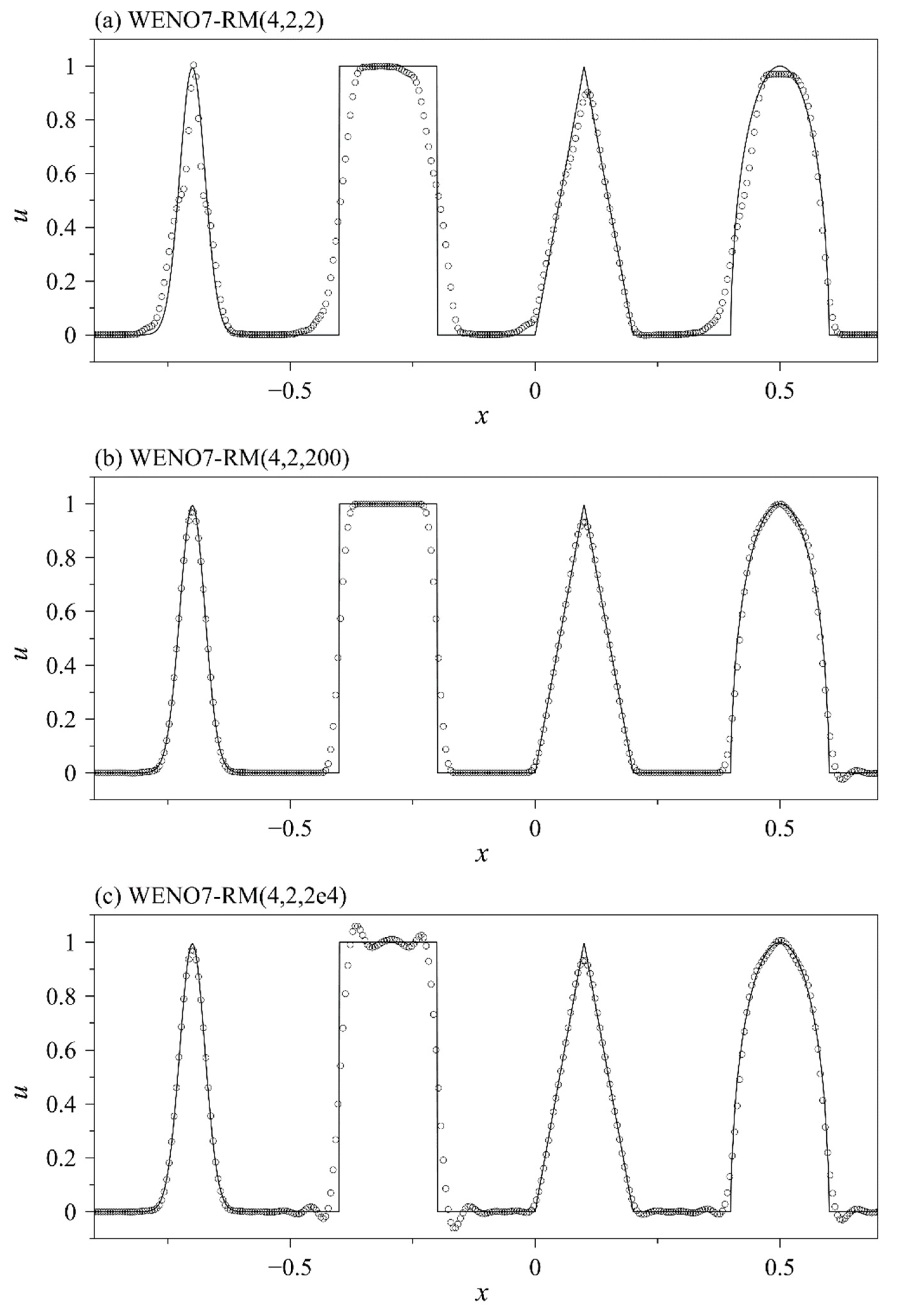Too small a value of s would not map the weights to optimal weights ‘rapidly’ enough resulting in greater numerical diffusion (see discussion in Section 3.1). On the other hand, too large a value would cause the weights to be mapped to optimal weights over-aggressively producing spurious oscillations. This effect is illustrated in Figure 9 for k = 4 and m = 2 at three different values of s. When s = 2, all four profiles suffer distortions. Upon increasing s to 200, the distortions are nearly completely eliminated, and all four profiles are captured well. A small spurious oscillation occurs at the foot of the half-ellipse at x ≈ 0.6. When increased further to s = 2 × 10⁴, prominent spurious oscillations form at the square wave and at the foot of the triangle wave.

Another notable trend is that increasing the value of m almost always results in larger errors at lower values of s. Increasing m causes the mapping function to follow the identity map more closely and decreases the range over which weights are mapped to optimal weights. As such, a large value of s is required to counteract its effect and widen the range before the errors start to reduce. Finally, increasing the value of k tends to have a favourable effect, suggesting that a wide flat region about ω_j = d_j is crucial with the only exception taking place when k is increased from 4 to 6 with m = 2.

Among the various combinations of parameters k, m and s tested, k = 6 and m = 3 consistently results in very low errors over the entire range of s values at both resolutions. However, a suitable value for s appears to be dependent on the problem and resolution. For instance, among the values of s tested, s = 2 × 10³ results in the smallest L₁ error norm when using N = 400 cells. It reduces to s = 2 when using N = 800 cells. However, the choice of the value of s may not be too critical since it is evident from Figure 7 and Figure 8 that the error norms remain small over a wide range of values of s when k = 6 and m = 3.

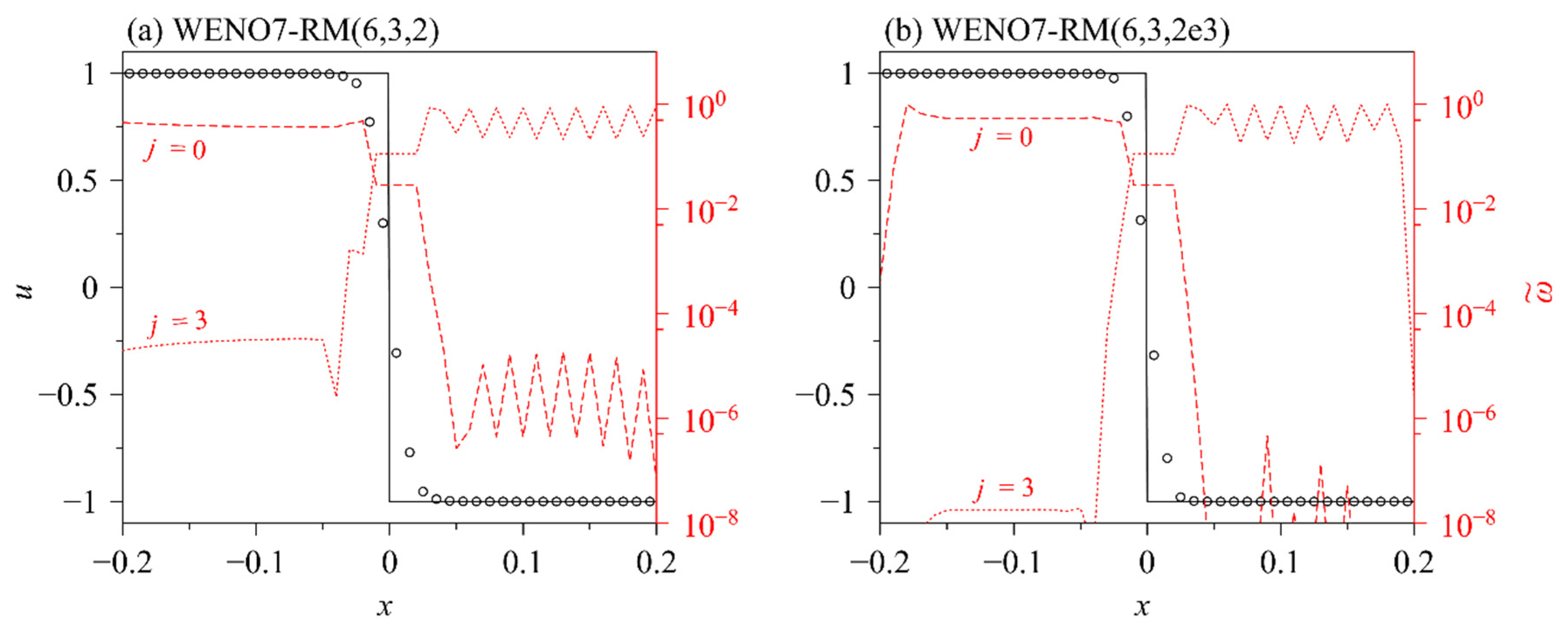
To conclude this section, let us return to linear advection of sharp discontinuities, which motivated the development of this new family of mapping functions. Figure 10a,b show the mapped weights for this problem at t = 1 s (1 cycle) for two different values of s with k = 6 and m = 3. Notice that in both cases, the mapped weights behave in the desired manner without any severe amplification in the flat regions on either side of the smeared discontinuity. It can also be seen that the mapped weights for the non-smooth stencils (j = 0 to the left of the discontinuity and j = 3 to its right) reduce when s is increased. 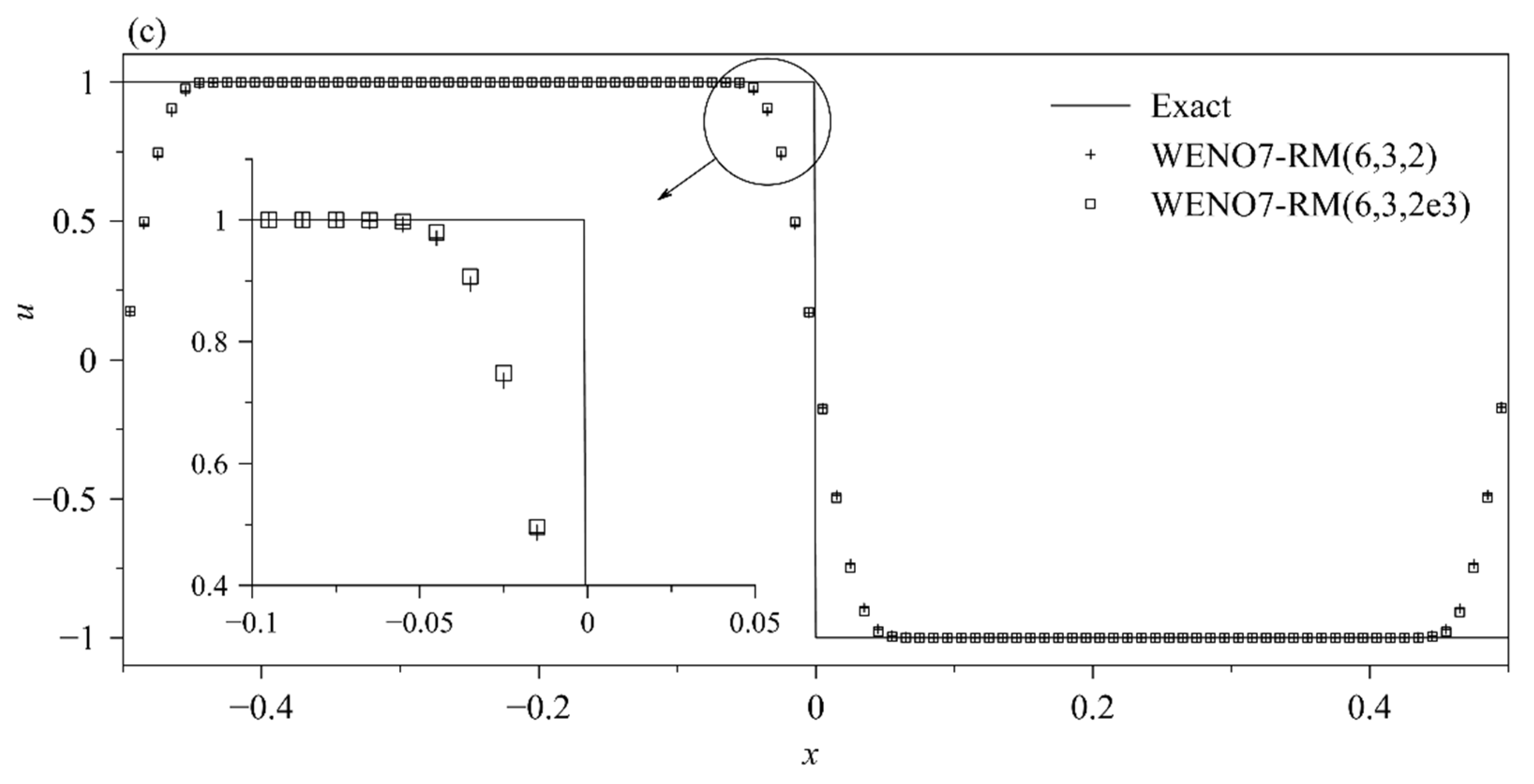This indicates that the discontinuity is captured with less dissipation when using s = 2 × 10³. The final profiles at t = 100 s (100 cycles) using both values of s are shown in Figure 10c. In contrast to the results shown in Figure 3b, the discontinuities are captured well without any distortions for both values of s even at relatively long output times. The close-up view shows that using s = 2 × 10³ indeed results in a slightly sharper discontinuity compared to s = 2. The value of s was chosen to be 2 × 10³ for all the test cases reported in the following section with the exception of the double-Mach reflection Euler problem for which a value of s = 2 was chosen to ensure a stable run.

4. Results

In this section, the proposed schemes are compared with other WENO schemes such as WENO-JS, WENO-M, WENO-IM(2,0.1), WENO-RM(260) [15] and WENO-Z [16]. The value of $ϵ$ was set to 10⁻⁴⁰ for all schemes except for WENO-JS and WENO-RM(260) for which it was set to 10⁻⁶ and 10⁻⁹⁹ [15], respectively. The values of parameters k and m were fixed at 6 and 3, respectively, for all cases. Parameter s was set to 2 × 10³ or 2 corresponding to the WENO-RM(6,3,2 × 10³) or WENO-RM(6,3,2) schemes, respectively. The $\mathrm{CFL}$ number was fixed at 0.1 and 0.5 when solving the advection equation and the Euler equations, respectively.

4.1. Approximate Dispersion Relation

The dispersion relation of a numerical scheme can be used to assess the scheme’s ability to resolve Fourier modes of different wavelengths on a uniform grid. Given a Fourier mode with a wavelength l, its associated wavenumber on a grid with cell spacing $\Delta x$ is $\phi =2\pi \Delta x/l$. Numerical schemes with finite stencils invariably introduce errors in resolving the mode, which results in a modified wavenumber number $\mathsf{\Phi }$. However, it is not possible to derive the exact dispersion relations of non-linear schemes. Instead, Pirozzoli [17] proposed an empirical method to compute approximate dispersion relations of non-linear shock-capturing schemes. The approximate dispersion relations can be used to assess the resolution of the reconstruction scheme in wavenumber space. A uniform N-point mesh supports wavenumbers ${\phi }_k=2\pi k/N$ where $k\in \left[0,N/2\right]$. For each ${\phi }_k$, the one-dimensional linear advection equation Equation (20) is initialized with the sinusoidal mode

$$u_j(0)=\cos \left({\phi }_{k}j\Delta x\right),$$

(26)

for $j\in \left[0,N-1\right]$ and advanced up to a small-time step Δt using the first-order Euler scheme. Next, Fourier transforms are applied to the initial and advanced profiles, and the complex amplitudes ${\widehat{u}}_k\left(0\right)$ and ${\widehat{u}}_k\left(\Delta t\right)$ associated with the kth wavenumber ${\phi }_k$ are used to compute the kth modified wavenumber ${\mathsf{\Phi }}_k$ as:

$${\mathsf{\Phi }}_k=-\frac{\Delta x}{i\Delta t}\log \left(\frac{{\widehat{u}}_k\left(\Delta t\right)}{{\widehat{u}}_k\left(0\right)}\right).$$

(27)

The real and imaginary parts of ${\mathsf{\Phi }}_k$ pertain to the dispersion and diffusion properties of the numerical scheme, respectively. The approximate dispersion relations for the various seventh-order schemes are plotted in Figure 11. The seventh-order upstream central scheme is the linear scheme whereby one simply takes the sub-stencil weights to be the optimal weights, i.e., ω_j = d_j. It represents the optimal resolution that one could achieve from a WENO scheme that relies on the same optimal weights. Hence, it is more meaningful to compare the WENO schemes with the upstream central scheme rather than with spectral methods. The results show that the unmapped WENO-JS scheme has the most deviation from the upstream central scheme and, therefore, the poorest resolution among all schemes. While all mapped WENO schemes and WENO-Z scheme bring about significant improvement over the WENO-JS scheme, the WENO-RM(6,3,2 × 10³) scheme comes the closest to the upstream central scheme in terms of both dispersion and diffusion properties, making it ideal for resolving small-scale flow structures, their convective effects and the induced wave propagation in a high-fidelity simulation of compressible flows where shock waves may also be present. Though the WENO7-IM(2,0.1) scheme follows close behind the WENO7-RM(6,3,2 × 10³) scheme, one must bear in mind that it performs poorly for cases with discontinuities, as demonstrated earlier in Section 3.1.

4.2. Linear Advection

The one-dimensional linear advection problem [Equation (20)] was solved on the periodic domain $x\in \left[-0.5,0.5\right]$ with the smooth initial condition

$$Case A3 {\overline{u}}_i={\sin }^9\left(2\pi x_i\right),$$

(28)

at three different resolutions N = 100, 200 and 400 cells. The L₁ error norms at t = 100 s (100 cycles) are listed in

Table 2. Error norms for linear advection case A3 at t = 100 s (100 cycles).

Schemes	N
	100	200	400
WENO-JS	5.1352 × 10−3	7.1533 × 10−5	6.4335 × 10−6
WENO-M	7.7547 × 10−3	2.6823 × 10−4	7.9258 × 10−6
WENO-IM(2,0.1)	9.7562 × 10−3	8.9693 × 10−4	7.8301 × 10−4
WENO-Z	1.6348 × 10−3	6.0435 × 10−5	6.4376 × 10−6
WENO-RM(260)	1.4095 × 10−3	5.7145 × 10−5	6.4227 × 10−6
WENO-RM(6,3,2 × 103)	1.5083 × 10−3	5.7983 × 10−5	6.4225 × 10−6

.

It can be seen that WENO-JS scheme performs better than both WENO-M and WENO-IM(2,0.1) schemes at all three resolutions. At N = 400 cells, it even surpasses WENO-Z. This is mainly because the relatively large value of $ϵ={10}^{-6}$ overpowers the much smaller values of the smoothness indicators IS_j in the nearly flat regions. As a result, the WENO-JS scheme behaves essentially like the upstream central scheme (ω_j ≈ d_j). Both WENO-M and WENO-IM(2,0.1) schemes perform poorly for this problem, which shows that they are not suitable at seventh order and higher. The proposed scheme WENO-RM(6,3,2 × 10³) delivers a better performance than all other schemes except WENO-RM(260). Nevertheless, its performance improves with increasing resolution, such that at the finest resolution of N = 400 cells, it performs nearly identical to WENO-RM(260).

For the next advection problem, the initial condition

$$Case A4 {\overline{u}}_i=\{\begin{array}{ll}\left[1-\sin \left(4\pi x_i\right)\right]/2\hfill & 1/8<x_i\le 1/2\hfill \\ 1/2\hfill & 1/2<x_i\le 7/8\hfill \\ 0\hfill & \mathrm{otherwise}\hfill \end{array},$$

(29)

was obtained from Ref. [18]. It consists of discontinuities in u at $x=7/8$, $u^{\prime }$ at $x=1/2$ and $u^{″}$ at $x=1/8$. It also possesses a smooth maximum at $x=3/8$. Once again, the problem was solved on the periodic domain $x\in \left[0,1\right]$ at three different resolutions N = 100, 200 and 400 cells. The L₁ error norms at t = 100 s (100 cycles) are listed in

Table 3. Error norms for linear advection case A4 at t = 100 s (100 cycles).

Schemes	N
	100	200	400
WENO-JS	1.6364 × 10−2	7.7120 × 10−3	5.4452 × 10−3
WENO-M	1.5900 × 10−2	1.0101 × 10−2	5.2535 × 10−3
WENO-IM(2,0.1)	1.5687 × 10−2	9.4957 × 10−3	4.1429 × 10−3
WENO-Z	1.0286 × 10−2	5.1822 × 10−3	2.7195 × 10−3
WENO-RM(260)	1.0898 × 10−2	5.1936 × 10−3	2.7181 × 10−3
WENO-RM(6,3,2 × 103)	1.0106 × 10−2	5.0941 × 10−3	2.6748 × 10−3

. The final profiles for N = 100 cells are plotted in Figure 12.

For this case, WENO-RM(6,3,2 × 10³) scheme consistently delivers the best performance at all three resolutions. Once again, both mapped WENO schemes WENO-M and WENO-IM(2,0.1) deliver poor performances especially near the discontinuity in u at x = 7/8 and the discontinuity in $u^{″}$ at x = 1/8, as shown in Figure 12. The WENO-JS scheme is unable to capture the smooth maximum at the coarse resolution of N = 100 cells, but it is able to do so at the finer resolutions. WENO-Z and WENO-RM(260) schemes deliver similar performances except at the coarsest resolution of N = 100 cell, whereby the WENO-RM(260) scheme results in a small overshoot on the left side of the discontinuity at x = 7/8. This is quite surprising since WENO-RM(260) is a mapped WENO scheme that actively suppresses small weights. The overshoot does not occur at the finer resolutions though.

4.3. Euler Equations

The system of one-dimensional Euler equations for an ideal gas is given as

$${\partial }_t\left(\begin{array}{c}\rho \\ \rho u\\ \rho e\end{array}\right)+{\partial }_x\left(\begin{array}{c}\rho u\\ \rho u^2+p\\ \rho hu\end{array}\right)=\mathbf{0},$$

(30)

where ρ, u and p refer to the gas density, velocity and pressure, respectively. The specific total energy is given by $e=p/\left(\gamma -1\right)\rho +u^2/2$ and the specific total enthalpy by $h=e+p/\rho$. γ is the ratio of specific heats with a value of 1.4. The system was solved using a hybrid method coupling a MUSCL-type flux approach and HLL-based characteristic flux approach using a shock sensor [19].

The first case Is a shock tube problem proposed by Lax [20]. The initial condition

$$Case E1 \left(\rho ,u,p\right)=\{\begin{array}{cc}\left(0.445,0.698,3.528\right)& x<0\\ \left(0.500,0.000,0.571\right)& x\ge 0\end{array},$$

(31)

consists of two constant states separated by a discontinuity at x = 0. The problem was solved on the domain $x\in \left[-0.5,0.5\right]$ until t = 0.13 s. The final density profiles are shown in Figure 13.

For this case, all the improved WENO schemes capture a sharper contact discontinuity at x = 0.2 and a sharper shock at x = 0.32 compared to the WENO-JS scheme. WENO-RM(6,3,2×10³) scheme captures the sharpest discontinuities among all schemes. All the schemes, including the WENO-JS scheme, result in spurious oscillations to the right of the contact discontinuity to some extent, but WENO-Z is the only scheme to cause a large overshoot and a small undershoot to left and right of the shock, respectively. It must be mentioned that the WENO-RM(260) scheme results in the smallest spurious oscillation among the improved WENO schemes.

The next two test cases are shock-entropy wave interaction problems proposed by Shu and Osher [21] and Titarev and Toro [22]. The corresponding initial conditions are given in Equations (32) and (33), respectively.

$$Case E2 \left(\rho ,u,p\right)=\{\begin{array}{cc}\left(3.857143,2.629369,10.33333\right)& x<-4\\ \left(1+0.2\sin \left(5x\right),0,1\right)& x\ge -4\end{array}$$

(32)

$$Case E3 {\left(\rho ,u,p\right)}_0=\{\begin{array}{cc}\left(1.515695,0.523346,1.80500\right)& x<-4.5\\ \left(1+0.1\sin \left(20x\right),0,1\right)& x\ge -4.5\end{array}$$

(33)

The interaction of the shock with the entropy wave results in short-wavelength structures whose amplitudes are a good measure of the numerical viscosity of the numerical scheme. These structures are representative of the large-scale eddies encountered, for instance, in the wake of an airfoil undergoing flow separation. Case E3 is a more severe version of case E2 as it results in structures of much shorter-wavelength structures compared to the latter case, potentially more representative of the finer-scale turbulent structures and their fluctuations in the flow. Case E2 was solved on the domain $x\in \left[-5,5\right]$ discretized into N = 200 uniform cells until t = 1.8 s. Case E3 was solved on the same domain discretized into N = 1000 cells until t = 5 s. The reference solutions for both cases were obtained on a fine grid with ten times the resolution. The final density profiles are shown in Figure 14 and Figure 15.

The performance trends are similar for both cases. Once again, WENO-JS results in the smallest amplitudes for the short-wavelength structures among all schemes. The best performance is delivered by the WENO-RM(6,3,2×10³) scheme, which is closely followed by WENO-IM(2,0.1) and WENO-RM(260). Surprisingly, WENO-Z does not perform as well as in the advection cases; its performance is only slightly better than that of WENO-M.

For the last case, we consider the two-dimensional double Mach reflection (DMR) problem proposed by Woodward and Colella [23], in which a strong Mach 10 shock wave impinges obliquely onto a ramp and undergoes a complex reflection producing intricate flow features. The WENO schemes were extended to higher dimensions by applying the one-dimensional schemes along the local face-normal direction. This approach is significantly cheaper and more robust compared to a fully multi-dimensional formulation. The DMR problem was computed using one of the alternative setups suggested by U S Vevek et al. [24], whereby the shock wave makes an angle of $\theta ={\tan }^{-1}\left(\frac{7}{4}\right)\approx 60.26°$ with the ramp. This enables exact tracking of the shock wave along the top boundary on a uniform structured mesh. The problem was computed on the domain $x\times y\in \left[0,4\right]\times \left[0,1\right]$ discretized into the uniform cells of width $\Delta x=\Delta y=\raisebox{1ex}{$1$}\!\left/ \!\raisebox{-1ex}{$240$}\right.$. The ramp extends along the bottom boundary from x = 1 to the right. Reflective boundary conditions are applied along the ramp and Neumann boundary conditions are applied along the remainder of the bottom boundary from x = 0. The exact pre- and post-shock conditions

$$Case E4 \begin{array}{l}{\left(\rho ,u,v,p\right)}_{pre}=\left(1.4,0,0,1\right),\\ {\left(\rho ,u,v,p\right)}_{post}=\left(8,-8.25\cos \theta ,8.25\theta ,116.5\right),\end{array}$$

(34)

were prescribed at the right and left boundaries, respectively. The terms u and v denote the horizontal and vertical velocity components, respectively. The shock wave was initialized to intersect the bottom boundary at x = 0.1 and the simulation was computed until t = 0.27 s with a re-initialization at an intermediate time t = 0.08 s to prevent undesirable numerical artefacts. The final results are plotted in Figure 16, using 41 equally spaced density contours in the range $\rho \in \left[1.4,21.4\right]$.

The WENO-IM(2,0.1), WENO-Z and WENO-RM(6,3,2 × 10³) schemes became unstable for this problem within the first few time steps. These schemes are most likely too aggressive near the shock wave in that they do not introduce sufficient numerical diffusion. It must be recalled from the previous section that both s = 2 and s = 2 × 10³ led to distortion-free results for the linear advection of the discontinuities problem (see Figure 10), and the latter was chosen on the grounds that it produced a slightly sharper discontinuity. However, since this leads to an unstable scheme for the DMR problem, the value of parameter s was chosen to be 2 for this problem alone for a stable computation. It can be seen from Figure 16 that there are not many notable differences in the results computed using the different schemes except some minor differences along the slip line. The lack of roll-ups along the slip line may be surprising to some, but it has been demonstrated in [19] that the choice of reconstructed variables and flux scheme has an effect on the extent of the details captured along the slip lines and that the usual notion of more roll-ups being indicative of a better, less diffusive scheme need not necessarily hold true in all cases.

The results obtained using the WENO-RM(6,3,2) scheme for the other Euler cases were similar to those obtained using the WENO-RM(260) scheme, but the former scheme was computationally more efficient. For instance, for the DMR problem, the WENO-RM(6,3,2) scheme was 16% slower than the unmapped WENO-JS scheme, whereas the WENO-RM(260) scheme was 83% slower.

5. Conclusions

This paper was motivated by the poor performance of the mapped WENO schemes WENO-M and WENO-IM(2,0.1) in capturing discontinuities accurately over long output times. While WENO-M performed poorly at both fifth and seventh orders, WENO-IM(2,0.1) performed poorly only at seventh order. By observing the mapped stencil weights ${\tilde{\omega }}_j$ near the discontinuities, it was argued that the superior performance of the fifth-order WENO-IM(2,0.1) scheme was attributed to the wider flat portion of $g_{\mathrm{IM}}\left(\omega ;2,0.1\right)$ in the neighbourhood ω_j = d_j. The fifth-order WENO-M scheme, on the other hand, had a narrower flat portion at about ω_j = d_j, which resulted in increased numerical diffusion since it did not bring the weights close to their optimal values as quickly.

At seventh order, both WENO-M and WENO-IM(2,0.1) schemes performed poorly due to severe amplification of small weights. While such amplification also occurred at fifth order, it was not as severe due to the relatively larger numerical values of d_j at fifth order compared to the seventh order. A simple solution was suggested in the form of a more general family of mapping functions $g_{\mathrm{RM}}\left(\omega ;k,m,s\right)$ which includes $g_{\mathrm{IM}}\left(\omega ;k,A\right)$ as a special case. For m > 1, these mapping functions have a unit slope at ω = 0 regardless of the values of d_j. This prevents the over-amplification of small weights, making it particularly suitable for seventh order and above. The values of parameters k, m and s were determined to be 6, 3 and 2 × 10³, respectively, based on a parametric study. The resulting mapped WENO scheme is referred to as WENO-RM(6,3,2 × 10³).

It was shown through a number of one-dimensional linear advection problems that the WENO-RM(6,3,2 × 10³) scheme outperformed both the WENO-M and WENO-IM(2,0.1) schemes. It was able to deliver similar or even superior performances compared to other popular WENO schemes such as WENO-RM(260) and WENO-Z. It was also shown that the proposed scheme performed the best among all the schemes tested, for a number of one-dimensional inviscid gas flow problems. It was able to capture the sharpest discontinuities in the shock tube problem and greatest amplitudes for the short wavelength structured in shock-entropy wave interaction problems. It should also be quickly remarked that these conclusions are equally applicable to the finite difference method as the finite difference and finite volume methods are equivalent in one dimension. The WENO-RM(6,3,2) scheme was used for the two-dimensional DMR problem alone because the WENO-RM(6,3,2 × 10³) scheme was unstable for this problem. The key lesson from the DMR problem is that the value of parameter s is case dependent. In fact, even for a single case, it would be better to allow parameter s to vary locally based on the solution.

The insights gleaned from this study were the basis for the successful development of the adaptive mapped WENO scheme [25]. The adaptive scheme relies on the g_RM family of mapping functions introduced in the present paper but, instead of using a constant value for s, it uses an adaptive value calculated based on the local smoothness of the solution.