Framework for Estimating Performance and Associated Uncertainty for Modified Aircraft Configurations

Abstract

Flight testing has been the historical standard for determining aircraft airworthiness. However, increases in the cost of flight testing and the accuracy of inexpensive CFD encourage the adoption of certification by analysis to reduce or replace flight testing. A framework is introduced to predict the performance in the special case of a modification to an existing, previously certified aircraft. This framework uses a combination of existing flight tests or high fidelity data of the original aircraft as well as lower fidelity data from CFD or wind tunnel testing of the original and modified configurations to create 6-DOF flight dynamics models. Two methods are presented which generate an updated flight dynamics model and estimate the model form uncertainty for the modified aircraft configuration using knowledge of the original aircraft. This updated dynamics model and uncertainty estimate are then used to conduct non-deterministic simulations with wind turbulence included. The framework is applied to an example aircraft system to demonstrate the ability to predict the performance and associated model from the uncertainty of modified aircraft configurations.

1. Introduction

The aircraft airworthiness certification process has traditionally relied on flight testing to determine whether the system meets the minimum standards of airworthiness, safety of flight, and risk [1]. Organizations tasked with airworthiness certification, such as the Federal Aviation Administration (FAA) and Naval Air Systems Command (NAVAIR), can consider modifications, such as an added radome, to a previously certified aircraft as an entirely separate aircraft for the purposes of certification [1,2,3]. Because these modifications are about a single reference aircraft, performing time-consuming and expensive flight tests may not be justified for some modifications.

There is currently interest in certification by analysis, or the use of analysis and simulation to supplement or replace flight testing in the certification process, in the aviation community-notably by the AIAA Certification by Analysis (CbA) Community of Interest (CoI), which released a set of recommended practices in 2021 [4]. In particular, there is a desire to use analysis and simulation to model modifications to a previously certified aircraft and associated uncertainties [5]. These modified configurations must still be accurately modeled and simulated with limited or no flight test data in order to meet the standards of airworthiness with the same level of confidence [5]. Performing uncertainty quantification is considered an essential part of the certification by analysis process and ensures that performance estimates take into consideration modeling and simulation errors and uncertainties [4]. Certification by analysis is already commonly done in the nuclear industry, due to the high risks and costs associated with testing [6]. This paper proposes a framework using uncertainty analysis and non-deterministic simulations to estimate the flight performance of modified aircraft configurations without requiring flight test data of the modified configuration. In the future and with additional development, this estimated performance could then be used to reject unsuitable configurations or otherwise inform the flight test process.

Uncertainty quantification is of growing importance in the field of modeling and simulation, especially for aerospace applications [7,8]. There are various types of uncertainty, including input uncertainty, numerical uncertainty, and model form uncertainty [9]. The present research focuses on model form uncertainty, which originates due to the structure of the selected model (for example, by neglecting higher order or non-linear terms) [7,8]. Uncertainty, including model form uncertainty, can be placed into two categories. The first, epistemic uncertainty is due to a lack of knowledge and is represented by the range of possible values, without knowledge of the distribution [9,10,11]. Aleatory uncertainty is due to inherent randomness and is usually characterized probabilistically [9,10,11]. Quantifying and accounting for model form uncertainty is especially important when considering conditions where experimental data are limited or non-existent [6,9,10].

Uncertainty analysis can be an important aspect throughout all phases of aircraft simulation and modeling, including design, testing, and evaluation. Uncertainty quantification and analysis is frequently performed on Computational Fluid Dynamics (CFD) results at many stages of the code development and use [12]. Previously, uncertain terms have been used to perform deterministic simulations where the aerodynamic parameters are updated following the simulation, but are not varied during the simulation [13]. Uncertain wind gusts have been used in non-deterministic aerodynamics simulations with known aerodynamic parameters, especially looking at the effects on aircraft loading [14]. Simulations using aerodynamic uncertainty have also been used to aid in the design process by allowing for improvements to technology to be incorporated into the process and ensuring that new designs are capable of meeting the same certification standards [15]. Non-deterministic simulations have been used as sub-components of more complex aircraft simulations, allowing for analysis of uncertainty within a given component, such as the fuel systems [16].

Full non-deterministic aircraft flight dynamics simulations have been previously used to evaluate the performance of an aircraft in a variety of conditions and when the aircraft dynamics are not known exactly [17,18]. Prior work included using a baseline model of the aircraft dynamics, created using flight test data, which was then tuned using additional flight test data [17]. Probability Bounds Analysis (PBA) was used to calculate uncertainty bounds for the aircraft dynamics and non-deterministic simulations were then conducted [17]. PBA allows for the creation of uncertainty bounds for model form uncertainty by a comparison of the simulation and experimental data [18,19]. The non-deterministic simulations allow for estimates of aircraft performance, given uncertainties in the aircraft dynamics, for a range of environments, allowing for the probability of loss of control prediction [17]. The results can also be extended to other quantities of interest during the airworthiness certification process, such as maximum winds allowed, climb rate, and landing distance.

Modifications to existing aircraft configurations can have a dearth of data compared to the existing aircraft, including data from wind tunnel tests, flight tests, and Computational Fluid Dynamics (CFD), depending on the development of the proposed modification. To provide additional resources for the flight certification process, non-deterministic simulations of modified aircraft configurations are proposed. Since there might not always be flight test data available for model tuning, uncertainty quantification, and non-deterministic simulations for these modified configurations, the proposed process uses knowledge of the unmodified, nominal configuration to assist in the simulation of the modified configuration. Two methods are proposed to estimate the modified aircraft dynamics and the uncertainties of the modified aircraft dynamics, using aspects of the nominal system, which can then be used to perform non-deterministic simulations. This framework is designed independently of the source or quality of the data, as well as the model form or accuracy (for example, a linear model created using CFD data). Because this framework includes an estimate of the uncertainty for the modified configuration alongside a prediction of performance, it can be considered an early step towards certification by analysis. The framework can also be used prior to flight testing to provide an estimate of expected performance.

The proposed approach relies on a set of models. The models and their interaction will be defined in detail in subsequent sections. For the sake of clarity, we summarize the models here:

• Baseline model: this is a computational model of the original, certified aircraft.
• Tuned model (also known as flight test model or observed model): this is a model obtained from the observation of the baseline model.
• Updated model: this is a model of the modified aircraft configuration, generated using one of the two proposed methods to account for changes due to the modification.

First, the approach for calculating the initial models, as well as the uncertainty for the nominal system, is described. Next, the two methods of estimating the model and uncertainty for the modified configurations using knowledge of the uncertainty of the nominal system are introduced. These methods are then validated using simulated aircraft data, using the method of manufactured universes framework, which takes advantage of simulated data when typical validation data are unavailable [20]. The paper concludes with observations of the proposed framework and areas of future research.

2. Analysis of Nominal Configuration

One of the goals of this research is to estimate the flight performance and associated uncertainty of a modified aircraft configuration, without requiring flight test data for the modified configuration. For the purposes of this research, a modified configuration is a configuration that differs from the nominal configuration by one or more modifications, such as payload pods, increase in mass, or change in wing characteristics. For most aircraft with multiple configurations, there is often a configuration which is considered “nominal” and is the basis for any modifications. Although the nominal configuration will likely have flight test data or other higher fidelity data, the modified configurations may only have limited data available, typically from CFD or wind tunnel tests.

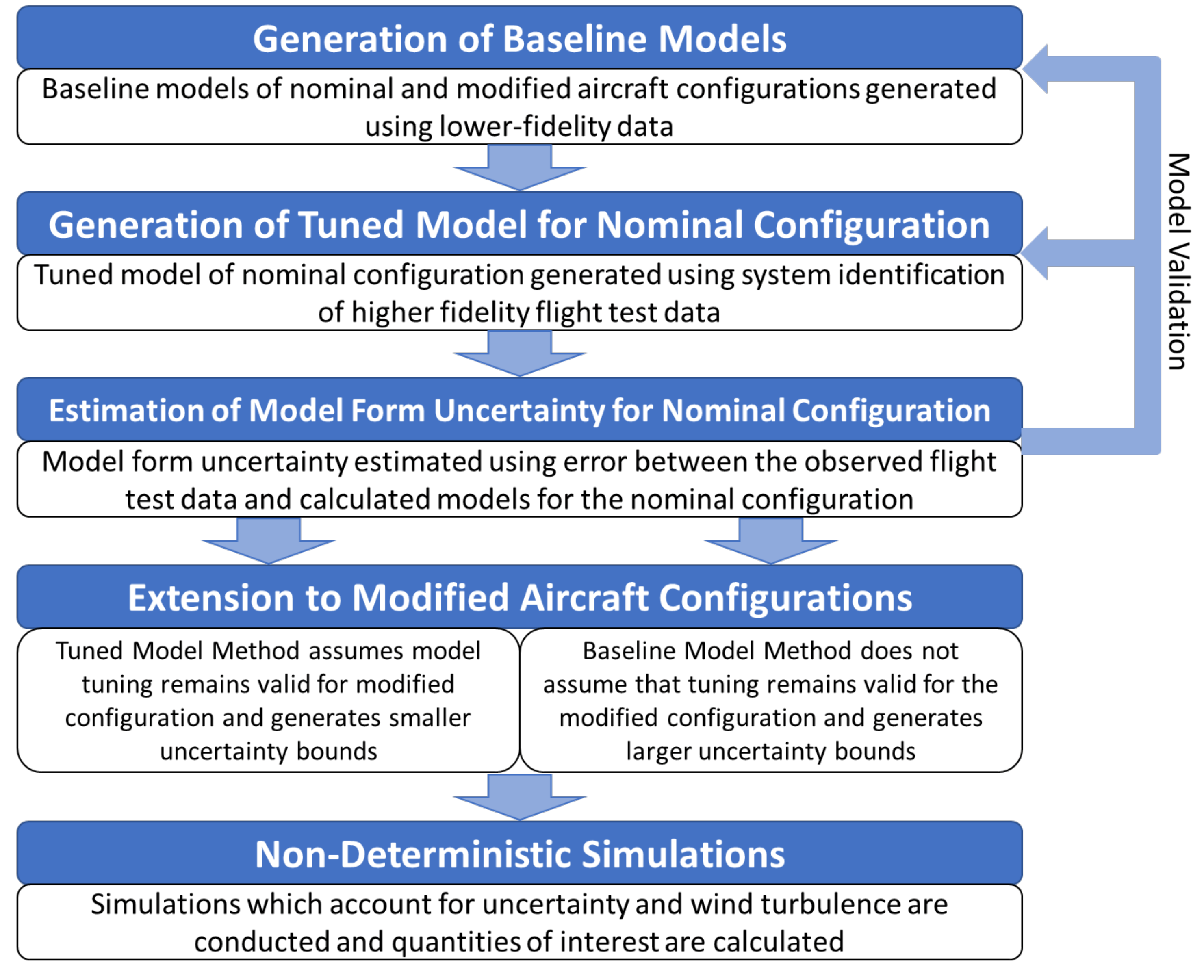
2.1. Generation of Baseline Models

The first model that is generated for the nominal configuration is the baseline model, which serves as a common denominator for corrections and modifications. This model should ideally be developed using a data collection method which is available for the nominal configuration as well as any modified configurations. For instance, CFD data is available for the nominal configuration and many modified configurations for the AeroStar aircraft used as a research testbed by NAVAIR, but flight test data are not available for all configurations. Because the baseline model will often be generated using CFD data, it may often be referred to as a computational model. However, this does not mean that a model made from the preliminary or conceptual design of the aircraft will be sufficient - it is assumed that the aircraft is modeled with sufficient accuracy. Such models are frequently used throughout the design and development process. For the nominal configuration, an example aerodynamic coefficient for this model is indicated by $C_{*}^{base}$. Similarly, a baseline model for the modified configuration is also created, $C_{*}^{base}+\delta C_{*}^{base}$.

2.2. Generation of Tuned Model

The next model generated for the nominal configuration is the tuned model, which utilizes the most accurate data available, generally flight test data. This model may also be known as a flight test model or observed model and are often used for the development and testing of control algorithms before incorporating them into flight vehicles. While these data are more accurate, they may not exist for all configurations, so a tuned model can only be created for the nominal configuration. This tuned model will generally have the same model form (linear or non-linear) as the baseline model, but it is not required to. The difference between the tuned model of the nominal configuration and the baseline model of the same configuration is represented by $\Delta C_{*}^{tun}$. An improved model of the nominal configuration is then represented by $C_{*}^{nom}=C_{*}^{base}+\Delta C_{*}^{tun}$.

Often, this model will be generated using parameter identification of flight test data but could include higher fidelity CFD or wind tunnel data. Common parameter estimation techniques used to generate the model include equation error method, output error method, and filter error method, which are described in Ref. [21].

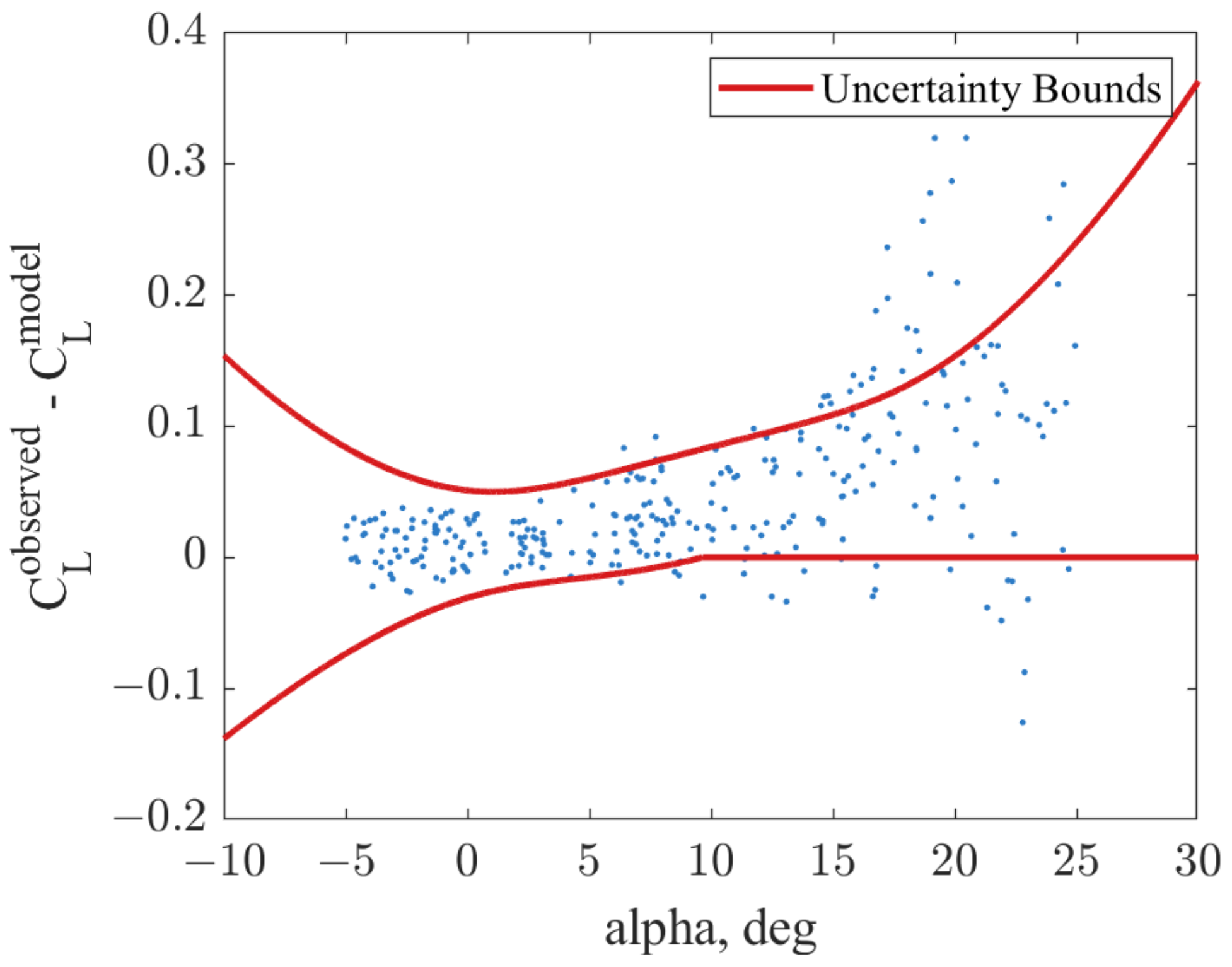
2.3. Estimation of Model Form Uncertainty

The uncertainty of the greatest interest for this research is model form uncertainty, or uncertainty due to the difference between the model and the true system. However, the limited availability, poor quality, or inherent noise of these data sources can contribute to additional uncertainty associated with the model.

To calculate this uncertainty, the model is evaluated at each time step of the flight test data and is then compared to the values from the original data. This generates a series of time-independent errors for each timestep, as shown in Figure 1 with blue dots for each timestep. Uncertainty bounds are estimated using 95% confidence intervals on the mean error between the higher fidelity data and the baseline or tuned model for each equation of motion as (1) [17,22]:

$$\widehat{y}\left(x_o\right)-t_{\alpha /2,n-p}\sqrt{{\widehat{\sigma }}^2{x}_0^{\prime }{\left(X^{\prime }X\right)}^{-1}{x}_o}\le {\mu }_{y|x0}\le \widehat{y}\left(x_o\right)+t_{\alpha /2,n-p}\sqrt{{\widehat{\sigma }}^2{x}_0^{\prime }{\left(X^{\prime }X\right)}^{-1}{x}_o}$$

(1)

where $\widehat{y}\left(x_0\right)$ is the model response about the aircraft state $x_0$, $t_{\alpha /2,n-p}$ is the Student’s t-distribution for $100(1-\alpha$) confidence interval with $n-p$ degrees of freedom (where n is the number of samples and p is the degree of the polynomial), ${\widehat{\sigma }}^2$ is the sample standard deviation, ${\mu }_{y|x0}$ is the mean error of the model response at the aircraft state, and X is the matrix of observed data. These bounds are shown in Figure 1 as red lines; note that the bounds used in non-deterministic simulations are modified from those calculated to always include zero error to prevent changes to the model form or tuning. Some of the time-independent errors, shown as blue dots, are outside of the uncertainty bounds; this is expected due to the 95% confidence interval used to calculate the bounds as well as any slicing needed to represent multi-dimensional bounds in a two-dimensional figure. Because the bounds are dependent upon the state of the aircraft, they can be correlated with specific states, allowing for smaller bounds where there are more data and increased bounds where data are sparse, as in Ref. [17]. Because the bounds grow exponentially as they move away from the available data, prediction for aircraft states far from observed values can lead to high uncertainty, as expected.

This uncertainty can be calculated about both the baseline and tuned models, creating two different uncertainty bounds, as shown in Figure 2 and Figure 3. When adding the uncertainty to our model of the nominal configuration, $C_{*}^{nom}$, two equations emerge, dependent on whether the tuning correction is used:

$$C_{*}^{nom}=C_{*}^{base}\pm \Delta C_{*}^{UQ}{|}_{base}$$

(2)

and

$$C_{*}^{nom}=C_{*}^{base}+\Delta C_{*}^{tun}\pm \Delta C_{*}^{UQ}{|}_{tun}$$

(3)

2.4. Extension to Modified Aircraft Configurations

In order to perform non-deterministic simulations of modified aircraft configurations, an estimate of the model form uncertainty must first be obtained. Section 3 discusses the two methods to estimate this uncertainty based on the models of the nominal and modified configurations and flight test data for the nominal configuration.

2.5. Non-Deterministic Simulation

Non-deterministic simulations are conducted using the baseline and tuned models while accounting for changes due to modifications as well as uncertainty. Using the previously calculated uncertainty bounds, uncertainty in the states is added at each time step, dependent on the current state and control inputs. The simulation also includes a turbulent wind component, which adds additional realistic uncertainty to the simulation and better matches the simulated flight test data. To fully capture the uncertainty of the aircraft design, multiple independent simulation runs are combined to create a range of expected performance. Bounds of the estimated flight performance are calculated by taking 95% of the combined simulation data. Convergence analysis of the simulation results is performed to demonstrate the number of simulation runs to achieve suitable convergence.

3. Analysis of Modified Configurations

A flight dynamics model for a modified configuration can be obtained from CFD or wind tunnel test data, but accounting for the difference between the model and flight test data for the nominal configuration, known as the tuning correction, allows for a better estimate of the true flight performance. The model form uncertainty of the modified configuration cannot be calculated without flight test data, but this uncertainty is valuable as a method to bound the predicted performance and capture the effects that cannot be easily obtained by ground-based testing. Since there is no direct way to calculate the model form uncertainty for the modified configuration, it must be estimated.

This framework addresses the desire to accurately predict and bound the performance of modified aircraft configurations by utilizing knowledge of the nominal, unmodified configuration. Figure 4 illustrates the major stages of the framework. First, baseline models of the nominal configuration and any modified configurations are generated using lower fidelity data, such as CFD. Second, a tuned model of the nominal configuration is generated using system identification of available flight test data. Using these models and the flight test data, model form uncertainty is then estimated. Before proceeding, the models and uncertainty are validated to confirm that the models are adequate for their intended use [23]. Next, one of two methods described in Section 3.1 and Section 3.2 are used to extend the aerodynamic model and uncertainty estimation to the modified configurations. Finally, non-deterministic flight dynamics simulations which account for uncertainty as well as wind turbulence are conducted in order to predict the performance and associated uncertainty bounds of the modified configurations.

The first step in modeling a modified configuration is modeling the nominal, unmodified configuration, described in Section 2. The framework will be illustrated using a single model term but can be applied to all terms in the aircraft dynamics model. The nominal configuration of this aircraft can be described using a combination of the baseline model $C_{*}^{base}$, model tuning $\Delta C_{*}^{tun}$, and uncertainty $\Delta C_{*}^{UQ}$. Since we can calculate the model form error, which leads to the model form uncertainty, of the nominal configuration about both the baseline and tuned model, there are two related models, described above in Equations (2) and (3).

Equation (2) describes the case where the uncertainty is calculated about the baseline model, $C_{*}^{UQ}{|}_{base}$, whereas Equation (3) describes the case where the uncertainty is calculated about the tuned model, $C_{*}^{UQ}{|}_{tun}$. For the nominal configuration, which has both lower fidelity and higher fidelity data and is, therefore, able to be tuned, Equation (3) is more accurate and should always be used, but both equations are given to aid in developing the two methods for modeling for the modified configuration.

When we describe a modified aircraft configuration using the same nomenclature, additional terms appear due to the change in configuration. After including additional model tuning to match flight test data and uncertainty quantification, the final model for the modified configuration can be written in two different ways, corresponding to Equations (2) and (3):

$$C_{*}^{mod}=C_{*}^{base}\pm \Delta C_{*}^{UQ}{{|}_{base}+\delta C_{*}^{base}\pm \delta C_{*}^{UQ}|}_{base}$$

(4)

$$C_{*}^{mod}=C_{*}^{base}+\Delta C_{*}^{tun}\pm \Delta C_{*}^{UQ}{{|}_{tun}+\delta C_{*}^{base}+\delta C_{*}^{tun}\pm \delta C_{*}^{UQ}|}_{tun}$$

(5)

where $\delta$ indicates the change due to modification in the configuration, $\delta C_{*}^{base}$ is the change to the baseline model due to the modified configuration, $\delta C_{*}^{tun}$ is the additional correction due to model tuning (if available) for the modified configuration, and $\delta C_{*}^{UQ}$ is the additional uncertainty for the modified configuration. Although $\delta C_{*}^{base}$ can be obtained by comparing lower fidelity data of the nominal and modified configurations, such as wind tunnel or CFD data, $\delta C_{*}^{tun}$ and $\delta C_{*}^{UQ}$ cannot be calculated without higher fidelity data for the modified configuration, such as flight test data, which are often unavailable.

Using the prior knowledge of the nominal configuration, two methods are proposed to estimate the uncertainty of the modified configuration [24]. The methods differ in the approximation of $\delta C_{*}^{tun}$ and $\delta C_{*}^{UQ}$ and do not require parameter tuning and uncertainty quantification for the modified configuration. The methods are intended for small and large modifications, respectively, although the applicability of each method will be explored in future work.

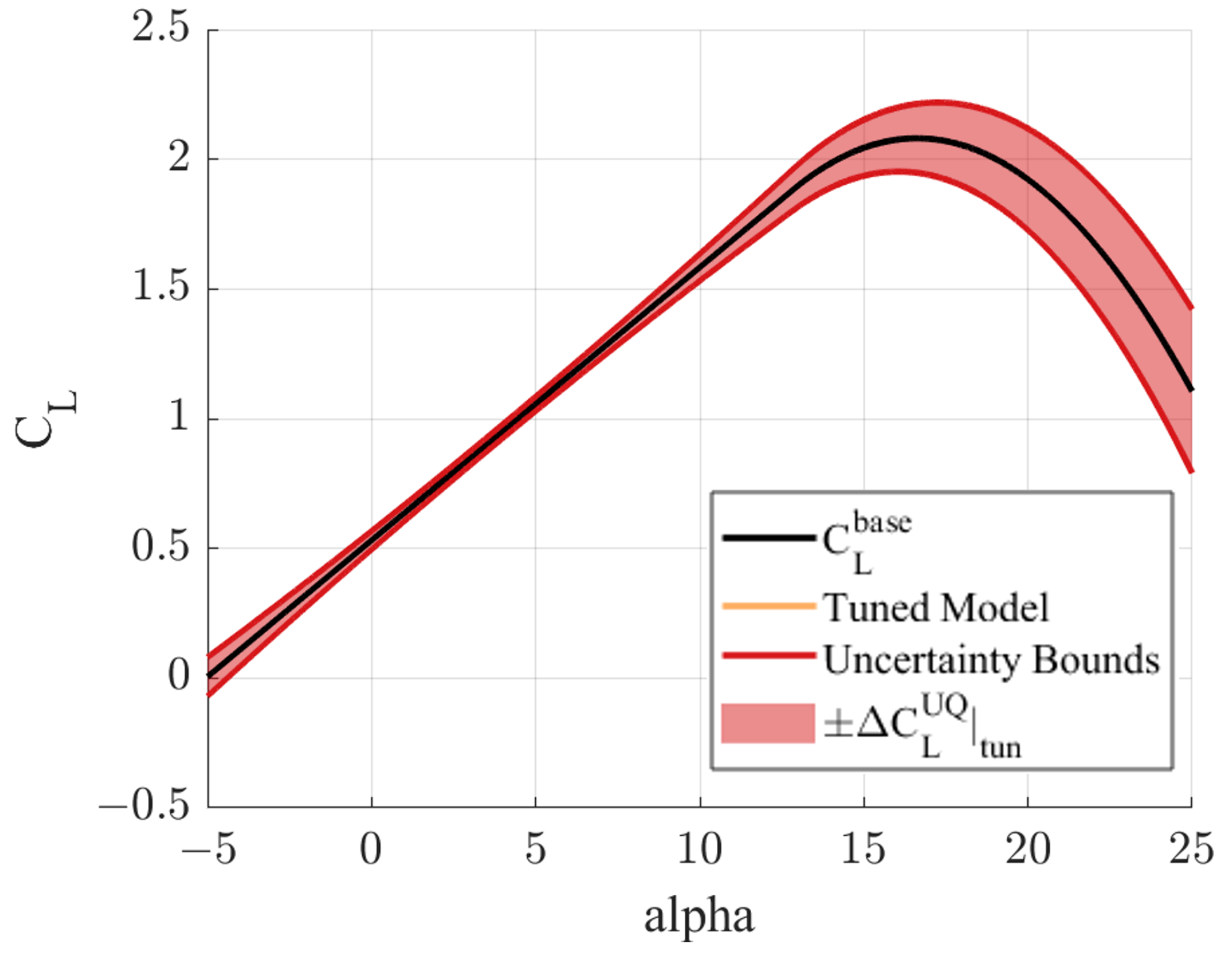
3.1. Uncertainty Estimation Method 1—Tuned Model Method

The first method to estimate the model and uncertainties of the modified configuration assumes that the total uncertainty for the modified configuration is equivalent to the uncertainty for the nominal configuration and that the model tuning for the nominal configuration also applies to the modified configuration. This is the same as assuming that no additional model tuning is needed for the modified configuration and the uncertainty bounds of the nominal configuration are valid for the modified configuration. This is a suitable assumption when the modification is small and has well-known and well-behaved aerodynamic effects. The determination of what constitutes a small modification is an area of future research.

In order to generate the updated model used for non-deterministic simulations, the final model can be written as

$$C_{*}=C_{*}^{base}+\Delta C_{*}^{tun}\pm \Delta C_{*}^{UQ}{|}_{tun}+\delta C_{*}^{base}$$

(6)

In other words, only the baseline model for the modified configuration is updated, i.e., corrected, using the change from the nominal configuration to the modified configuration ($\delta C_{*}^{base}$), as shown in Figure 5 using example artificial data. The uncertainty bounds for the nominal configuration ($\Delta C_{*}^{UQ}{|}_{tun}$), calculated using the tuned model, are then applied to this model to obtain updated uncertainty bounds for the modified configuration. This process is shown in Figure 6 for the example data.

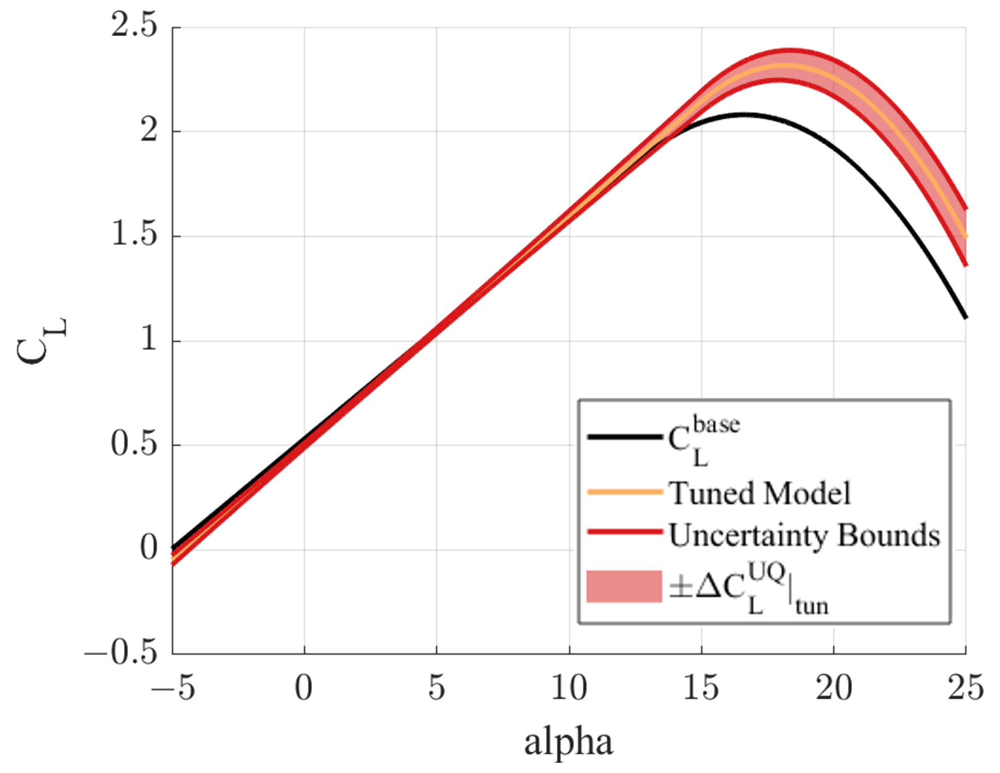
3.2. Uncertainty Estimation Method 2—Baseline Model Method

The second method of estimating the uncertainties of the modified configuration assumes that the total uncertainty for the modified configuration is the uncertainty that would occur if there were no tuning for the nominal configuration. This is equivalent to assuming the model tuning correction for the nominal configuration is no longer valid and approximating the total uncertainty for the modified configuration as the uncertainty for the nominal configuration with no tuning. Furthermore, it is assumed that the uncertainty bounds remain the same due to the similarity in configuration for the baseline modeling methods. The updated model for the modified configuration can then be written as

$$C_{*}=C_{*}^{base}\pm \Delta C_{*}^{UQ}{|}_{base}+\delta C_{*}^{base}$$

(7)

For this method, the baseline model for the nominal configuration has the change due to the modified configuration ($\delta C_{*}^{base}$) added to create the updated model, shown in Figure 7 with the example data. Then, uncertainty bounds ($\Delta C_{*}^{UQ}{|}_{base}$) created using flight test data and the baseline model of the nominal configuration, as opposed to the tuned model used for the Tuned Model Method, are used. This creates much larger uncertainty bounds that include the effects of model tuning, as in Figure 8.

3.3. Use of the Two Methods

The two methods of estimating the uncertainty for modified configuration are expected to provide different levels of conservativeness, depending on the characteristics of the model and configuration. The Tuned Model Method, which assumes that the tuning is valid and leads to smaller uncertainty for the updated model, effectively tunes the model based on the nominal configuration. This assumption will lead to less conservative uncertainty bounds about the updated model. An updated model and corresponding uncertainties based on the Tuned Model Method are accurate for modified configurations that are similar to the nominal configuration—i.e., the modifications are minor. However, the Baseline Model Method, which assumed a larger uncertainty that includes the tuning of the baseline model, is expected to give more conservative bounds that will account for larger differences between the nominal and modified configurations. This is akin to saying that the tuning correction from the nominal configuration no longer applies to the modified configuration because the changes are sufficiently large. However, the precise definition of what constitutes a sufficiently large modification is still an area of active research.

4. Uncertainty Estimation for an Example Aircraft System

The framework is demonstrated using an example aircraft system through the method of manufactured universes, which allows for the validation of uncertainty quantification methods using simulated data and uncertainties [20]. Because high-fidelity or flight test data are not always available for modified aircraft configurations, this approach allows for direct comparison between predicted results and the “true” system response. It also enables the evaluation of the impact of noise level and data quality on the framework and results.

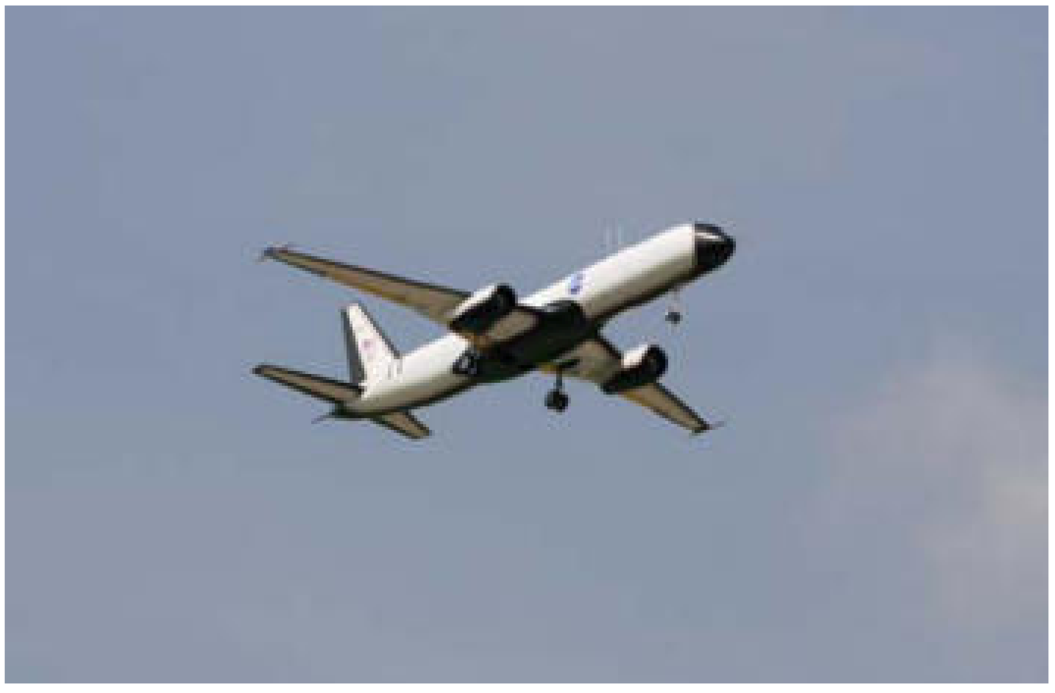
4.1. Example Aircraft System

NASA Langley Research Center’s Generic Transport Model (GTM) aircraft, shown in Figure 9, was chosen as the example aircraft system to demonstrate the proposed framework and methods. The GTM has had extensive wind tunnel, CFD, and flight tests and has been used for research including loss of control prediction, spin prediction, and control law development [25,26,27,28]. An open-source high-fidelity, non-linear simulation of the GTM (Available at: https://github.com/nasa/GTM_DesignSim (accessed on 1 August 2019)), created using a combination of a wind tunnel, flight test, and simulation data was used for this research.

The aircraft simulation was tuned using a constant true airspeed, which results in the trimmed aircraft states in

Table 1. GTM Trim States and Deflections.

State	Trim Value
u	50.2 m/s
v	0 m/s
w	2.59 m/s
p	0 rad/s
q	0 rad/s
r	0 rad/s
$\varphi$	0 rad (0 deg)
$\theta$	0.05 rad (2.86 deg)
Deflection	Trim Value
${\delta }_e$	2.45 deg
${\delta }_r$	0 deg
${\delta }_a$	−0.39 deg
${\delta }_T$	40.6%

. Although the GTM simulation environment includes many control inputs, only throttle, elevator, rudder, and aileron deflections were used for this research, with all other surfaces kept at the trimmed or zero position. All simulation and uncertainty results are shown as deviations from the trimmed aircraft state and surface deflections.

The simulation includes a Dryden atmospheric turbulence model, allowing for the simulation of flight test data with process noise. Sensor noise was also included in the simulation, using the included noise model of the sensors present in the flight test vehicle. Separate simulated flight test data segments were created for system identification, uncertainty quantification, and uncertainty validation. Because this is simulated data, flight test data can also be created for the modified configurations.

4.2. Model Definitions for Example Aircraft System

A baseline model of the GTM was created using the linearized longitudinal and lateral dynamics generated by the GTM simulation. This model serves as an approximation to CFD data and gives a lower fidelity aerodynamics model. A tuned model was created using the output error method to identify the system from simulated flight test data of independent elevator, rudder, and aileron doublets. A comparison of the baseline and tuned models to the observed flight test data is shown in Figure 10. The tuned model is much closer to the simulated flight test data than the baseline model, capturing the aircraft dynamics more accurately. These plots were generated by solving the following systems of equations for the baseline and tuned models, respectively:

$$\begin{array}{cc}\hfill {\dot{x}}^{base}& =A^{base}{x}^{base}+B^{base}{u}^{flighttest}\hfill \\ \hfill x_0^{base}& =x_0^{flighttest}\hfill \end{array}$$

(8)

and

$$\begin{array}{cc}\hfill {\dot{x}}^{tuned}& =A^{tuned}{x}^{tuned}+B^{base}{u}^{flighttest}\hfill \\ \hfill x_0^{tuned}& =x_0^{flighttest}\hfill \end{array}$$

(9)

where x is the aircraft states, the A and B matrices come from the baseline or tuned models, and the control inputs vector, u, is taken from the flight test data.

Uncertainties were then calculated using the error between the artificial flight test data and the baseline and tuned models, shown in Figure 11 and Figure 12, respectively. As described in Section 2, these uncertainties can vary with aircraft state, but must always include the potential for no uncertainty. Because the uncertainty is calculated about different models, the differences are expected. Since the uncertainty is added to the derivatives of the states, even a small difference can have a large effect in the performance estimation. If the performance is to be estimated at a higher velocity or at a combination of angular rates, these states should be included in the data used for uncertainty quantification. If representative flight test data are not used in the calculation, the bounds will not adequately estimate the model form uncertainty. For this reason, the simulated flight test data used for uncertainty quantification included a combination of aircraft velocities, angular rates, and control deflections. Although these bounds are generated using 95% confidence intervals, some flight test data points appear to lie outside the bounds due to slicing the multi-dimensional space to be shown in a two-dimensional figure plane.

Three example modified configurations were also created. The first modification is a 10% increase in the aircraft mass, distributed equally, while the second modification is a 10% increase in the aircraft mass alongside a small change in aircraft center of gravity location, and the third modification is a 10% increase in aircraft mass alongside a larger change in aircraft center of gravity location. The first modification, with equally distributed mass, does not change the relationship between the moments of inertia and can therefore be modeled by the simple linear model. The second and third modifications, with a change to the center of gravity location, will cause changes to the moments of inertia that are not modeled. Although these modifications are not necessarily realistic, they serve to illustrate the methods and frameworks with both modeled and un-modeled modifications.

4.3. Uncertainty Estimation Methods for Example Aircraft System

The uncertainty estimation methods described in Section 2 were evaluated using the models and simulated flight test data for the modified GTM aircraft configurations. To do so, thousands of non-deterministic simulations were conducted, which solve the following system of equations, which includes the estimated uncertainty evaluated at each timestep as a function of the aircraft state.

$$\begin{array}{cc}\hfill {\dot{x}}^{updated}& =A^{updated}{x}^{updated}+B^{updated}{u}^{flighttest}+U{Q}^{updated}{|}_x\hfill \\ \hfill x_0^{updated}& =x_0^{flighttest}\hfill \end{array}$$

(10)

where x is the aircraft states, the A and B matrices come from the updated model, the control inputs vector, u, comes from the flight test data, and the uncertainty, $UQ$ comes from the updated uncertainty estimation evaluated for the given aircraft states at each timestep.

The performance bounds, in red, are then calculated by taking the 95% bounds of these compiled simulations. Figure 13 shows the resulting updated model and associated uncertainty bounds for the Tuned Model Method, while Figure 14 shows the results for the Baseline Model Method evaluated for the equally distributed mass modification. Due to the calculation in the updated model for each method, there are slight differences in the results for the updated model without the uncertainty. The Baseline Model Method also generates larger uncertainty bounds, most notably in the downward velocity ($\Delta w$) and yaw rate ($\Delta r$). The uncertainty in the forward velocity ($\Delta u$) is large in both methods, due to the large effects of the ignored non-linear dynamics.

5. Validation of Framework for an Example Aircraft System

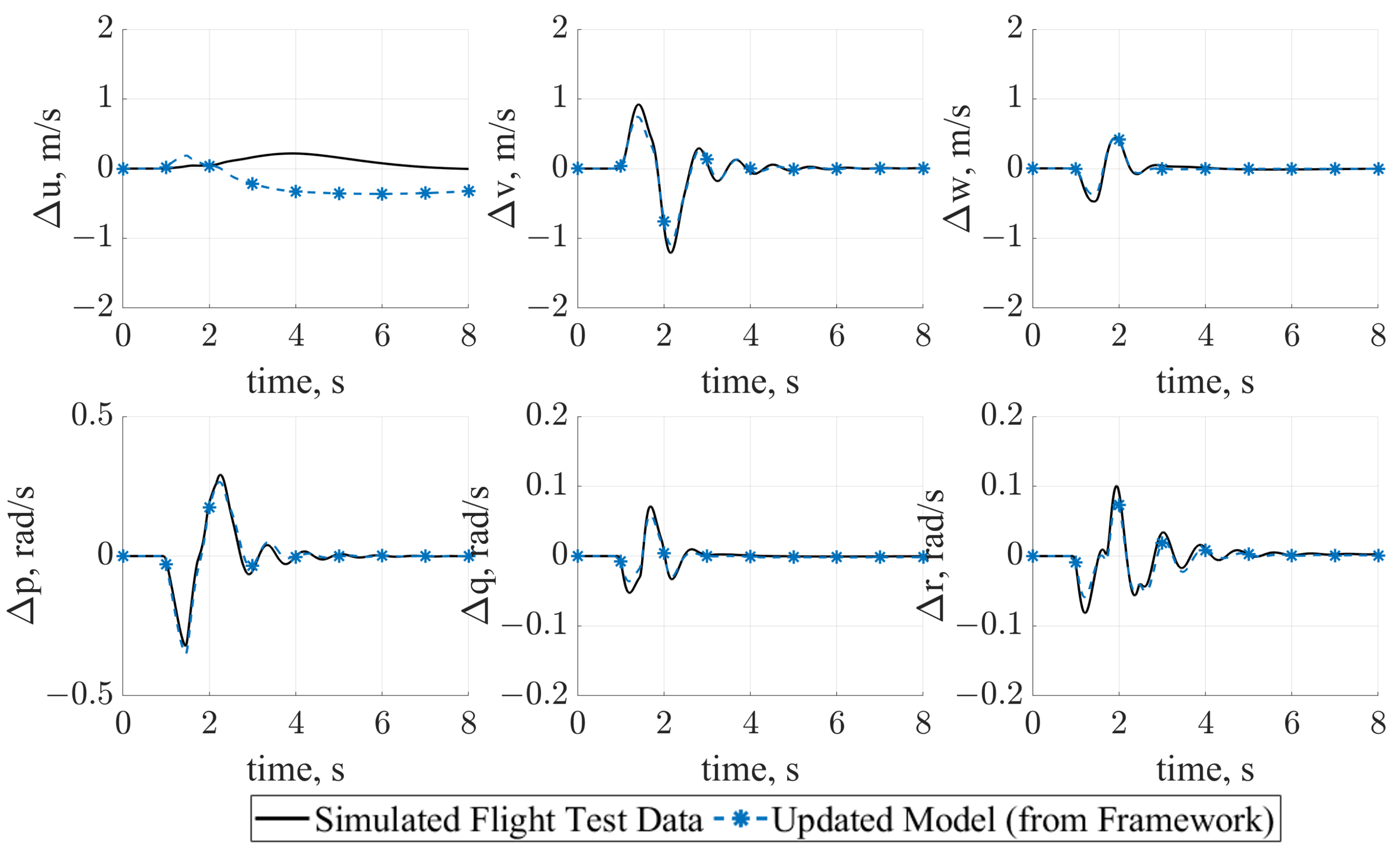
5.1. Validation of Performance Estimation without Noise

Before validating the performance of the framework for a realistic case with both wind and signal noise, the no noise, no wind case was studied. Because these noise sources are included in the estimation of model form uncertainty, the no noise case allows evaluation of the framework with the most accurate estimation of uncertainty.

The tuned model for the nominal, unmodified configuration, closely matches the simulated flight test performance, as calculated using Equation (9), shown in Figure 15. For most of the aircraft states, the updated model correctly predicts the flight test performance, with the exception of the forward velocity, $\Delta u$. Forward velocity often has larger deviations in simulation and modeling due to non-linear terms that are excluded.

When the Tuned Model Method is extended to a modified configuration, in this case, the 10% increase in mass, the results remain in good agreement with the simulated flight test data. Figure 16 shows the comparison of the two, with the updated model generated using the Tuned Model Method in blue. There are distinct differences between the two, notably that the updated model has increased damping relative to the simulated flight test data and does not have the same peak magnitude in the velocity perturbations.

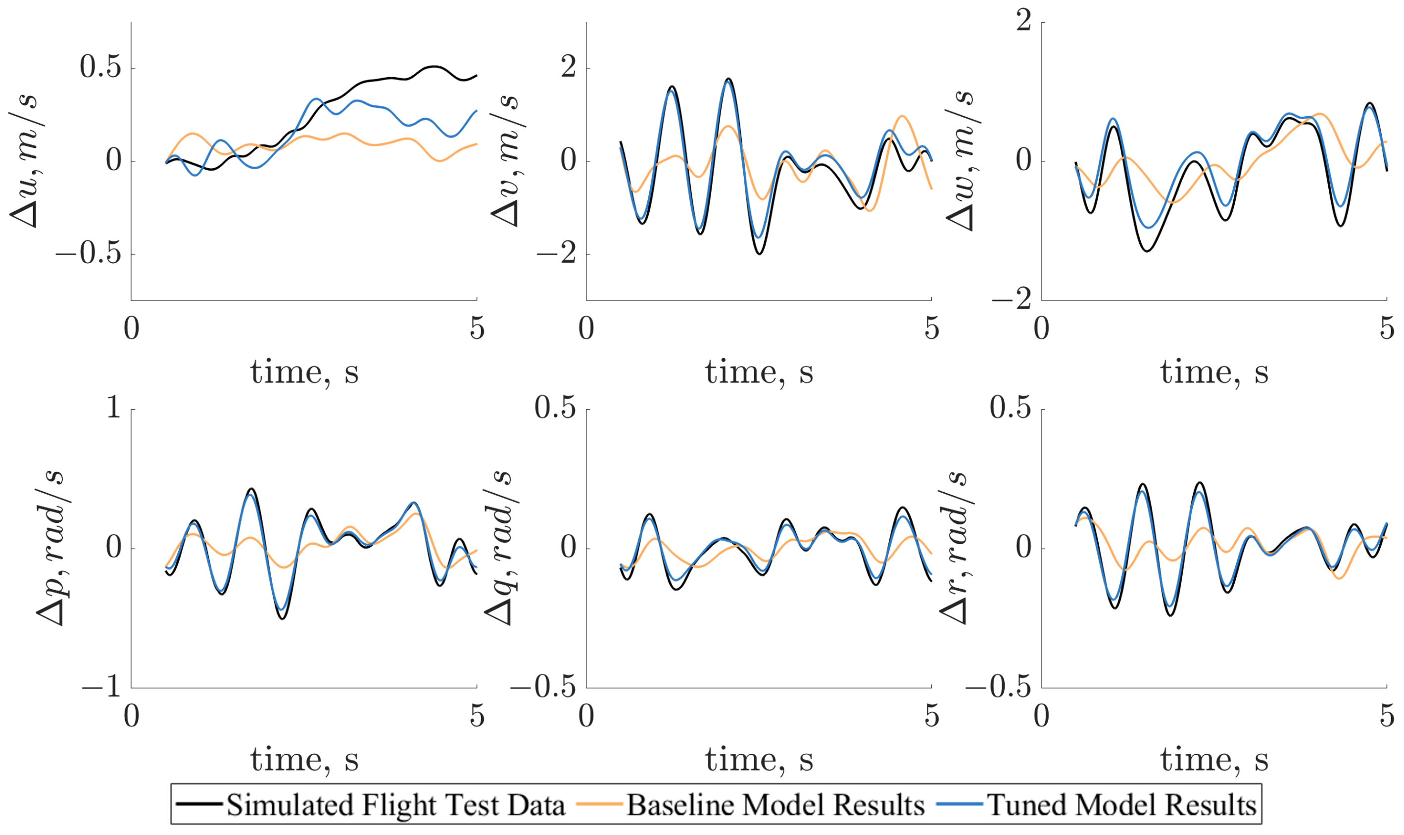
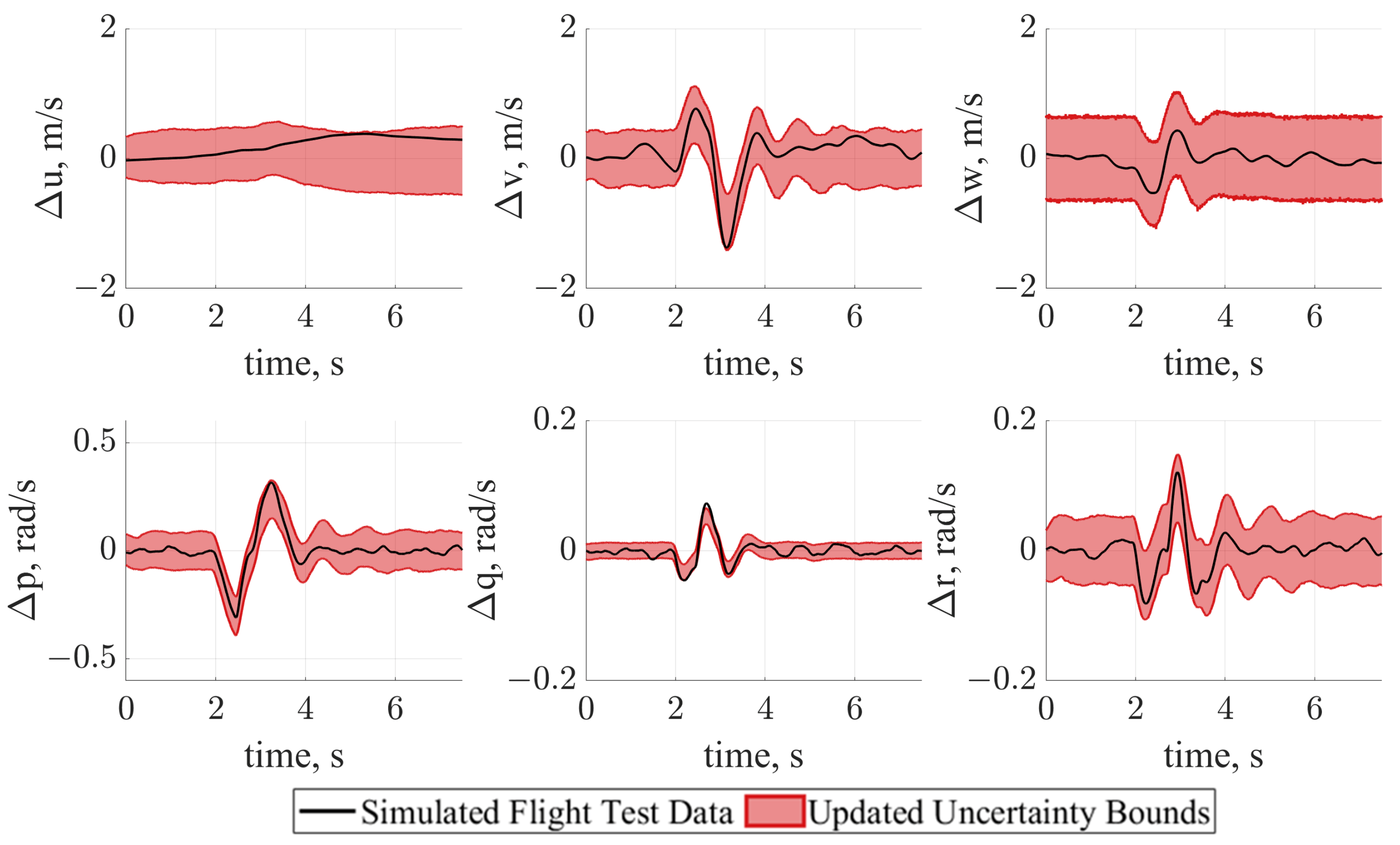
5.2. Validation of Performance Estimation

The uncertainty bounds generated from evaluating the Tuned Model Method and Baseline Model Method using Equation (10) were then compared to the simulated flight test data for the three different modifications, for a separate validation maneuver. To evaluate the performance of the framework, the percentage of simulated flight test data falling within the estimated uncertainty bounds is calculated by evaluating whether each time step falls within the bounds, for all states. This metric counts each state independently, so a timestep which is outside the bounds for multiple states would each have a negative impact. For the first modification of an equally distributed increase in mass, the uncertainty bounds generated contain the simulated flight test data for 94% of the data points, as shown in Figure 17. This provides evidence that the method can correctly predict the performance of this configuration in a realistic scenario with both wind and sensor noise.

However, when these generated bounds are compared to the simulated flight test data for the second modification, of an unequally distributed mass with change in center of gravity location, the performance bounds only contain the simulated flight test data for 77% of the simulated flight test data points, shown in Figure 18. The mismatch, most noticeable in downward velocity $\Delta v$ and pitch rate $\Delta q$, is because the modification is not sufficiently represented by the lower fidelity models used to generate the uncertainty bounds, specifically the un-modeled change in moments of inertia. For these situations, the Baseline Model Method generates larger uncertainty bounds to capture more of the dynamics of the modified configurations. For the modification of the unequally distributed mass, the Baseline Model Method does capture more of the simulated flight test data, particularly the high angular rates, containing approximately 98% of the simulated flight test data points, as shown in Figure 19. This significant increase is due to the larger estimated uncertainty bounds calculated with the Baseline Model Method, which is designed to be able to predict the performance of larger modifications.

As a further extension, these methods were applied to a modification with a 10% mass increase, but a much larger change in center of gravity location (Modification 3). When the Tuned Model Method was applied to this modification, the estimated performance bounds contained the simulated flight test data for only 19% of the data points, shown in Figure 20. When the Baseline Model Method is applied to this configuration, illustrated in Figure 21, the estimated performance bounds contain the simulated flight test data for 21% of the data points, a slight improvement but still significantly less than the previous configurations. The range of applicability of the uncertainty estimation methods is an area of active research.

Table 2. Comparison of Estimated Performance Bounds Metric for GTM Modifications.

Modification	Tuned Model Method	Baseline Model Method
10% Increase in Mass	94%	—
10% Increase in Mass and Change In CG	77%	98%
10% Increase in Mass and Large Change In CG	19%	21%

contains a summary of the results presented in this section, demonstrating the improvement in the amount of data points contained within the estimated performance bounds for the Baseline Model Method for the larger modifications and the small amount of data points contained when the two methods were used to estimate the performance of the configuration with a 10% mass increase with large change in center of gravity location.

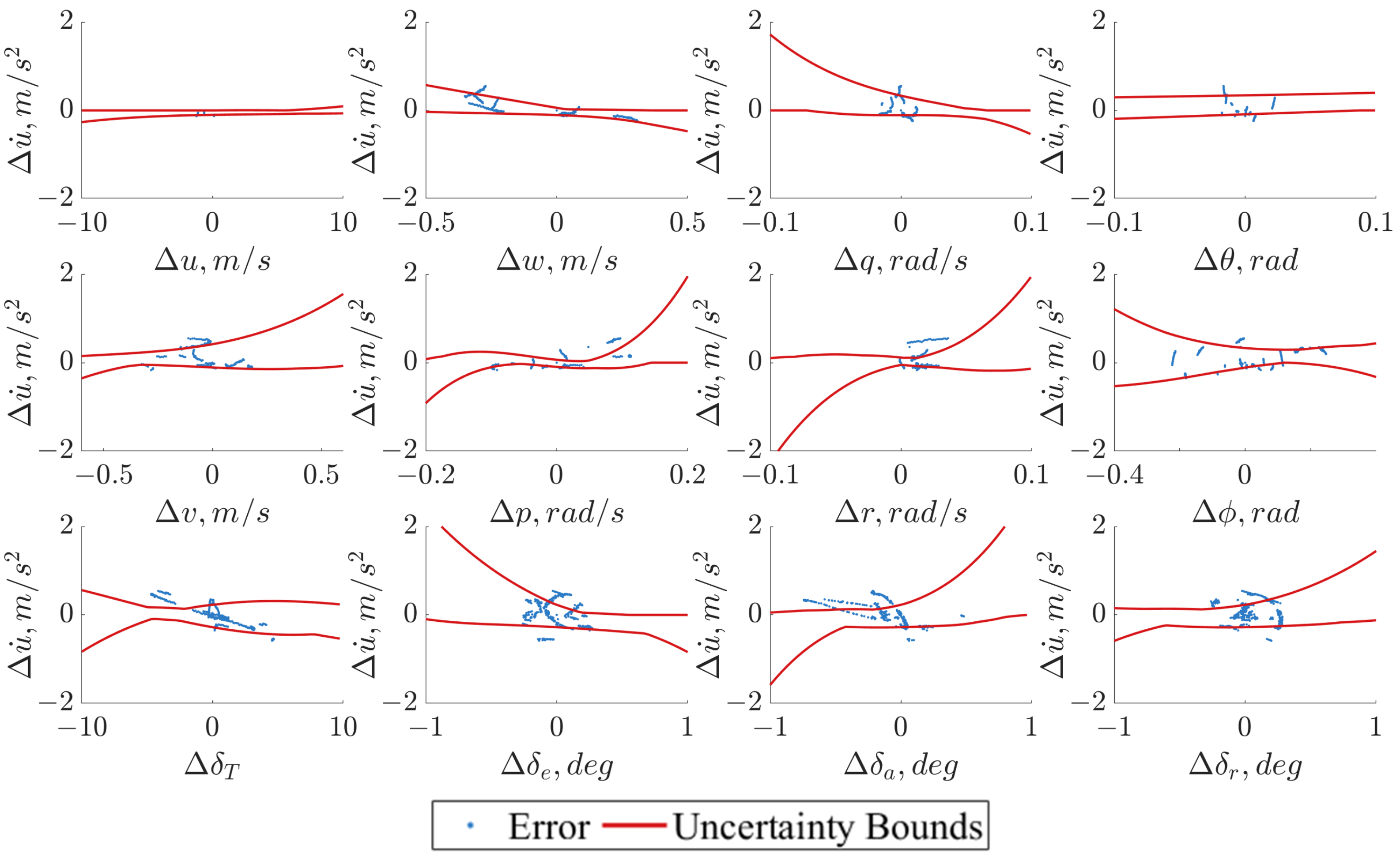
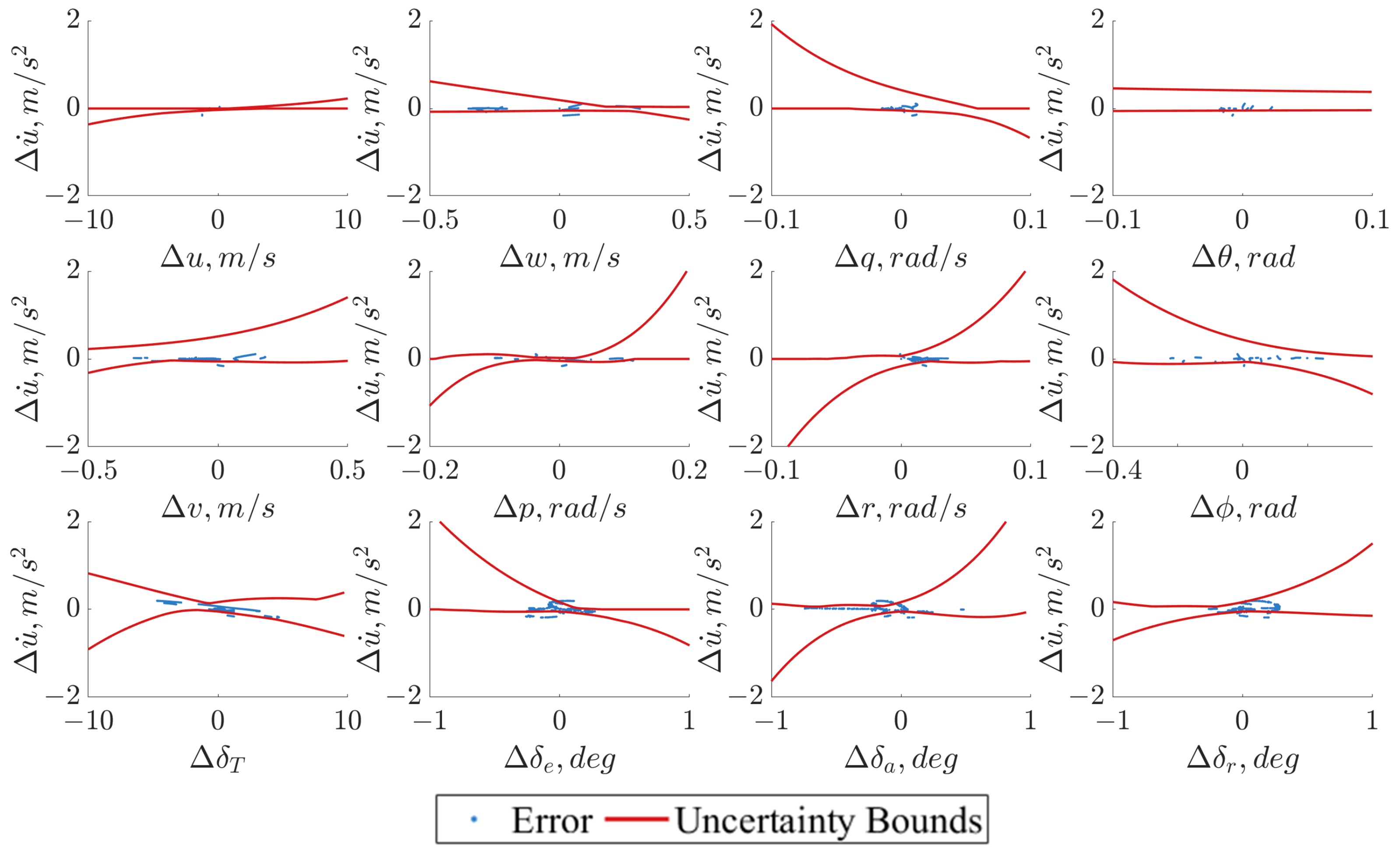
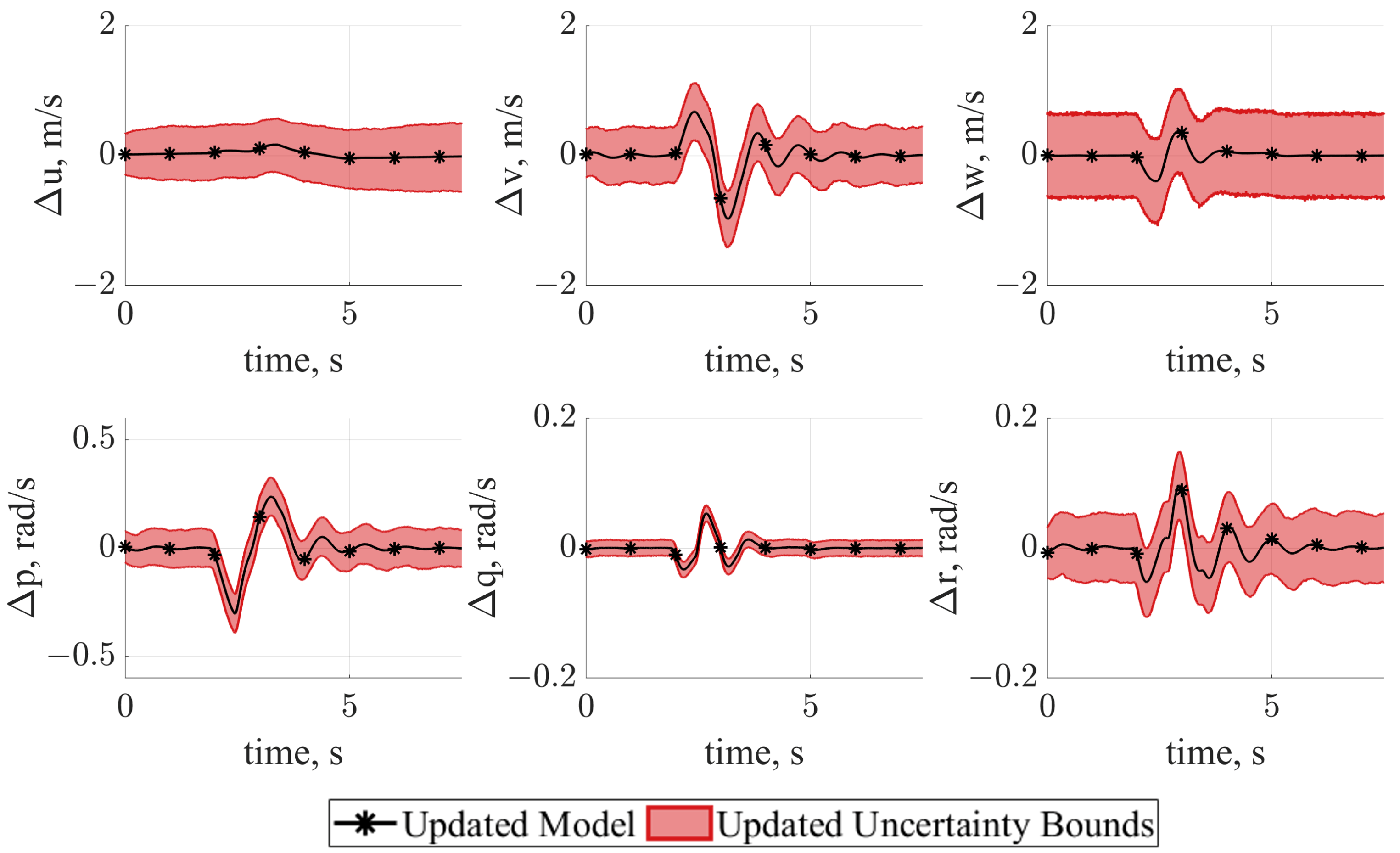
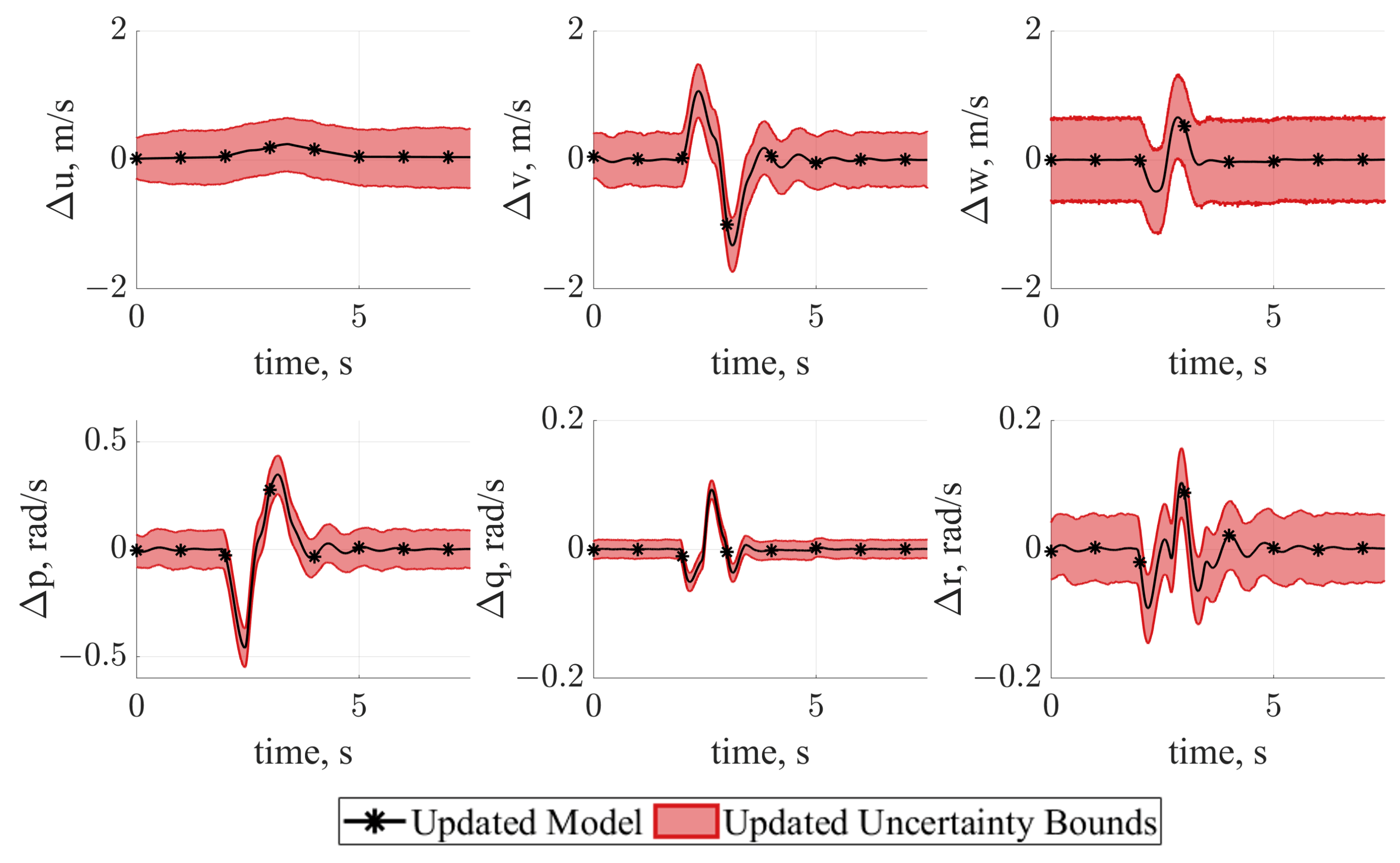
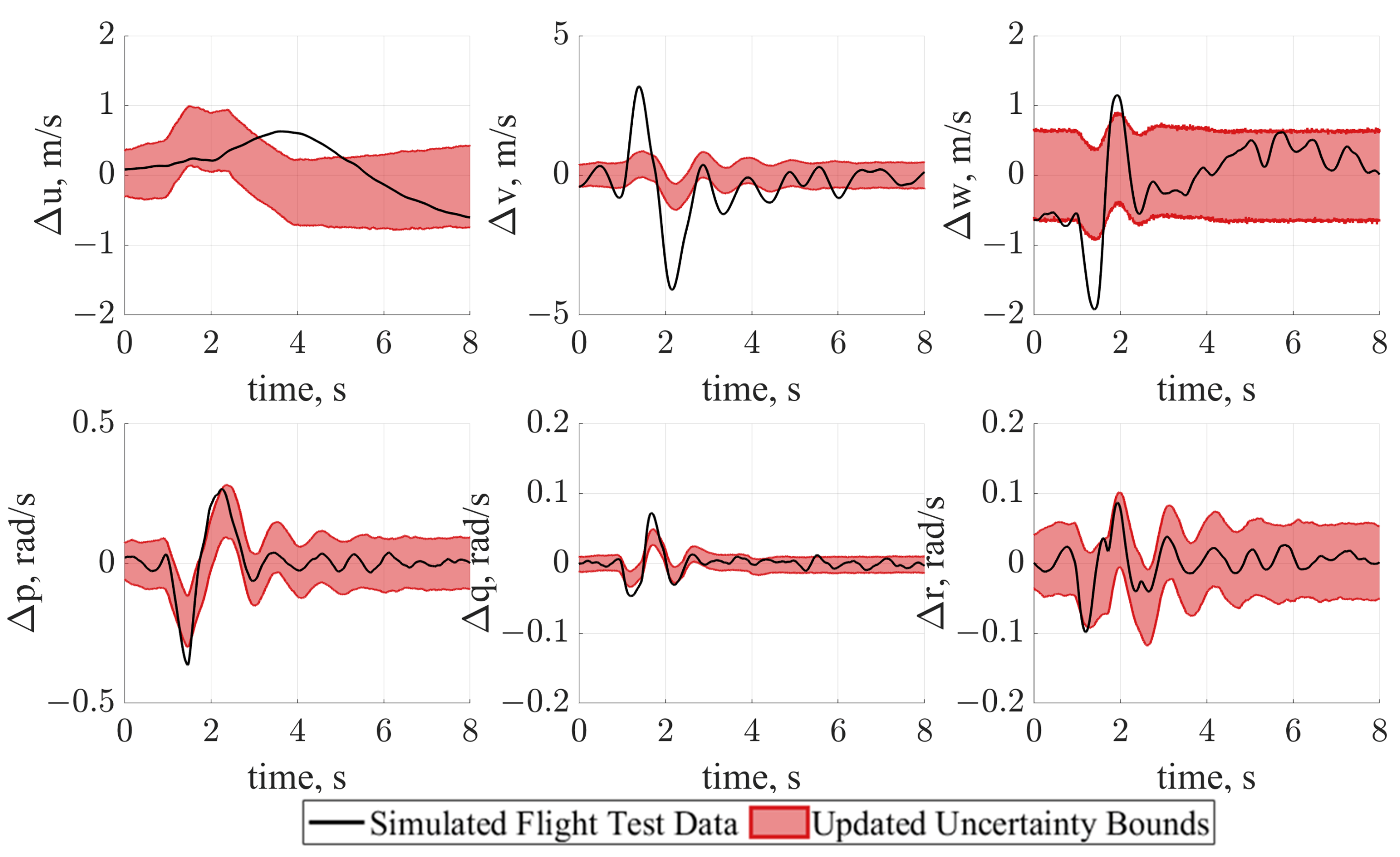
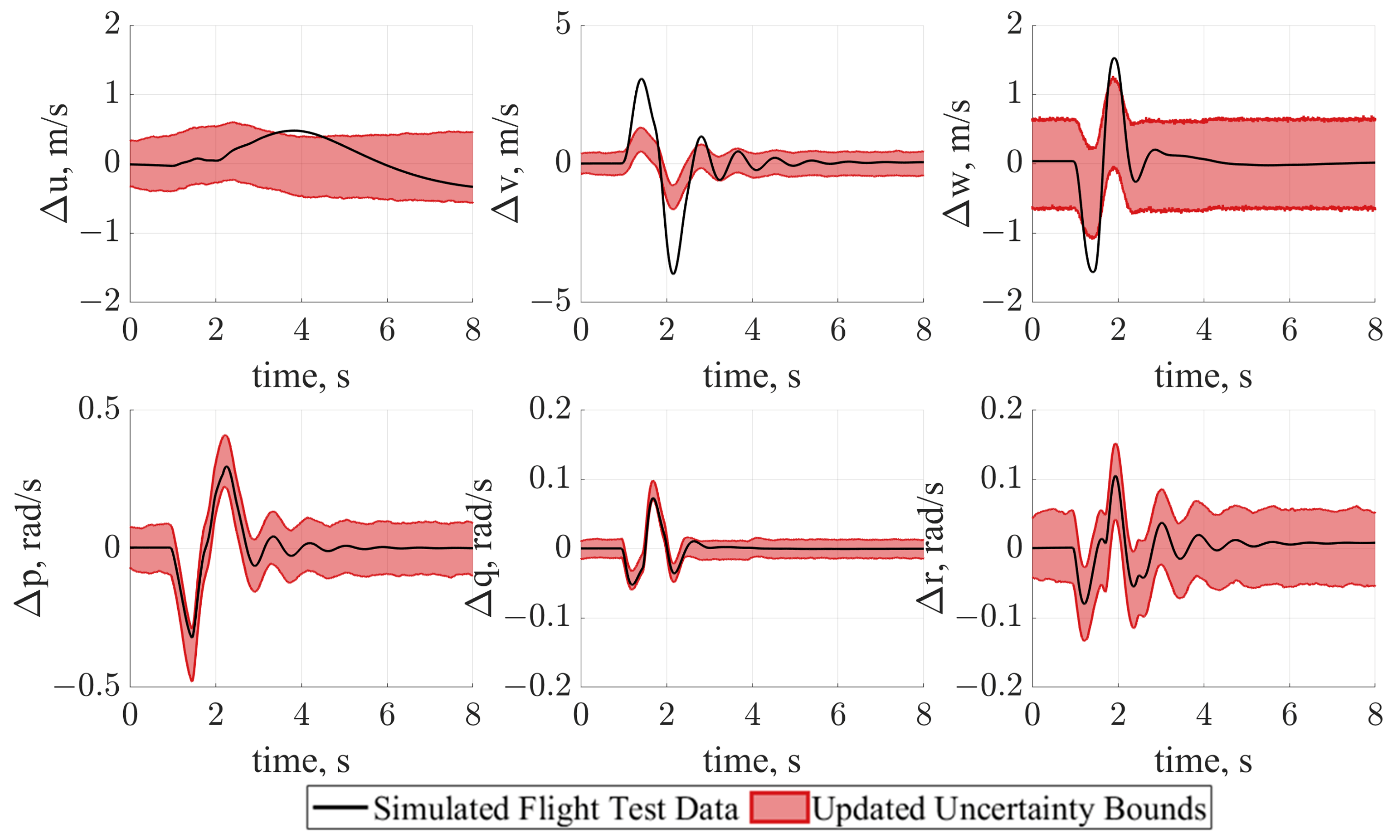
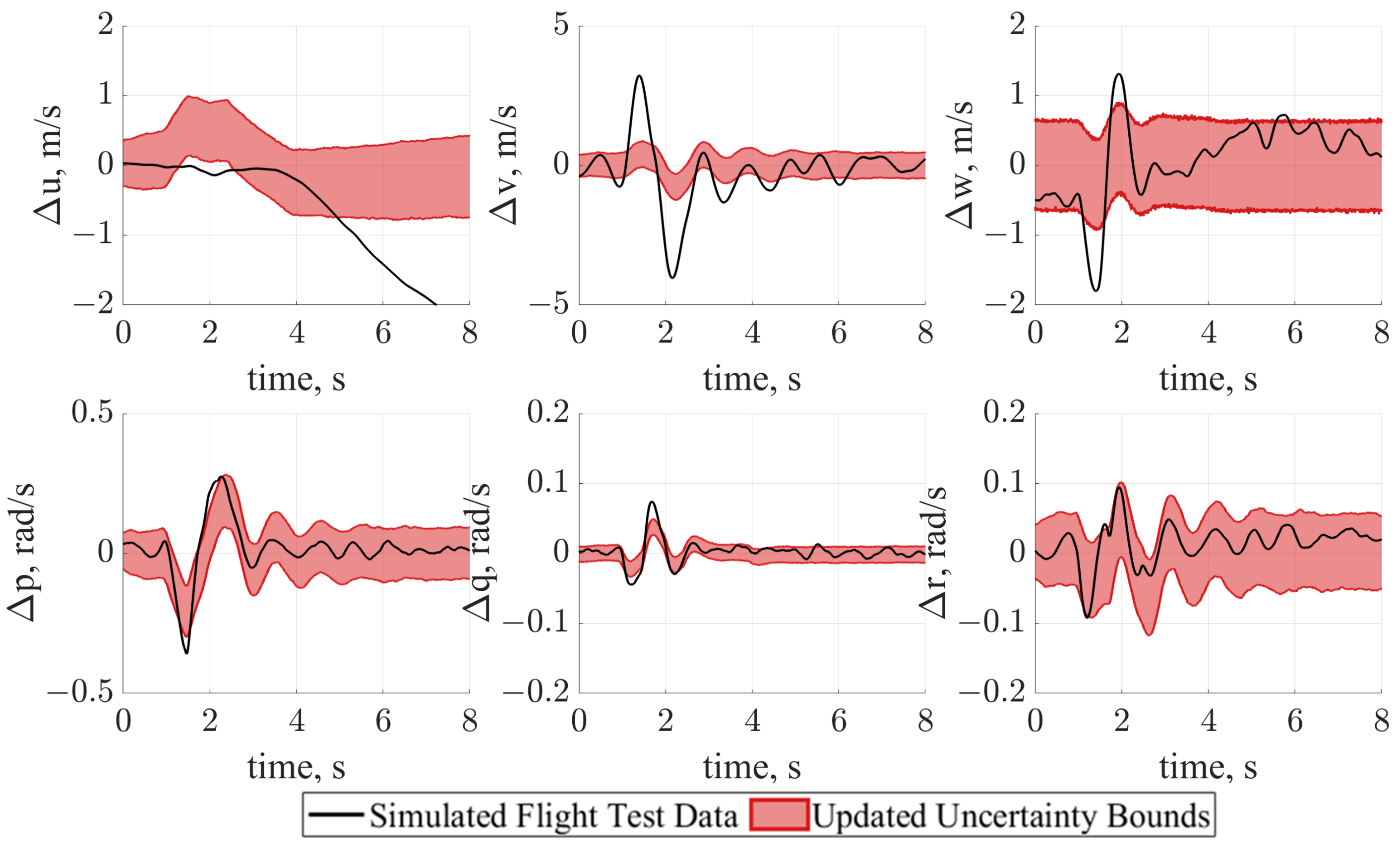
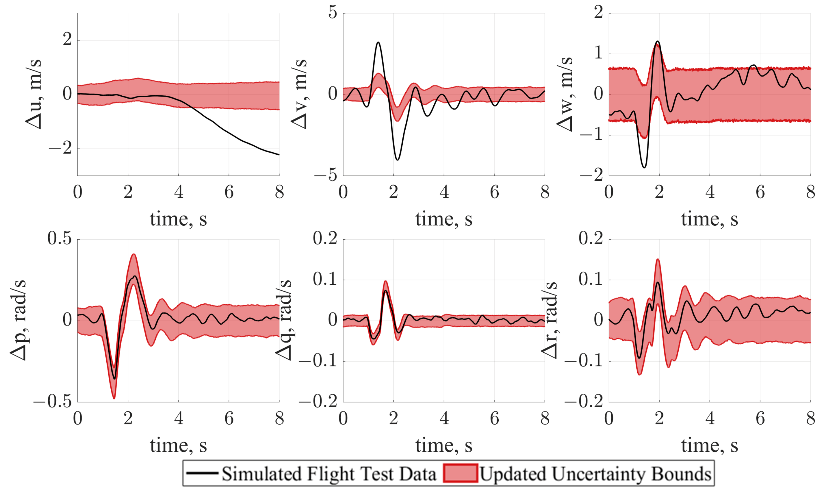
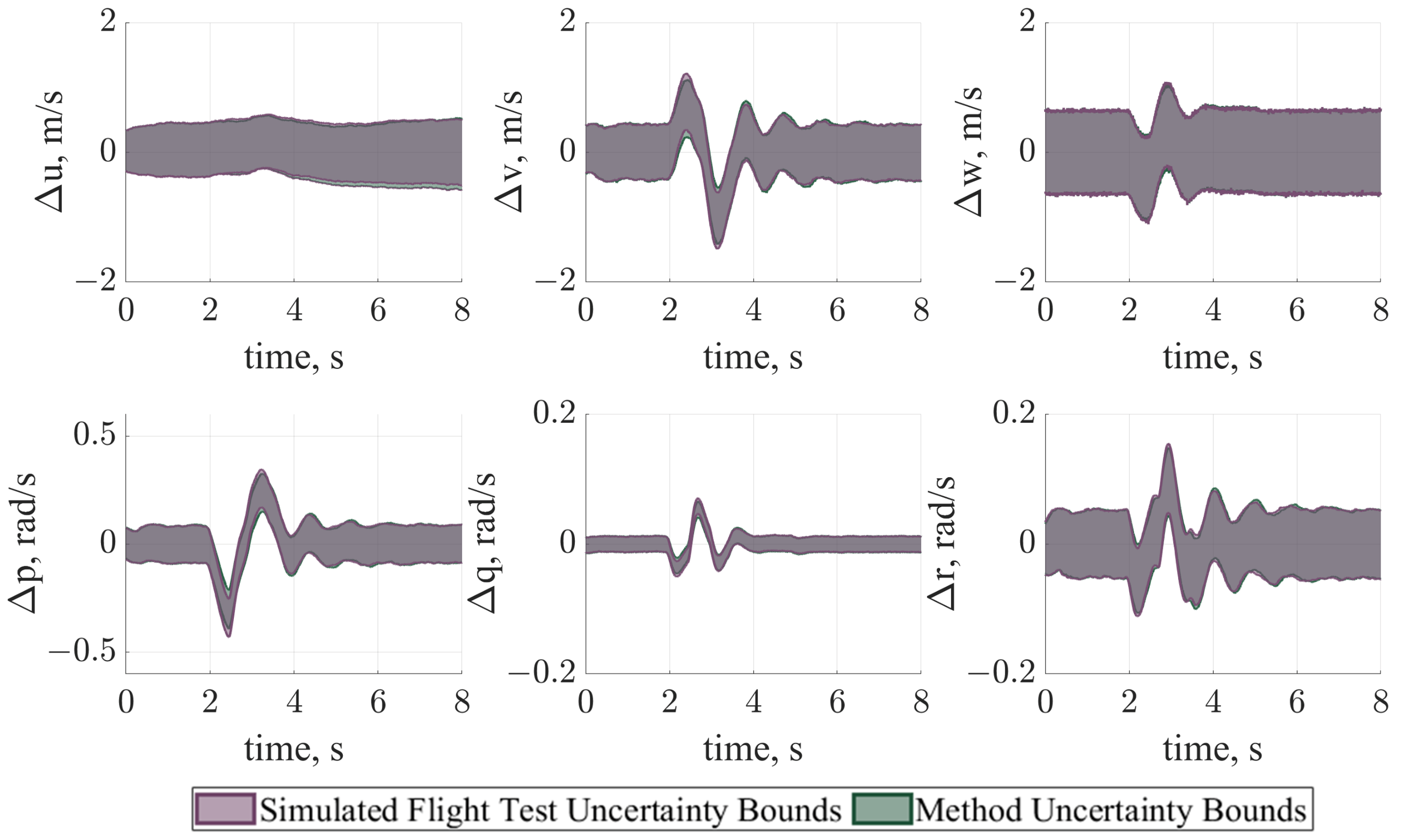
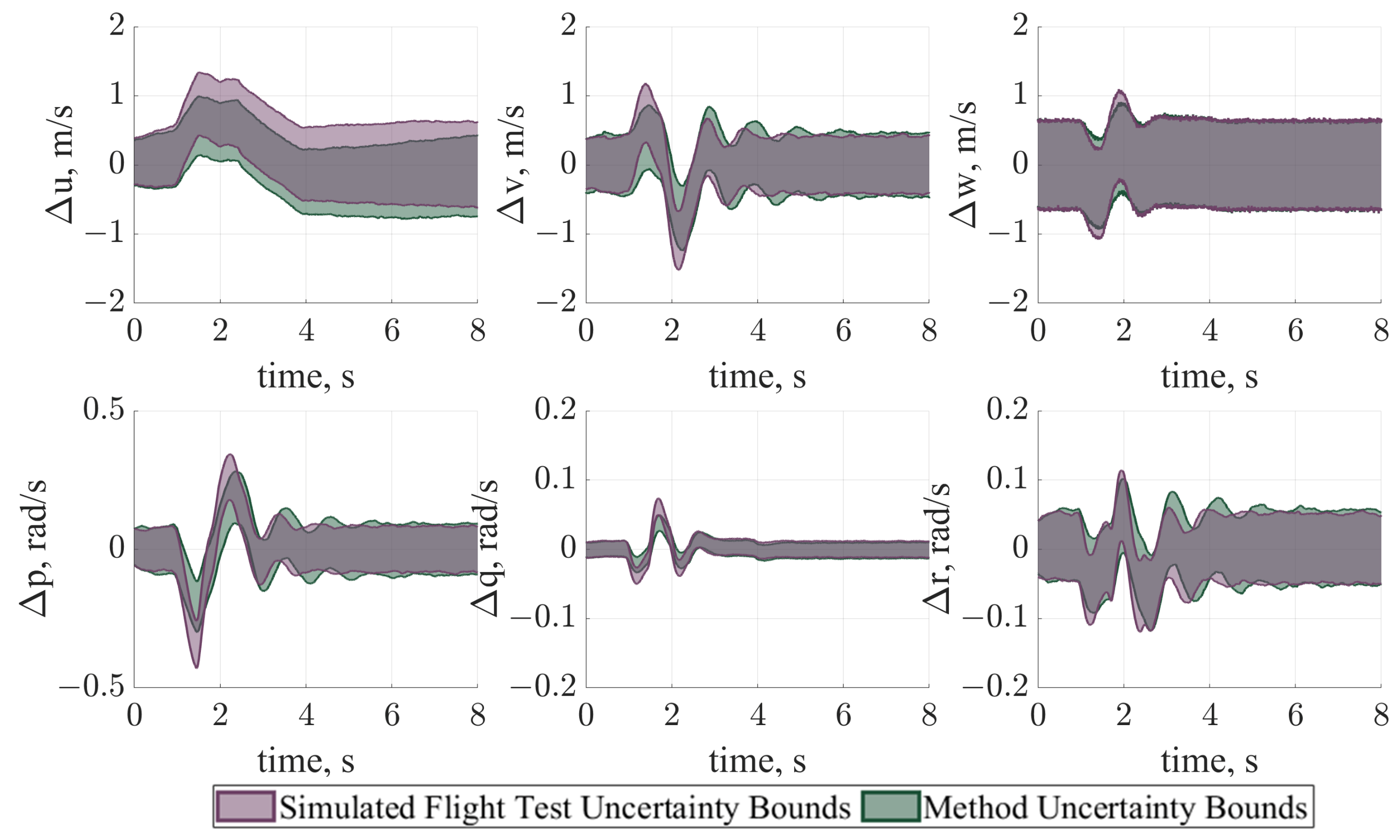
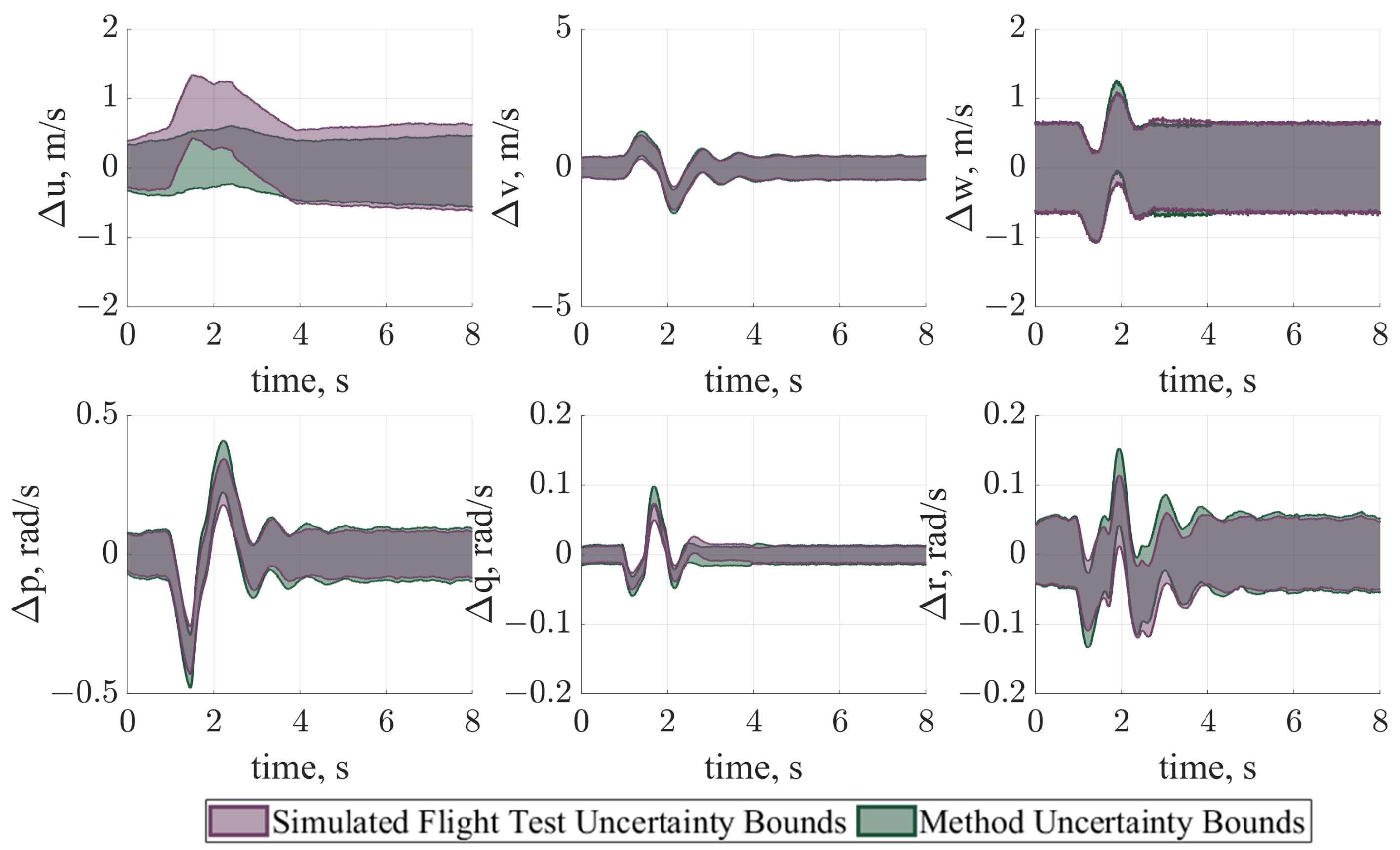
5.3. Validation of Uncertainty Estimation Methods

Along with estimating the performance of modified aircraft configurations, estimating the model form uncertainty for a higher fidelity model of this configuration can also aid the certification process. Because we are using simulated flight test data, it is possible to obtain flight test data for the modified configurations that would otherwise be unavailable. Using the same uncertainty estimation method described in Section 2, the true uncertainty for the modified configuration can be calculated. For the first modification of equally distributed mass, the estimated performance bounds generated by the Tuned Model Method are quite similar to the uncertainty bounds calculated by simulating the actual modified configuration, shown in Figure 22. For most of the maneuver, the two bounds are almost identical.

However, when the Tuned Model Method is used to estimate the uncertainty bounds for the distributed mass configuration with change to the center of gravity location, as shown in Figure 23, the estimated uncertainty bounds are significantly different than the true uncertainty bounds, particularly in the forward velocity, $\Delta u$, but with differences in the other states. The estimated uncertainty bounds generated using the Baseline Model Method show an improvement, capturing more of the overall trend and magnitude of the uncertainty bounds calculated from the modified configuration, seen in Figure 24.

6. Summary and Conclusions

A framework to estimate the performance and associated uncertainty bounds for modified aircraft configurations without requiring flight test or other high fidelity data of the modified configuration is introduced. This framework includes two methods to estimate the uncertainty of the modified configurations based on the uncertainty calculated for the nominal configuration. The first uncertainty estimation method, the Tuned Model Method, assumes that the model tuning for the nominal configuration is still valid for the modified configuration and that no additional uncertainty is introduced, whereas the second method, the Baseline Model Method, does not make this assumption and calculates larger uncertainty bounds relative to the baseline model in order to capture more of the modification dynamics. These methods are designed independently of the data collection method (wind tunnel, CFD, simulation, or flight test) as well as the model form (linear, non-linear) of the aircraft model.

These methods are then applied using data from the Generic Transport Model (GTM), a research aircraft operated by NASA Langley. A high-fidelity simulation is used to create simulated flight test data as well as linearized models. Three modifications are examined, the addition of an equally distributed mass, the addition of a distributed mass with a small change in center of gravity location, and the addition of a distributed mass with a larger change in center of gravity location. The equally distributed mass is modeled in the baseline model, whereas the two mass distributions with changes in center of gravity locations is not fully captured using the linear model by neglecting the changes in the moments of inertia.

The Tuned Model Method is adequate at predicting both the performance and uncertainty of the equally distributed mass modification but does not fully capture the performance or uncertainty for the modification with a mass increase and a small change in the center of the gravity location. The Baseline Model Method better captures the performance of this modification and provides a more accurate uncertainty profile. Although the results are not as accurate for the case where there is a mass increase and a much larger change in center of gravity location, the differences could indicate that the framework is not applicable for this large of a modification because the uncertainty in the moments of inertia of this modified configuration is not captured by the uncertainty estimate.

The ability of the framework to predict the performance and associated uncertainty bounds of modified aircraft configurations without requiring flight test data of the modifications could have a significant impact on future certification by analysis work. Two current barriers to certification by analysis are the certainty that the calculated results are the same level of accuracy as flight test data and that the uncertainty in the calculated results is quantified. This framework addresses both concerns, providing a critical step towards certification by analysis.

Additional work includes further defining the range of applicability of the framework and the two included methods, both in terms of size and type of aircraft modifications. The range of applicability of these methods is especially important when considering the use of this framework to supplement or reduce flight testing or when considering certification by analysis. These methods will also be applied to NASA’s X-57 Maxwell aircraft, which already incorporates several modifications. By using a manned aircraft, the performance predictions can be directly applied to existing airworthiness certification criteria, enabling evaluation of the methods to predict aircraft performance at a suitable level.

References

1. Lucka, D.A. Refining the U.S. Navy Flight Clearance (Airworthiness Certification) Process: Maximizing Acquisition Reform Benefits for Commercial Derivative Aircraft Acquisitions. Master’s Thesis, University of Tennessee, Knoxville, TN, USA, 2003. [Google Scholar]
2. Flight Clearance Policy for Air Vehicles and Aircraft Systems; NAVARINST 13034.1D; Naval Air Systems Command: Patuxent River, MD, USA, 2010.
3. Standard Airworthiness Certification Regulations; Federal Aviation Administration: Washington, DC, USA, 2021.
4. American Institute of Aeronautics and Astronautics (Ed.) Recommended Practice: When Flight Modelling Is Used to Reduce Flight Testing Supporting Aircraft Certification; AIAA R-154-2021; American Institute of Aeronautics and Astronautics, Inc.: Reston, VA, USA, 2021. [Google Scholar] [CrossRef]
5. Schaefer, J.A.; Romero, V.J.; Schafer, S.R.; Leyde, B.; Denham, C.L. Approaches for Quantifying Uncertainties in Computational Modeling for Aerospace Applications. In Proceedings of the AIAA Scitech 2020 Forum; Orlando, FL, USA, 6–10 January 2020, AIAA 2020-1520; American Institute of Aeronautics and Astronautics: Orlando, FL, USA, 2020. [Google Scholar] [CrossRef]
6. National Research Council (Ed.) Evaluation of Quantification of Margins and Uncertainties Methodology for Assessing and Certifying the Reliability of the Nuclear Stockpile; National Academies Press: Washington, DC, USA, 2009. [Google Scholar] [CrossRef]
7. Mehta, U.B.; Eklund, D.R.; Romero, V.J.; Pearce, J.A.; Keim, N.S. Simulation Credibilty—Advances in Vertification, Validation, and Uncertainty Quantification; Number NASA TP-2016-219422; National Aeronautics and Space Administration: Washington, DC, USA, 2016. [Google Scholar]
8. Roy, C.J.; Oberkampf, W.L. A Comprehensive Framework for Verification, Validation, and Uncertainty Quantification in Scientific Computing. Comput. Methods Appl. Mech. Eng. 2011, 200, 2131–2144. [Google Scholar] [CrossRef]
9. Roy, C.J.; Balch, M.S. A Holistic Approach to Uncertainty Quantification with Application to Supersonic Nozzle Thrust. Int. J. Uncertain. Quantif. 2012, 2, 363–381. [Google Scholar] [CrossRef]
10. Oberkampf, W.; Helton, J.; Sentz, K. Mathematical Representation of Uncertainty. In AIAA Applied Aerodynamics Conference; AIAA 2001-1645; American Institute of Aeronautics and Astronautics: Anaheim, CA, USA, 2001. [Google Scholar] [CrossRef]
11. Oberkampf, W.L.; DeLand, S.M.; Rutherford, B.M.; Diegert, K.V.; Alvin, K.F. Error and Uncertainty in Modeling and Simulation. Reliab. Eng. Syst. Saf. 2002, 75, 333–357. [Google Scholar] [CrossRef]
12. Schaefer, J.A.; Cary, A.W.; Duque, E.P.; Lawrence, S. Application of a CFD Uncertainty Quantification Framework for Industrial-Scale Aerodynamic Analysis. In AIAA Scitech 2019 Forum; AIAA 2019-1492; American Institute of Aeronautics and Astronautics: San Diego, CA, USA, 2019. [Google Scholar] [CrossRef]
13. Wendorff, A.D.; Alonso, J.J.; Bieniawski, S.R. A Multi-Fidelity Approach to Quantification of Uncertainty in Stability and Control Databases for use in Stochastic Aircraft Simulations. In Proceedings of the 16th AIAA/ISSMO Multidisciplinary Analysis and Optimization Conference, Dallas, TX, USA, 22–26 June 2015; AIAA 2015-3439. American Institute of Aeronautics and Astronautics: Dallas, TX, USA, 2015. [Google Scholar] [CrossRef]
14. Fidkowski, K.; Kroo, I.; Willcox, K.; Engelson, F. Stochastic Gust Analysis Techniques for Aircraft Conceptual Design. In Proceedings of the 12th AIAA/ISSMO Multidisciplinary Analysis and Optimization Conference, Victoria, BC, Canada, 10–12 September 2008; American Institute of Aeronautics and Astronautics: Victoria, BC, Canada, 2008. [Google Scholar] [CrossRef] [Green Version]
15. Ng, L.W.T.; Willcox, K.E. Monte Carlo Information-Reuse Approach to Aircraft Conceptual Design Optimization Under Uncertainty. J. Aircr. 2016, 53, 427–438. [Google Scholar] [CrossRef]
16. Steinkellner, S. Aircraft Vehicle Systems Modeling and Simulation under Uncertainty. Master’s Thesis, Linköping University Institute of Technology, Linköping, Sweden, 2011. [Google Scholar]
17. Hale, L.E.; Patil, M.; Roy, C.J. Nondeterministic Simulation for Probability of Loss of Control Prediction for Unmanned Aircraft Systems. In Proceedings of the AIAA Modeling and Simulation Technologies Conference, Dallas, TX, USA, 22–26 June 2015. AIAA 2015-2329. [Google Scholar] [CrossRef]
18. Hale, L.E.; Patil, M.; Roy, C.J. Aerodynamic Parameter Identification and Uncertainty Quantification for Small Unmanned Aircraft. In Proceedings of the AIAA Guidance, Navigation, and Control Conference, Kissimmee, FL, USA, 5–9 January 2015; AIAA 2015-1538. American Institute of Aeronautics and Astronautics: Kissimmee, FL, USA, 2015. [Google Scholar] [CrossRef]
19. Maine, R.E.; Iliff, K.W. The Theory and Practice of Estimating the Accuracy of Dynamic Flight-Determined Coefficients; NASA RP-1077; National Aeronautics and Space Administration: Washington, DC, USA, 1981. [Google Scholar]
20. Stripling, H.; Adams, M.; McClarren, R.; Mallick, B. The Method of Manufactured Universes for Validating Uncertainty Quantification Methods. Reliab. Eng. Syst. Saf. 2011, 96, 1242–1256. [Google Scholar] [CrossRef]
21. Jategaonkar, R.V. Flight Vehicle System Identification: A Time-Domain Methodology, 2nd ed.; Number 245 in Progress in Astronautics and Aeronautics; AIAA, American Institute of Aeronautics and Astronautics: Reston, VA, USA, 2015. [Google Scholar]
22. Montgomery, D.C. Design and Analysis of Experiments, 8th ed.; John Wiley & Sons, Inc: Hoboken, NJ, USA, 2013. [Google Scholar]
23. Denham, C.L.; Patil, M.; Roy, C.J.; Alexandrov, N. Applicability of a Framework for Modeling Modified Aircraft Configurations Using Uncertainty. In Proceedings of the AIAA Aviation 2021 Forum, Virtual, 30 September 2021; AIAA 2021-2793. American Institute of Aeronautics and Astronautics: Reston, VA, USA, 2021. [Google Scholar] [CrossRef]
24. Denham, C.L.; Patil, M.; Roy, C.J. Estimating Uncertainty Bounds for Modified Configurations from an Aerodynamic Model of a Nominal Configuration. In Proceedings of the 2018 AIAA Atmospheric Flight Mechanics Conference, Kissimmee, FL, USA, 11 January 2018; AIAA 2018-1762. American Institute of Aeronautics and Astronautics: Kissimmee, FL, USA, 2018. [Google Scholar] [CrossRef]
25. Jordan, T.; Langford, W.; Hill, J. Airborne Subscale Transport Aircraft Research Testbed-Aircraft Model Development. In Proceedings of the AIAA Guidance, Navigation, and Control Conference and Exhibit, San Francisco, CA, USA, 15–18 August 2005; AIAA 2005-6432. American Institute of Aeronautics and Astronautics: San Francisco, CA, USA, 2005. [Google Scholar] [CrossRef]
26. Jordan, T.; Langford, W.; Belcastro, C.; Foster, J.; Shah, G.; Howland, G.; Kidd, R. Development of a Dynamically Scaled Generic Transport Model Testbed for Flight Research Experiments. In Proceedings of the AUVSI Unmanned Unlimited, Chicago, IL, USA, 20–23 September 2004. [Google Scholar]
27. Murch, A.; Foster, J. Recent NASA Research on Aerodynamic Modeling of Post-Stall and Spin Dynamics of Large Transport Airplanes. In Proceedings of the 45th AIAA Aerospace Sciences Meeting and Exhibit, Reno, NV, USA, 8–11 January 2007; AIAA 2007-463. American Institute of Aeronautics and Astronautics: Reno, NV, USA, 2007. [Google Scholar] [CrossRef]
28. Cunningham, K.; Cox, D.; Murri, D.; Riddick, S. A Piloted Evaluation of Damage Accommodating Flight Control Using a Remotely Piloted Vehicle. In Proceedings of the AIAA Guidance, Navigation, and Control Conference, Portland, OR, USA, 8–11 August 2011; AIAA 2011-6451. American Institute of Aeronautics and Astronautics: Portland, OR, USA, 2011. [Google Scholar] [CrossRef] [Green Version]
Figure 1. Calculation of uncertainty bounds, red, using differences between model and observed data, blue. Due to the 95% confidence interval used to calculate the bounds, some points lie outside of the bounds.
Aerospace 09 00490 g001
Figure 2. Uncertainty calculated about the baseline model.
Aerospace 09 00490 g002
Figure 3. Uncertainty calculated about the tuned model. Note that the uncertainty is smaller because the tuned model is closer to the observed data.
Aerospace 09 00490 g003
Figure 4. Illustration of the developed framework, showing the five main stages.
Aerospace 09 00490 g004
Figure 5. Generation of updated model for the modified configuration using the Tuned Model Method with example data. The changes due to the modification, in blue, and the tuning correction term, in yellow, are added to obtain the updated model.
Aerospace 09 00490 g005
Figure 6. Addition of the uncertainty bounds, red, from the nominal configuration to the updated model of the modified configuration using the Tuned Model Method, showing the updated uncertainty bounds using example data.
Aerospace 09 00490 g006
Figure 7. Generation of updated model for the modified configuration using the Baseline Model Method. The updated model for the modified configuration has only the changes due to the modification, in blue, added to the baseline model of the nominal configuration.
Aerospace 09 00490 g007
Figure 8. Calculation of the total uncertainty for the modified configuration using the Baseline Model Method, with example data. The total uncertainty is the uncertainty from the baseline model.
Aerospace 09 00490 g008
Figure 9. NASA Langley’s GTM aircraft during a flight test [25].
Aerospace 09 00490 g009
Figure 10. Comparison of the simulated flight test data, black, to the tuned model results, blue, and the baseline model results, orange.
Aerospace 09 00490 g010
Figure 11. Calculation of the uncertainties for the baseline model. Errors between the observed data and the model results are shown in blue for each state, with the red lines indicating the 95% uncertainty bounds for Δ u ˙ .
Aerospace 09 00490 g011
Figure 12. Calculation of the uncertainties for the tuned model. Errors between the observed data and the model results are shown in blue for each state, with the red lines indicating the 95% uncertainty bounds for Δ u ˙ .
Aerospace 09 00490 g012
Figure 13. System response of updated aircraft model and associated uncertainties generated using the Tuned Model Method.
Aerospace 09 00490 g013
Figure 14. System response of updated aircraft model and associated uncertainties generated using the Baseline Model Method.
Aerospace 09 00490 g014
Figure 15. System response of updated aircraft model generated using the Tuned Model Method for the nominal configuration with no wind and no signal noise, showing a close match between the two.
Aerospace 09 00490 g015
Figure 16. System response of updated aircraft model generated using the Tuned Model Method for the 10% increased mass (Modification 1) configuration with no wind and no signal noise, showing good agreement between the two.
Aerospace 09 00490 g016
Figure 17. Simulation results generated using the Tuned Model Method for the equally distributed mass modification (Modification 1), encapsulating the simulated flight test data for 94% of the data points.
Aerospace 09 00490 g017
Figure 18. Simulation results generated using the Tuned Model Method for the distributed mass modification with change in center of gravity location (Modification 2), which do not fully encapsulate the simulated flight test data, only containing 77% of the data points.
Aerospace 09 00490 g018
Figure 19. Subsection of simulation results generated using the Baseline Model Method for the distributed mass with change in center of gravity modification (Modification 2), which encapsulate more of the simulated flight test data with 98% of the total data points, including those not pictured, contained.
Aerospace 09 00490 g019
Figure 20. Simulation results generated using the Tuned Model Method for the unequally and unrealistically distributed mass modification (Modification 3), which do not fully encapsulate the simulated flight test data, containing only 19% of the data points.
Aerospace 09 00490 g020
Figure 21. Simulation results generated using the Baseline Model Method for the distributed mass modification with large change to center of gravity location (Modification 3), which do not fully encapsulate the simulated flight test data, containing only 21% of the data points.
Aerospace 09 00490 g021
Figure 22. Simulation results for the Tuned Model Method uncertainty bounds, green, compared to true uncertainty bounds, purple, for the equally distributed mass modification (Modification 1).
Aerospace 09 00490 g022
Figure 23. Simulation results generated using the Tuned Model Method uncertainty bounds, purple, compared to true uncertainty bounds, green, for the distributed mass modification with change in center of gravity location (Modification 2).
Aerospace 09 00490 g023
Figure 24. Simulation results generated using the Baseline Model Method uncertainty bounds, purple, compared to true uncertainty bounds, green, for the distributed mass modification with change in center of gravity location (Modification 2).
Aerospace 09 00490 g024