
The Rapid Data-Driven Prediction Method of Coupled Fluid–Thermal–Structure for Hypersonic Vehicles

Abstract
:1. Introduction
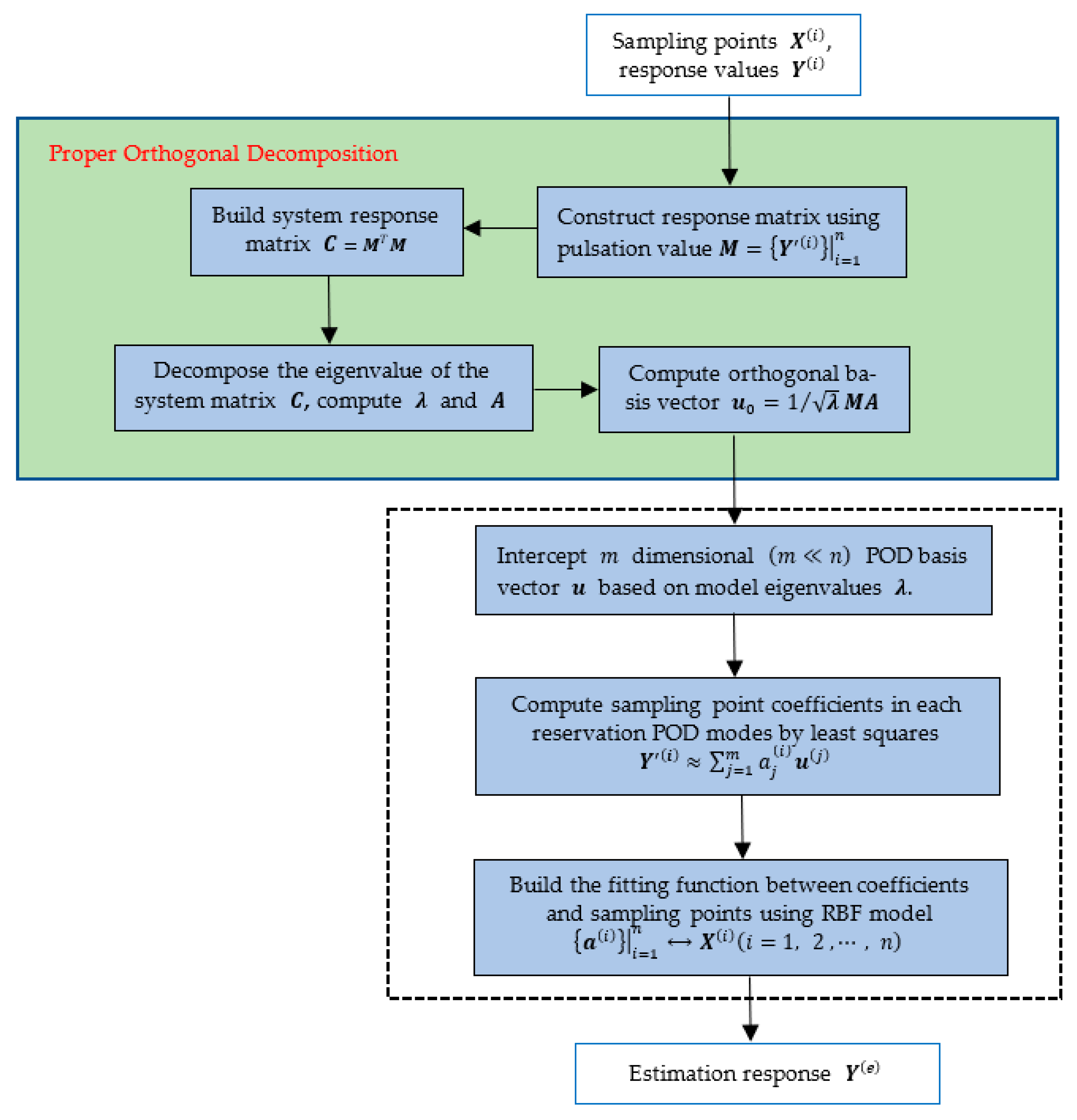
2. Rapid Data-Driven Prediction Method
2.1. Proper Orthogonal Decomposition
2.2. Radial Basis Function Interpolation
2.3. Rapid Prediction Method Based on Data-Driven
3. Numerical Simulation
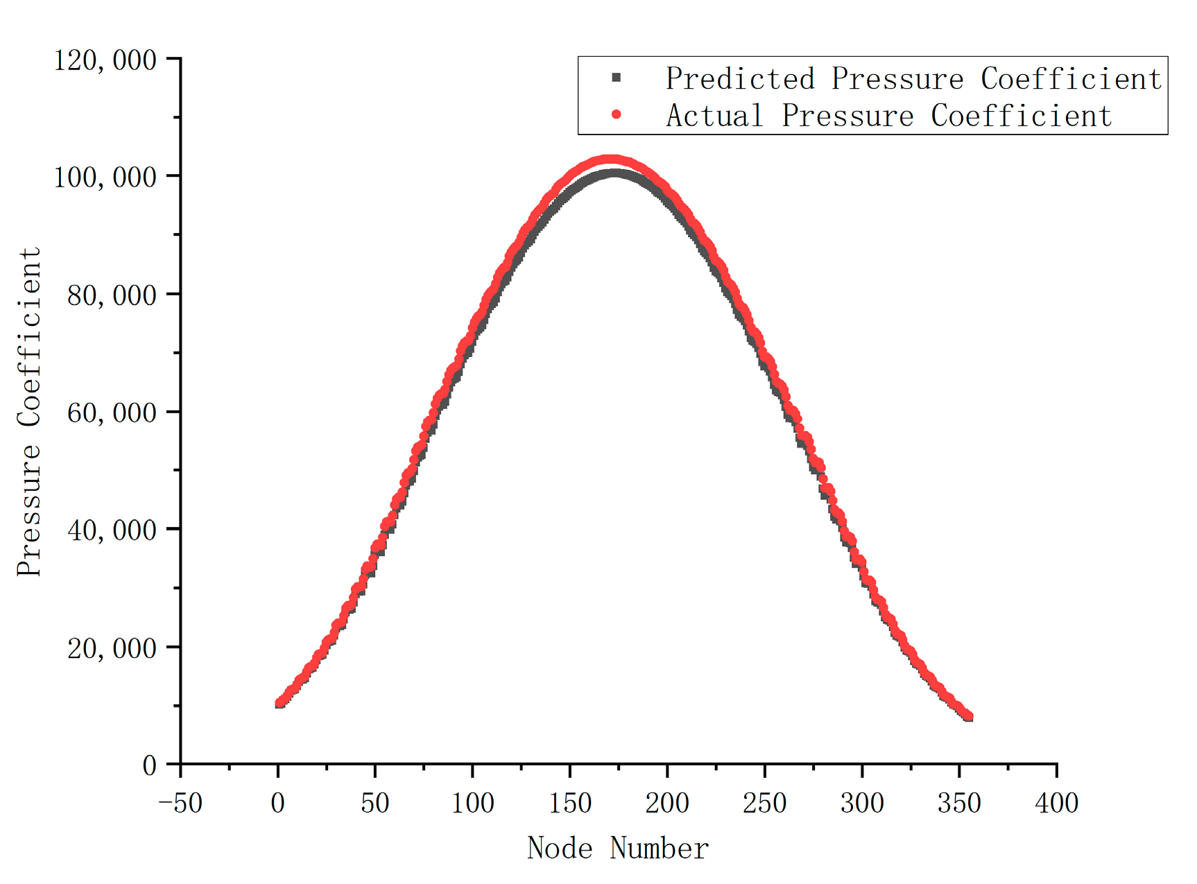
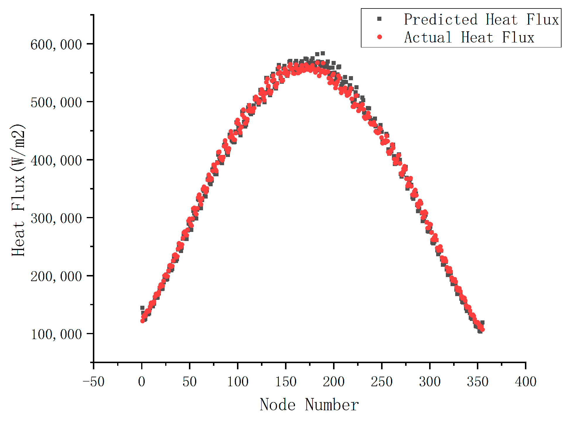
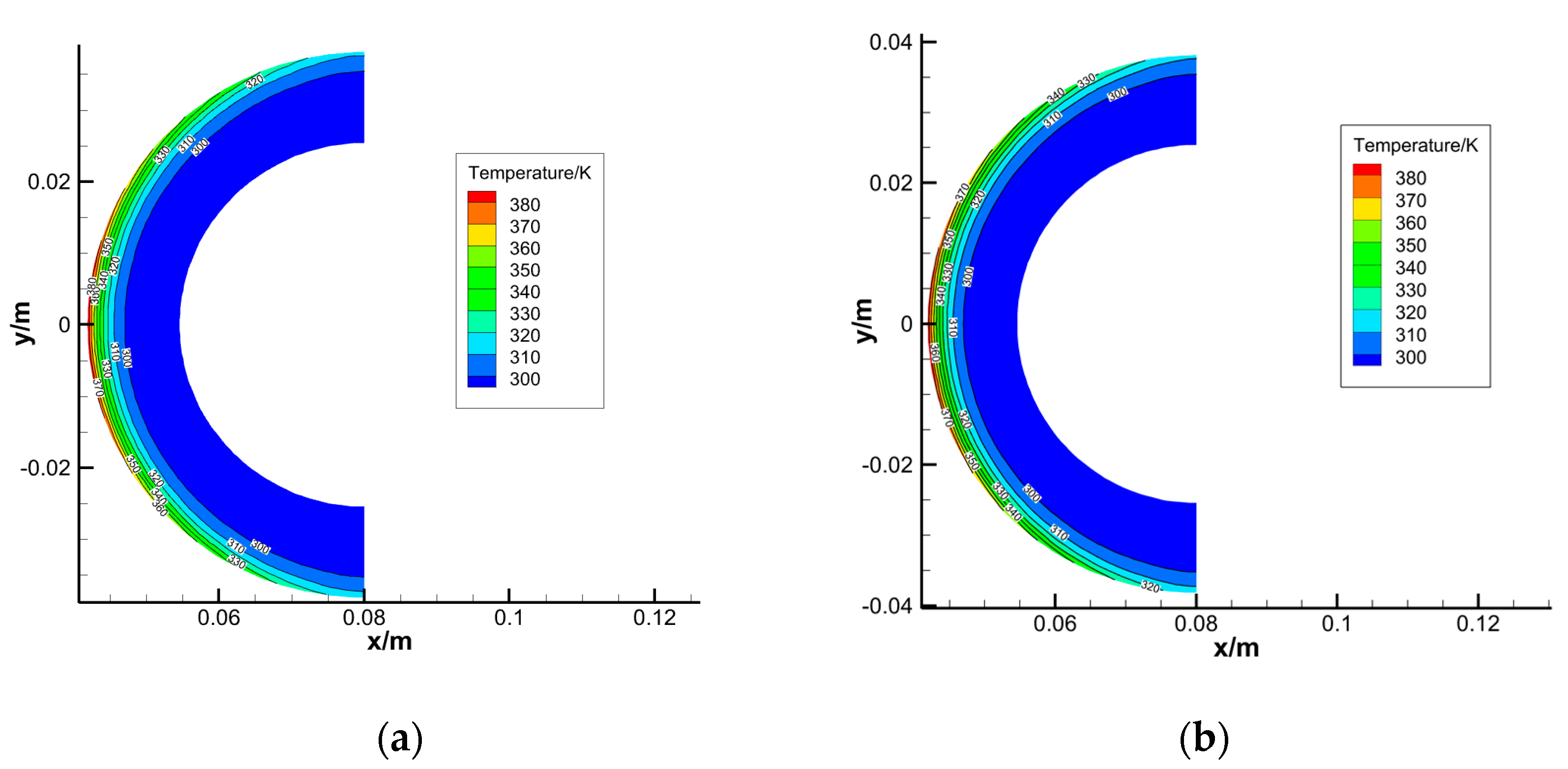
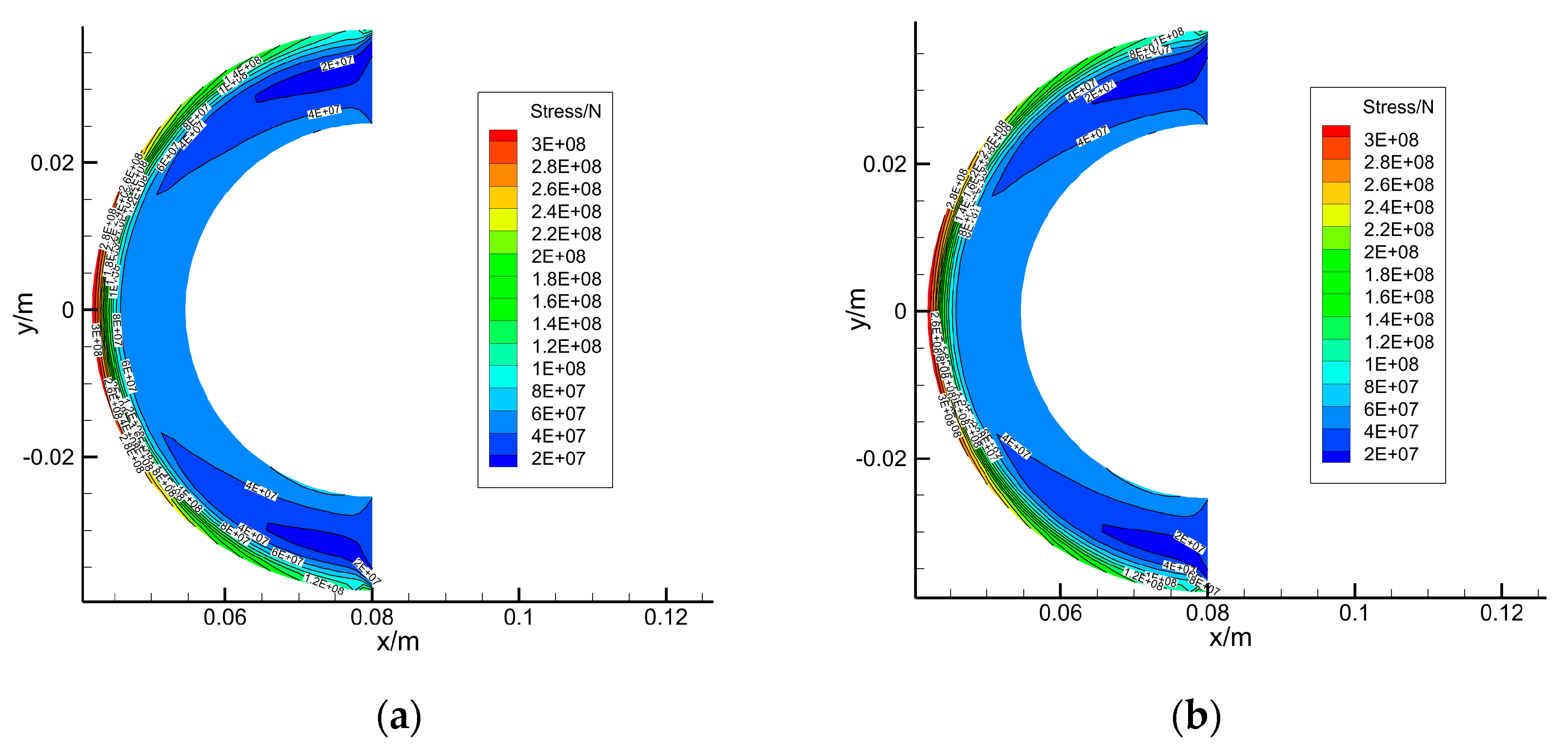
4. Result of Prediction
5. Conclusions
Author Contributions
Funding
Institutional Review Board Statement
Informed Consent Statement
Data Availability Statement
Conflicts of Interest
Appendix A

| Elastic Modulus | Poisson’s Ratio | Density | Coefficient of Linear Expansion | Thermal Conductivity | Specific Heat Capacity |
|---|---|---|---|---|---|
| 206 | 0.3 | 8030 | 17.5 | 16.27 | 502.48 |
References
- Zel’dovich, Y.B.; Raizer, Y.P. Elements of Gasdynamics and the Classical Theory of Shock Waves. In Physics of Shock Waves and High-Temperature Hydrodynamic Phenomena; Hayes, W.D., Probstein, R.F., Eds.; Dover Publications: Mineola, NY, USA, 1967; pp. 1–104. [Google Scholar]
- Hirschel, E.H. The Flight Environment. In Basics of Aerothermodynamics; Springer: Berlin, Germany, 2005; pp. 15–26. [Google Scholar]
- Anderson, J.D. Hypersonic Shock and Expansion-Wave Relations. In Hypersonic and High-Temperature Gas Dynamic; AIAA Press: Palo Alto, CA, USA, 2019; pp. 39–53. [Google Scholar]
- Shang, J.S.; Surzhikov, S.T. Radiative Energy Transfer. In Plasma Dynamics for Aerospace Engineering; Cambridge University Press: New York, NY, USA, 2018; pp. 304–336. [Google Scholar]
- Gui, Y.; Yuan, X. Numerical simulation on the coupling phenomena of aerodynamic heating with thermal response in the region of the leading edge. J. Eng. Thermophys. 2002, 23, 733–735. [Google Scholar]
- Chen, F.; Liu, H.; Zhang, S. Time-adaptive loosely coupled analysis on fluid–thermal–structural behaviors of hypersonic wing structures under sustained aeroheating. Aerosp. Sci. Technol. 2018, 78, 620–636. [Google Scholar] [CrossRef]
- Geng, X.; Liu, L.; Gui, Y.; Tang, W.; Wang, A. Studying the Temperature Field of Hypersonic Vehicle Structure with Aero-Thermo-Elasticity Deformation. Int. Sch. Sci. Res. Innov. 2015, 9, 1434–1437. [Google Scholar]
- Zhao, X.; Sun, Z.; Tang, L.; Zheng, G. Coupled flow-thermal-structural analysis of hypersonic aerodynamically heated cylindrical Leading Edge. Eng. Appl. Comput. Fluid Mech. 2011, 5, 170–179. [Google Scholar] [CrossRef] [Green Version]
- Korkegi, R.H. Survey of Viscous Interactions Associated with High Mach Number Flight. AIAA J. 1971, 9, 771–784. [Google Scholar] [CrossRef]
- Wieting, A.R. Experimental Study of Shock Wave Interference Heating on a Cylindrical Leading Edge. Ph.D. Thesis, Old Dominion University, Norfolk, VA, USA, 1987. [Google Scholar]
- Thornton, E.A.; Dechaumphai, P. Coupled Flow, Thermal and Structural Analysis of Aerodynamically heated Panels. J. Aircr. 1988, 25, 1052–1059. [Google Scholar] [CrossRef]
- Dechaumphai, P.; Thornton, E.A.; Wieting, A.R. Flow-Thermal-Structural Study of Aerodynamic Heated Leading Edges. J. Aircr. 1989, 26, 201–209. [Google Scholar]
- Li, J.; Wang, J.; Yang, L.; Shu, C. A hybrid lattice Boltzmann flux solver for integrated hypersonic fluid-thermal-structural analysis. Chin. J. Aeronaut. 2020, 33, 2295–2312. [Google Scholar] [CrossRef]
- Liu, H.; Wang, Z. Fluid–thermal–structural coupling investigations of opposing jet in hypersonic flows. Int. Commun. Heat Mass Transf. 2021, 120, 105017. [Google Scholar]
- Sirovich, L. Turbulence and the dynamics of coherent structures. Part 1: Coherent structures. Quart. Appl. Math. 1987, 45, 561–571. [Google Scholar] [CrossRef] [Green Version]
- Duan, Y.; Cai, J.; Li, Y. Gappy proper orthogonal decomposition-based two-step optimization for airfoil design. AIAA J. 2012, 50, 968–971. [Google Scholar] [CrossRef]
- Tan, B.; Damodaran, M.; Willcox, K. Aerodynamic data reconstruction and inverse design using proper orthogonal decomposition. AIAA J. 2004, 42, 1505–1516. [Google Scholar]
- Marc, O.; Markus, B.; Kilian, O.; Sonja, S. Statistical characterization of horizontal slug flow using snapshot proper orthogonal decomposition. Int. J. Multiph. Flow 2021, 134, 103453. [Google Scholar]
- Huang, D.; Jan, N.; Christian, W.; Peter, W. A machine learning based plasticity model using proper orthogonal decomposition. Comput. Methods Appl. Mech. Eng. 2020, 365, 113008. [Google Scholar] [CrossRef] [Green Version]
- Legresley, P.; Alonso, J. Airfoil design optimization using reduced order models based on proper orthogonal decomposition. Proc. AIAA Space 2000, 40, 1954–1960. [Google Scholar]
- Esmaeilbeigi, M.; Garmanjani, G. Gaussian radial basis function interpolant for the different data sites and basis centers. Calcolo 2017, 54, 155–166. [Google Scholar] [CrossRef]
- Wang, X.D.; Ding, Y.H.; Shao, H.H. The improved radial basis function neural network and its application. Artif. Life Robot. 1998, 2, 8–11. [Google Scholar] [CrossRef]
- Tyshchenko, O. A reservoir radial-basis function neural network in prediction tasks. Autom. Control Comput. Sci. 2016, 50, 65–71. [Google Scholar] [CrossRef]
- Cheng, Q.S.; Wu, L.W.; Wang, S.Z. Fusion prediction based on the attribute clustering network and the radial basis function. Chin. Sci. Bull. 2001, 46, 789–792. [Google Scholar] [CrossRef]
- Liu, Z.; Ning, F.; Zhai, Q.; Ding, H.; Wei, J. Study on the flow characteristics in the supersonic morphing cavities using direct numerical simulation and proper orthogonal decomposition. Wave Motion 2021, 104, 102751. [Google Scholar] [CrossRef]
- Di, G.; Dakun, S.; Ruize, X.; Daniel, B.; Sun, X.F.; Ni, S.L.; Du, J.; Zhao, D. Experimental investigation on axial compressor stall phenomena using aeroacoustics measurements via empirical mode and proper orthogonal decomposition methods. Aerosp. Sci. Technol. 2021, 112, 106655. [Google Scholar]
- Lukas, K.; Cyrille, V.; Christian, B. Using a Proper Orthogonal Decomposition representation of the aerodynamic forces for stochastic buffeting prediction. J. Fluids Struct. 2020, 99, 103178. [Google Scholar]
- Chen, X.; Liu, L.; Yue, Z. Reduced order aerothermodynamic modeling research for hypersonic vehicles based on proper orthogonal decomposition and surrogate method. Acta Aeronaut. Astronaut. Sin. 2015, 36, 462–472. [Google Scholar]
- Kou, J.; Zhang, W. Dynamic mode decomposition and its applications in fluid dynamics. Acta Aerodyn. Sin. 2018, 36, 163–179. [Google Scholar]
- Wang, Y.; Han, R.; Liu, Z. Progress of deep learning modeling technology for fluid mechanics. Acta Aeronaut. Astronaut. Sin. 2021, 42, 524779. [Google Scholar]
- Cui, E. MEMS and Intelligent Fluid Mechanics. Acta Aerodyn. Sin. 2000, 18, 52–59. [Google Scholar]
- Karami, S.; Soria, J. Analysis of Coherent Structures in an Under-Expanded Supersonic Impinging Jet Using Spectral Proper Orthogonal Decomposition (SPOD). Aerospace 2018, 5, 73. [Google Scholar] [CrossRef] [Green Version]
- Hu, Z. Research on Intelligent Prediction and Machine Learning Based on Big Data. Digit. Technol. Appl. 2021, 39, 84–86. [Google Scholar]
- Ren, F.; Gao, C.; Tang, H. Machine learning for flow control: Applications and development trends. Acta Aerodyn. Sin. 2021, 42, 524686. [Google Scholar]
- Lin, Y.; Guan, Z. The Use of Machine Learning for the Prediction of the Uniformity of the Degree of Cure of a Composite in an Autoclave. Aerospace 2021, 8, 130. [Google Scholar] [CrossRef]
- Hashemi, S.; Botez, R.; Grigorie, T. New Reliability Studies of Data-Driven Aircraft Trajectory Prediction. Aerospace 2020, 7, 145. [Google Scholar] [CrossRef]
- Uzun, M.; Demirezen, M.; Inalhan, G. Physics Guided Deep Learning for Data-Driven Aircraft Fuel Consumption Modeling. Aerospace 2021, 8, 44. [Google Scholar] [CrossRef]
- Lerro, A.; Brandl, A.; Battipede, M.; Gili, P. A Data-Driven Approach to Identify Flight Test Data Suitable to Design Angle of Attack Synthetic Sensor for Flight Control Systems. Aerospace 2020, 7, 63. [Google Scholar] [CrossRef]


| Method | Maximum Temperature of Structure/K | Maximum Pressure of Flow Field/Pa | |
|---|---|---|---|
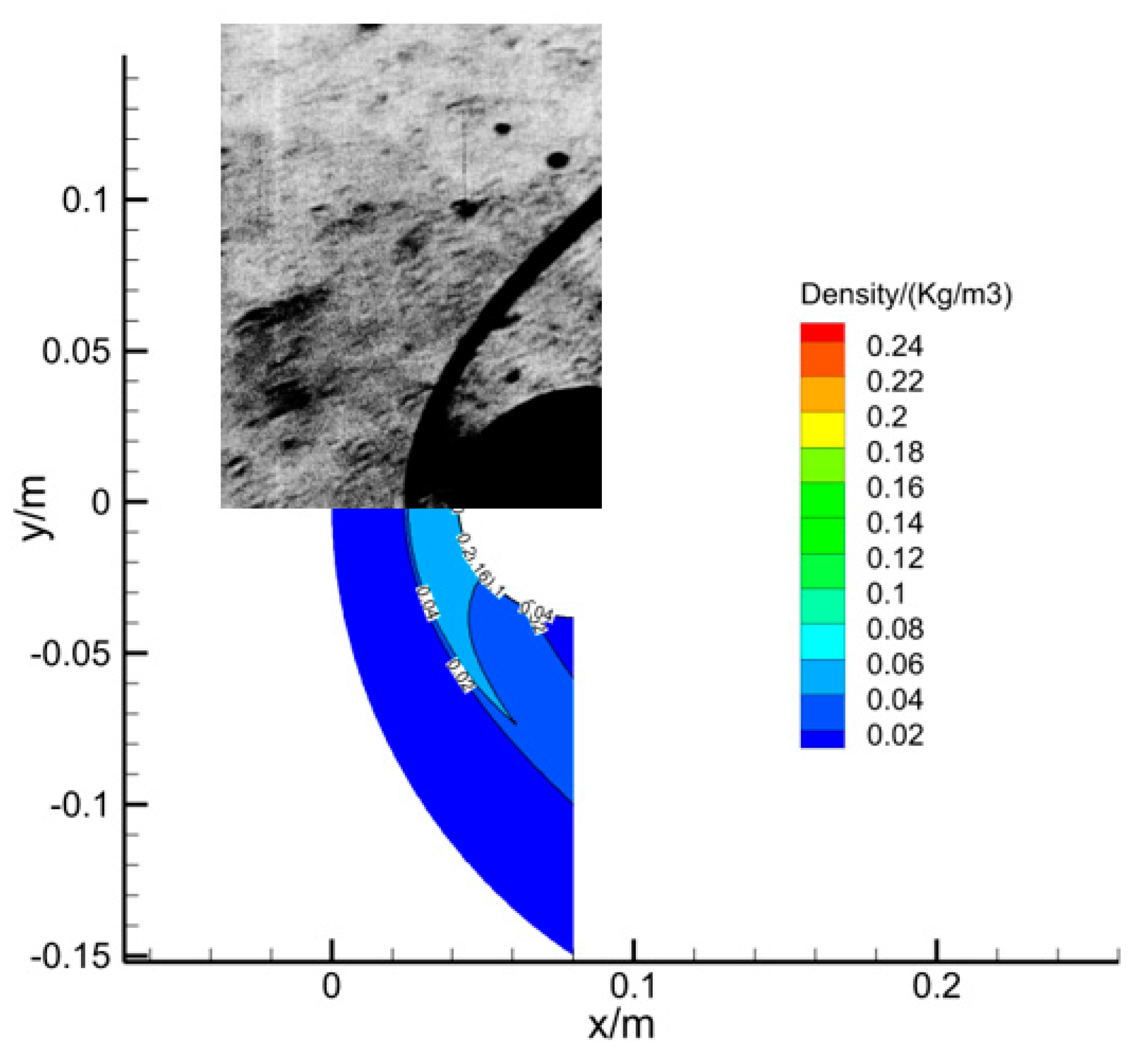
| Numerical Simulation in this paper | 436 | 663 | 35,386 |
| Experiment [10] | 465 | 670 | 37,815 |
| Test Condition | |||
|---|---|---|---|
| 1 | 38 | 4.2 | −3.2 |
| 2 | 26 | 5 | −6.4 |
| 3 | 30 | 3.4 | 3.2 |
| 4 | 34 | 6.6 | 0 |
| 5 | 22 | 5.8 | 6.4 |
| Method | Number of Snapshots | CPU Time for One Snapshot/h | CPU Time for Predicting one Test Condition/s |
|---|---|---|---|
| Prediction method | 5 | 0.14 | |
| Numerical simulation | 60 |
Publisher’s Note: MDPI stays neutral with regard to jurisdictional claims in published maps and institutional affiliations. |
© 2021 by the authors. Licensee MDPI, Basel, Switzerland. This article is an open access article distributed under the terms and conditions of the Creative Commons Attribution (CC BY) license (https://creativecommons.org/licenses/by/4.0/).
Share and Cite
Liu, J.; Wang, M.; Li, S. The Rapid Data-Driven Prediction Method of Coupled Fluid–Thermal–Structure for Hypersonic Vehicles. Aerospace 2021, 8, 265. https://doi.org/10.3390/aerospace8090265
Liu J, Wang M, Li S. The Rapid Data-Driven Prediction Method of Coupled Fluid–Thermal–Structure for Hypersonic Vehicles. Aerospace. 2021; 8(9):265. https://doi.org/10.3390/aerospace8090265
Chicago/Turabian StyleLiu, Jing, Meng Wang, and Shu Li. 2021. "The Rapid Data-Driven Prediction Method of Coupled Fluid–Thermal–Structure for Hypersonic Vehicles" Aerospace 8, no. 9: 265. https://doi.org/10.3390/aerospace8090265