Article

Prediction of Aircraft Noise Impact with Application to Hong Kong International Airport

School of Mechanical & Aerospace Engineering, The Hong Kong University of Science & Technology, Hong Kong, China
*
Author to whom correspondence should be addressed.
Aerospace 2021, 8(9), 264; https://doi.org/10.3390/aerospace8090264
Submission received: 6 August 2021 / Revised: 9 September 2021 / Accepted: 10 September 2021 / Published: 15 September 2021
(This article belongs to the Special Issue Aircraft Noise)

Abstract

:
As part of a collective research effort towards greener aviation, the present study focuses on the noise impact of aircraft operations around major airports. To this end, an aircraft noise prediction platform is developed, which relies on state-of-the-art functionalities as well as more specific, innovative features. Originally built upon the Aircraft Noise and Performance (ANP) database and its Noise–Power–Distance (NPD) table, the method is further refined to alleviate most of their inherent limitations (e.g., standardized and simplified aircraft noise scenarios). The resulting aircraft noise prediction platform is validated against benchmark cases of increasing complexity, being then applied to real-life situations involving actual aircraft operations around Hong Kong International Airport (HKIA). Specific comparative analyses are conducted, which allow highlighting the variability of the noise impact by aircraft, depending on their type (A330, B777) and/or operational conditions (power settings, meteorological conditions, routes, banks, etc.). The study delivers insightful outcomes, whether phenomenological (aircraft noise impact) or methodological (aircraft noise prediction). As a by-product, it illustrates how noise prediction methods/platforms such as the present one may help in guiding the further expansion of airport operations and/or infrastructures (as is currently the case with HKIA).

1. Introduction

The development of low-noise technologies and the establishment of more stringent regulations have led to a continuous decrease in the noise impact by air traffic over recent decades [1]. However, the environmental noise pollution caused by civil aviation is still a major societal concern, because of the many adverse effects it entails (annoyances, sleep disturbances, health issues, educational achievements, etc.) [2,3,4]. This makes aircraft noise a show-stopper for airports expansion [5], which may question the sustainable development of the aviation market [6,7,8] whose annual growth is about 5% [9]. Therefore, mitigating the noise impact of civil aviation is of utmost importance for all major countries, especially those which possess large aviation hubs located nearby highly dense cities, such as China [10,11]. Indeed, not only China is the most populous country in the world, but it also ranks second in the world in terms of passenger air traffic and it has now replaced the United States as the world’s largest aviation market [12]. In particular, Hong Kong, which is the world’s sixth most densely populated city, is also the busiest airport in terms of cargo volume, worldwide. To cope with the growing demand for air transportation, the Hong Kong International Airport (HKIA) is now expanding its capacity, through the deployment of a third runway [13]. This obviously raises legitimate concerns about how the noise impact by aircraft operations will affect the many residential areas surrounding HKIA.
Aircraft noise has been a matter of intense research over the past 50 years. Essentially, two main approaches exist to mitigate aircraft noise, namely at the aircraft level by reducing its sources [14] and at the operation level by reducing its perceived impact on the ground [15,16,17]. The former strategy seeks at developing quieter engines and low-noise aircraft designs [18], which however constitutes a daunting challenge given the multiple components involved (e.g., high-speed jets, combustion, turbine, fan, landing gear, high-lift devices, cavities, etc.) [19,20]. The latter strategy rather seeks at optimizing the aircraft operations nearby airports (e.g., through noise abatement flight procedures) [17,21,22]. This however requires properly assessing the noise impact induced by aircraft during their departure and approach flight phases, which can be achieved through field measurements and/or predictive models. Field measurements are relatively straightforward and reliable [23], but they can only be performed a posteriori, over certain predetermined locations (e.g., using in-situ microphones). Notably, they solely offer measuring the noise impact from actual aircraft operations, but they do not allow to extrapolate it to alternative scenarios (e.g., for exploring the impact of new flightpaths, runways, fleets, noise abatement procedures, etc.). Moreover, field measurements can be polluted by ambient sounds, which makes it more difficult to discriminate the actual aircraft noise [24]. All these issues can be overcome by using predictive models, whose principle is to virtually recreate the noise impact by aircraft operations. The major limitation of these models is their cost in terms of computational resources, which scale with the accuracy level that is sought after. Over recent decades, many aircraft noise prediction approaches were proposed, which can be subdivided into three categories [25,26], namely, empirical [27,28,29,30], semi-empirical [31,32,33] and analytical [34,35,36]. Falling in the first category, the so-called Integrated Noise Model (INM) [37] developed by the US Federal Aviation Administration (FAA) is used worldwide for assessing the noise impact around airports. This tool is commonly used for either (i) monitoring aircraft operations, (ii) studying their impact on the neighboring populations [38,39,40], (iii) guiding the further development of airports [22,41,42], or even (iv) establishing low-noise flight procedures [43,44]—all that whereas incorporating other constraints (e.g., fuel consumption and chemical emissions) [45,46]. In particular, the INM model is now the cornerstone of large prediction platforms aiming at optimizing airport operations, worldwide, such as the Aviation Environmental Design Tool (AEDT) in the U.S.A. The latter constitutes one of the major bricks of the FAA-led Next Generation Air Transport System [47], whose goal is to revamp America’s aviation infrastructures and operations into a renewed, integrated, clean and efficient air system [47]. Similar large-scale initiatives exist worldwide, for instance in Europe with the Environmental Noise Directive [48], whose aircraft noise aspects are tackled using methods that also rely on the INM model. Notably, the baseline methodology underlying INM is best described in ref [49], which was issued by a concertation group of the European Civil Aviation Conference (ECAC) in the framework of the END initiative [48]. Since the latter initiative extends to other industries (civilian and military aviation, railway, road traffic, etc.), current efforts focus on unifying and standardizing the prediction tools for environmental noise mitigation, for instance by developing the so-called Common Noise Assessment Methods in Europe [50]. Regarding aviation noise, the CNOSSOS-EU approach also relies on the INM model whereas integrating additional databases, thereby offering to tackle not only civilian aircraft, but also military ones, as well as helicopters, or specific airport operations (e.g., engine run-up noise). This may be pivotal in implementing strategic noise maps [51,52], thereby helping policymakers in their efforts to improve the land-use planning around major airports, as advocated by ICAO for mitigating environmental noise by air traffic. All the above illustrates how aircraft noise prediction tools can be advantageously integrated into larger platforms, thereby allowing to tackle environmental issues that would be too challenging to handle otherwise.
The present study is part of a larger research effort, whose objective is to develop a flightpath optimization platform enabling to minimize both the fuel consumption and noise emission due to aircraft operations nearby airports [45]. As a starting point, we here develop a noise prediction approach that comes as a mix between the INM baseline methodology [49] and novel, specific features. Upon incremental validations, we apply the resulting approach/tool to actual aircraft operations, thereby highlighting its relevance for real-life situations. This paper is organized as follows. In Section 2, the noise prediction approach is outlined, with a special emphasis put on the specific improvements that were brought to it. The method and subsequent tool are then validated in Section 3, this being achieved using several benchmark cases of increasing representativeness. In Section 4, the approach is applied to realistic scenarios coming from actual aircraft operations nearby Hong Kong International Airport. Finally, some conclusions and perspectives are drawn.

2. Computational Methodology
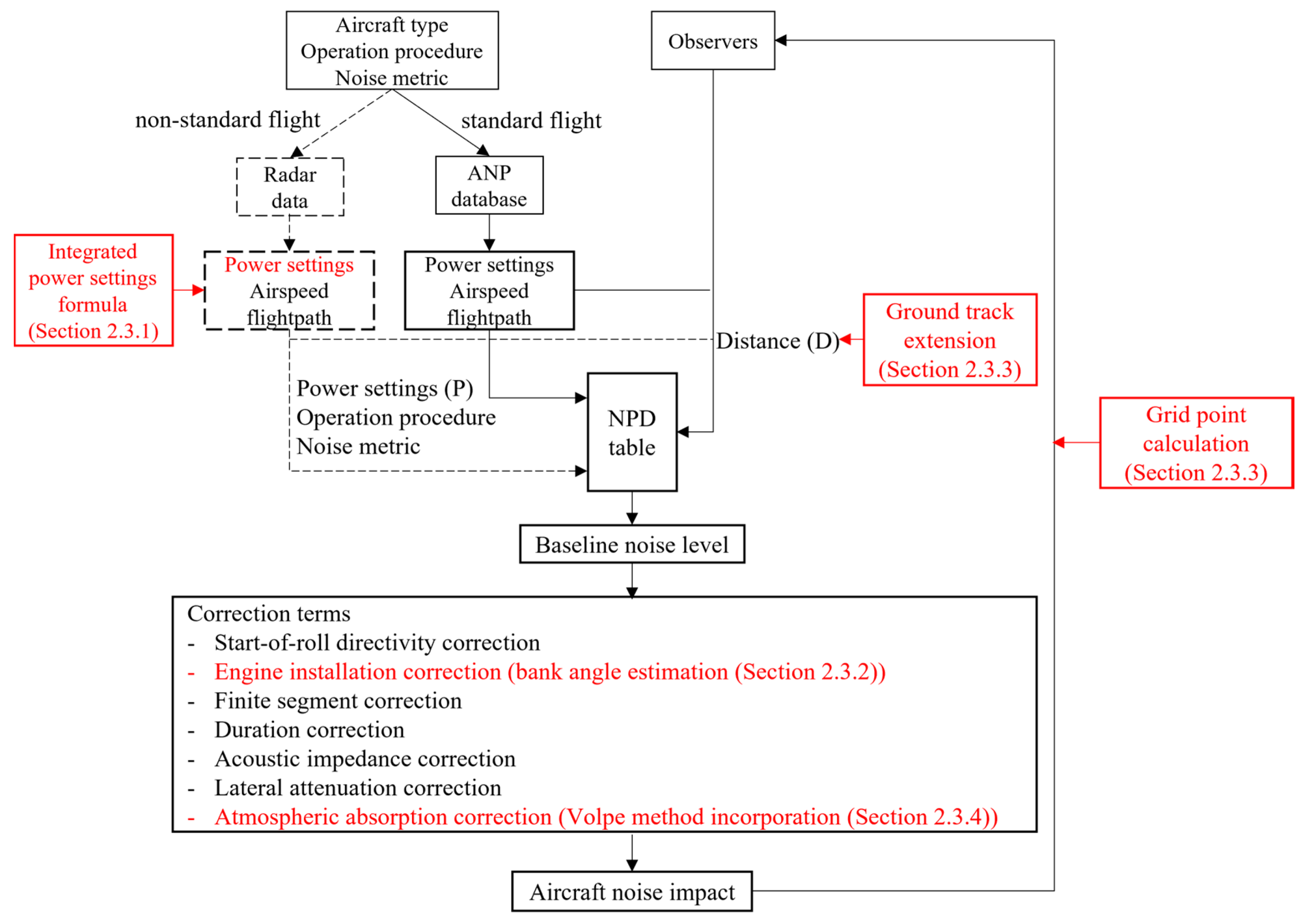
This section outlines the present noise prediction approach, which incorporates specific supplements compared to the baseline methodology described in [49].

2.1. Overview

Similar to the INM-related baseline methodology it originates from, the present approach primarily relies on the so-called Aircraft Noise and Performance (ANP) database and its associated Noise–Power–Distance (NPD) subset. This ANP/NPD database can be seen as a semi-empirical tool that allows estimating the noise impact induced by a given aircraft, depending on what its power settings and distance to the ground are [53]. Here it is worth reminding that such a noise impact is commonly measured in terms of Sound Exposure Level (SEL) or Effective Perceived Noise Level (EPNL), both of which represent the overall sound energy of a single noise event once integrated over a given duration (one and ten seconds, respectively) [37,54] and tailored to the sensitivity of the human ear (e.g., the SEL is A-weighted and the EPNL is tone corrected). Both measures thus translate the loudness or noisiness of the noise event, whereas their cumulative effect over successive events can be averaged (e.g., Day–Night average sound Level, DNL, Equivalent Sound Level, Leq). Given its empirical nature, the ANP/NPD database/tool is a powerful resource for predicting the noise environment around airports. On the other hand, since it is built upon standardized scenarios of aircraft operations (aircraft types, flightpaths, power settings, atmospheric conditions, etc.), its application is limited to rather canonical situations of air transport exploitation. Moreover, since the NPD-based noise prediction kernel relies on a rather rudimentary scenario of noise emission by a simplistic source (isolated jet) within a homogeneous free-field medium, the approach somehow lacks accuracy. One way to mitigate these limitations is to improve both the source characteristics and the propagation features that the approach relies on, which can be partly achieved by incorporating additional correction factors. This is what was carried out here and is summarized below.
On one hand, the characteristics of the noise source can be improved through a more accurate description of both its intensity and directivity. First, the source intensity is directly driven by the aircraft power settings, which can be refined by using the actual ones instead of their standardized counterparts. To this end, Section 2.3.1 proposes a method for assessing the actual power settings of an aircraft, based on its flightpath characteristics. Second, the source directivity is related to the way the engines are installed within the airframe (e.g., wing-mounted or fuselage-mounted), with an installation effect that can be partly incorporated through the proper estimation of the aircraft bank angle (see Section 2.3.2). On the other hand, the propagation features can be refined through several means such as a more accurate description of the propagative path itself (e.g., incorporating all the flightpath sections that contribute to the noise impact, see Section 2.3.3), as well as of the noise phenomena to occur during the propagation phase (e.g., absorption due to the humidity, refraction due to the atmosphere inhomogeneities, reflection due to the ground, etc.). Some of these refinements are part of the INM-based method which is described in Section 2.2, whereas others are specific to the current work and are detailed in Section 2.3. Yet, not all of these effects can be incorporated in the approach, which would be too complex and costly otherwise. For instance, one can here remind that the sound refraction originates from the atmospheric heterogeneities, which either affect the sound speed (and thus the acoustic impedance) through the pressure and temperature variations, or add convection effects due to winds. Whereas the former effect can be incorporated in a rather straightforward manner, the latter raises more challenges in terms of practical implementations and CPU cost efficiency.
Figure 1 sketches the overall methodology, both summarizing the baseline approach [49] and highlighting the specific addendums brought to it in the present work.

2.2. Baseline Approach

This section gives a brief overview of the baseline approach, whose detail can be found in [49]. Recommended by the International Civil Aviation Organization (ICAO), this approach is widely adopted by airports and legislation authorities for assessing the noise impact of aircraft operations (at least for commercial aircraft) [55].
As detailed in ref [53], this methodology relies on the fragmentation of the flightpath into specific segments, each one being allotted the aircraft corresponding characteristics (position, power settings, airspeed, etc.). Those characteristics are then translated into suitable inputs (power settings, aircraft-to-ground distance) for the NPD-based noise prediction tool to assess the aircraft noise impact on the ground. More precisely, the 3D flightpath is decomposed into the so-called ground track (i.e., the vertical projection of the flightpath on the ground) and flight profile (i.e., the altitude changes of the aircraft along the ground track), both of which are made of a finite number of continuous straight-line segments. The detail of these flight segments (endpoints) and associated aircraft characteristics (operational data) can be inferred from the flightpath records (either radar or Flight Data Recorder, FDR), or estimated using specific formulas [49]. Using this, the aircraft power settings and aircraft-to-ground distance can be obtained, thereby allowing the aircraft noise impact to be assessed through proper (linear and logarithmic) interpolations of the NPD database.
As was said, however, the NPD database is built upon an ideal scenario following which the ground observer would be located right below the aircraft, with the latter flying at a constant speed and power settings along an infinite horizontal flightpath and under specific atmospheric conditions. For the method can be applied to more realistic scenarios, it is thus needed to enhance it with several correction terms, namely, start-of-roll directivity, engine installation, finite segment, duration, acoustic impedance, and lateral attenuation adjustments. The start-of-roll directivity correction reflects the highly directive radiation pattern of the engine noise during the take-off roll. The engine installation correction accounts for the modification of the aircraft noise source directivity due to the integration of the engines within the airframe (e.g., scattering by the wings, refraction effects in the near-field, etc.). The finite segment correction translates the fact that, different from the NPD assumption, the flightpath is made of finite segments. The duration correction accounts for the difference between the actual aircraft speed and that from the NPD standard (160 knots), such disparity in speed translating into shorter or longer sound exposures. The acoustic impedance adjustment accounts for the difference between the local atmospheric conditions (taken at the airport level [49]) and that from the NPD standard. The lateral attenuation translates all the noise interferences induced by the reflection (and, to a lesser extent, by the refraction) effects inherited from the ground presence. Here it is worth noticing that these refraction effects are incurred by either the temperature and/or wind gradients induced by the ground, depending on its characteristics (e.g., roughness, heat transfer). All these correction terms enable the NPD-based noise prediction tool to assess more accurately the noise impact of aircraft in different scenarios. As an illustration, Appendix B exemplifies how these various correction terms weigh on the prediction of the noise impact by a typical aircraft at take-off.

2.3. Specific Improvements Brought to the Methodology

The ANP database is built on a standardized scenario of aircraft operations (flight profile, power settings, airspeed, etc.). However, in reality, the actual operations often deviate from these standard cases, due to various factors (terrain, wind speed and direction, noise abatement flight procedure, etc.). For the overall methodology to be closer to reality, the NPD-based noise prediction must therefore be enhanced with various refinements—which was carried out here and is summarized hereafter.

2.3.1. Refinement of the Aircraft Noise Emission (Intensity), through the Incorporation of the Actual Power Settings

Ideally, the aircraft operational data should be inferred directly from actual records (either radar or Flight Data Recorder, FDR). Whereas FDR data offer the most comprehensive and accurate information, their proprietary nature makes them difficult to access. Conversely, radar data are open source and therefore readily available but they offer less detailed information. For instance, the flightpath characteristics of any aircraft can be easily accessed through their radar data, which can be accessed via public domain websites (e.g., FlightAware, Flightradar24, OpenSky Network, etc.). These data, however, do not provide any insights about the aircraft power settings, which makes them less straightforward to use in the present context. To overcome this issue, the present approach incorporates a functionality that offers assessing the aircraft power settings directly from the flightpath characteristics (flight profile and airspeed). To this end, we derive a simplified model for the thrust to be delivered by the engines when the aircraft is in dynamic equilibrium, whether it is considered at roll or aloft. By developing the corresponding equations of motion (cf. Appendix A), one can express the aircraft thrust via the following integrated formula (which is valid whether the flight segment is, i.e., either ground roll or aloft):
T = m [ a + g ( μ F c o s γ + μ F s i n γ ) ] + L [ C D C L + c o s ϕ · ( s i n γ μ F c o s γ c o s γ + μ F s i n γ ) ]
In the above, T indicates the thrust (in lbf), L is the lift force, C D / C L is the drag-to-lift ratio, m is the aircraft mass (in lbm), a is the aircraft inertial acceleration (in average), g is the gravitational acceleration. Besides, γ and ϕ , respectively, stand for the flightpath and bank angles (which are zero when the aircraft is on its ground roll). On the other hand, μ F is the friction coefficient [56], which accounts for the additional drag effect due to the runway (and is zero when the aircraft is aloft). From there, two scenarios can be distinguished:
When the aircraft is aloft ( μ F = 0 ), Equation (1) can be re-expressed as (cf. Appendix A)
T = m [ a + g ( C D C L · c o s γ cos ϕ + s i n γ ) ]
Oppositely, when the aircraft is on the ground roll ( γ = ϕ = 0 ), and by introducing a lift model [57], one can show that (cf. Appendix A)
T = m { a + g [ C D C L · ( V T A S V L O F ) 2 + μ F ( 1 ( V T A S V L O F ) 2 ) ] }
where V T A S and V L O F stand for the aircraft true airspeed (TAS) and its value at lift-off, respectively.
All parameters appearing in the above Equations (2) and (3) are readily available from the flight data and/or ANP database, for each aircraft type and flight setting. One can thus get the actual thrust directly from the aircraft and flight parameters, in all flight phases (whether the aircraft is aloft or on its ground roll). For being readily exploitable, however, the actual thrust must be scaled back to the standardized value upon which the NPD database is built upon, namely the corrected net thrust at sea level. To do so, the actual thrust is then adjusted through a gross-to-net thrust factor, which translates the fact that the thrust delivered at a given altitude deviates from its sea-level counterpart. This factor can be expressed through δ , the ratio of the ambient air pressure around the aircraft to the standard air pressure at mean sea level [23]. Once scaled by the number of engines, N, one finally gets the corrected net thrust per engine, to be used as input for the NPD database.
F n = T N δ

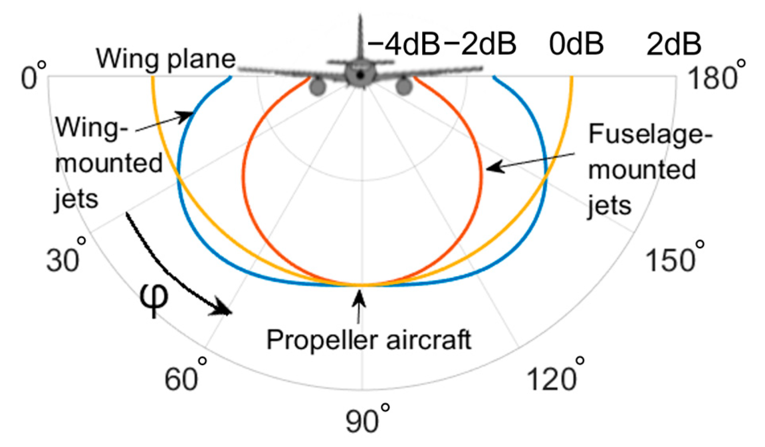
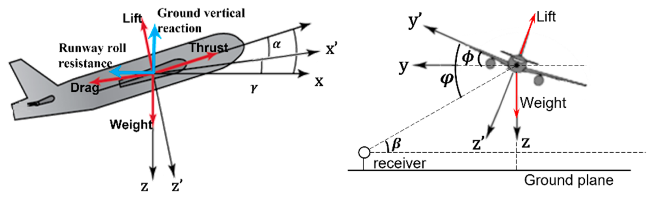
2.3.2. Refinement of the Aircraft Noise Emission (Directivity), through the Incorporation of the Engine Installation Effects (Bank Angle)

The way the engines are mounted within the airframe affects the directivity of the aircraft noise source. These so-called acoustic installation effects can be partially incorporated through the aircraft bank angle [49], which relates to the depression angle ( φ ) that is directly linked to the engine installation (see Figure 2 below, as well as Figure A1 in Appendix A). Indeed, when installed on an aircraft, engines see their noise directivity importantly altered because of the multiple scattering effects induced by the airframe elements (e.g., wings) [23]. This directivity, which is measured through the depression angle, mostly depends on the way the engines are positioned within the airframe (e.g., wing-mounted, fuselage-mounted). From a ground observer perspective, the noise intensity is thus to be driven by the combination of the depression and bank angles.
In the absence of any specific formulas provided in Ref [49], the aircraft bank angle is here estimated through the flightpath turn radius, using a geometrical approach [37]. To do so, the ground track is first approximated (using cubic spline interpolation) as a succession of evenly spaced points, each one being then inferred its corresponding turn radius (which is determined from the circumradius of the triangle formed with its two neighboring points). From there, using the aircraft airspeed along with the gravitational acceleration, the bank angle is derived [49]. Once filtered out from all possible irregularities coming from the flight characteristics inaccuracies (especially the aircraft position and airspeed), the bank angle values are interpolated back to the original ground track. Section 4.3.1 and Appendix C illustrate the sensitivity of the noise prediction towards these bank effects.

2.3.3. Refinement of the Aircraft Noise Propagation (Distance), through the Dynamic Specification of the Ground Track and Observers

Dynamic Extension on the Ground Track

By definition, the departure flight sequence begins when the aircraft initiates its ground roll and terminates once it has climbed up to an altitude of 10,000 ft. Oppositely, the approach flight sequence starts when the aircraft has descended down to an altitude of 6000 ft and finishes at the end of the landing ground-roll [37]. Because of this somehow arbitrary definition of the departure and approach procedures, any flightpath segment that would be beyond their altitude ranges is usually discarded in the aircraft noise assessment process. This may lead to underestimating the noise levels on the ground, whose discarded flight segments may still contribute to, depending on the situation (e.g., aircraft settings/flightpath ⇔ ground observer relationship). In order to correct such a potential bias in the noise estimation, some authors proposed to automatically enhance the default flight sequences with an extra flight segment, of arbitrary length [49]. Given its arbitrary nature, however, this fix may be partially conclusive (e.g., extra flight segment of insufficient length). Therefore, we here propose to rather incorporate all the flightpath segments that actually contribute to the noise impact on the ground, on a case-by-case basis. To do so, the flight sequence is extended in a dynamic fashion, being automatically added all the flight segments that are beyond its standard altitude range—this being carried out until their contribution to the aircraft noise impact is negligible, i.e., the noise levels on the ground are converged. More detail about this process is provided in Section 4.3.2.

Dynamic Specification of Ground Observers

Classically, the aircraft noise impact is characterized using a set of ground observer locations, over which the noise contribution by the various flight segments is summed up over time—all this leading to integrated noise contour maps. The overall efficiency (i.e., accuracy and rapidity) of the noise prediction is directly driven by the number and distribution of these prediction points. Therefore, past researches focused on how to optimize the latter, for instance using irregular grids [58,59]. Different from the baseline methodology, the present method incorporates an advanced dynamic grid refinement functionality [37], which allows increasing locally the density of observers wherever and whenever needed. This dynamic, local grid refinement process is conducted automatically during the noise prediction, which can be seen as a multi-stage calculation. More precisely, the noise prediction is first conducted on a coarse mesh, being then bi-linearly interpolated on a twice finer grid. The interpolated result is then compared to that of the direct calculation, which is repeated for each new grid point created. Whenever the two results fall within a certain threshold, the calculation is considered converged, and the local grid refinement stops. Should this not be the case, the process is repeated, until a local convergence is reached. Besides the tolerance (i.e., interpolation accuracy threshold), the degree of refinement is controlled through two other criteria, namely, the maximum refinement level allowed (with respect to the initial, coarse grid), and some pre-defined extrema of noise levels. Thanks to such a dynamic grid refinement functionality, the calculation process is optimal, offering the best trade-off in terms of accuracy and cost.

2.3.4. Refinement of the Aircraft Noise Propagation (Attenuation), through the Incorporation of Meteorological Effects

Aside from its emission characteristics (intensity, directivity), the aircraft noise is also driven by the properties of the atmospheric medium through which it propagates to the ground. It is not rare, however, that the actual atmospheric conditions deviate from the standard values upon which the NPD database is built. In this case, the noise prediction must be corrected from the specific biases induced by these offsets in atmospheric properties [55]. This can be achieved through two correction terms, namely, the acoustic impedance adjustment and the atmospheric absorption adjustment. The former correction accounts for the offset in the sound speed (which is driven by the atmospheric pressure and temperature values) whereas the latter accounts for the offset in the noise absorption effect (which is primarily driven by the temperature and relative humidity).

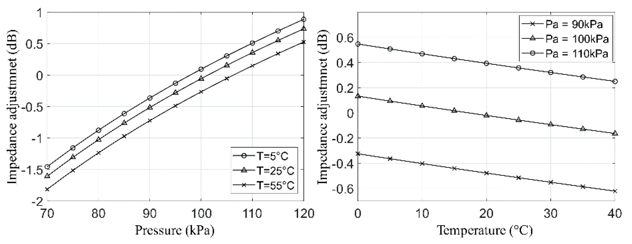
Deviation of the Sound Speed Characteristics (Acoustic Impedance Adjustment)

Acoustic impedance adjustment accounts for the deviation of the medium sound speed with respect to its NPD standard value. This correction term [49] is classically built as a function of the atmospheric pressure and temperature (e.g. using Equation (4–6) and Equation (4–7) from Ref. [49]), both of which have a monotonic effect on the propagation. As exemplified in Figure 3, a rise in pressure (resp. temperature) shall result in a higher (resp. lower) correction required. The latter corrections, however, are usually moderate, with a variability that remains in the order of a decibel (dB). For instance, a pressure increase of 50 kPa entails a difference of +2.3 dB (regardless of the temperature), whereas a temperature increase of 40 °C induces an effect of −0.3 dB, regardless of the pressure.

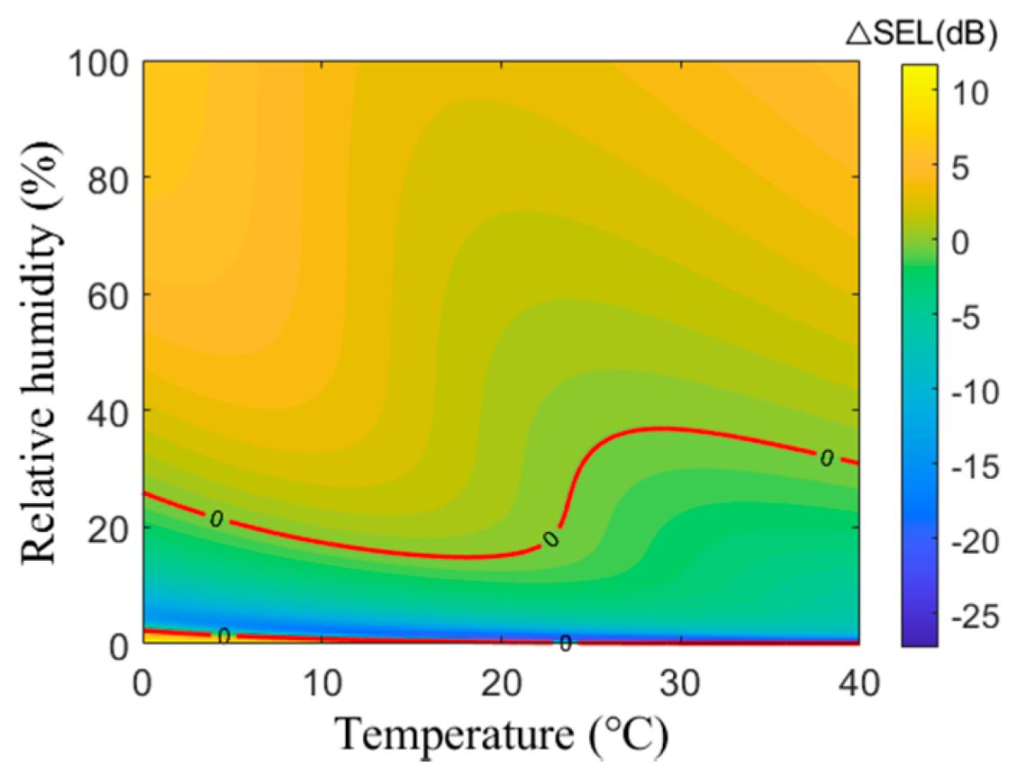
Deviation of the Sound Absorption Characteristics (Atmospheric Absorption Adjustment)

The atmospheric absorption relates to the energy dissipation that sound waves experience when interacting with air molecules. It is mostly driven by the temperature and relative humidity, upon which the atmospheric absorption adjustment is thus usually built [60]. As an illustration, Figure 4 depicts the difference in the noise levels that are radiated on the ground by a given sound source located at an altitude of 25,000 ft, depending on if the propagation medium corresponds to a standard or a non-standard atmosphere. As can be seen, these differences are nonlinear and non-monotonic, which makes it uneasy to predict how a given deviation in temperature and/or relative humidity shall impact the noise prediction. Notably, these effects may cancel out each other—as highlighted in Figure 4 by the red line, which depicts those atmospheric conditions for which the difference is nil. In the present approach, the atmospheric absorption adjustment not only incorporates the deviations in temperature and/or relative humidity (as classically carried out [60]), but it also includes those in atmospheric pressure. Relying on the so-called Volpe method [61], this correction is thus expected to yield still more accurate results, especially for what concerns long-distance propagation. For more detail about this correction term, the interested reader is referred to Ref. [49] (Equations (D-1) to (D-4)) and Ref. [61] (Equations (1) to (6), Equations (16) and (17)). These atmospheric absorption effects are further discussed in Section 4.2.

3. Validation of the Methodology Using Standardized Cases

In this section, the present noise prediction approach is validated using benchmark cases, which correspond to either virtual standard scenarios or to real-life but well-known situations (noise certification tests).

3.1. Standardized Scenarios

Here, we consider a total of 12 standardized scenarios, which were previously documented in [62]. These cases describe the noise impact induced by an aircraft, depending on its type and/or flightpath. More precisely, we here consider three different types of aircraft, namely, a jet-powered aircraft with either fuselage-mounted (JETF) or wing-mounted (JETW) engines, as well as a propeller-powered aircraft (PROP). Each aircraft is taken under either a departure (D) or an approach (A) flight, which both follow either a straight (S) or a curved (C) route. Please, see Ref. [62] for a detailed description of these benchmark cases, some aspects of which are nevertheless further documented in Appendix B (e.g., aircraft routes, observers locations).
Figure 5 and Figure 6, respectively, depict the noise contour maps associated with all three aircraft at departure and approach (only the curved routes are considered, for the sake of conciseness). Of note, the noise metric used here is Sound Exposure Level (SEL). For each case, the differences between the present prediction and the reference one [62] are quantified using error maps (obtained by subtracting the reference values from the calculated results). As one can see, the agreement is good, with absolute error levels that are typically less than 0.01 dB. Notably, compared to some of the past works [23], the present calculations rely on a coarser distribution of ground observers, whereas delivering more accurate results (compare for instance the error map of JETFDC case with its counterpart from Ref. [23] whose visual rendering was here duplicated on purpose.).
This good agreement is verified for all 12 benchmark cases, as shown in Table 1, which quantifies the mismatches between the present predictions and the reference values. For each case, this mismatch is characterized via both the maximum absolute error ( δ max ) and the average (root-mean-square) error δ RMS , as recorded throughout the ground observers. Notably, for all cases, the average error, δ RMS , is much less than the threshold of 0.01 dB, which is the indicator of a reliable prediction [62]. Moreover, this accuracy level appears to be higher than the one reached by previous similar studies which focused on the same benchmark [23].
All in all, these benchmark cases provide a validation of the present noise prediction platform and underlying methodology. Appendix B provides a further illustration (along with a more incremental validation) of the overall prediction process, exemplifying each calculation step in the particular JETWDS case.

3.2. Noise Certification Cases

To further assess the accuracy of the methodology as well as to lean towards real-life situations, the present section focuses on actual flight scenarios whose characteristics are however close enough from the ANP standard ones. To this end, we consider several noise certification flight tests, for which field measurements were made available by the European Union Aviation Safety Agency (EASA) [63]. These flights tests were performed for two different aircraft (B737-800 and A320-211), delivering for each the Effective Perceived Noise Level (EPNL) over a set of certification points. Indeed, aircraft noise certification tests follow a very specific protocol [64], which consists in flying the airplane along its standard approach and take-off flightpaths whereas measuring the resulting noise at three ground locations, namely the approach, lateral full-power and flyover reference points [64] (see Figure 7). Notably, these ground measurements are performed such that the ground reflections are minimized at best (e.g., displaying the microphones over a flat terrain of known impedance, with no surrounding buildings, etc.). The two considered certification flights were here virtually duplicated using the noise prediction platform, thereby delivering the EPNL results provided in Table 2.
For what concerns the approach procedure, the noise levels predicted at the approach reference point compare favorably with their flight test counterpart, entailing an error of 0.229% and 1.558% for the A320-211 and B737-800 aircraft, respectively. Besides modeling aspects, these slight discrepancies between the predicted and measured results may be attributed to the multiple uncertainties coming from the field test (e.g., slight deviations in the aircraft trajectory, variations in the atmospheric conditions, variable impedance effects by the ground, etc.). For what concerns the departure procedure, the EPNL perceived on the lateral full-power reference point is first considered. Here too, the prediction matches well the flight tests, with an error of less than 1% between the predicted and measured noise levels. Notably, this good agreement also holds when the two aircraft are considered under different atmospheric conditions (as proven by successfully retrieving the prediction results from Ref. [65], which are not reproduced here for the sake of conciseness). The assessment is then conducted for the flyover reference point (see Figure 7), leading to an agreement that is less favorable. Indeed, whatever the aircraft is, the predicted noise levels are about 8% higher than their measured counterpart. Such discrepancies are likely to be due to the mismatches between the flight procedure used in the prediction (ANP database standard scenario) and that adopted in the certification (flight test scenario). Indeed, compared to the former, the latter comes with an earlier reduction in the power settings (thrust is decreased before the flyover reference point [64]), thereby leading to lower noise levels, overall. Rather than questioning the validity of the noise prediction approach (which was demonstrated through all previous cases), these discrepancies rather advocate for basing it on actual flightpaths rather than on standard ANP-based ones—as usually carried out. This point is discussed in the following section.

4. Further Illustration of the Methodology Using Realistic Scenarios
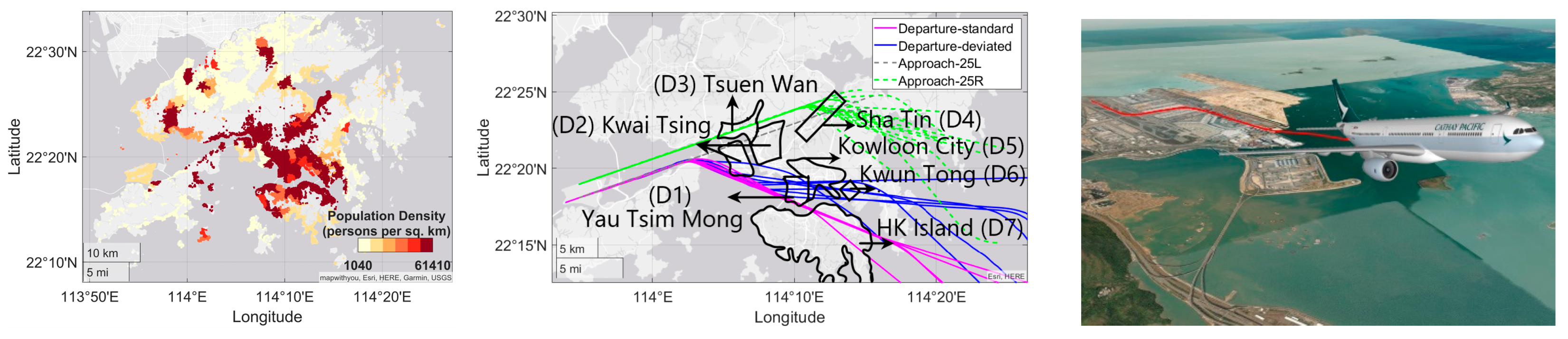
The present section further illustrates the capacity of the aircraft noise prediction methodology to tackle real-life situations by considering actual flight scenarios coming from one of the major international airports, worldwide.

4.1. Context

Hong Kong International Airport (HKIA) is among the busiest airports in the world, ranking 1st and 13th in terms of cargo and passenger traffic, respectively. On the other hand, Hong Kong is the 6th densest city worldwide, and many of its highly populated residential areas are prone to be impacted by air traffic pollution, whether chemical or acoustical. Since HKIA’s current two-runway system has almost reached its maximum operational capacity, a third runway is now being developed so as to cope with the expected growth of air traffic (of about 5% per year). This makes it critical to accurately assess the noise impact by aircraft take-off and landing operations at HKIA on local communities. Such an assessment must account properly for the specificities that characterize the local Hong Kong aviation scene, whether these concern aircraft operations (power settings, flight trajectories) or meteorological conditions. Indeed, because of both the complicated airspace (crowded air traffic, topography, densely populated areas, available routes) and the adoption of specific procedures (e.g., continuous descent approach, CDA [66]), the flight trajectories around HKIA are pretty diverse, and definitely non-standard. In addition, due to its unique geographical location, Hong Kong undergoes important seasonal changes over the year (namely, the summer is hot and very humid, whereas the winter is rather cool and dry.).
To further illustrate the ability of the present approach to tackle real-life scenarios, the present section assesses the noise impact entailed by actual aircraft flying in and out from HKIA, a special focus being put on those Hong Kong’s densely populated areas that are likely to be more exposed to it. The left side of Figure 8 plots the spatial distribution of Hong Kong’s population in 2020 (as provided by the Hong Kong Census and Statistics Department) whereas its center side depicts some typical flightpaths of representative aircraft flying to/from Taipei in 2020 (as provided by the major airline in Hong Kong, Cathay Pacific). The areas depicted in black (namely, D1-D7) are densely populated districts with many aircraft flying over, which the focus is put on here. In that regard, a representative set of aircraft and flightpaths are selected, their noise footprint on the ground being then simulated using the noise prediction platform.
A quick analysis of the air traffic around HKIA in 2021 reveals that the most frequently used aircraft types are A330-343, B787-9 and B777-3ER. We thus here consider both A330-343 and B777-3ER aircraft flying in/out HKIA from/to Taipei (the B787-9 being discarded since its characteristics are not yet incorporated in the ANP database and are rather close to those of A330-343). For each aircraft considered, the operational characteristics and associated flightpaths are excerpted from actual data provided by the airline (Cathay Pacific). Among all available possibilities, specific flights are selected, and their noise impact (SEL) on Hong Kong residential areas is predicted using the present approach. The latter incorporates most features, e.g., it accounts for the atmospheric properties (humidity, temperature, pressure), the installation effects (bank angle), the dynamic grid functionality. On some occasions, additional methodological ingredients are used, e.g., the ground track extension (cf. Section 4.3.2), the thrust approximation (cf. Section 4.3.3). Unless stated otherwise (e.g., Section 4.2.2), the atmospheric conditions correspond to the so-called ISA+10 atmosphere, which is classically used (including for noise certification tests) and is rather close to the yearly averaged meteorological data recorded in Hong Kong. Finally, for helping the reader identifying more easily the various scenarios considered hereafter, each flight is labeled using a specific nomenclature, namely, XYn, where X refers to the aircraft type (“A” for A330-343, “B” for B777-3ER) whereas Y relates to the flight type (“A” for approach, “D” for departure) and n is the subsequent scenario index (1, 2, etc.).
Regarding the aircraft noise exposure in Hong Kong, the solely available data are the official records from HKCAD. The latter come as averaged ground noise levels, which are recorded annually over a few specific locations and integrated over time (irrespective of aircraft movements). In the absence of suitable validation means coming from field tests, all the noise predictions presented hereafter are thus used for illustration purpose. They however deliver insightful information, whether the latter relates to phenomenological aspects (see Section 4.2) or to methodological considerations (see Section 4.3). More precisely, here, we assess the noise impact sensitivity towards various key factors, namely the flight characteristics (flightpath, power settings), the meteorological effects (atmospheric absorption, acoustic impedance), the aircraft type, but also the way to infer them better (flightpath extension, trajectory and/or thrust approximation), etc. Of note, these predictions incorporate the ground effects regardless of the specificities coming from the actual terrain (e.g., landscape, buildings, vegetation, or water), which would be too cumbersome to account for. These specificities are nevertheless expected to be of secondary importance compared to the effects that are primarily sought after, here.

4.2. Phenomenological Aspects

4.2.1. Noise Impact Variability upon the Flight Scenarios

Aircraft operations around HKIA rarely comply with standardized flightpaths, being rather characterized by scattered flight profiles. In that regard, the present section illustrates the variability of aircraft noise impact towards the diversity in flight routes.

Departure Scenarios

We consider those departure routes followed by A330-343 aircraft flying from Hong Kong to Taipei, focusing on those Hong Kong densely populated areas that are located underneath flight corridors (namely, D1, D5, D6, and D7 in Figure 8). Among all corresponding flights available from the database, two specific A330-343 departure flights are chosen upon the high disparity between their characteristics. Indeed, the first aircraft (flight AD1) flies over D1 and D7 districts following a standard route, while the second aircraft (AD2) rather flies over D5 district with a much lower rate of climb (ROC). The left and center sides of Figure 9, respectively, depict the ground track and flight profile of the corresponding routes, which are here plotted up to the nominal maximum altitude of 10,000 ft [37]. The right side of Figure 9 plots the observer grid, as generated using the dynamic meshing technique (cf. Section 2.3.3).
The left and right sides of Figure 10 depict the SEL contours generated by flights AD1 and AD2, respectively. As can be seen, each flight exhibits a rather specific noise signature on the ground, thereby impacting Hong Kong in its own way. This disparity between both flights’ impacts is quantified on the Figure 11, which depicts the differences between the two noise maps (obtained here by subtracting the former from the latter).
Compared to flight AD1 (standard route, higher ROC), flight AD2 (deviated route, lower ROC) has a much higher impact on some of the populated areas, namely districts D1, D5 and D6 (see the right side of Figure 11). More precisely, the excess in SEL raises up to 5dB in districts D1 and D5, whereas it can reach up to 15dB in district D6, which is the most densely populated area in Hong Kong. On the other hand, the opposite holds for other city areas—such as district D7, where the impact of flight AD1 is about 10dB higher than that of flight AD2.
At this stage, it is worth noting that the higher altitude of flight AD1 does not necessarily translate into a lower noise impact on the ground areas it flies over, compared to what happens for flight AD2. For instance, the noise impact by flight AD1 on the D7 district is comparatively higher than that of flight AD2 on the D5 district, although the latter flight travels at an altitude that is half of the former. This can be explained by the difference in the power settings adopted by both aircraft along their respective routes. Indeed, the power settings associated with both flights are depicted in Figure 12, which delineates (in dash-dotted lines) the particular flight phase during which both aircraft pass nearby districts D1 and D5. During this phase, flight AD1 exhibits an engine power that is more than twice that of flight AD2 (whose ROC is suddenly and drastically reduced at that time). This excess of propulsive power translates into a more important noise emission, whose effect cannot be completely mitigated by the longer propagation distance entailed from flight AD1 higher altitude. Independently of the engines power (i.e., noise source amplitude), the flightpath angle (i.e., noise source directivity) may also explain such a comparatively higher noise impact by flight AD1. Indeed, during this flight phase, flight AD2 adopts a lower climb angle than that of flight AD1, as revealed by the flight profiles on the center side of Figure 9. Considering the highly directive patterns of jet noise (whose maximum radiation is aligned with the aircraft axis), this lower flightpath angle by flight AD2 is likely to induce a lower noise impact on the ground. This being said, these more favorable characteristics of flight AD2 (less power, reduced climb angle) do not prevent it to generate a quite substantial noise impact on these areas it flies over rather closely, such as districts D1 and D5.
A similar analysis was conducted for B777-3ER aircraft flying along both the standard and an alternative deviated route, leading to the same observations (see Appendix C).
All the above illustrate well how the variability in departure procedures around HKIA may have a quite large impact on specific, highly densely populated areas of Hong Kong city. From a methodological viewpoint, this underlines the necessity to account as accurately as possible for all flight characteristics when assessing the noise impact by air traffic operations.

Approach Scenarios

Whereas the previous section focused on A330 aircraft departing from HKIA (with their B777 counterpart being documented in Appendix C), this section rather focuses on B777-3ER aircraft at approach. More precisely, we consider the two approach routes to HKIA (namely 25R and 25L), which both pass through three densely populated districts (namely D2, D3, and D4 in Figure 8). Among all B777-3ER aircraft flying from Taipei to Hong Kong in 2020, two specific flights are selected for their high disparity in terms of characteristics (see Figure 13). Whereas the first one (flight BA1) approaches the 25L runway at a higher altitude, the second one (flight BA2) follows the route 25R at a lower altitude. As can be seen, these flight characteristics differences are more prominent at the beginning of the flight sequence, since both aircraft adopt similar trajectories as they get closer to HKIA, to comply with the noise abatement procedures enforced in Hong Kong, namely the Continuous Descent Approach.
The left and right sides of Figure 14 depict the SEL contours generated by these two flights BA1 and BA2, respectively. As for what could be observed with the departure scenarios (cf. Section 4.2.1), each flight impacts differently Hong Kong residential areas. This disparity between their respective noise impact is quantified on the Figure 15, which depicts the differences between the two noise maps (obtained here by subtracting the former from the latter).
Being sandwiched between 25L and 25R routes, the populated D3 district sees its northwestern part impacted more by flight BA2 than by flight BA1 (with a difference in SEL of up to 7.6 dB), whereas the opposite occurs on D3 southern part (where flight BA1 impact exceeds that of flight BA2 by up to 7.3 dB in SEL)—see the right side of Figure 15.
Considering that most of D3 residents are concentrated in its central and southern areas, flight BA1 thus appears to be less environmentally friendly for this district. The same observation holds for the D2 district, whose population concentration is four times higher than that of its D3 counterpart. Being located right underneath 25L route, this district is impacted more by flight BA1, with an excess in SEL of up to 9dB (compared to that of flight BA2). On the other hand, the D4 district appears to be equally exposed to both flights, each inducing an excess of 5–7 dB compared to the other for those observers that are located underneath their respective flightpath. All in all, it appears that these densely populated districts are more exposed to flight BA1, overall. Therefore, the 25R approach route should be privileged whenever the conditions permit (operational, meteorological, etc.).
A similar analysis was conducted for an A330-343 aircraft flying along these two approach routes, leading to the same observations (see Appendix C).
As for the departure scenarios (cf. Section 4.2.1), the above results illustrate further how the approach procedures around HKIA may impact very differently those highly densely populated areas of Hong Kong city.

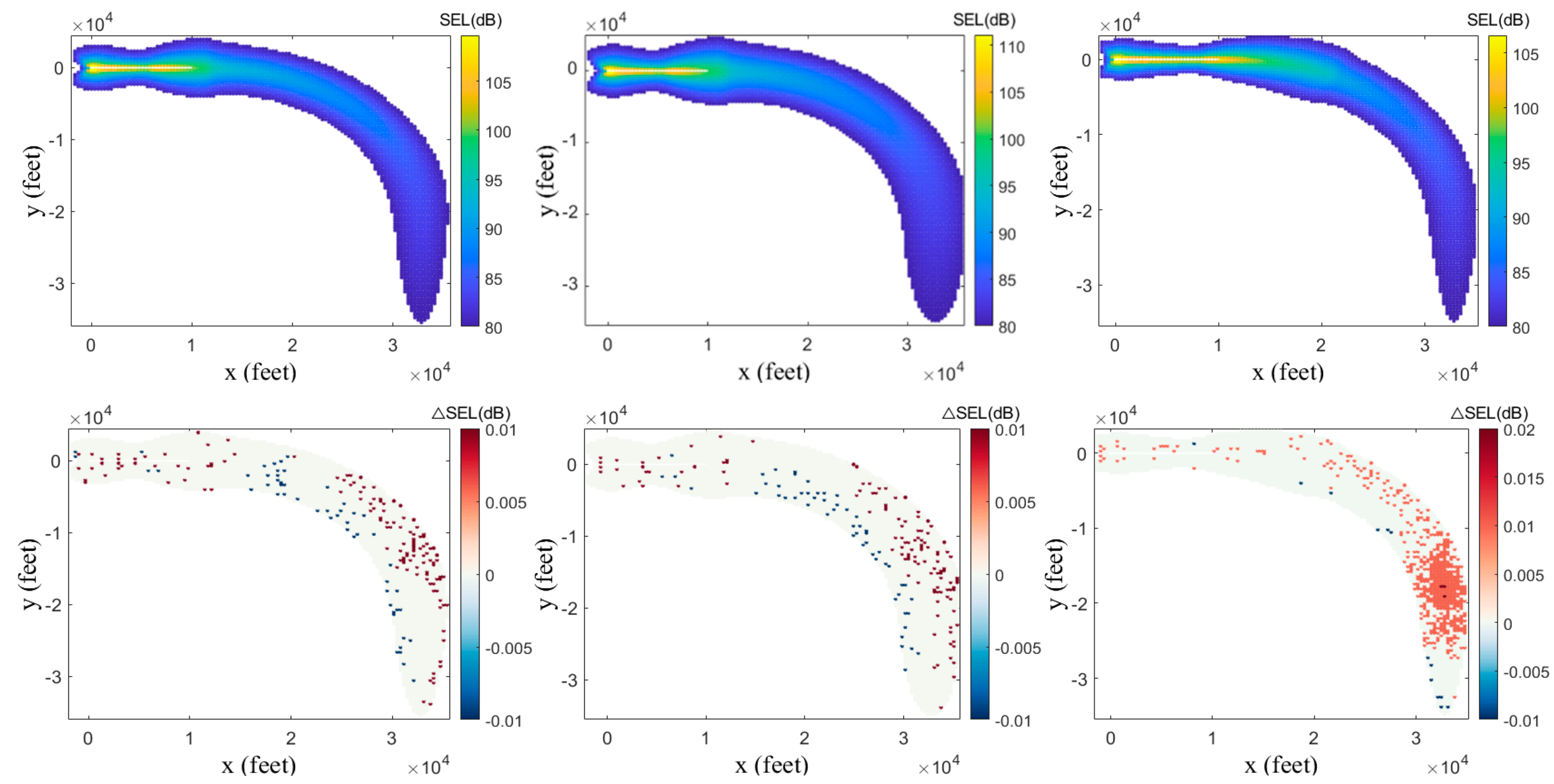
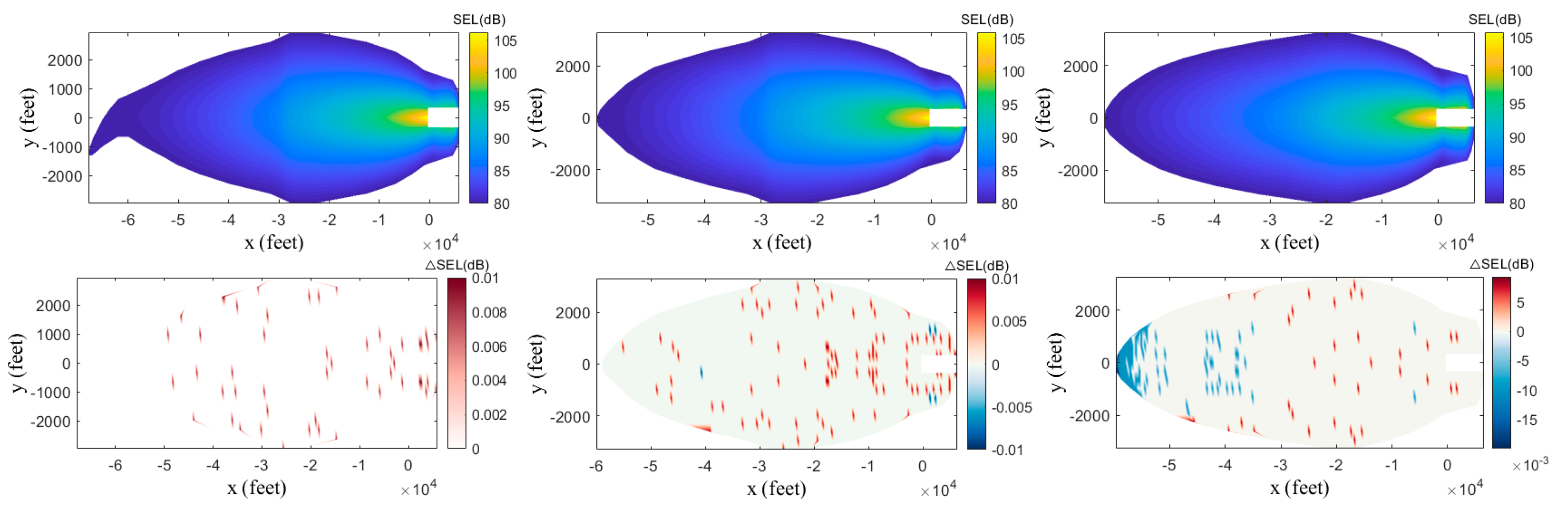
4.2.2. Noise Impact Variability upon the Meteorological Conditions

As said, because Hong Kong usually undergoes important seasonal changes, the local atmospheric conditions may present large deviations compared to the standard ones. For instance, according to the meteorological data records acquired over the past decade by the Hong Kong Observatory and Iowa State University, Hong Kong is characterized by large yearly variations in temperature and relative humidity (which can range from 3 °C to 37 °C and 6.91% to 100% throughout the year, respectively). Moreover, these fluctuations may be important on a much shorter timescale, with large deviations occurring throughout a single day.
The present section illustrates how such a meteorological variability may affect the aircraft noise impact on the ground, for instance, because of the deviations in the atmospheric absorption (which focus is put on, here). To do so, we consider the particular case of an A330-343 aircraft flying from Hong Kong to Taipei along a standard departure route, this flight being successively operated under four specific meteorological scenarios, which reproduce the extrema in temperature or relative humidity one can get in Hong Kong, yearly (see Table 3). For each one of the four scenarios (respectively labeled as AD3, AD4, AD5, AD6), Figure 16 depicts the corresponding SEL on the ground, whose differences are quantified and discussed in the next subsections.

Effect of Temperature

By comparing either cases AD3 and AD4 or cases AD5 and AD6, we first highlight how the noise impact may be altered by variations in temperature (alone), for a given relative humidity. For each pair of cases, Figure 17 depicts the differences in ground noise levels, as obtained by subtracting the SEL map associated with case AD3 (resp. AD5) from that of case AD4 (resp. AD6). As can be seen, such a 28 °C rise in temperature noticeably impacts the ground noise levels, whatever the relative humidity is. This effect on the noise impact appears to be driven by both the observer location and the actual level of relative humidity. When the latter is low (13%), the noise impact is seen to increase (resp. decrease) for those observers that are located close to (resp. away from) the ground track (cf. left side of Figure 17). Oppositely, when the relative humidity is high (100%), a lower (resp. higher) noise impact is recorded for those observers that are positioned close to (resp. away from) the ground track (cf. right side of Figure 17).

Effect of Relative Humidity

Similarly, by comparing either cases AD3 and AD5 or cases AD4 and AD6, we highlight how the noise impact may be altered by the variations in relative humidity (alone), for a given temperature. Figure 18 depicts the differences in ground noise levels, as obtained by subtracting the SEL map associated with case AD3 (resp. AD4) from that of case AD5 (resp. AD6). Whatever the temperature is, such an 87% variation in relative humidity significantly alters the ground noise levels, which now increase everywhere. Again, this effect on the noise impact appears to depend on both the observer location and the actual temperature. When the latter is low (7 °C), the impact is seen to be more important for those observers that are located close to the ground track (cf. left side of Figure 18). Oppositely, under a high temperature (35 °C), the impact is higher for those observers that are positioned further away from the ground track (cf. right side of Figure 18).

Combined Effect of Both Temperature and Relative Humidity

Finally, by comparing cases AD3 and AD6, we illustrate the combined effect of temperature and relative humidity on the noise impact. Figure 19 depicts the differences in ground noise levels, as obtained by subtracting the SEL map associated with case AD3 from that of case AD6. As can be seen, when both temperature and relative humidity increase, the ground noise impact goes higher. For instance, a variation of +9.6 dB is recorded for that observer located at the left/bottom corner of the grid. Notably, this difference represents the arithmetic sum of the ones recorded separately for a variation in temperature alone (−9.1 dB, cf. left side of Figure 17/AD3 → AD4) and in relative humidity alone (+18.7 dB, cf. right side of Figure 18/AD4 → AD6). This illustrates well the dual dependency of the noise impact onto both the temperature and humidity, whose respective effects are cumulative (and may mitigate each other, depending on the situation, cf. Section 2.3.4).
At this stage, it is worth observing that the above results (both trends and numbers) are specific to the present HKIA-based scenario and should not be extrapolated readily to other situations. They however highlight well how important the atmospheric properties may alter the noise impact by air traffic operations, from a phenomenological viewpoint. From a methodological perspective, they underline the crude necessity of accounting properly for the local atmospheric conditions when assessing the noise impact of air traffic operations, especially in those regions that are known to undergo important seasonal variations, such as Hong Kong.

4.2.3. Noise Impact Variability upon the Aircraft Type

The previous sections highlighted how far a given aircraft may see its noise impact varying, depending on its operational conditions (flight route and power settings, meteorological conditions, etc.). Here, we rather explore how, for identical operational conditions, two distinct aircraft may entail different noise impacts. To do so, we consider two of the previous flights, whereas allotting them with a different aircraft type than previously carried out.
Focusing first on departure scenario (cf. Section 4.2.1), we repeat the noise prediction associated with flight AD2 (deviated route, lower ROC), the previous aircraft (A330-343) being now replaced with a (virtual) B777-3ER. Of note, it was checked that such a virtual scenario is realistic, e.g., the B777 engines can deliver the power required by the corresponding A330 flight settings. Figure 20 depicts the SEL maps induced by both cases (respectively labeled AD2 and BD1), along with their difference. As can be seen, B777-3ER aircraft impacts Hong Kong less than its A330-343 counterpart, with noise levels that are lower by about 3 dB over most residential areas. This trend is however inverted further away from the ground track, with an excess noise by the B777 of up to 5 dB recorded over some more remote locations (which are nevertheless sparsely populated).
At this stage, one could wonder about the exact reason for such an inverted trend, in terms of noise impact by both aircraft with respect to the distance to the ground track. Indeed, both AD2 and BD1 scenarios differ only by the aircraft type (i.e., noise source), all other parameters being strictly identical (flightpath, power settings, atmospheric absorption, etc.). However, as can be inferred from the NPD database (see Figure 21), both aircraft see their noise levels varying (i.e., decreasing) differently along the propagation distance. In particular, although they are less than the A330 ones at short distances, the B777 noise levels emerge more further away. This can be related to the atmospheric attenuation effects, which are to impact differently both noise signatures depending on their respective spectral content.
Focusing now on approach scenarios (cf. Section 4.2.1), we repeat the noise prediction associated with flight BA1 (25L runway, lower altitude), the previous aircraft (B777-3ER) being now replaced with a (virtual) A330-343 counterpart. Notably, here too, it was checked that such a virtual scenario is realistic, e.g., the A330 engines can deliver the power required by the corresponding B777 flight settings. Figure 22 depicts the SEL maps induced by both flights (respectively labeled BA1 and AA1), along with their difference. As can be seen, compared to its B777-3ER counterpart, A330-343 aircraft impacts Hong Kong less, with noise levels that are systematically lower—wherever the observer location is. In particular, the populated D6 district sees its noise impact reduced by as much as 5 dB when flown over by an A330 instead of a B777.
The above results illustrate how aircraft noise prediction methods such as the one presented here constitute not only a useful diagnostic tool but also a powerful predictive means. Indeed, beyond simply allowing to measure the noise impact by existing aircraft operations around major airports, such kind of tool can also help better planning them. This is of critical importance when new airport developments are on their way, as is currently the case with HKIA.

4.3. Methodological Aspects

Whereas the previous sections primarily focused on phenomenological aspects of aircraft noise impact, we here discuss the prediction process under a more methodological angle.

4.3.1. Accounting for the Bank Angle

In the previous sections, all noise predictions accounted for the engine installation effects (cf. Section 2.3.2), which were incorporated through the bank angle. One can however wonder about how big their influence on the noise impact is, that is, how critical it is to integrate them in the calculation process. To do so, we repeat the noise prediction of flight AD2 (which undergoes more banked turns than flight AD1), the bank angle effect being either incorporated or neglected in the calculation. Figure 23 compares the SEL maps obtained with (left) and without (center) the bank angle effect, along with their difference (right).
As can be seen, when the aircraft is engaged into a banked turn, most of the observers that are located on the same (resp. opposite) side of the turn are exposed to lower (resp. higher) noise levels (see what happens on the right side of Figure 23, for instance). This trend, however, is inverted for the small fraction of observers that are located very close to the ground track. All this can be easily explained upon the respective way each observer perceives the relative depression angle, which is either increased or decreased because of the bank (see Figure 2, wing-mounted engines polar). From another hand, this effect of the bank angle appears to be rather modest, with noise differences of less than 0.3 dB overall. This number appears to be even lower for flight AD1, whose straighter flightpath naturally leads to a less important effect of the bank angle (cf. Appendix C).
A similar analysis was conducted for B777-3ER aircraft flying along different departure routes, leading to the same trends (see Appendix C).
On one hand, the above results confirm that the noise impact by an aircraft does not vary much during a banked turn, which explains why this aspect is often neglected in the prediction [62]. On the other hand, however, these results illustrate how one can further refine the accuracy of the noise prediction by incorporating still more additional effects, even though they are of secondary importance.

4.3.2. Extending the Flightpath Cut-off Limit

In the previous sections, all noise predictions relied on the classical approach of incorporating only those flightpath segments that would fall under an (arbitrary) reference altitude of 10,000 ft. As discussed previously (see Section 2.3), this is likely to induce a bias in the noise prediction because some of the contributing flight segments would then be ignored. In Section 4.2.1, for instance, flight AD1 (standard route, higher ROC) reaches the limit altitude much earlier than flight AD2 (deviated route, lower ROC), which may translate into a predicted noise impact that becomes less than the actual one. To illustrate this point, the noise prediction of flight AD1 is here refined, being now conducted using the automatic flightpath extension proposed in Section 2.3.3 (i.e., all contributing flight segments are incorporated in the prediction). As revealed by Figure 24, the noise impact by such an extended flight (labeled hereafter AD1-ext) goes on increasing beyond its former (10,000 ft limited) value until it reaches a plateau (around an altitude that is almost twice, i.e., 18,670 ft). This leads to a ground SEL that is higher, with differences of up to 30 dB at some locations (see right side of Figure 24).
The above result illustrates well how aircraft noise predictions can be biased by the arbitrary limitation of the route beyond a given reference altitude. In turn, it shows how to avoid such a bias by using a dynamic flightpath extension, such as the one proposed here.

4.3.3. Approximating the Flightpath and/or Power Settings

As said, aircraft operations around HKIA rarely comply with standardized flightpaths, being rather characterized by scattered flight profiles (cf. Figure 25). In the absence of any FDR (Flight Data Recorder) inputs, modeling these flights requires using radar information and inferring power settings, for instance using the model proposed in Section 2.3.1. Radar data, however, are of limited accuracy [67,68], and it is not rare that they noticeably differ from the actual (FDR) ones. These discrepancies may question the validity of either the thrust estimation (which requires knowing accurately both the acceleration and attitude of the aircraft, cf. Section 2.3.1) or of the noise prediction (which relies on the correct knowledge of the aircraft-to-ground distance, i.e., flight trajectory). Assessing this point is the matter of the present section.
We here consider two pairs of specific flights, each relating to an identical aircraft and mission (B777-3ER or A330-343 aircraft flying from Hong Kong to Taipei) whereas presenting rather different characteristics in terms of flight profile (cf. Figure 25) and/or engine power evolution (cf. top right of Figure 26, Figure 27, Figure 28 and Figure 29). Here, we solely consider departure scenarios since those are primarily concerned with pure propulsive noise, for which a correct estimation of the thrust is vital. We first assess the validity of the thrust estimation alone, this being performed by applying Equations (2)–(4) to accurate trajectory inputs coming from FDR data. The latter are then replaced with their (less accurate) radar data counterparts, which are extracted from FlightRadar24 website (business version). The objective is to assess how far the radar data inaccuracies may impact the thrust estimation, and ultimately, the noise prediction. Of note, since the present radar data solely provide the aircraft ground speed, we infer its airspeed counterpart by adding to it a headwind component (whose value is arbitrarily taken as 8 kt [49], for a lack of better information on wind profiles). Besides, here, the atmosphere characteristics are based on the average values recorded in Hong Kong for 2020.
For both pairs of flights (hereafter labeled as BD2, BD3 and AD7, AD8), the thrust evolution is first estimated using the actual (FDR) data, its averaged value (labeled as “smoothed thrust”) being then compared with its actual counterpart (labeled as “actual thrust”). As can be seen on the top right of Figure 26, Figure 27, Figure 28 and Figure 29, the agreement is fairly good, whatever the scenario is. In particular, for both B777 flights (BD2, BD3), the estimation is very satisfactory, with an estimated thrust that matches the actual one almost perfectly (compare black and red curves on the top right of Figure 26 and Figure 27, respectively). This good match slightly degrades for both A330 flights (AD7, AD8), whose actual and predicted thrust differ in some places (compare again the black and red curves on the top right of Figure 28 and Figure 29, respectively). These discrepancies come from the much less monotonic character of the flight (and, thus, power) settings, whose important variations make the thrust estimation more challenging. Despite such a fussy timeline of the power settings (which turned out to be the more complicated ones, among all the considered cases), the thrust estimation is still very favorable, delivering trends that are quite close to the actual result. This fair character of the thrust estimation naturally translates into a fair prediction of the aircraft noise impact, as shown on the bottom of Figure 26, Figure 27, Figure 28 and Figure 29: whereas the left image plots the actual SEL map (predicted using the actual thrust), its center counterpart depicts the error incurred by the thrust estimation (obtained by subtracting the former SEL map from the one predicted using the estimated thrust). Whatever the considered flight is, this error on the SEL prediction ( Δ S E L ) is mostly in the range of ± 1dB: whereas it can reach up to ±2.5 dB at the beginning (start-of-roll) and/or the end of the flight sequence (standard limit altitude of 10,000 ft), the Δ S E L never exceeds ± 1dB in the rest of the flight sequence. Such discrepancies, which primarily reflect the accuracy limitations of FDR data (e.g., lack of discretization, absence of information on flap settings, etc.), are deemed to be acceptable for such low-order modeling of the thrust.
Independent of the thrust model itself, the uncertainties that weigh on the flight settings (trajectory, airspeed) provided by the radar data may however entail additional errors. To illustrate this point, we here re-assess the thrust estimation, its FDR-originated inputs being now replaced with their radar data counterpart. The latter may indeed importantly differ from the former, whether this concerns the flight profile (cf. top/left images of Figure 26, Figure 27, Figure 28 and Figure 29) or the airspeed (cf. top/center images of Figure 26, Figure 27, Figure 28 and Figure 29). Notably, only the actual ground track appeared to be accurately reproduced by the radar data, across all cases. For each flight, the cumulative effect of all these discrepancies onto the aircraft noise is again quantified in terms of Δ S E L maps (see bottom right image of Figure 26, Figure 27, Figure 28 and Figure 29). The latter are obtained by subtracting the actual ground noise levels (predicted using the FDR inputs, among which is the actual thrust) from their approximated counterpart (predicted using the radar-originated inputs and subsequently estimated thrust). Overall, the fidelity of the noise prediction appears to be driven by the radar data accuracy. Considering for instance the BD2 flight, one can see that the radar-originated flight profile, airspeed and thrust do not devoid much from their actual counterparts (the early take-off excepted). The resulting bias on the noise prediction is fairly low (cf. bottom right of Figure 26), with deviations of less than 0.5 dB for most of the flight sequences (except at the take-off start, where radar uncertainties entail noise discrepancies of about 15 dB). For BD3 flight, the radar-estimated altitude is higher than its actual value throughout the entire flight sequence (so much that the 10,000 ft limit altitude is reached earlier), which results in slightly higher error levels on the noise prediction ( Δ S E L ~ 1 dB, overall). Notably, the radar-based estimated thrust still agrees well with both its actual and its FDR-estimated counterparts (compare the blue, red and black curves on the top right of Figure 27). Only at the start and at the end of the flight sequence, this agreement on both the thrust estimation and the noise impact appears to be less satisfactory. This may tend to indicate that, here, the radar data inaccuracies primarily weigh on the thrust prediction, more than on the propagation aspects (e.g., the aircraft-to-ground distance). Notably, because their respective discretization levels differ, FDR and radar data exhibit slightly different start-of-roll point, lift-off point and endpoint. Similar trends are observed for the AD7 flight, whose radar-originated airspeed appears to be less accurate than its flight profile counterpart (cf. left and center images on top of Figure 28, respectively). Combined with the fuzzy evolution of the power settings, these radar data inaccuracies challenges still more the thrust estimation (compare the blue, red and black curves on the top right of Figure 28). Besides, such a variability of the radar data airspeed is very likely to incur a different exposure duration to the noise associated with each flight segment, thereby further affecting the entire prediction, ultimately. Despite all these discrepancies, however, the noise impact is predicted rather accurately, with error levels that fall in the range of [−2; 0] dB (except again near the start-of-roll point, where differences reach 40 dB). Finally, AD8 flight reveals how radar data may resemble their actual counterparts (cf. left and center images on top of Figure 29) whereas entailing still more bias on the thrust estimation (compare the blue, red and black curves on the top right of Figure 29). At this stage, however, it is believed that the lesser discretization of the radar data (compared to their FDR counterpart) might explain such discrepancies on the thrust, whose estimation might then be still more challenged by the fuzzy timeline of the power settings. Whatever the reason for such biases on the thrust estimation, the overall impact on the noise prediction is still acceptable, with Δ S E L that never goes under −3 dB (cf. bottom right of Figure 29).
All in all, the above results illustrate the ability of the noise prediction method (and its underlying thrust model) to solely rely on radar data, thereby allowing to handle flightpaths that differ from standard ones whenever FDR information is unavailable.

5. Conclusions and Perspectives

The present study focuses on the noise impact by aircraft operations around major airports. To this end, an aircraft noise prediction platform was developed, which relies on state-of-the-art functionalities as well as more specific, innovative features. More precisely, the method classically relies on the Aircraft Noise and Performance (ANP) database and its Noise–Power–Distance (NPD) table. The latter, however, are known to suffer from restrictive assumptions which limit their application to simplified situations. For instance, the ANP database is built upon standardized scenarios of aircraft operations (aircraft types, flightpaths, power settings, atmospheric conditions, etc.). Besides, its NPD component relies on the simplistic scenario of a punctual noise source radiating within a homogeneous free field. Last but not least, the ground observer is assumed to be located right underneath the aircraft, with the latter flying with a constant speed and power settings along an infinite horizontal flightpath. To alleviate all these limitations, the present method incorporates several functionalities, some of which are specific to the present study. These features aim at (i) refining the noise emission stage (e.g., source intensity and directivity) as well as (ii) improving the propagation phase. Regarding for instance the refinement of the aircraft noise source, an innovative method is proposed, which allows inferring the engine power solely from the aircraft flightpath characteristics (whose access is much easier than that of Flight Data Recorder). Besides this, a functionality is introduced which allows extending automatically and dynamically the flightpath, thereby avoiding an arbitrary truncation of the aircraft noise emission as well as ensuring an accurate representation of its subsequent propagation. The latter propagation is also refined through the proper incorporation of the noise attenuation effects induced by any realistic, non-standard atmosphere. Other specific features are incorporated into the method, which aim at improving its efficiency (accuracy and execution speed). For instance, a recursive, dynamic grid refinement technique offers to optimize the number and distribution of ground observers, thereby maximizing the results accuracy whereas minimizing the prediction time.
The noise prediction method and subsequent computational platform are successfully validated using several benchmark cases of increasing representativeness. They are then applied to several realistic scenarios coming from actual aircraft operations around Hong Kong International Airport (HKIA). Specific comparative analyses are conducted, which allow highlighting the variability of the noise impact by aircraft, depending on their type (A330, B777) and/or operational conditions (power settings, meteorological conditions, routes, banks, etc.). From a phenomenological viewpoint, results allow discriminating the more prominent drivers, namely, the aircraft flightpath characteristics, the engine power settings, etc. It is also shown how important the meteorological conditions can be, because of the specific atmospheric attenuation effects they entail. Oppositely, the engine installation effects (assessed through the aircraft bank effects) appear to be of secondary importance. From a methodological perspective, the results showcase the capacity of the present approach to handling real-life situations, including when the latter greatly differ from the standardized scenarios underlying the ANP database. They also illustrate how noise prediction methods/platforms such as the present one may help in guiding the further expansion of airport operations and/or infrastructures (as is currently the case with HKIA).
With this end in view, it is planned to further improve the present approach, whether it is by refining still more its noise emission stage (e.g., assessing better the aircraft power settings using the Base of Aircraft Data database, BADA [69,70,71]), or by strengthening further its propagation phase (e.g., incorporating variable atmospheric conditions such as wind effects [72,73,74]). Last but not least, it is envisioned to extend the tool’s capacities from an aircraft to a fleet level [75] so as to allow better optimizing air traffic operations.

Supplementary Materials

The following are available online at https://www.mdpi.com/article/10.3390/aerospace8090264/s1.

Author Contributions

Conceptualization, S.R. and C.W.; methodology, S.R. and C.W.; software, C.W. and S.R.; validation, C.W. and S.R.; formal analysis, S.R. and C.W.; investigation, C.W. and S.R.; resources, C.W. and S.R.; data curation, S.R. and C.W.; writing—original draft preparation, C.W.; writing—review and editing, S.R.; visualization, S.R. and C.W.; supervision, S.R.; project administration, S.R.; funding acquisition, S.R. Both authors have read and agreed to the published version of the manuscript.

Funding

This research received no external funding.

Institutional Review Board Statement

Not applicable.

Informed Consent Statement

Not applicable.

Data Availability Statement

The data presented in Section 3 are openly available online: https://www.ecac-ceac.org/images/documents/ECAC-Doc_29_4th_edition_Dec_2016_Volume_3_Part_1.pdf. Besides, publicly available datasets used in Section 3 and Section 4 can be found here: https://www.easa.europa.eu/document-library/type-certificates and https://www.flightradar24.com/. Some of these data are made available to the reader, as Supplementary Material (namely the radar data of flights BD2, BD3, AD7 and AD8 in Section 4). The FDR data used in Section 4 cannot be made publicly available, due to their proprietary nature (Cathay Pacific airline).

Acknowledgments

The present research is a byproduct of a cooperative effort between Cathay Pacific airline (CX) and the Hong Kong University of Science and Technology (HKUST). The authors are grateful to Cathay Pacific for sharing with HKUST some of the flight data excerpted from CX aircraft operations around HKIA airport. Moreover, the authors are thankful to Rhea Liem and Dajung Kim (HKUST) for their support in accessing the data.

Conflicts of Interest

The authors declare no conflict of interest.

Appendix A. Integrated Thrust Equation for the Aircraft at Roll and Aloft

Appendix A.1. Integrated Thrust Equation

We here derive an integrated expression of the engine(s) thrust required for the aircraft to remain in dynamic equilibrium, either aloft (in-flight segments) or on the ground (ground-roll segments). To do so, we consider a virtual situation in which the aircraft is exerted all typical forces (including the ground reaction, which shall vanish automatically in the air). Assuming that the aircraft undergoes a straight accelerated motion, we derive the longitudinal equations of motion (EOM). Once projected along the so-called stability axes (i.e., parallel and perpendicular to the airflow direction, see Figure A1), these EOM are respectively given by:
Figure A1. Forces exerted on the aircraft, as depicted in its longitudinal (left) or lateral (right) planes. Angles associated with the projection in the Earth (x, y, z) and aircraft stability (x’, y’, z’) reference frames: Angle-of-attack ( α ), flightpath ( γ ) and bank ( ϕ ) angles, along with the elevation ( β ) and depression ( φ ) angles.
Aerospace 08 00264 g0a1
m a = T c o s α D + ( R W ) s i n γ F R c o s γ
0 = T s i n α + L c o s ϕ + F R s i n γ + ( R W ) c o s γ
In the above equations, m and W, respectively, stand for the mass and weight of the aircraft, whose (average) acceleration is a . On the other hand, α , γ and ϕ stand for the aircraft’s angle of attack, flightpath and bank angles, respectively. Of note, the bank angle refers to the angle between the Earth reference frame’s horizontal axis (y) and that of the aircraft’s stability reference frame (y’), whose angle with the aircraft-to-observer noise propagation path corresponds to the depression angle ( φ ). Aside from that, T ,   L and D   are the propulsive (thrust) and aerodynamic (lift and drag) forces. R and F R are the two components of the runway reaction, namely the vertical reaction and the roll resistance, which are related through the friction coefficient characterizing the runway, μ F
F R = μ F · R
As a reminder, a typical value for this friction factor is 0.02 (resp. 0.4) for a dry concrete runway without (resp. with) brakes applied.
By combining Equations (A3) and (A2), one can express the ground vertical reaction as
R = W c o s γ L c o s ϕ T s i n α c o s γ + μ F s i n γ
When introducing the lift and drag coefficient (CL, CD), one can then express the drag in terms of the lift alone
D = L · C D C L
One can legitimately assume that the aircraft’s angle of attack is small (that is c o s α   ~   1 and s i n α   ~   0 ), which further simplifies the above relationships. After a few developments, the thrust can be expressed as
T = m [ a + g ( μ F c o s γ + μ F s i n γ ) ] + L [ C D C L + c o s ϕ · ( s i n γ μ F c o s γ c o s γ + μ F s i n γ ) ]

Appendix A.2. Particular Case of in-Flight Segments

When the aircraft is aloft, the ground reaction is nil ( μ F = 0 ), and Equation (A6) becomes
T = m [ a ] + L [ C D C L + c o s ϕ · ( s i n γ c o s γ ) ]
Considering that the lift equals the weight corrected from the simultaneous projection of flightpath and bank angles
L = W c o s γ cos ϕ
Equation (A6) then becomes
T = m [ a + g ( C D C L · c o s γ cos ϕ + s i n γ ) ]
Of note, all parameters appearing in the above equation are readily available from the flight data and/or ANP database.

Appendix A.3. Particular Case of Ground-Roll Segments

On the other hand, when the aircraft is on the ground roll ( γ = ϕ = 0 ), Equation (A6) becomes
T = m ( a + g μ F ) + L ( C D C L μ F )
Expressing the lift force in these conditions is less straightforward, and requires developing an alternative lift model [57]. To do so, we start from the definition of lift
L = ( 1 2 ρ S C L ) V T A S 2
where ρ is the air density, V T A S indicates the true airspeed of the aircraft, S is the wing area and C L is the lift coefficient. Assuming that the wing can be considered as a thin airfoil, the lift coefficient can be classically related to the angle of attack, α (which is supposed to be small enough).
C L = C L , 0 + C L , α α
where C L , 0 stands for the zero-lift coefficient and C L , α is the lift coefficient slope. Assuming that the aerodynamic settings (α, S) and the atmospheric conditions ( ρ ) do not vary during the ground roll (i.e., C = 1 2 ρ S C L = c o n s t ), Equation (A11) turns into a parabolic equation of the aircraft speed (alone)
L = C · V T A S 2
At the lift-off point, the ground reaction vanishes and the lift strictly equals the aircraft weight, W
W = L = C · V L O F 2
where V L O F is the lift-off speed of the aircraft. By neglecting any variation of the aircraft weight during the ground roll, one can thus re-express the lift force as
L = W · ( V T A S V L O F ) 2
All in all, Equation (A6) then becomes
T = m { a + g [ C D C L · ( V T A S V L O F ) 2 + μ F ( 1 ( V T A S V L O F ) 2 ) ] }
Here too, all parameters appearing in the above equation are readily available from the flight data and/or ANP database.

Appendix B. Further Illustration of the Noise Prediction Process and of Its Validation against Reference Cases

This section further illustrates the validation cases provided in Section 3.1, one of which is selected and documented more thoroughly.
Figure A2 depicts the routes (departure and approach, either straight or curved) as well as the set of observers (namely R1–R17) used for all cases [62]. For more details about the other parameters (flightpath, meteorological conditions, power settings, airspeed, etc.), the reader is referred to Ref. [62]. Among the various cases listed, we here specifically focus on the JETWDS configuration (i.e., a wing-mounted jet engines aircraft flying along a straight departure route), whose relevant observers as those labeled R1–R5. Figure A3 depicts the time trace of various key quantities, as recorded for each observer along the flight evolution, which is broken down in terms of flight segments, either ground-roll (1–9) or airborne (10–29). These key quantities constitute the main ingredients of the noise prediction process, namely the baseline noise level perceived by each observer (Figure A3a) and its further adjustment through the cumulative corrections introduced in Section 2.2 (Figure A3b–g). The final result is provided in Figure A3h, which also quantifies the error made with the reference solution [62]. This breakdown of the noise prediction process is summarized hereafter, for illustration and validation purposes.
Figure A2. Departure and approach routes for reference cases, with the associated observers.
Aerospace 08 00264 g0a2
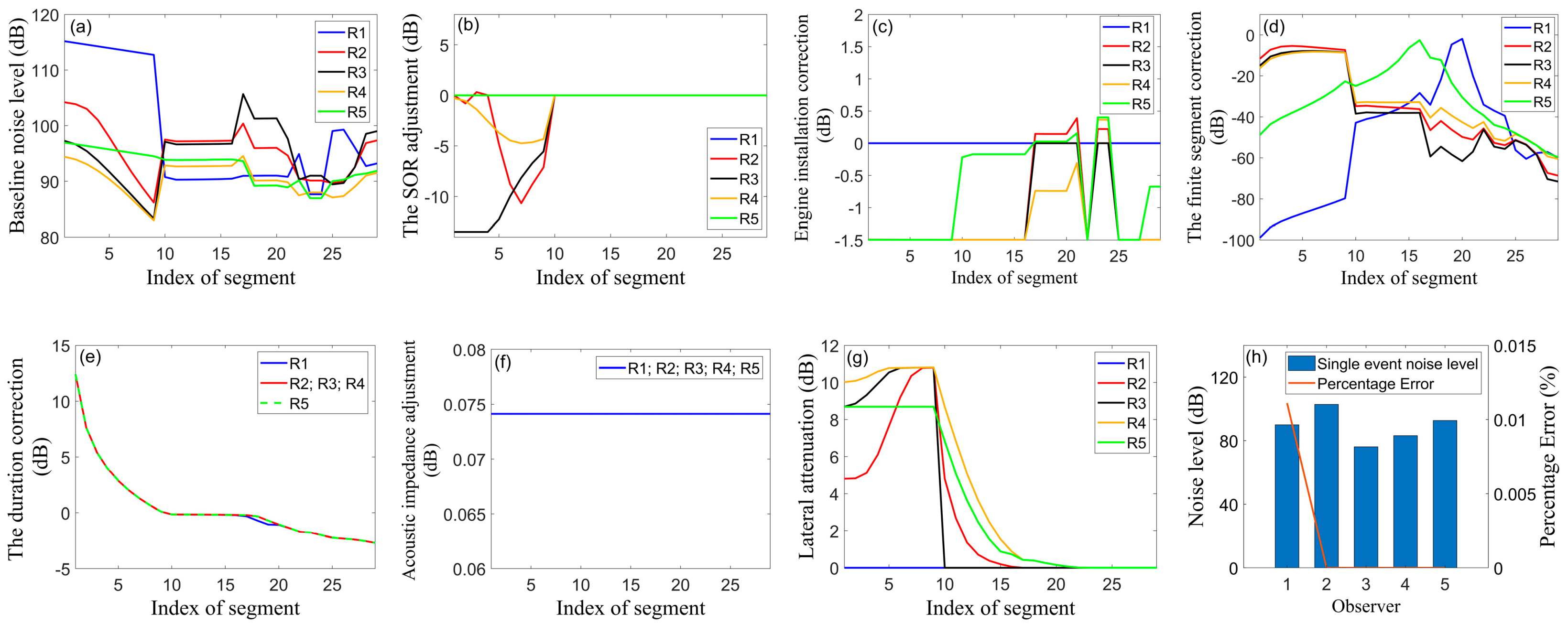
  • Baseline noise level (cf. Figure A3a): Originated from the NPD database, this quantity represents the noise that would be perceived by each selected observer if the aircraft was flying according to a standard scenario (cf. Section 2.2). It was checked that the associate prediction results agree well with the reference values [62], the maximum errors being less than 10 5 % . Since the JETWDS case corresponds to a non-standard flight, these baseline noise levels must be refined through successive correction terms (see below).
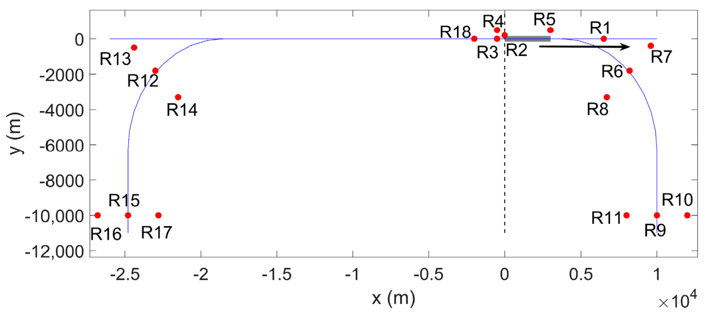
  • Start-of-roll directivity adjustment (cf. Figure A3b): This correction accounts for the highly directive pattern of the jet noise at take-off, which impacts more especially those observers that are located upstream the ground roll segments (cf. Section 2.2). Logically, the effect is nil for these observers that are located downstream (i.e., R1 and R5). Here too, the predicted results match well the reference values, with a maximum error of less than 10 5 % .
  • Engine installation correction (cf. Figure A3c): This correction accounts for the lateral directivity patterns induced by the engine installation effects, which depend on the relative depression angle seen by each observer (cf. Section 2.3.2). Logically, the effect is nil for those observers that are located right underneath the airborne segment (e.g., R1). Again, the predicted values compare favorably against their reference counterparts, with an error of less than 10 9 % .
  • Finitesegment correction (cf. Figure A3d): This correction accounts for both (i) the finite nature of each concerned flight segment and (ii) its relative position with respect to the observers. The effect is more important for those observers that are located away from the flight segment, whose perceived noise is then corrected from the loss incurred by the respective propagation distance. Here too, the calculation results are in good agreement with the reference ones, leading to a maximum error of less than 1%.
  • Duration correction (cf. Figure A3e): This correction translates the variation in the noise exposure duration, which logically varies with the fly-over time and, thus, the aircraft speed. In the present case where the aircraft continuously accelerates (from 0kt at the start-of-roll point) and eventually exceeds the standard value of 160kt (for which the correction is nil), this effect decreases monotonically. Here too, the prediction result is very close to the reference one, with errors in the range of 10 12 % 10 2 % .
  • Acoustic Impedance adjustment (cf. Figure A3f): This correction translates the impact of atmospheric effects (cf. Section 2.3.4), which are solely driven by the local meteorological conditions, thereby affecting all observers equally. Here, no error is recorded.
  • Lateral attenuation (cf. Figure A3g): This correction accounts for the lateral attenuation induced by the ground presence (cf. Section 2.2). Logically, this effect does not impact those observers that are located right beneath the flightpath (here, R1 and R3 for airborne segments 10-29). The other observers are impacted differently, depending on their respective (lateral) distance to the aircraft, as well as on the nature of the flight segment considered (airborne or ground roll [49], e.g., R2-R4 for segments 9 and 10, respectively). Again, the predicted values match the reference ones, with maximum errors of less than 10 1 % .
  • Single event noise level (cf. Figure A3h): This quantity represents the cumulative noise level perceived by each observer, once the contributions coming from all segments are summed up into a single noise event. As can be seen, the prediction is very close to the reference, with errors in the order of zero (except for the R1 observer, for which an error of about 0.011% is recorded).
Figure A3. Breakdown of the noise prediction process, as illustrated for the JETWDS validation case (all in dB). Baseline noise level (a), start-of-roll directivity adjustment (b), engine installation correction (c), finite segment correction (d), duration correction (e), acoustic impedance adjustment (f), lateral attenuation (g), single event noise level (h).
Aerospace 08 00264 g0a3

Appendix C. Further Illustration of the Noise Impact Dependency towards Real-Life Operations

This section first focuses on the noise impact incurred by a B777-3ER (resp. an A330-343) aircraft departing from (resp. approaching) HKIA, thereby mirroring the discussion of Section 4.2.1. In a second time, the effect of banked turn is assessed on these various flights.

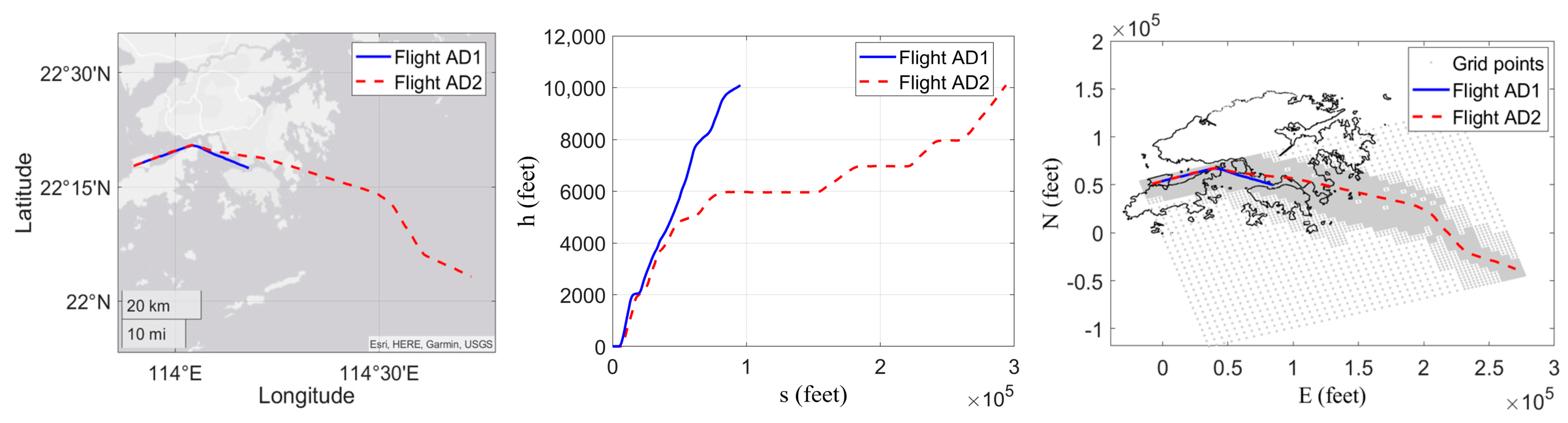
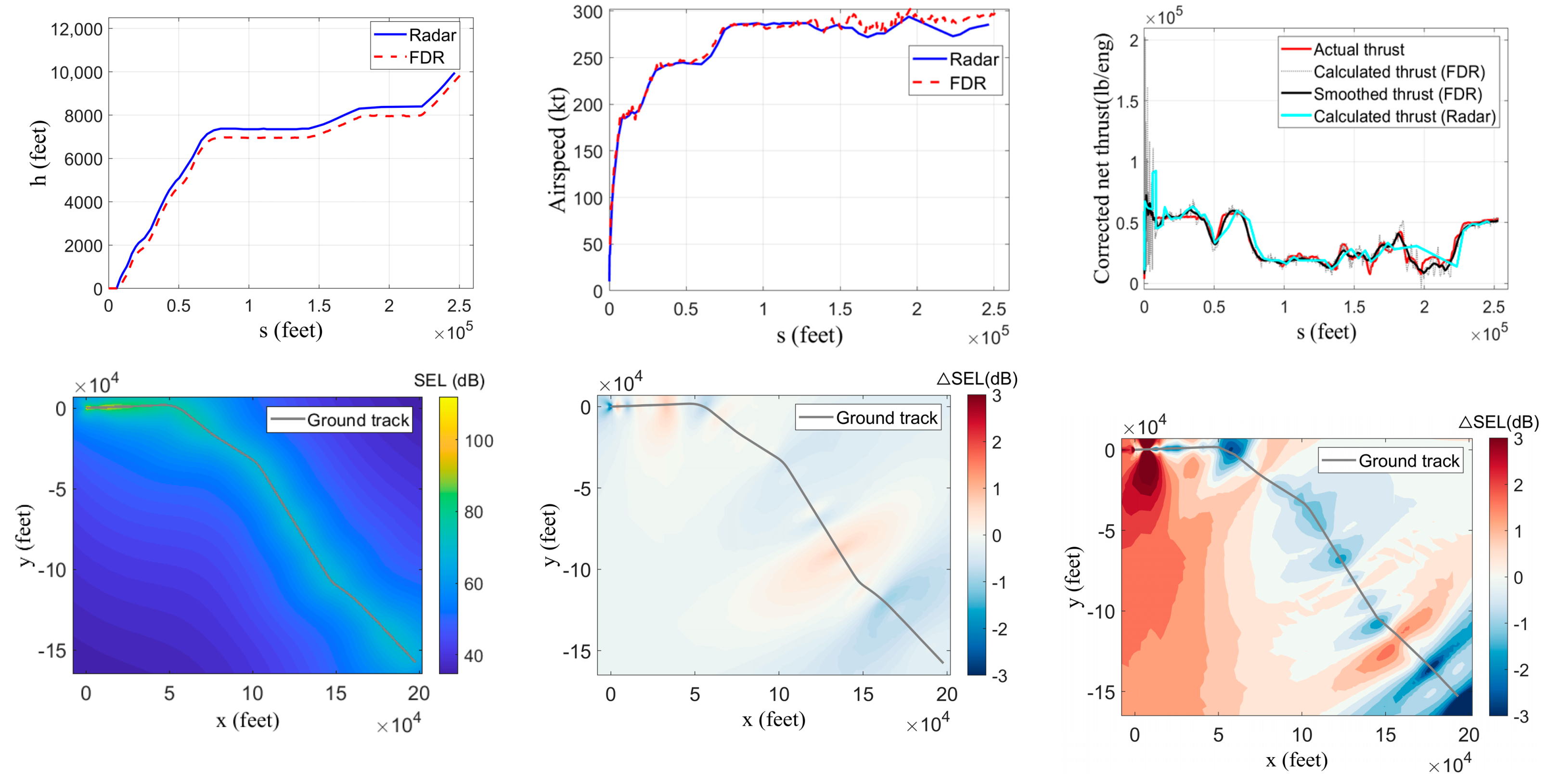
Appendix C.1. Noise Impact Incurred by B777-3ER Aircraft Flying along Two Departure Routes

Regarding the departure scenario, we select two specific B777-3ER flights with very distinct characteristics, and we assess their respective noise impact on three densely populated districts (namely D1, D5, and D7) that they both fly over. Whereas the first flight (labeled BD4) flies over districts D1 and D7 along a standard route with a high rate of climb (ROC), the second one (BD5) passes over district D1 at a lower altitude (see Figure A4).
Figure A4. B777 aircraft departing from HKIA. Flights BD4 and BD5 respective routes (left: ground track, center: flight profile) and corresponding ground observers (dynamic grid, right).
Aerospace 08 00264 g0a4
Figure A5 depicts the SEL contours generated by flights BD4 (left) and BD5 (center) along with their difference, which is obtained by subtracting the former from the latter (right).
Figure A5. B777 aircraft departing from HKIA. Noise impact (SEL) generated by flight BD4 (left) and BD5 (center) over Hong Kong city, along with difference (∆SEL) between both results (as obtained by subtracting the former from the latter, right).
Aerospace 08 00264 g0a5
Compared to flight BD4 (standard route, higher ROC), flight BD5 (deviated route, lower ROC) impacts less some of the populated areas, with noise levels that are lower by around 4 dB in D1 and D5 districts, and by about 7.5 dB in the western part of D7 district. The opposite trend is observed to occur in the eastern part of D7 district, where flight BD5′s impact exceeds that of BD4 by up to 13 dB in SEL (see Figure A6).
As was observed in Section 4.2.1 for Airbus-related flights, the lower altitude of a given flight (here BD5) does not automatically entail a higher noise impact on the ground. For instance, even though flight BD5 passes over D1 district at a lower altitude than its BD4 counterpart, it results in a smaller noise footprint over this area. Here too, this is likely to be explained by the difference in the power settings (i.e., engine thrust) characterizing both aircraft along their respective routes. For instance, Figure A7 compares the time history of the thrust delivered by the two aircraft, with a focus put on that specific flight phase where they both pass nearby D1 and D6 districts (highlighted with vertical dash-dotted lines). At that time, flight BD5 exhibits a propulsive power that is almost one-third of its BD4 counterpart. This is likely to incur a comparatively much lower noise emission for BD5 flight, whose lower noise attenuation (short propagation distance) is then favorably balanced. In addition, here again, the smaller ROC exhibited by flight BD5 is likely to diminish its noise footprint, compared to its BD4 counterpart whose higher flightpath angle somehow exacerbates its noise impact (jet noise directivity). All in all, these two features of flight BD5 (lower power setting, smaller ROC) suffice to offset the detrimental effect entailed by its lower altitude (reduced noise attenuation), when flying over D1 and D6 districts.
Figure A6. Difference in SEL (∆SEL) between flights BD4 and BD5 (closer view).
Aerospace 08 00264 g0a6
Figure A7. Power settings (engine thrust) evolution of flights BD4 and BD5.
Aerospace 08 00264 g0a7
As for what could be observed with the A330 aircraft (cf. Section 4.2.1), the above analysis further illustrates how HKIA departure procedures may impact very differently those highly densely populated areas of Hong Kong.

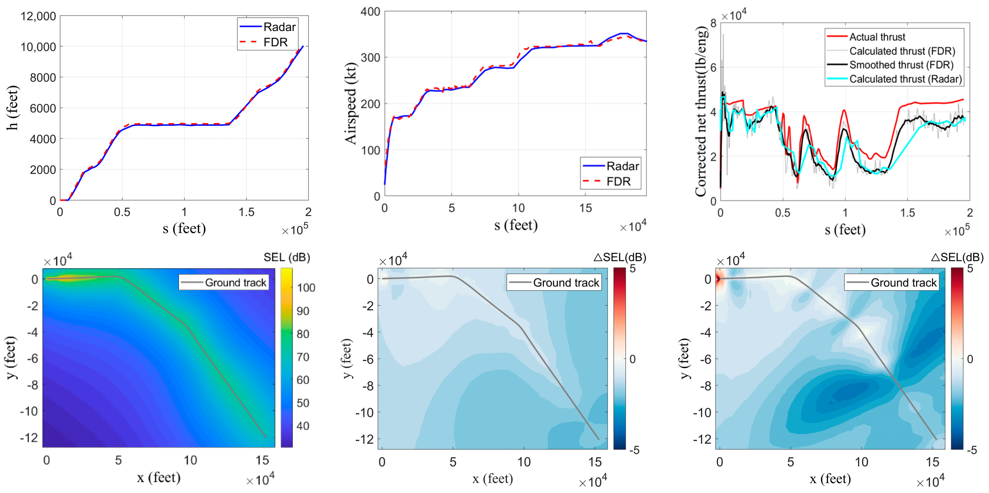
Appendix C.2. Noise Impact Incurred by A330-343 Aircraft Flying along Two Approach Routes

Mirroring Section 4.2.1, we here compare the noise impact induced by two A330-343 aircraft approaching HKIA, with a special focus on those densely populated areas (namely D2, D3, and D4) that are located beneath the flight corridors. The two flights are selected for their rather different flightpaths, so as to highlight how the latter may alter the noise footprint on the ground. More precisely, the first aircraft (flight AA2) approaches the 25L runway via a higher altitude route, while the second one (flight AA3) flies towards the 25R runway at a lower altitude. These differences hold to a certain point, after which both aircraft adopt a similar flightpath, following the Continuous Descent Approach protocol enforced in Hong Kong. Figure A8 depicts the ground track and flight profile of both flights.
Figure A8. A330 aircraft approaching HKIA. Flights AA2 and AA3 respective routes (left: ground track, center: flight profile) and corresponding ground observers (dynamic grid, right).
Aerospace 08 00264 g0a8
Figure A9 depicts the SEL contours incurred by both flight AA2 (left) and flight AA3 (center), along with their difference (right). The densely populated D3 district which is sandwiched between 25L and 25R routes sees its northwestern part impacted more importantly by flight AA3 (with noise levels exceeding AA2 ones by about 10.6 dB, see Figure A10), while the opposite occurs in the southeastern part (with an excess noise by flight AA2 of up to 7.8 dB). Given the distribution of residents in the D3 district (whose central and southern areas are more populated, see Figure 8), flight AA2 (lower altitude) appears to be less environmentally friendly than its AA3 counterpart (higher altitude). This observation also holds for the four times denser D2 district, which is flown over directly by flight AA2 whose noise impact exceeds the AA3 one by about 9.1 dB. Finally, both flights impact equally the D4 district, each incurring a noise excess of 1–2 dB underneath its respective route. To sum up, flight AA2 appears to be less environmentally friendly for these densely populated districts, thereby revealing that the 25R approach route should be given priority whenever the conditions permit (operational, meteorological, etc.). Notably, all these observations are fully consistent with the ones recorded for Boeing aircraft (cf. Section 4.2.1).
Figure A9. A330 aircraft approaching HKIA. Noise impact (SEL) generated by flight AA2 (left) and AA3 (center) over Hong Kong city, along with difference (∆SEL) between both results (as obtained by subtracting the former from the latter, right).
Aerospace 08 00264 g0a9
Figure A10. Difference in SEL (∆SEL) between flights AA2 and AA3 (closer view).
Aerospace 08 00264 g0a10

Appendix C.3. Specific Effect of the Bank Angle on the Various Routes and Aircraft

This section further illustrates the sensitivity of the noise prediction towards the bank angle (i.e., engines installation) effect, thereby extending the investigation conducted in Section 4.3.1. Here, we perform the noise prediction for alternatives flights, with the bank angle being either incorporated or neglected in the SEL evaluation.
Focusing first on departure scenarios, we consider the flights AD1 (cf. Section 4.2.1), BD4, and BD5 (cf. Appendix C.1) departing from HKIA. Similar to what happened for flight AD2 (cf. Section 4.3.1), when the aircraft performs a banked turn, most of the observers located on the same (resp. opposite) side of the turn experience less (resp. more) noise impacts (see Figure A11). The opposite nevertheless holds for those observers that are located very close to the ground track. All the previous observations derive logically from the relative depression angle perceived by each observer (see Section 2.3.2). This being said, the bank effect on the SEL levels appears to be fairly subtle, with differences of less than 0.4 dB overall (see Figure A11).
Figure A11. Various aircraft departing from HKIA. Difference in the noise impact (SEL) generated by flights AD1 (left), BD4 (center) and BD5 (right), due to the incorporation of bank angle effect.
Aerospace 08 00264 g0a11
Focusing then on approach scenarios, we repeat the noise prediction associated with flights AA3 (cf. Appendix C.2), BA1 and BA2 (cf. Section 4.2.1). Here too, the impact of the bank angle is rather modest, with no more than 0.5dB differences overall (see Figure A12). These differences are again positive or negative, depending on how each observer perceives the relative depression angle.
Figure A12. Various aircraft approaching HKIA. Difference in the noise impact (SEL) generated by flights AA3 (left), BA1 (center) and BA2 (right), due to the incorporation of bank angle effect.
Aerospace 08 00264 g0a12
All the above observations, which are fully consistent with those obtained in Section 4.3.1, further confirm that the noise impact is not that sensitive to the bank effect of turning flight segments. Even though of secondary importance, this effect however helps the noise prediction to better reflect real-life aircraft operations.

References

  1. International Civil Aviation Organisation (ICAO). Environmental Report 2010. Available online: https://www.icao.int/environmental-protection/Documents/Publications/ENV_Report_2010.pdf (accessed on 7 September 2021).
  2. Baudin, C.; Lefèvre, M.; Champelovier, P.; Lambert, J.; Laumon, B.; Evrard, A.-S. Aircraft Noise and Psychological Ill-Health: The Results of a Cross-Sectional Study in France. Int. J. Environ. Res. Public Health 2018, 15, 1642. [Google Scholar] [CrossRef] [PubMed] [Green Version]
  3. Peters, J.L.; Zevitas, C.D.; Redline, S.; Hastings, A.; Sizov, N.; Hart, J.E.; Levy, J.I.; Roof, C.J.; Wellenius, G.A. Aviation Noise and Cardiovascular Health in the United States: A Review of the Evidence and Recommendations for Research Direction. Curr. Epidemiol. Rep. 2018, 5, 140–152. [Google Scholar] [CrossRef]
  4. Nassur, A.-M.; Léger, D.; Lefèvre, M.; Elbaz, M.; Mietlicki, F.; Nguyen, P.; Ribeiro, C.; Sineau, M.; Laumon, B.; Evrard, A.-S. Effects of Aircraft Noise Exposure on Heart Rate during Sleep in the Population Living Near Airports. Int. J. Environ. Res. Public Health 2019, 16, 269. [Google Scholar] [CrossRef] [Green Version]
  5. European Aviation Environmental Report 2019; European Environment Agency; European Aviation Safety Agency; Eurocontrol: Copenhagen, Denmark, 2019. [CrossRef]
  6. Thomas, C.; Hume, K.; Hooper, P. Aircraft Noise, Airport Growth and Regional Development. In Proceedings of the 10th AIAA/CEAS Aeroacoustics Conference, Manchester, UK, 10–12 May 2004; p. 2806. [Google Scholar] [CrossRef]
  7. Upham, P.; Thomas, C.; Gillingwater, D.; Raper, D. Environmental capacity and airport operations: Current issues and future prospects. J. Air Transp. Manag. 2003, 9, 145–151. [Google Scholar] [CrossRef]
  8. Zaporozhets, O.; Tokarev, V.; Attenborough, K.; Miller, N.P. Aircraft Noise Assessment, Prediction and Control. Noise Control. Eng. J. 2012, 60, 222. [Google Scholar] [CrossRef]
  9. Port Authority of New York and New Jersey. Airport Traffic Report. 2019. Available online: https://www.panynj.gov/airports/en/statistics-general-info.html (accessed on 7 September 2021).
  10. Wei, N.; Zhu, F.; ChaoGao, Z. Research on Airport Noise Prediction Method Based on Noise Model INM. In Proceedings of the 2020 12th International Conference on Machine Learning and Computing, Shenzhen, China, 15–17 February 2020; pp. 489–494. [Google Scholar] [CrossRef]
  11. Ziyao, X.; Xisheng, H. A Study on the Legislation Issues of Airport Noise Abatement in China. J. Beijing Univ. Aeronaut. Astronaut. Soc. Sci. Ed. 2011, 24, 38. [Google Scholar] [CrossRef]
  12. Centre for Aviation. China Becomes the Largest Aviation Market in the World. 2020. Available online: https://centreforaviation.com/analysis/reports/china-becomes-the-largest-aviation-market-in-the-world-521779 (accessed on 7 September 2021).
  13. Law, C.K.; Fung, M.; Law, J.; Tse, D.; Chan, K.Y. HKIA’s Third Runway—The Key for Enhancing Hong Kong’s Aviation Position. Aviat. Policy Res. Cent. Novemb. 2007, 28. Available online: https://citeseerx.ist.psu.edu/viewdoc/download?doi=10.1.1.493.3575&rep=rep1&type=pdf (accessed on 7 September 2021).
  14. Leylekian, L.; Lebrun, M.; Lempereur, P. An Overview of Aircraft Noise Reduction Technologies. AerospaceLab 2014, 1–15. [Google Scholar] [CrossRef]
  15. Alam, S.; Nguyen, M.H.; Abbass, H.; Lokan, C.; Ellejmi, M.; Kirby, S. Multi-Aircraft Dynamic Continuous Descent Approach Methodology for Low-Noise and Emission Guidance. J. Aircr. 2011, 48, 1225–1237. [Google Scholar] [CrossRef]
  16. Clarke, J.-P.B.; Ho, N.T.; Ren, L.; Brown, J.A.; Elmer, K.R.; Tong, K.-O.; Wat, J.K. Continuous Descent Approach: Design and Flight Test for Louisville International Airport. J. Aircr. 2004, 41, 1054–1066. [Google Scholar] [CrossRef]
  17. Alam, S.; Nguyen, M.H.; Abbass, H.A.; Lokan, C.; Ellejmi, M.; Kirby, S. A dynamic continuous descent approach methodology for low noise and emission. In Proceedings of the 29th Digital Avionics Systems Conference, Salt Lake City, UT, USA, 3–7 October 2010; p. 1-E. [Google Scholar] [CrossRef]
  18. Bertsch, L.; Dobrzynski, W.; Guérin, S. Tool Development for Low-Noise Aircraft Design. J. Aircr. 2010, 47, 694–699. [Google Scholar] [CrossRef]
  19. Molin, N.; Piet, J.-F.; Chow, L.C.; Smith, M.; Dobrzynski, W.; Seror, C. Prediction of Low Noise Aircraft Landing Gears and Comparison with Test Results. In Proceedings of the 12th AIAA/CEAS Aeroacoustics Conference, Cambridge, MA, USA, 8–10 May 2006; p. 2623. [Google Scholar] [CrossRef]
  20. Bertsch, L.; Heinze, W.; Lummer, M. Application of an Aircraft Design-To-Noise Simulation Process. In Proceedings of the 14th AIAA Aviation Technology, Integration, and Operations Conference, Atlanta, GA, USA, 16–20 June 2014; p. 2169. [Google Scholar] [CrossRef]
  21. Nero, G.; Black, J.A. A critical examination of an airport noise mitigation scheme and an aircraft noise charge: The case of capacity expansion and externalities at Sydney (Kingsford Smith) airport. Transp. Res. Part D Transp. Environ. 2000, 5, 433–461. [Google Scholar] [CrossRef]
  22. Arafa, M.H.; Osman, T.; Abdel-Latif, I.A. Noise assessment and mitigation schemes for Hurghada airport. Appl. Acoust. 2007, 68, 1373–1385. [Google Scholar] [CrossRef]
  23. Koster, R. Using NOMOS Measurements to Assess Improvements of ECAC Doc. 29 Aircraft Noise Calculations; Delft University of Technology: Delft, The Netherlands, 2020; Available online: http://resolver.tudelft.nl/uuid:a8ba2f3c-7289-4aff-ad8a-5b358cd4ffbe (accessed on 7 September 2021).
  24. Raimbault, M.; Dubois, D. Urban soundscapes: Experiences and knowledge. Cities 2005, 22, 339–350. [Google Scholar] [CrossRef]
  25. Filippone, A. Aircraft noise prediction. Prog. Aerosp. Sci. 2014, 68, 27–63. [Google Scholar] [CrossRef]
  26. Bertsch, L.; Schäffer, B.; Guérin, S. Uncertainty Analysis for Parametric Aircraft System Noise Prediction. J. Aircr. 2019, 56, 529–544. [Google Scholar] [CrossRef]
  27. Pietrzko, S.; Rudolf, B. FLULA-Swiss Aircraft Noise Prediction Program. Proc. Acoust. 2002, 13–15. Available online: https://www.dora.lib4ri.ch/empa/islandora/object/empa:11080 (accessed on 7 September 2021).
  28. Ollerhead, J.B. The CAA Aircraft Noise Contour Model: ANCON Version 1. Civ. Aviat. Auth. Dep. Transp. 1992. Available online: https://publicapps.caa.co.uk/docs/33/ERCD9120.PDF (accessed on 7 September 2021).
  29. Ollerhead, J.; Sharp, B. MAGENTA-assessments of future aircraft noise policy options. Air Space Eur. 2001, 3, 247–249. [Google Scholar] [CrossRef]
  30. Roof, C.; Hansen, A.; Fleming, G.; Thrasher, T.; Nguyen, A.; Hall, C.; Dinges, E.; Grandi, F.; Kim, B.; Usdrowski, S. Aviation Environmental Design Tool (AEDT) System Architecture. Fed. Aviat. Adm. Off. Environ. Energy 2007. Available online: https://rosap.ntl.bts.gov/view/dot/12254 (accessed on 7 September 2021).
  31. Wunderli, J.M.; Zellmann, C.; Köpfli, M.; Habermacher, M. sonAIR—A GIS-Integrated Spectral Aircraft Noise Simulation Tool for Single Flight Prediction and Noise Mapping. Acta Acust. United Acust. 2018, 104, 440–451. [Google Scholar] [CrossRef]
  32. Bertsch, L.; Sébastien, G.; Looye, G.; Pott Pollenske, M. The Parametric Aircraft Noise Analysis Module-Status Overview and Recent Applications. In Proceedings of the 17th AIAA/CEAS Aeroacoustics Conference, Portland, OR, USA, 5–8 June 2011; p. 2855. [Google Scholar] [CrossRef] [Green Version]
  33. Jäger, D.; Zellmann, C.; Schlatter, F.; Wunderli, J.M. Validation of the sonAIR aircraft noise simulation model. Noise Mapp. 2021, 8, 95–107. [Google Scholar] [CrossRef]
  34. Malbéqui, P.; Rozenberg, Y.; Bulté, J. Aircraft Noise Prediction in the IESTA Program. In Proceedings of the 3rd European Conference for Aerospace Sciences, Versailles, France, 6–9 July 2009; Available online: https://www.onera.fr/sites/default/files/Departements-scientifiques/DCPS/AircraftnoisepredictionintheIESTAprogram.pdf (accessed on 7 September 2021).
  35. Lopes, L.; Burley, C. Design of the next Generation Aircraft Noise Prediction Program: ANOPP2. In Proceedings of the 17th AIAA/CEAS Aeroacoustics Conference, Portland, OR, USA, 5–8 June 2011; p. 2854. [Google Scholar] [CrossRef] [Green Version]
  36. Tuinstra, M. A Fast Atmospheric Sound Propagation Model for Aircraft Noise Prediction. Int. J. Aeroacoustics 2014, 13, 337–361. [Google Scholar] [CrossRef]
  37. Boeker, E.R.; Dinges, E.; He, B.; Fleming, G.; Roof, C.J.; Gerbi, P.J.; Rapoza, A.S.; Hermann, J.; United States. Federal Aviation Administration; Office of Environment and Energy. Integrated Noise Model (INM) Version 7.0 Technical Manual. 2008. Available online: https://rosap.ntl.bts.gov/view/dot/12188 (accessed on 7 September 2021).
  38. Mato, R.R.; Mufuruki, T. Noise pollution associated with the operation of the Dar es Salaam International Airport. Transp. Res. Part D Transp. Environ. 1999, 4, 81–89. [Google Scholar] [CrossRef]
  39. Eriksson, C.; Bluhm, G.; Hilding, A.; Östenson, C.-G.; Pershagen, G. Aircraft noise and incidence of hypertension—Gender specific effects. Environ. Res. 2010, 110, 764–772. [Google Scholar] [CrossRef]
  40. Babisch, W.; Pershagen, G.; Selander, J.; Houthuijs, D.; Breugelmans, O.; Cadum, E.; Vigna-Taglianti, F.; Katsouyanni, K.; Haralabidis, A.S.; Dimakopoulou, K.; et al. Noise annoyance—A modifier of the association between noise level and cardiovascular health? Sci. Total. Environ. 2013, 452–453, 50–57. [Google Scholar] [CrossRef]
  41. Ignaccolo, M. Environmental capacity: Noise pollution at Catania-Fontanarossa international airport. J. Air Transp. Manag. 2000, 6, 191–199. [Google Scholar] [CrossRef]
  42. El Fadel, M.; Chahine, M.; Baaj, M.; Mezher, T. Managing Noise Emission Impacts of Airport Traffic. INTER-NOISE NOISE-CON Congr. Conf. Proc. 2000, 2000, 1395–1399. Available online: http://www.conforg.fr/internoise2000/cdrom/data/articles/000863.pdf (accessed on 7 September 2021).
  43. Hebly, S.J.; Visser, H.G. Advanced noise abatement departure procedures: Custom-optimised departure profiles. Aeronaut. J. 2015, 119, 647–661. [Google Scholar] [CrossRef]
  44. Clarke, J.-P.; Bennett, D.; Elmer, K.; Firth, J.; Hilb, R.; Ho, N.; Johnson, S.; Lau, S.; Ren, L.; Senechal, D. Development, Design, and Flight Test Evaluation of a Continuous Descent Approach Procedure for Nighttime Operation at Louisville International Airport. Partnership for Air Transportation Noise and Emissions Reduction. 2006. Available online: https://rosap.ntl.bts.gov/view/dot/28416 (accessed on 7 September 2021).
  45. Kim, D.; Lyu, Y.; Liem, R.P. Flight Profile Optimization for Noise Abatement and Fuel Efficiency during Departure and Arrival of an Aircraft. AIAA Aviation 2019 Forum 2019, 3622. [Google Scholar] [CrossRef]
  46. Wijnen, R.; Visser, H. Optimal departure trajectories with respect to sleep disturbance. Aerosp. Sci. Technol. 2003, 7, 81–91. [Google Scholar] [CrossRef]
  47. U.S. Department of Transportation. NextGen Annual Report. Available online: https://www.faa.gov/nextgen/media/NextGenAnnualReport-FiscalYear2020.pdf (accessed on 7 September 2021).
  48. Environmental Protection Agency, Ireland. Guidance Note for Strategic Noise Mapping For the Environmental Noise Regulations 2006. Available online: https://www.epa.ie/publications/monitoring--assessment/noise/EPA-Guidance-Note-for-Strategic-Noise-Mapping-(version-2).pdf (accessed on 7 September 2021).
  49. Report on Standard Method of Computing Noise Contours around Civil Airports. Eur. Civ. Aviat. Conf. 2016, 2. Available online: https://www.ecac-ceac.org/images/documents/ECAC-Doc_29_4th_edition_Dec_2016_Volume_2.pdf (accessed on 7 September 2021).
  50. Kephalopoulos, S.; Paviotti, M.; Anfosso-Lédée, F. Common Noise Assessment Methods in Europe (CNOSSOS-EU). Publ. Off. Eur. Union 2012, 180. [Google Scholar] [CrossRef]
  51. Civil Aviation Authority. Strategic Noise Maps for Heathrow Airport 2016. 2018. Available online: https://publicapps.caa.co.uk/docs/33/MappingHeathrow.pdf (accessed on 7 September 2021).
  52. Vogiatzis, K.; Remy, N. Strategic Noise Mapping of Herakleion: The Aircraft Noise Impact as a factor of the Int. Airport relocation. Noise Mapp. 2014, 1. [Google Scholar] [CrossRef]
  53. Procedure for the Calculation of Airplane Noise in the Vicinity of Airports. Soc. Automot. Eng. Comm. A-21 2012. [CrossRef]
  54. Federal Aviation Administration. Fundamentals of Noise and Sound. 2020. Available online: https://www.faa.gov/regulations_policies/policy_guidance/noise/basics/ (accessed on 7 September 2021).
  55. International Civil Aviation Organization. Recommended Method for Computing Noise Contours Around Airports. 2008. Available online: https://global.ihs.com/doc_detail.cfm?document_name=ICAO9911&item_s_key=00520247 (accessed on 7 September 2021).
  56. Vos, E.; Groenendijk, J.; Do, M.T.; Tyre and Road Surface Optimisation for Skid Resistance and Further Effects. D05 Report on Analysis and Findings of Previous Skid Resistance Harmonisation Research Projects. 2009. Available online: https://trimis.ec.europa.eu/sites/default/files/project/documents/20120406_001647_43476_TYROSAFEFINALSummaryReport.pdf (accessed on 7 September 2021).
  57. Matamoros Cid, I. Modelling Flexible Thrust Performance for Trajectory Prediction Applications in Air Traffic Management; Universitat Politècnica de Catalunya: Barcelona, Spain, 2015; Available online: http://hdl.handle.net/2117/85938 (accessed on 7 September 2021).
  58. Thacker, W.C. A brief review of techniques for generating irregular computational grids. Int. J. Numer. Methods Eng. 1980, 15, 1335–1341. [Google Scholar] [CrossRef]
  59. Settari, A.; Aziz, K. Use of Irregular Grid in Reservoir Simulation. Soc. Pet. Eng. J. 1972, 12, 103–114. [Google Scholar] [CrossRef]
  60. Standard Values of Atmospheric Absorption as a Function of Temperature and Humidity. Soc. Automot. Eng. Comm. A-21 1975. [CrossRef]
  61. Rickley, E.J.; Fleming, G.G.; Roof, C.J. Simplified procedure for computing the absorption of sound by the atmosphere. Noise Control. Eng. J. 2007, 55, 482. [Google Scholar] [CrossRef]
  62. Report on Standard Method of Computing Noise Contours around Civil Airports. Eur. Civ. Aviat. Conf. 2016, 3. Available online: https://www.ecac-ceac.org/images/documents/ECAC-Doc_29_4th_edition_Dec_2016_Volume_3_Part_1.pdf (accessed on 7 September 2021).
  63. European Union Aviation Safety Agency. Type Certificate Data Sheets (TCDS). 2021. Available online: https://www.easa.europa.eu/document-library/type-certificates (accessed on 7 September 2021).
  64. International Standards and Recommended Practices, Environmental Protection, Annex 16. Int. Civ. Aviat. Organ. 2008, 1. Available online: https://www.caat.or.th/wp-content/uploads/2016/04/AN16_V1_cons.pdf (accessed on 7 September 2021).
  65. HaoLei, L. Research on the Evaluation Method of Aircraft Airworthiness Lateral Noise; Civil Aviation University of China: Tianjin, China, 2018. [Google Scholar] [CrossRef]
  66. Hong Kong Civil Aviation Department. Aircraft Noise Management. 2021. Available online: https://www.cad.gov.hk/english/ac_noise.html (accessed on 7 September 2021).
  67. Albéri, M.; Baldoncini, M.; Bottardi, C.; Chiarelli, E.; Fiorentini, G.; Raptis, K.G.C.; Realini, E.; Reguzzoni, M.; Rossi, L.; Sampietro, D.; et al. Accuracy of Flight Altitude Measured with Low-Cost GNSS, Radar and Barometer Sensors: Implications for Airborne Radiometric Surveys. Sensors 2017, 17, 1889. [Google Scholar] [CrossRef] [PubMed] [Green Version]
  68. Manolakis, D.; Lefas, C.; Rekkas, C. Computation of aircraft geometric height under radar surveillance. IEEE Trans. Aerosp. Electron. Syst. 1992, 28, 241–248. [Google Scholar] [CrossRef]
  69. Poles, D.; Nuic, A.; Mouillet, V. Advanced Aircraft Performance Modeling for ATM: Analysis of BADA Model Capabilities. In Proceedings of the 29th Digital Avionics Systems Conference, Salt Lake City, UT, USA, 3–7 October 2010; p. 1-D. [Google Scholar] [CrossRef]
  70. Sherry, L.; Neyshabouri, S. Estimating Takeoff Thrust from Surveillance Track Data. Transportation Research Board Annual Meeting. 2014. Available online: https://catsr.vse.gmu.edu/pubs/EstTakeoffThrustTrackData%5B4%5DTRB.pdf (accessed on 7 September 2021).
  71. Nuic, A. User Manual for the Base of Aircraft Data (BADA) Revision 3.10. Atmosphere 2010, 2010, 1. Available online: https://www.eurocontrol.int/sites/default/files/library/022_BADA_User_Manual.pdf (accessed on 7 September 2021).
  72. Poulain, K. Numerical Propagation of Aircraft En Route Noise; The Pennsylvania State University: University Park, PA, USA, 2011; Available online: https://etda.libraries.psu.edu/catalog/12491 (accessed on 7 September 2021).
  73. Heath, S.; McAninch, G. Propagation Effects of Wind and Temperture on Acoustic Ground Contour Levels. In Proceedings of the 44th AIAA Aerospace Sciences Meeting and Exhibit, Reno, NV, USA, 9–12 January 2006; p. 411. [Google Scholar] [CrossRef] [Green Version]
  74. Arntzen, M.; Hordijk, M.; Simons, D.G. Including Atmospheric Propagation Effects in Aircraft Take-off Noise Modeling. In Proceedings of the 43rd International Congress on Noise Control Engineering, Melbourne, Australia, 16–19 November 2014; Available online: https://acoustics.asn.au/conference_proceedings/INTERNOISE2014/papers/p307.pdf (accessed on 7 September 2021).
  75. Dikshit, P.; Crossley, W. Airport Noise Model Suitable for Fleet-Level Studies. In Proceedings of the 9th AIAA Aviation Technology, Integration, and Operations Conference (ATIO) and Aircraft Noise and Emissions Reduction Symposium (ANERS), Hilton Head, SC, USA, 21–23 September 2009; p. 6937. [Google Scholar] [CrossRef]
Figure 1. Aircraft noise prediction methodology, as built-up from the baseline approach [49] (in black) whereas incorporating specific addendums (in red).
Aerospace 08 00264 g001
Figure 2. Engine installation effects on aircraft noise directivity. Noise level correction (dB) as a function of depression angle (deg).
Aerospace 08 00264 g002
Figure 3. Meteorological effects on aircraft noise intensity. Impedance adjustment as a function of the atmospheric pressure and temperature.
Aerospace 08 00264 g003
Figure 4. Meteorological effects on aircraft noise intensity. Absorption adjustment (difference in SEL with respect to that of a standard atmosphere).
Aerospace 08 00264 g004
Figure 5. Noise contour map (top) and corresponding error (bottom) for JETFDC (left), JETWDC (center), PROPDC (right) cases.
Aerospace 08 00264 g005
Figure 6. Noise contour map (top) and corresponding error (bottom) for JETFAC (left), JETWAC (center), PROPAC (right) cases.
Aerospace 08 00264 g006
Figure 7. Reference measurement points in noise certification tests.
Aerospace 08 00264 g007
Figure 8. Noise impact by aircraft operation around Hong Kong. Left: Distribution of Hong Kong’s population (2020 year). Center: flightpaths of aircraft flying from/to HKIA whereas passing over densely populated districts in Hong Kong (D1 to D7). Right: A330 aircraft departing from HKIA following a standard departure route.
Aerospace 08 00264 g008
Figure 9. A330 aircraft departing from HKIA. Flights AD1 and AD2 respective routes (left: ground track, center: flight profile) and corresponding ground observers (dynamic grid, right).
Aerospace 08 00264 g009
Figure 10. A330 aircraft departing from HKIA. Noise impact (SEL) generated by flight AD1 (left) and AD2 (right) over Hong Kong city.
Aerospace 08 00264 g010
Figure 11. Difference in the noise impact (∆SEL) by flights AD1 and AD2 (as obtained by subtracting the former from the latter), with a closer view provided on the right side.
Aerospace 08 00264 g011
Figure 12. Power settings (engine thrust) evolution of flights AD1 and AD2.
Aerospace 08 00264 g012
Figure 13. B777 aircraft approaching HKIA. Flights BA1 and BA2 respective routes (left: ground track, center: flight profile) and corresponding ground observers (dynamic grid, right).
Aerospace 08 00264 g013
Figure 14. B777 aircraft approaching HKIA. Noise impact (SEL) generated by flight BA1 (left) and BA2 (right) over Hong Kong city.
Aerospace 08 00264 g014
Figure 15. Difference in the noise impact (∆SEL) by flights BA1 and BA2 (as obtained by subtracting the former from the latter), with a closer view provided on right side.
Aerospace 08 00264 g015
Figure 16. A330 aircraft departing from HKIA. Aircraft noise impact on the ground, as depicted in terms of SEL for cases AD3, AD4, AD5, AD6 (from left to right, respectively).
Aerospace 08 00264 g016
Figure 17. Effect of the atmospheric properties on the aircraft noise impact. Differences in SEL induced by a variation in temperature, as obtained for a given relative humidity (left: AD4—AD3, right: AD6—AD5).
Aerospace 08 00264 g017
Figure 18. Effect of the atmospheric properties on the aircraft noise impact. Differences in SEL induced by a variation in relative humidity, as obtained for a given temperature (left: AD5—AD3, right: AD6—AD4).
Aerospace 08 00264 g018
Figure 19. Effect of the atmospheric properties on the aircraft noise impact. Differences in SEL induced by a variation in both temperature and relative humidity (AD6—AD3).
Aerospace 08 00264 g019
Figure 20. A330 and (virtual) B777 aircraft departing from HKIA. Noise levels (SEL) generated by flight AD2 (left) and BD1 (center) over Hong Kong city, along with their difference (obtained by subtracting the former from the latter, right).
Aerospace 08 00264 g020
Figure 21. A330 and B777 aircraft noise impact (SEL) as recorded for various power settings (corrected thrust) and propagation distances. Excerpted from NPD database.
Aerospace 08 00264 g021
Figure 22. B777 and (virtual) A330 aircraft approaching HKIA. Noise levels (SEL) generated by flight BA1 (left) and AA1 (center), along with their difference (obtained by subtracting the former from the latter, right).
Aerospace 08 00264 g022
Figure 23. A330 aircraft departing from HKIA. Noise impact (SEL) generated by flight AD2 with (left) and without (center) the incorporation of the installation effect (bank angle), along with the difference between both results (obtained by subtracting the former from the latter, right).
Aerospace 08 00264 g023
Figure 24. A330 aircraft departing from HKIA. Impact of the flightpath extension, as revealed by comparing flight AD1-ext to AD1. Left: respective routes and ground observers. Center: history of the ground noise impact by the AD1-ext flight, plotted as an averaged (over all observers) and cumulative (over all flight segments) measure. Right: Differences between the ground noise levels recorded for AD1-ext and AD1 flights.
Aerospace 08 00264 g024
Figure 25. Flight profiles of B777 and A330 aircraft departing from HKIA (grey curves), with two pairs of flights selected (namely, BD2 and BD3, AD7 and AD8).
Aerospace 08 00264 g025
Figure 26. B777 aircraft departing from HKIA (flight BD2). Top: Comparison between the flight profile (left), airspeed (center), calculated and actual thrust (right) inferred from the FDR and radar data. Bottom: Noise contour map, as obtained using FDR data and actual thrust (left). Error entailed by an approximation of the thrust (center: smooth calculated thrust) plus the trajectory estimation (right: radar data, calculated thrust).
Aerospace 08 00264 g026
Figure 27. B777 aircraft departing from HKIA (flight BD3). Top: Comparison between the flight profile (left), airspeed (center), calculated and actual thrust (right) inferred from the FDR and radar data. Bottom: Noise contour map, as obtained using FDR data and actual thrust (left). Error entailed by an approximation of the thrust (center: smooth calculated thrust) plus the trajectory estimation (right: radar data, calculated thrust).
Aerospace 08 00264 g027
Figure 28. A330 aircraft departing from HKIA (flight AD7). Top: Comparison between the flight profile (left), airspeed (center), calculated and actual thrust (right) inferred from the FDR and radar data. Bottom: Noise contour map, as obtained using FDR data and actual thrust (left). Error entailed by an approximation of the thrust (center: smooth calculated thrust) plus the trajectory estimation (right: radar data, calculated thrust).
Aerospace 08 00264 g028
Figure 29. A330 aircraft departing from HKIA (flight AD8). Top: Comparison between the flight profile (left), airspeed (center), calculated and actual thrust (right) inferred from the FDR and radar data. Bottom: Noise contour map, as obtained using FDR data and actual thrust (left). Error entailed by an approximation of the thrust (center: smooth calculated thrust) plus the trajectory estimation (right: radar data, calculated thrust).
Aerospace 08 00264 g029
Table 1. Errors between the calculated noise levels and the reference results.
Reference Case δ max   ( dB ) δ RMS   ( dB )
JETFAC0.01250.00135
JETFAS0.01250.00149
JETFDC0.01250.00237
JETFDS0.01250.00160
JETWAC0.01250.00183
JETWAS0.01250.00179
JETWDC0.01250.00215
JETWDS0.01250.00157
PROPAC0.01000.00218
PROPAS0.00160.00162
PROPDC0.02000.00423
PROPDS0.01240.00159
Table 2. Noise levels for B737-800 and A320-211 aircraft at three certification points, as measured and calculated (in EPNdB) with associated errors (in percentage).
ApproachLateralFlyover
A320-211B737-800A320-211B737-800A320-211B737-800
Measurement96.1096.3093.7093.9087.4086.40
Present study96.3294.8094.4194.7194.4094.00
Error0.2291.5580.7580.8638.0098.796
Table 3. Yearly extrema in atmospheric conditions recorded in Hong Kong (sea level pressure) and meteorological scenarios considered for the four flights.
Temperature (°C)
735
Relative
humidity (%)
13AD3AD4
100AD5AD6
Publisher’s Note: MDPI stays neutral with regard to jurisdictional claims in published maps and institutional affiliations.

