Aircraft Trajectory Clustering in Terminal Airspace Based on Deep Autoencoder and Gaussian Mixture Model

Abstract

The aircraft trajectory clustering analysis in the terminal airspace is conducive to determining the representative route structure of the arrival and departure trajectory and extracting their typical patterns, which is important for air traffic management such as airspace structure optimization, trajectory planning, and trajectory prediction. However, the current clustering methods perform poorly due to the large flight traffic, high density, and complex airspace structure in the terminal airspace. In recent years, the continuous development of Deep Learning has demonstrated its powerful ability to extract internal potential features of large dataset. Therefore, this paper mainly tries a deep trajectory clustering method based on deep autoencoder (DAE). To this end, this paper proposes a trajectory clustering method based on deep autoencoder (DAE) and Gaussian mixture model (GMM) to mine the prevailing traffic flow patterns in the terminal airspace. The DAE is trained to extract feature representations from historical high-dimensional trajectory data. Subsequently, the output of DAE is input into GMM for clustering. This paper takes the terminal airspace of Guangzhou Baiyun International Airport in China as a case to verify the proposed method. Through the direct visualization and dimensionality reduction visualization of the clustering results, it is found that the traffic flow patterns identified by the clustering method in this paper are intuitive and separable.

1. Introduction

The terminal airspace surrounding an airport has significant flight traffic, high density, and complex airspace structure. According to statistics released by Boeing, 60% of the world’s commercial aircraft accidents occurred during take-off, initial climb, approach, and landing stages, from 2007 to 2016, although these four stages only accounted for 6% of the total flight time, which posed a great threat to air transportation safety [1]. Therefore, the research and development of automated decision support tools mainly focus on the terminal area to help controllers with conflict detection and resolution, arrival and departure sequencing, aircraft abnormal behavior monitoring, and other air traffic management behaviors.

NextGen in the United States and SESAR in Europe have promoted the transformation of the current air traffic management mode to a new mode based on trajectory operation (TBO). This mode mainly uses 4D trajectory as the basic information for managing safety and capacity. Among them, the trajectory prediction process is a key component of TBO, and it relies on the precise clustering of aircraft trajectories [2]. The trajectory clustering algorithm can also be integrated into tools that support airspace design/management, complexity management, and so on. In addition, trajectory cluster analysis is an important step in trajectory planning, which is mainly to find out the prevailing traffic flow and to provide reference for terminal airspace trajectory planning. The trajectory planning can not only provide an effective path for conflict resolution, but also generate the corresponding 4D trajectory according to the optimized time generated by the arrival and departure schedule to ensure that the aircraft arrives at the designated location safely and on time, thereby reducing flight delays and improving operational efficiency. It can be seen that trajectory clustering is the foundation of many air traffic management tasks, and it is of great significance to the optimization of airspace structure, trajectory planning, abnormal trajectory detection, and trajectory prediction.

At present, many scholars have conducted a lot of research on trajectory clustering. Lee et al. [3] proposed a new trajectory clustering and grouping framework, which used a standard trajectory segmentation algorithm of minimum description length (MDL) to divide a trajectory into a set of line segments and then used a density-based line segment clustering algorithm to divide similar line segments into a cluster. Eckstein et al. [4] proposed an automatic flight trajectory classification method, which used K-Means clustering based on principal component analysis (PCA). Sabhnani et al. [5] extracted the traffic structure based on standard flows and critical points (conflict points and merging points), mainly used two methods of greedy trajectory clustering and ridge top detection to identify standard flows, and determined the intersection of two or more standard flows as the critical point. Rehm [6] only defined the similarity between the trajectories, including the pairwise similarity, the closed area between the trajectories, and the grid-based similarity, and discussed the advantages and disadvantages of using different similarity measures in the clustering process. Gariel et al. [7] proposed the longest common subsequence (LCS) clustering method based on turning point recognition, considering the trajectory characteristics of aircraft that usually fly directly and have fewer turns. Annoni et al. [8] used Fourier descriptors to describe the characteristics of the actual aircraft trajectories in the terminal area and clustered them. At the same time, they used kernel density estimation to classify the trajectory points to detect abnormal traffic conditions. Wang et al. [9] established a similarity measurement model between trajectories based on the inverse comparison of corresponding trajectory points and applied the hierarchical clustering method. Since most of the existing flow recognition algorithms rely only on spatial clustering without considering the time dimension, Enriquez et al. [10] proposed a spectral clustering framework to solve this shortcoming producing robust results. Ayhan et al. [2] proposed an aircraft trajectory clustering framework based on segmentation, clustering, and merging, which divided and clustered the trajectory points according to the three main flight stages of the climb, cruise, and descent, and then merged to obtain the clustering results of the entire trajectory. Xu et al. [11] used the normal distance of the trajectory point as the similarity measurement index and used the K-medoids clustering algorithm to cluster, which effectively solved the mismatch problem in trajectory point selection caused by the difference in aircraft speed. Mcfadyen et al. [12] proposed a statistical-based clustering method for aircraft trajectories, which used the iterative K-medoids method to cluster the trajectories based on circular distribution statistics to resample the angle data. Pan et al. [13] constructed a multi-factor Hausdorff distance as a similarity measure and proposed a density-based multi-dimensional trajectory clustering algorithm. Eerland et al. [14] clustered the trajectory data and generated a probability model for each cluster, and weighted the trajectory based on the probability model to generate a representative trajectory. Mahboubi et al. [15] adopted a method based on trajectory turning point recognition and clustering. This method works well when the heading angular velocity data are not too noisy, but the effect is poor when there is noise in the actual data.

Basora et al. [16] proposed a new Hierarchical Density-Based Spatial Clustering of Applications with Noise (HDBSCAN) air traffic flow analysis framework, managing different densities with a single input parameter. Liu et al. [17] obtained typical trajectories through the three-step framework clustering in [4] to analyze the reasons for inefficient operation. Gallego et al. [18] discussed the progress of density-based clustering techniques, such as OPTICS and HDBSCAN*, and evaluated them quantitatively and qualitatively. In addition, they proposed a hierarchical clustering algorithm based on cyclic DBSCAN* (RDBSCAN*). Based on the principle of information bottleneck (IB), the clustering method does not need to predefine the number of clusters and the distance measurement between trajectories, which is effective for trajectory data. Therefore, Guo et al. [19] proposed an interactive visual analysis prototype IBVis for trajectory data. Wang et al. [20] combined LOF algorithm, K-Means clustering algorithm based on time window segmentation, and hierarchical clustering algorithm, and proposed a time window segmentation algorithm based on trajectory point features. Barratt et al. [21] used K-Means to cluster aircraft trajectories, combined with the Gaussian mixture model to learn the trajectory probability generation model of the airport terminal area. Locality Sensitive Hashing (LSH) is a commonly used data mining technique for finding similar items in high-dimensional data, so it is suitable for grouping similar flight paths in trajectory data. Given this, Tran et al. [22] proposed an adaptive LSH algorithm suitable for duplicate document detection, which clusters the nearest trajectories by representing the trajectory as a packet of words commonly used in text mining. Given that Deep Learning has the potential of using deep clustering techniques to discover hidden and more complex relationships in low-dimensional latent spaces, Olive et al. [23] explored the application of deep trajectory clustering based on autoencoders to the problem of flow identification. Samantha et al. [24] applied the HDBSCAN algorithm on the basis of a weighted Euclidean distance function to improve the identification of terminal airspace air traffic flows. To improve the accuracy of the anomaly detection models from surveillance data, Deshmukh et al. embedded a data preprocessing step that involves clustering of the source dataset using DBSCAN [25] and HDBSAN [26] algorithm. Olive et al. [27] proposed an algorithm that computes a clustering on subsets of significant points of trajectories while keeping a dependency tree of their temporal chaining and then associates trajectories to root-to-leaf paths in the dependency tree based on the clusters they cross. Olive et al. [28] also combined a trajectory clustering method to identify air traffic flows within the considered airspace with a technique to detect anomalies in each flow. Mayara et al. [29] first performed a multi-layer clustering analysis to mine spatial and temporal trends in flight trajectory data for identification of traffic flow patterns. M. Conde Rocha Murca et al. [30] developed an air traffic flow characterization framework composed of three sequential modules. The first module uses DBSACN to learn typical patterns of operation from radar tracks [31]. Built on this knowledge, the second module uses random forests to identify non-conforming trajectories. Finally, the third module uses K-Means to extract recurrent modes of operation (operational patterns) from the outcomes of the second module. A. Bombelli et al. [32] proposed an approach that involves coarse clustering, outlier detection, fine clustering, and aggregate route construction. Coarse clustering is based on common origin, destination, and average cruise speed. Fine clustering, based on the Fréchet distance between pairs of trajectories, is applied to each coarse cluster to subdivide it, if appropriate. In summary, multiple trajectory clustering algorithms exist in the literature to cluster point-based data such as K-Means, OPTICS, DBSCAN, HDBSCAN, and hierarchical or spectral clustering. In addition, there are some studies that use clustering algorithms to cluster trajectory segments. In addition to clustering algorithms, some studies also focus on how to define an appropriate distance function between pairs of trajectory points such as Euclidean, LCSS, DTW, Hausdorff, or Fréchet. However, some clustering algorithms require the trajectories to have the same length. Aiming at the clustering problem of inconsistent trajectory sequence length, some researchers conduct equal time interval sampling on the original trajectory from the perspective of data preprocessing [21] or reduce dimension by PCA [33]. Other researchers solve this problem from the perspective of constructing different similarity measures, such as DTW [34].

Compared with high-altitude airspace, the position of aircraft in airport terminal airspace changes frequently, which leads to complex and changeable traffic flow patterns in this type of airspace. However, aircraft usually follow certain arrival and departure flight procedures in the terminal airspace, resulting in robust and fixed trajectories. Therefore, theoretically, a suitable clustering method can be used to dig out typical patterns in different scenarios as long as there are enough historical trajectory data. Some trajectory pattern identification methods are specifically applied to terminal area trajectories, which is also the focus in our paper.

This paper proposes a Gaussian mixture model (GMM) based on deep autoencoders (DAE) to cluster aircraft trajectories in airport terminal airspace. Traditional clustering algorithms present serious performance issues when applied to high-dimensional large-scale datasets. Before applying the clustering algorithm, it is necessary to apply dimensionality reduction techniques to extract features from the data. Deep learning has always been the core of solving these problems, so this paper use DAE to extract the features of the trajectory. A suitable DAE model is trained from a large amount of trajectory data to solve varying sequence length and track point time mismatch during clustering and provides features with strong characterization capabilities for subsequent trajectory clustering. The output features of the DAE network are used as the input of the GMM, and the elbow method is used to determine the number of clusters. The sum of squared error (SSE) within the cluster and silhouette coefficient is used to evaluate clustering quality. Finally, multiple aircraft trajectory patterns in the terminal area are mined.

The rest of the paper is organized as follows. In Section 2, we describe the proposed clustering method and briefly introduce related model architecture. Section 3 introduces our data sources and preprocessing procedure and then presents case study results. Section 4 offers conclusions and suggestions for future research.

2. Methodology

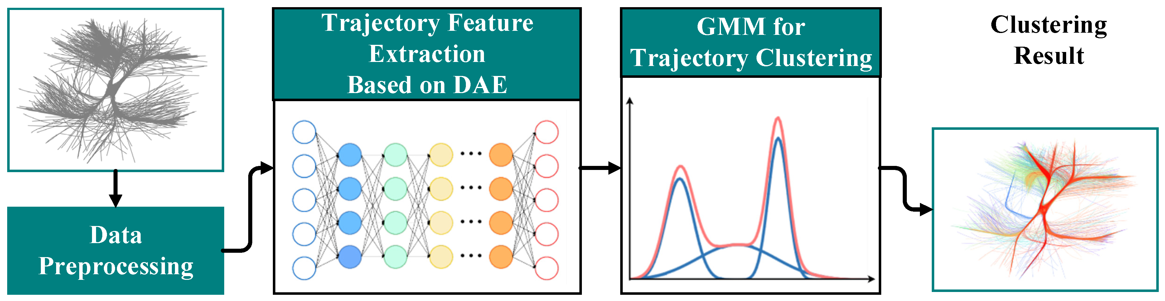
The general idea of this paper includes data preprocessing, trajectory feature extraction, and trajectory clustering, as shown in Figure 1. (1) Data preprocessing: Extract the trajectory data in the designated area of the airport terminal area and analyze the data quality. Then, transform the geographic coordinates into ENU coordinates and divide the trajectory into arrival and departure. (2) Trajectory feature extraction: The DAE model is used to map the trajectory data to a new set of features in another domain. The input data include time, longitude, latitude, altitude, speed, and heading. When the model is built, the parameters need to be adjusted continuously to reduce the error of input data reconstruction. The parameters mainly include the number of hidden layers and the number of hidden layer neurons. (3) Trajectory clustering: Use the GMM to cluster the new trajectory features and combine the commonly used indicators and visualization methods to evaluate the clustering effect.

2.1. Data Processing

In the airport terminal area, it is necessary to extract ADS-B data or radar data according to the specified horizontal and altitude range and use the value analysis method to analyze the null, duplicate, and abnormal values of the data preliminarily and deal with them. To simplify the calculation of space distance and present the changes of the aircraft trajectory more intuitively, it should convert the longitude and latitude data from the geographical coordinate system to the ECEF (Earth-Centered-Earth-Fixed) rectangular coordinate system, which takes earth mass center as the origin; the Z-axis points to the north pole, the X-axis intersects the Greenwich line and the equator on the sphere (longitude and latitude are both 0), and the Y-axis is determined according to the right-hand coordinate system. The coordinate conversion process is as follows:

Firstly, the flattening of ellipsoid f, eccentricity $e\_sq$, and radius of curvature $N$ corresponding to space spherical coordinate system are calculated:

$$f=\frac{a-b}{a}$$

(1)

$$e\_sq=f\times (2-f)$$

(2)

$$N=\frac{a}{\sqrt{1-e\_sq\times {(\sin \phi )}^2}}$$

(3)

where $\phi$ represents the radian corresponding to latitude, $a$ represents the radius of the earth’s major axis, and $b$ represents the radius of the earth’s minor axis. Then, the coordinate values X, Y, Z of the corresponding ECEF coordinate system are calculated:

$$X=(h+N)\times \cos \phi \times \cos \lambda$$

(4)

$$Y=(h+N)\times \cos \phi \times \sin \lambda$$

(5)

$$Z=[h+(1-e\_sq)\times N]\times \sin \phi$$

(6)

where $\lambda$ represents the radian corresponding to longitude, and $h$ represents the height.

However, the coordinate value in the ECEF rectangular coordinate system is very large. In order to express the relative position of the track points, the ECEF coordinates are further transformed into the ENU (East-North-Up) rectangular coordinate system with the center of the airport as the origin. The positive Z-axis coincides with the ellipsoid’s normal, the positive Y-axis points to the north, and the positive X-axis points to the east. Taking the ECEF coordinate of the center of the terminal area $(x_0,y_0,z_0)$ as the origin position, ${\phi }_0$ represents the radian corresponding to the latitude of the origin, ${\lambda }_0$ represents the radian corresponding to the longitude of the origin, and $h_0$ represents the height of the origin. The coordinate values xEast, yNorth, and zUp of the ENU rectangular coordinate system are calculated according to the origin coordinates:

$$xEast=-\sin {\lambda }_0\times (X-x_0)+\cos {\lambda }_0\times (Y-y_0)$$

(7)

$$yNorth=-\cos {\lambda }_0\times \sin {\phi }_0\times (X-x_0)-\sin {\lambda }_0\times \sin {\phi }_0\times (Y-y_0)+\cos {\phi }_0\times (Z-z_0)$$

(8)

$$zUp=\cos {\lambda }_0\times \cos {\phi }_0\times (X-x_0)+\cos {\phi }_0\times \sin {\lambda }_0\times (Y-y_0)+\sin {\phi }_0\times (Z-z_0)$$

(9)

Since arrival and departure flights have completely different operating modes, they need to be considered separately. Here, the extracted trajectory data can be directly divided into arrival and departure flights according to the origin and destination contained in the ADS-B data.

2.2. DAE for Trajectory Feature Learning

The feature learning algorithm aims to find a good representation of data for classification, reconstruction, visualization, and so on. At present, the most commonly used unsupervised methods in image feature extraction are PCA and autoencoder. The encoder and decoder of PCA are linear, while the autoencoder can be linear or nonlinear. PCA is only interested in the direction of maximum variance, but it does not fit well with many practical applications. By contrast, autoencoder has been successfully used in many image processing applications [35,36,37,38]. Therefore, this paper will use DAE to extract features from the original trajectory data.

In fact, DAE in this paper means Stack Autoencoder rather than traditional deep autoencoder. Stack Autoencoder and deep autoencoder only differ in the training process, and they have the same reconstruction function. However, due to the greedy layer-by-layer training of Stack Autoencoder, its coding ability is slightly worse. Nevertheless, the large number of aircraft trajectory points results in large data dimension, and the direct use of traditional deep autoencoder is not efficient. By contrast, Stack Autoencoder has relatively simple structure, high efficiency, and robustness.

An autoencoder is an artificial neural network that can learn the effective representation of input data without supervision. It is always composed of two parts: the encoder (or recognition network), which converts the input to the internal representation, and the decoder (or generation network), which converts the internal representation to the output. The dimensionality of the output of the encoder is usually lower than that of the input data so that the autoencoder can be effectively used for data dimensionality reduction. In addition, the autoencoder can also be used as a powerful feature detector for unsupervised deep neural network pre-training. The decoder can randomly generate new data that are very similar to the training data.

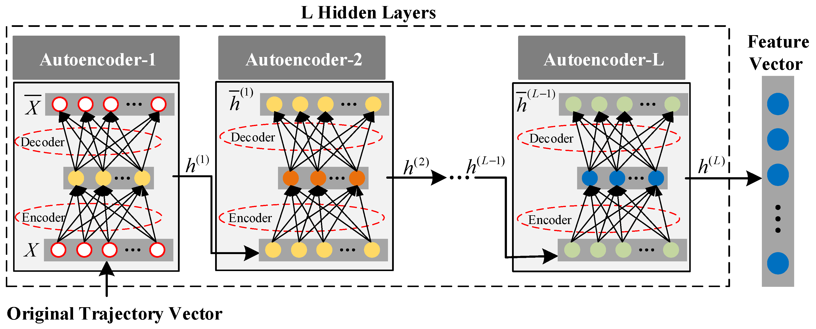
The autoencoder usually has the same architecture as the multi-layer perceptron (MLP), but the number of neurons in the output layer must be equal to the number of neurons in the input layer. As shown in the network structure of Figure 2, a simple autoencoder is a three-layer neural network structure that includes a data input layer, a hidden layer, and an output reconstruction layer. When a set of training datasets $X=\{X_1,X_2,\dots ,X_N\}$ are given, where $X\in R^{N\times n}$, $X_i\in R^n$, $n$ represents the number of neurons in the input layer; the encoder first encodes the input data and converts them into the hidden layer’s output $h_i^{(1)}$ based on Equation (10). The decoder decodes it to obtain ${\overline{X}}_i$ (that is, reconstructed $X_i$), as in Equation (11):

$$h_i^{(1)}=f(X_i)={\sigma }_f(W_f{X}_i+b_f)$$

(10)

$${\overline{X}}_i=g(h_i^{(1)})={\sigma }_g(W_g{h}_i^{(1)}+b_g)$$

(11)

where $W_f\in R^{n\times n_1}$ is the encoder weight matrix, $n_1$ is the number of neurons in the hidden layer, $b_f\in R^{n_1}$ is the encoder bias vector, and ${\sigma }_f$ is the encoder activation function; $W_g\in R^{n_1\times n}$ is the decoder weight matrix, $b_g\in R^n$ is the decoder bias vector, and ${\sigma }_g$ is the decoder activation function. Non-linear functions are usually used as activation functions in networks, such as sigmoid function, hyperbolic tangent function, and rectified linear unit function, and sigmoid function is used here. Since the autoencoder tries to reconstruct the input, the output is usually called reconstruction, and the loss function is the reconstruction loss. When the reconstruction is different from the input, the reconstruction loss will penalize the model. The model can choose different loss functions according to different criteria, such as $L_i$ norm and entropy. Here, we choose $L_2$ norm. Let us take the first autoencoder in Figure 2 as an example that is trained by minimizing the reconstruction error $L(X_i,{\overline{X}}_i)$ to obtain the model’s best parameters, denoted as ${\theta }_1$, as shown in Equation (12).

$$\theta =\underset{{\theta }_1}{\arg \min }L\left(X_i,{\overline{X}}_i\right)=\underset{{\theta }_1}{\arg \min }\frac{1}{2}{\displaystyle \sum _{i=1}^n{\Vert x_i-{\overline{x}}_i\Vert }^2}$$

(12)

DAE is a deep neural network composed of multiple autoencoders, and the input of the next encoder comes from the output of the previous encoder. This structure helps DAE to learn more complex features. As shown in Figure 2, given the DAE of L hidden layers, the training set is used as input, the first hidden layer is trained as the encoder and used as the input layer of the second hidden layer, and so on. The $k$th hidden layer is used as the input layer of the $k+1$th, so that multiple autoencoders can be stacked in layers [39]. Figure 2 explains the training process of the model. It trains a shallow autoencoder and then stacks all autoencoders into DAE instead of training the whole DAE. The final reconstruction error combines the loss of all hidden layers. The training process is shown in Algorithm 1:

Algorithm 1 Feature extraction of trajectory data based on DAE

Input:  Standardized trajectory data.  The number of hidden layers $L$ and units $n_i,i=1,\dots L$. Output:  Extracted feature data.  Optimal model parameters $\theta =\{{\theta }_1,{\theta }_2,\cdots ,{\theta }_L\}$. Algorithm—DAE pre-training:  1. Initialize the weight matrix $W$ and the bias vector $b$ randomly.  2. Train hidden layers through greedy layer-wise training.  3. The $k$th layer is regarded as the input layer of the $k+1$th, and for the first layer, the standardized trajectory data are used as the input.  4. In the $k$th layer, the encoder’s parameters are determined by minimizing the objective function such as Equation (12), and Adam optimizer is used to train the model.  5. Output extracted features, optimal parameter set $\theta$.

2.3. Trajectory Clustering with GMM

At present, the clustering algorithms widely used in air traffic pattern recognition include K-Means [4], K-medoids [12], DBSCAN [18], and their improved algorithms. Compared with them, GMM can provide the probability that the sample belongs to each Gaussian component and can be further used for trajectory probability generation and trajectory anomaly detection. Given the advantages of GMM, this paper will use GMM for clustering analysis. GMM learns the probability density function of all samples and calculates the probability assigned to each cluster. Assuming that all samples obey the Gaussian distribution, the model is composed of K Gaussian distribution weights [40]:

$$\begin{array}{ll}p(x)& ={\displaystyle \sum _{k=1}^{K}p(k)p(x|k)}\hfill \\ & ={\displaystyle \sum _{k=1}^K{\pi }_{k}N(x|{\mu }_k,{\sum }_k)}\hfill \end{array}$$

(13)

where ${\pi }_k$ is the weight of the $k$th Gaussian distribution, $N(x|{\mu }_k,{\sum }_k)$ is the probability density function of the $k$th Gaussian distribution, the mean is ${\mu }_k$ and the variance is ${\sum }_k$. The model needs to estimate the parameters of ${\pi }_k$, ${\mu }_k$, and ${\sum }_k$ to estimate the probability density function, which can use the maximum likelihood method to maximize the probability value of the sample point on the estimated probability density function. However, the probability is generally very small. When the sample size is large, the result of their multiplication is very small, which is easy to cause floating-point underflow. Therefore, we usually take the log of it to turn the product into a sum and obtain the log-likelihood function:

$$\begin{array}{cc}\log (p(x))& ={\displaystyle \sum _{i=1}^N\log (p(x_i))}\hfill \\ & ={\displaystyle \sum _{i=1}^N\log ({\displaystyle \sum _{k=1}^K{\pi }_{k}N(x_i|{\mu }_k,{\sum }_k)})}\hfill \end{array}$$

(14)

where $N$ is the number of samples. The variable to be sought is generally differentiated to maximize the log-likelihood function for parameter estimation. However, there is a summation in the logarithmic function in Equation (14), and the derivative will be very complicated, so the EM algorithm is used to solve the problem instead of the derivative. The basic idea of the EM algorithm is to calculate the posterior probability of the hidden variable as its current estimated value according to the initial value of the model parameters or the result of the previous iteration, and then maximize the likelihood function to obtain the new parameter value. The algorithm includes E step and M step, as shown in Algorithm 2. The specific steps are as follows:

(a) E step: Estimate the probability that each component generates the sample. The probability that sample $x_i$ is generated by the $k$th component is:

$$\gamma (i,k)=\frac{{\pi }_{k}N(x_i|{\mu }_k,{\sum }_k)}{{\displaystyle {\sum }_{j=1}^K{\pi }_{j}N(x_i|{\mu }_j,{\sum }_j)}}$$

(15)

since ${\mu }_k$ and ${\sum }_k$ in Equation (15) are the parameters to be estimated, it is necessary to assume that ${\mu }_k$ and ${\sum }_k$ are known when calculating $\gamma (i,k)$ for the first time, and then continue to calculate new values through iteration. The K centroid coordinates obtained by K-Means clustering are used as the initial mean of K Gaussian components of GMM, and the weight and variance are calculated.

(b) M step: Estimate the parameters of each component. Assuming that $\gamma (i,k)$ obtained in E step is the correct probability of sample $x_i$ generated by the $k$th component, it can also be regarded as the contribution of the $k$th component to the generation of sample $x_i$, that is, $\gamma (i,k)x_i$ of sample $x_i$ is generated by the $k$th components. When all samples are considered, it can actually be seen that the $k$th component generating $\gamma (1,k)x_1,\dots , \gamma (N,k)x_N$. Since each component is a standard Gaussian distribution, the parameters in the maximum likelihood function can be obtained:

$${\mu }_k=\frac{1}{N_k}{\displaystyle \sum _{i=1}^N\gamma (i,k)x_i}$$

(16)

$${\sum }_k=\frac{1}{N_k}{\displaystyle \sum _{i=1}^N\gamma (i,k)(x_i-{\mu }_k){(x_i-{\mu }_k)}^T}$$

(17)

where $N_k={\displaystyle {\sum }_{i=1}^N\gamma (i,k)}$, and ${\pi }_k$ is estimated to be $N_k/N$. At this time, the log-likelihood function value of Equation (14) can be calculated.

(c) Repeat the first two steps until the log-likelihood function value converges.

Algorithm 2 Trajectory feature clustering analysis algorithm based on GMM

Input:  Features extracted based on DAE.  Number of Gaussian components K. Output:  Suitable GMM model parameter set $\varphi =\{{\pi }_k,{\mu }_k,{\sum }_k\},k=1,\dots ,K$. Algorithm:  1. Initialize GMM parameters $\varphi$ using K-Means result.  2. E step: Use Equation (15) to estimate the prior probability of input data generated by each Gaussian component.  3. M step: Use Equations (16) and (17) to update each component’s parameters.  4. Use Equation (14) to calculate the log-likelihood function value: If $\log (p(X|{\varphi }_t))-\log (p(X|{\varphi }_{t-1}))<\epsilon$, $\epsilon$ is the termination threshold; that is, if the likelihood function converges, the iteration is stopped, or else $\varphi ={\varphi }_t$, go back to step 2.  5. Output parameter set $\varphi$.

3. Experimental Results and Discussion

This paper takes the terminal airspace of Guangzhou Baiyun International Airport in China as a case to verify the proposed clustering method. The experiment uses the Python programming language, and the computer is configured with Windows 10 system, 8-core i5 CPU, and 64 GB RAM.

3.1. Data Preparation

The experiment uses six months of ADS-B trajectory data collected from September 2018 to February 2019 for data preprocessing. The data cover all flights taking off and landing from Guangzhou Baiyun International Airport and are composed of aircraft position (measured by WGS84 latitude/longitude), pressure altitude (m), speed, heading, recording time, aircraft type, and flight information.

First of all, it is found that duplicate records and records with missing values and outliers in attributes account for a very small proportion through the preliminary quality analysis of the dataset, so delete them directly. Next, the trajectory data are extracted with the airport as the center, a radius of 50 km, and a height of 4 km, and their geographic coordinates are converted into ENU coordinates. Then, they are divided into arrival and departure according to requirements. All departure (arrival) trajectory sequences use the runway’s midpoint as the starting point (endpoint) of the trajectory. Because the significant difference between the arrival trajectory and the runway midpoint is farther than departure, the length of the arrival trajectory sequence chosen is longer than that of departure. Finally, 10,554 arrival trajectories with a length of 385 and 17,438 departure trajectories with a length of 248 were obtained. The results are shown in Figure 3.

The min-max normalization is used to standardize the trajectory data and map them to [0, 1] to eliminate the influence of different dimensions, which is convenient for feature extraction by DAE.

3.2. Evaluation Index

To evaluate the clustering effect, the sum of the squared error (SSE) within the cluster, silhouette coefficient (SC), CH index, and DB index are used as evaluation indexes, and they are defined as follows [41]:

$$SSE={\displaystyle \sum _{j=1}^K{\displaystyle \sum _{p\in C_j}dist{(p,{\mu }_j)}^2}}$$

(18)

$$SC=\frac{1}{N}{\displaystyle \sum _{i=1}^N\frac{b_i-a_i}{\max \{a_i,b_i\}}}$$

(19)

$$CH=\frac{{\displaystyle \sum _{j=1}^{K}dist{({\mu }_j,\mu )}^2}/(K-1)}{SSE/(N-K)}$$

(20)

$$DB=\frac{1}{K}{\displaystyle \sum _{i=1}^K\max \{\frac{D_i+D_j}{dist({\mu }_i,{\mu }_j)}\}}$$

(21)

In Equation (18), $C_j$ represents the $j$th cluster, $p$ is the sample in $C_j$, and ${\mu }_j$ is the mean of all samples in $C_j$. SSE measures the compactness within a cluster by calculating the sum of the squares of the distances between the samples in the cluster and the center of the cluster, and the smaller the SSE, the better. In Equation (19), $a_i$ is the average distance between the sample $p_i$ and other sample points in the same cluster, $b_i$ is the average distance between the sample $p_i$ and all the sample points in the nearest cluster, $b_i-a_i/\max \{a_i,b_i\}$ is the silhouette coefficient of the sample $p_i$, and $N$ is the total number of samples. SC is the average silhouette coefficient of all sample points, which is called the silhouette coefficient of clustering results: the larger the better. In Equation (20), $\mu$ is the mean of all samples, and ${\displaystyle {\sum }_{j=1}^{K}dist{({\mu }_j,\mu )}^2}$ measures the separation degree by calculating the sum of the squares of the distances between the center points of various clusters and the center points of all samples. The CH index is obtained by the ratio of separation and compactness, indicating that the larger the value, the closer the cluster itself, and the more scattered they are between clusters. In Equation (21), $D_i$ is the average distance between the sample in the cluster $C_j$ and the center of the cluster. The smaller the DB, the smaller the distance within the cluster, and the larger the distance between the clusters.

3.3. Performance Analysis

The DAE model includes two modules: encoder and decoder; so, the model parameters to be determined mainly include the number of hidden layers of the encoder and decoder and the number of neurons in each hidden layer. Too few hidden layers or neurons may lead to poor network learning ability, and it cannot effectively represent high-dimensional data; while too many will increase the training time and affect the operation efficiency, so appropriate parameters must be selected. For arrival trajectories, the range of encoding (decoding) hidden layers is {3, 4, 5, 6, 7}, and the setting range of hidden layer nodes is {1024, 512, 256, 128, 64, 32, 16}. For departure trajectories, the range of layers is {2, 3, 4, 5, 6}, and the range of hidden layer nodes is {512, 256, 128, 64, 32, 16}. The best DAE model parameters are obtained by implementing different parameter combinations, as shown in

Table 1. Parameter settings for the model.

Trajectory Type	Number of Hidden Layers	Number of Nodes
Departure trajectory	1	512
	2	256
	3	128
	4	64
	5	39
Arrival trajectory	1	1024
	2	512
	3	256
	4	128
	5	64
	6	28

.

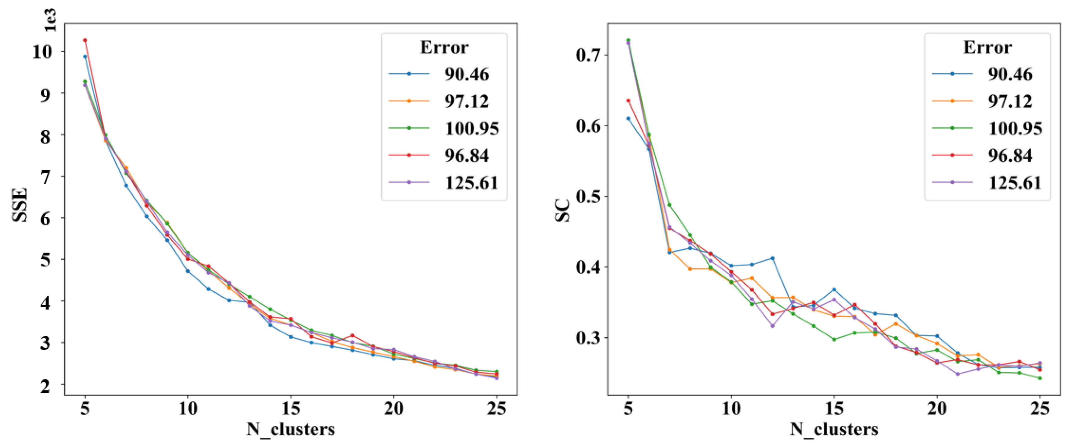
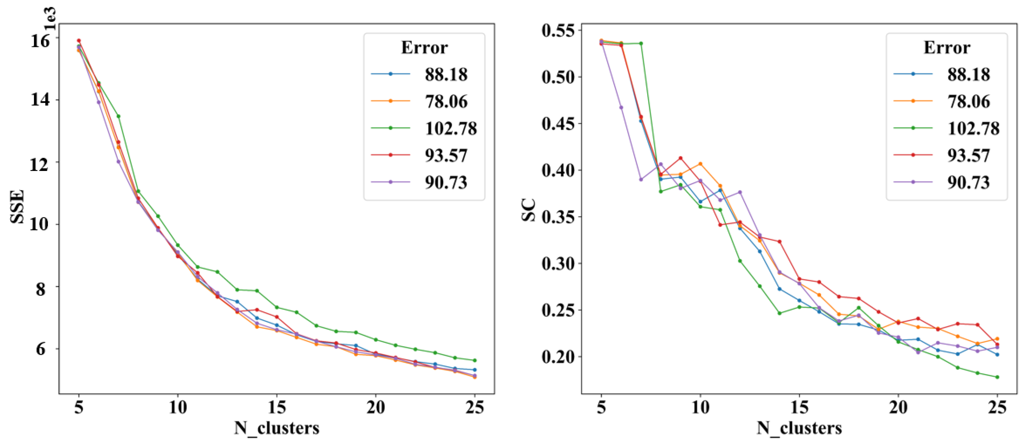
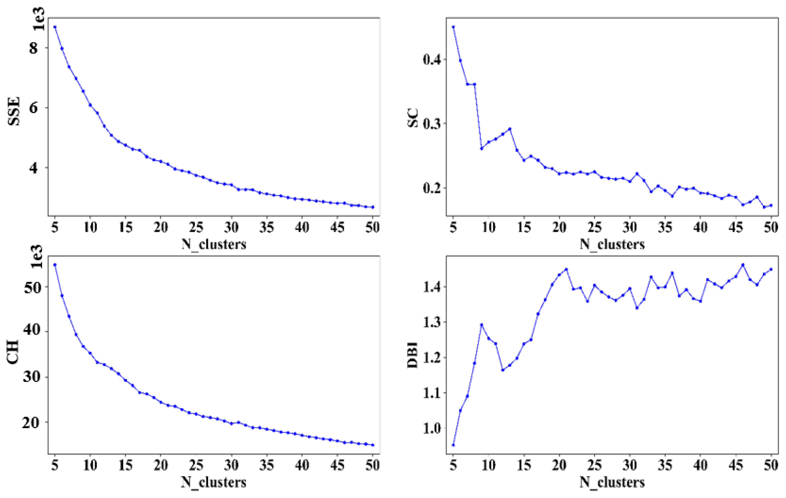
Features are extracted under different parameters. The clustering results are compared to observe whether the feature extraction effect will affect the later clustering effect. The root mean square error (RMSE) is used to calculate the error between the reconstruction result of the DAE decoder and the original data to measure the effect of DAE feature extraction. As shown in Figure 4 and Figure 5, GMM is used to cluster the output features of DAE models with different reconstruction errors. It is found that regardless of the arrival or departure trajectory, with the increase in reconstruction errors, the SSE will increase, the SC will decrease under different cluster numbers, and the overall clustering effect will be worse. Therefore, it is necessary to reduce the DAE model feature reconstruction error as much as possible to improve the effect of later trajectory clustering.

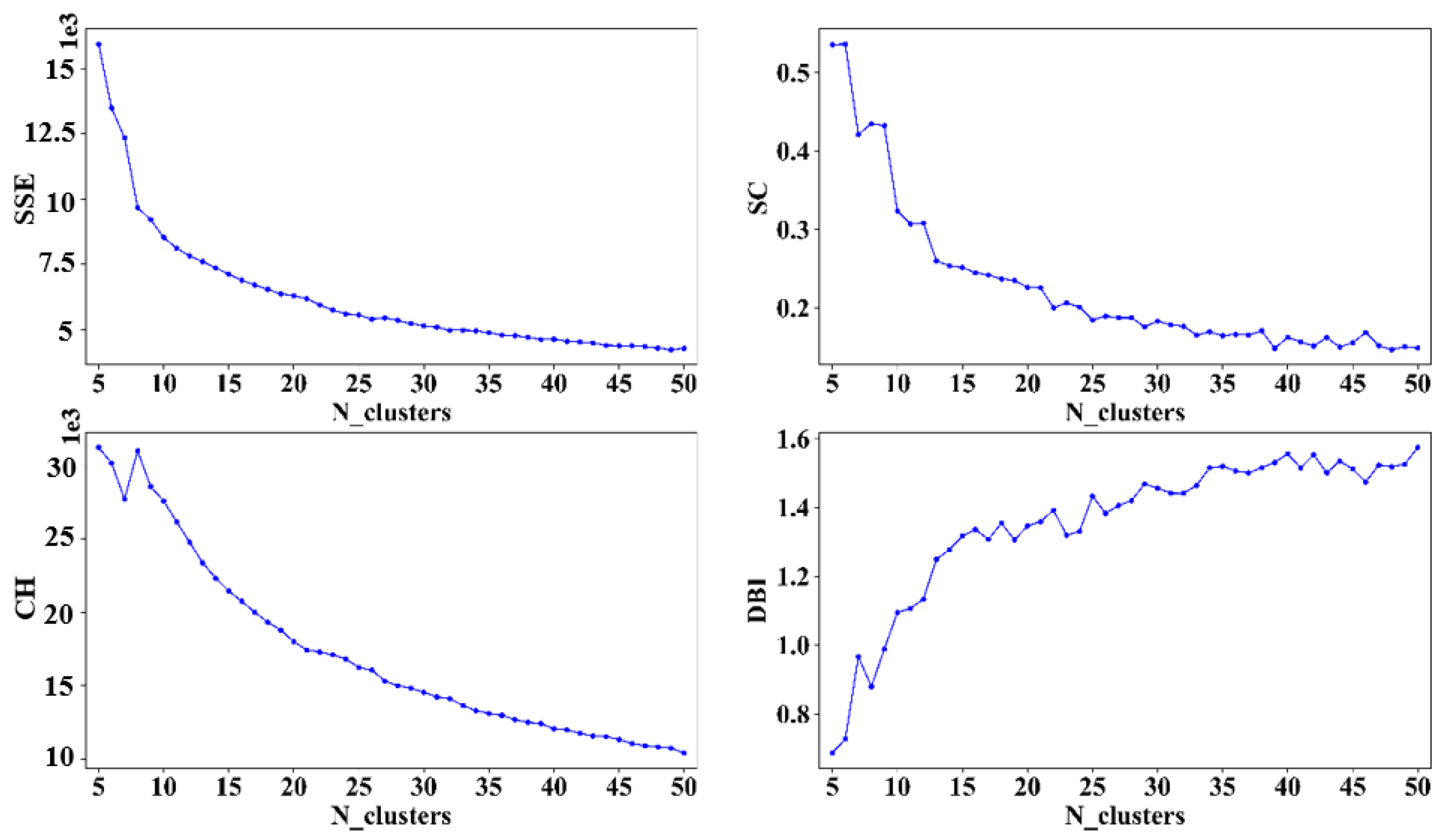
After using the best DAE model to extract the features of all trajectories, GMM is used to cluster the extracted features. As shown in Figure 6 and Figure 7, the elbow method is used to select the appropriate number of clusters K. Since the features extracted by DAE are clustered here, and the goal is to observe different patterns of trajectories, it is ultimately necessary to combine the category labels and the original trajectory data to calculate various index values to select the parameters with the best clustering effect. In addition, clustering is an unsupervised learning algorithm, and there is usually no strict reference standard to select parameters. Therefore, in addition to the four clustering evaluation indexes, we also determine the parameters of the clustering model combined with the actual situation. It can be seen from the figure that for arrival trajectories, when K < 30, the SSE decline amplitude is larger, and when K > 30, the SSE decline amplitude slows down and tends to be gentle; when K = 30, SC is larger than adjacent SC; the downward trend of CH and SSE is similar; when K > 30, the downward trend begins to slow down; when K = 30, DB index is also smaller than adjacent values, therefore, the cluster number of 30 is more appropriate. Similarly, the optimal number of clustering is selected as 40 for the departure trajectories.

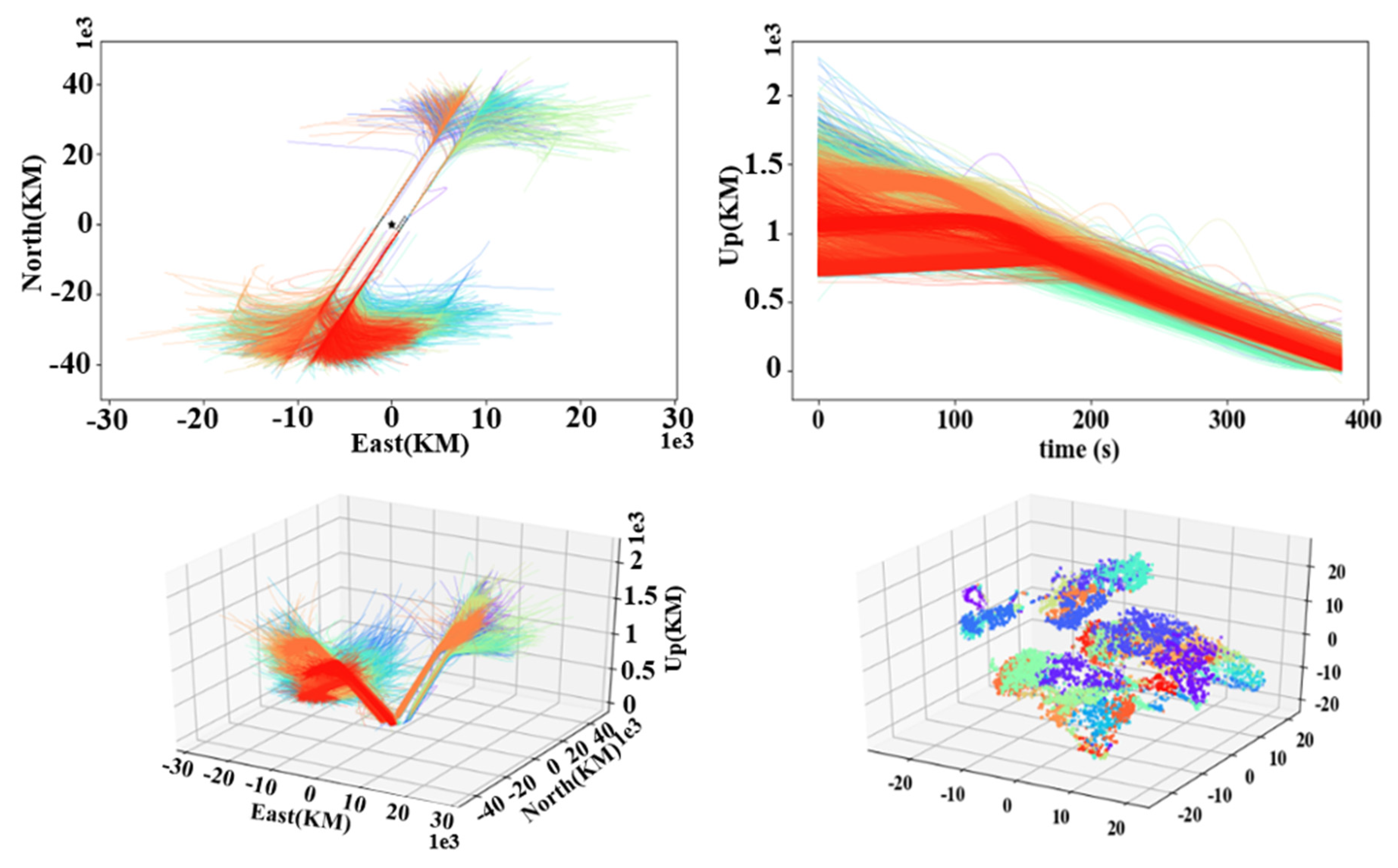
According to the selected optimal cluster number K, the arrival and departure trajectories are clustered. As shown in Figure 8, the first three subgraphs, respectively, show the horizontal, vertical, and 3D visualization results of each cluster of the arrival trajectories. Among them, the trajectories with similar altitude changes but different heading directions are basically classified significantly, indicating that the extracted features include the features of trajectory turning points. At the same time, the trajectories with similar heading and different altitudes are also significantly separated, which shows that the clustering process considers the horizontal position and the changes in altitude. In summary, it can be considered that clustering the extracted arrival trajectory features can indeed effectively classify different patterns. To visualize the classification results of high-dimensional trajectories more intuitively, the t-SNE method is used to reduce the dimensionality of each trajectory to a 3D space for observation. As shown in the last subgraph, it can be found that the trajectory set has good separability and is not disorderly, proving that clustering results are meaningful.

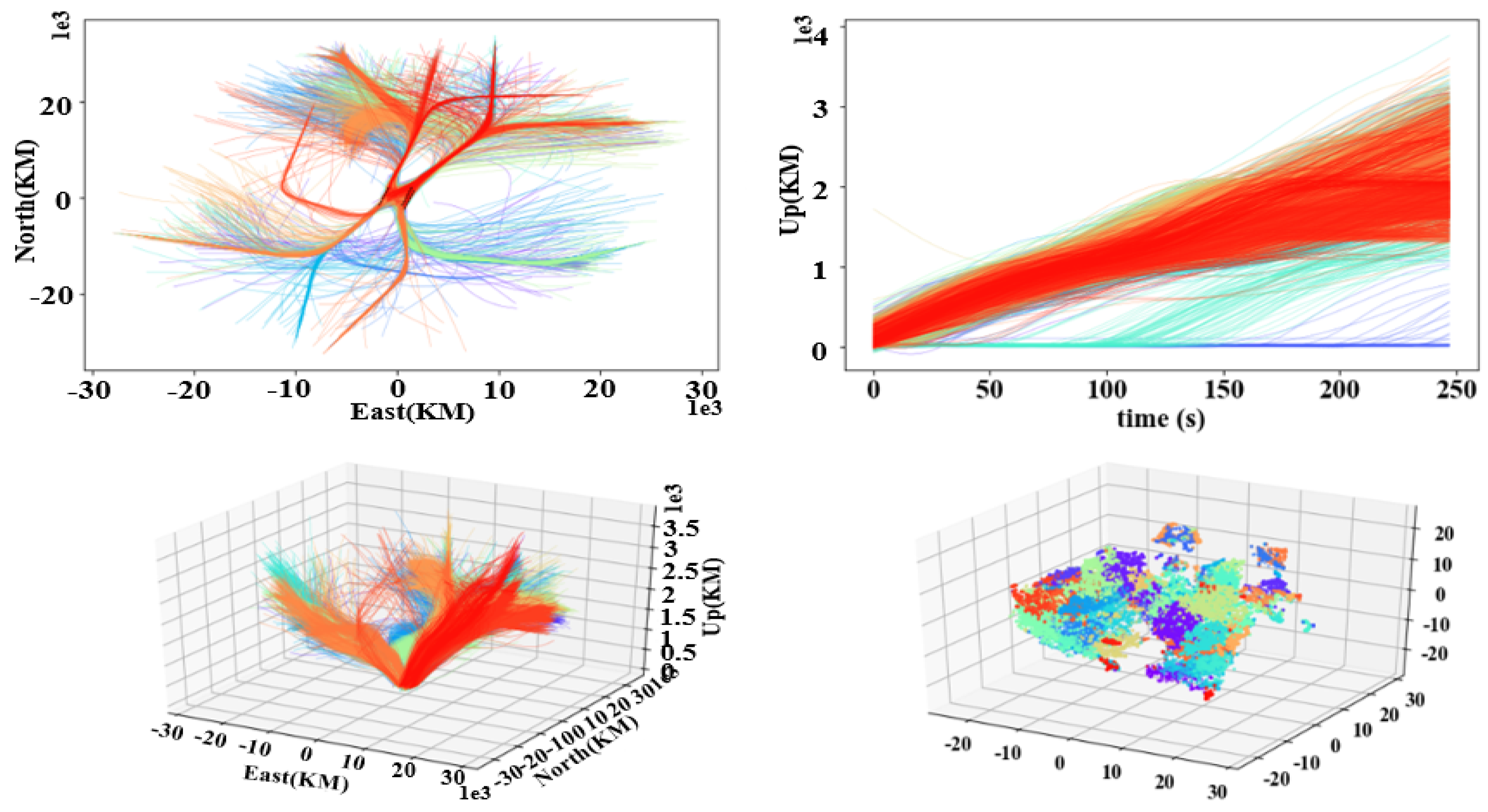
The first three subgraphs in Figure 9 show the horizontal, vertical, and 3D visualization results of each cluster of the departure trajectories. Similar to the arrival trajectories, trajectories with similar altitude changes but different departure directions and trajectories with similar departure directions and different altitudes are successfully separated. The last subgraph is the visualization result of reducing the dimensionality of each trajectory to a 3D space using the t-SNE. It can also be found that the departure trajectory set has good separability. Therefore, the departure trajectories are similar to the arrival trajectories and have an excellent clustering effect.

The experiment mainly observes whether the feature extracted from the DAE model has a good effect in terms of performance and speed. If the clustering results are better and the running speed is faster, the clustering framework proposed in this paper is meaningful.

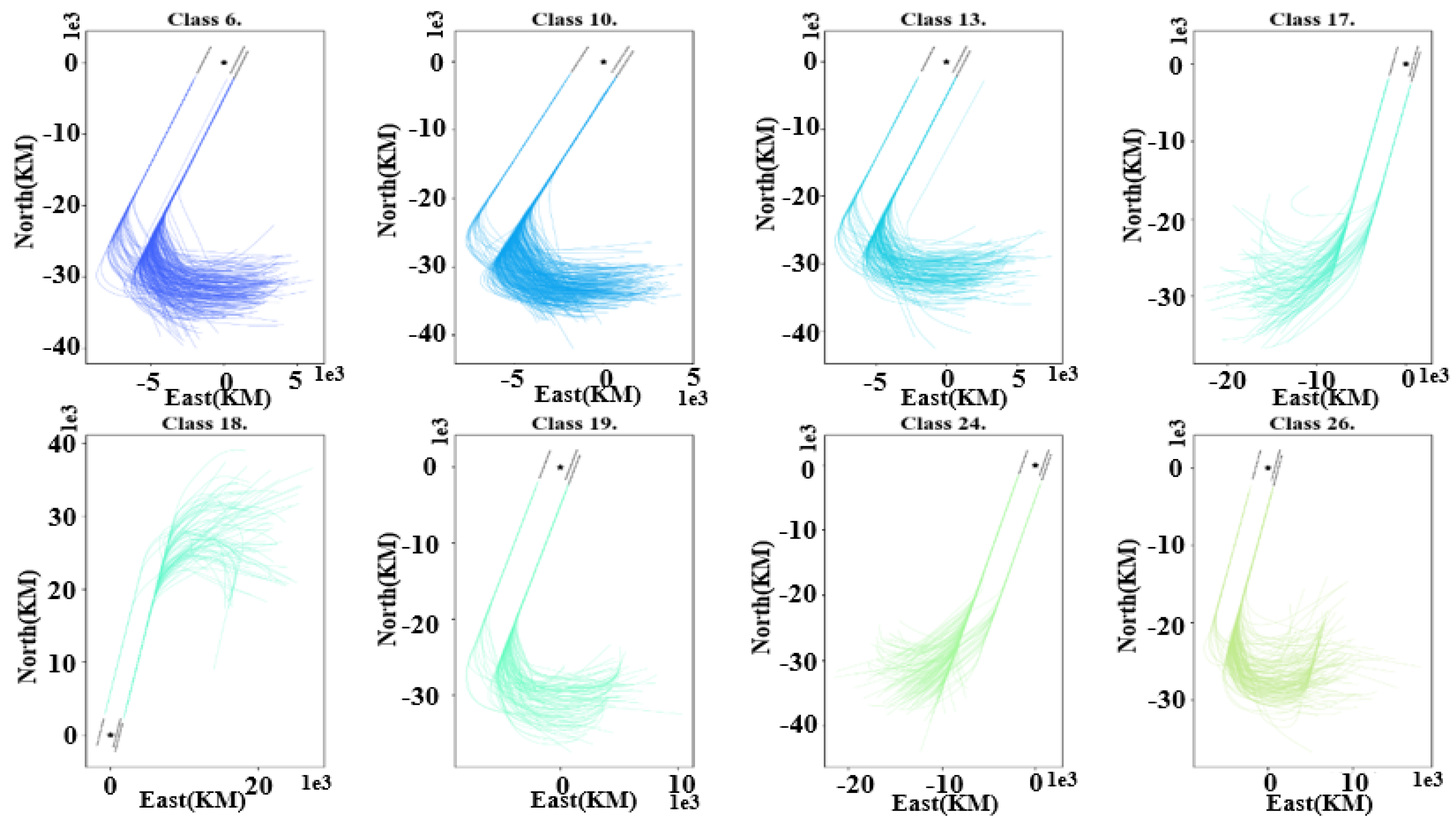
Firstly, in terms of performance, it visually displays the clustering results. As shown in Figure 10, the visualization results of clustering the extracted arrival trajectory features are shown. For clear display, each category is displayed separately. Due to a large number of clusters, only some of the clusters are displayed randomly. It can be seen from the figure that the trajectories in each category basically follow the same approach procedure and have the same heading and turning angle. Except for a few trajectories, most trajectories have no apparent deviation. Although categories 6, 10, 13, 17, and 24 have almost the same arrival heading and trajectory trend, they are divided into different categories due to the difference in descent levels. Therefore, the effect of clustering of the extracted features is better. It also shows that the extracted features can indeed reflect the location, height, and heading of the trajectory.

Figure 11 shows the visualization results for each cluster of departure trajectories. It can be seen from the figure that the trajectories in each category basically have the same departure pattern, among which categories 5, 10, 26, and 32, and categories 12 and 30 have almost the same departure heading and trajectory trend. Still, they are divided into different categories due to the differences in climbing levels. Although the trajectories of each cluster are relatively concentrated, a few trajectories have some deviations, which may be shown in Figure 3 that the departure trajectories are usually more dispersed than the arrival trajectories, and the arrival trajectories will not have large deviations because the airport terminal arrival routes are generally fixed. In general, the clustering visualization results using the features extracted from the DAE model are better, showing that this paper’s clustering framework is feasible in performance.

Since dimensionality reduction of high-dimensional data can significantly reduce the amount of data and storage space and effectively compress the original data, it will definitely improve clustering efficiency [42].

Table 2. Comparison of the clustering time of arrival trajectories in the two cases.

Sample Size	DAE + GMM(S)	GMM(S)
100	0.12	0.16
500	0.14	0.45
1000	0.20	0.70
5000	0.58	6.03
10,000	1.09	13.03

and

Table 3. Comparison of the clustering time of departure trajectories in the two cases.

Sample Size	DAE + GMM(S)	GMM (S)
100	0.16	0.16
500	0.22	0.30
1000	0.28	0.53
5000	0.94	4.62
10,000	1.67	9.72

, respectively, list the time consumption of different sample sizes in clustering the original data and the extracted features. It can be found that with the gradual increase in the sample size, clustering the reduced-dimensional data can quickly shorten the clustering time and speed up the clustering. Once the amount of data reaches 10 million or even larger, the clustering method proposed here can play a huge advantage. Simultaneously, the speed improvement of departure trajectories is not as fast as that of arrival because its operation patterns are more complex than that of arrival.

4. Conclusions

This paper proposes an aircraft trajectory clustering method, including data processing, feature extraction, and clustering. First, the trajectory data within the designated terminal area are extracted from the massive and complex raw data and processed into a form suitable for dimensionality reduction. Then, the DAE model is used to reduce their dimensionality and extract features that can better reflect the trajectory information. Finally, the GMM is used to cluster the new features extracted. To prove the feasibility of the proposed clustering method, the four indicators of SSE, SC, CH, and DB were used to evaluate the clustering results, and the visualization of various trajectories confirmed the rationality of the clustering results, which showed the effectiveness of the method proposed in this paper. At the same time, this method can quickly shorten the clustering time and improve the clustering efficiency, which has certain advantages.

The method proposed in this paper is based on a data-driven suitable-for-terminal-area trajectory and can be applied to trajectory pattern mining in the cruise phase. In future research, we can extract the typical central trajectory according to the output of the clustering analysis, and compare it with the actual operation of the arrival and departure flight procedures and airspace division, thereby optimizing the airspace structure. Besides, we will consider extending this method to assist in trajectory prediction [43,44], hoping to extract various operating patterns of trajectories through cluster analysis and establish prediction models, thereby improving trajectory prediction accuracy. Similarly, we can also perform abnormal trajectory detection for each cluster to improve detection accuracy. Ultimately, we hope that the clustering method can guide the real-time decision support system.