1. Introduction
The first object of interstellar origin discovered in the Solar System was the ’Oumuamua on October 2017 [
1,
2], detected by the Pan-STARRS1 telescope system at the Haleakala Observatory, Hawaii. Its name, in the local language, could be translated as
the first messenger arriving from far away. Two years later, on August 2019, the amateur astronomer Gennady Borisov spotted a second extrasolar visitor from the Crimean Peninsula, the interstellar comet Borisov [
3]. Although only two reported sightings of such interstellar objects (ISO) (Eubanks et al. [
4] or Rice and Laughlin [
5]) have been documented, these findings have been a complete revolution and have contributed to the opening of new research areas. Despite their unknown provenance, they provide exceptional insights into the behavior and composition of bodies in other planetary systems.
The population of such bodies has also been a subject of study in recent years. The discovery of two of them in such a short interval of time suggests that more of these objects could have been ejected from their respective planetary systems and could be wandering through space. The Large Synoptic Survey Telescope (LSST) at the Vera C Rubin Observatory in Cerro Pachón, Chile, is expected to progressively increase the detection rate of such bodies, with similar characteristics to those of ’Oumuamua [
5]. Future detections could provide useful statistics for a better understanding of their originary planetary systems, as well as the ejection process they undergo and their nature [
6]. On the other hand, the probability of future near-Earth trajectories of such objects also opens the door to the design of interception missions to study them or mitigate the collision risk, if necessary.
Different types of observations can provide information about these interstellar visitors [
7,
8,
9], promoting the need to investigate them more closely. Although the objectives of interception missions may vary from case to case, Moore et al. [
10] proposed the following three science goals, which could be accepted as common to any of these missions:
- (1)
Determine whether the interstellar object was formed in an environment or system with a similar chemical composition to that of the Solar System;
- (2)
Determine whether it resembles in shape and physical behavior any of the known classes of objects that populate the Solar System;
- (3)
Determine whether it contains any prebiotic traces necessary for the existence of life.
With these premises, Moore et al. have developed a mission concept for intercepting an interstellar object, with an emphasis on the scientific equipment that should be on board. While the first two objectives listed above can be partially fulfilled by observations in the vicinity of the ISO’s surface, the extraction of material from inside the body would allow a more precise reconstruction of its origins, as well as being strictly necessary for the detection of prebiotic material. They therefore propose the inclusion of a collision phase using an impactor in the mission, capable of excavating material from the innermost layers of the object, something that has already been done for the Solar System’s comet Tempel1 with the Deep Impact mission [
11] and for the comet 67P/Churyumov-Gerasimenko with the spacecraft Rosetta and Philae [
12]. Other celestial bodies such as C/2016 U1 (NEOWISE) [
13] are also objects of possible studies.
The mission strategies currently being investigated follow two distinct lines of study. There are those aimed at pursuing and finally capturing (with or without collision) one of the interstellar objects already sighted. These missions are of very long duration and high energy cost, since both bodies are at a great distance from the Earth. This is the framework of the Lyra Project, presented by Hein et al. [
14] as part of the Initiative for Interstellar Studies (I4IS), which aims to determine the feasibility of a future interception of ’Oumuamua. The same team is also working on a similar mission project for the interception of Borisov [
15].
On the other hand, ESA, in partnership with JAXA, has been working since 2019 in missions to intercept future interstellar objects, for example, the Comet Interceptor mission planned for 2029 [
16]. In the first step, it will head for the vicinity of the L2 Lagrange Point of the Earth–Sun system. Thus, it will remain at that point until a long-period comet or an ISO is detected, whereupon an impulse will be applied in order to change the probe’s orbit and direct it towards the interception. The rendezvous would take place at an interval close to its perihelion, requiring less energy capacity and significantly reducing the mission duration. The ESA strategy is therefore to wait for further sightings and to prepare the necessary structure so that the initiation of the trajectory takes place at the shortest interval after detection. Moore et al. [
10] propose to design missions strictly intended for the study of ISOs, since they could not have a cometary nature. These missions could follow a similar launch strategy as the Comet Interceptor.
The Lyra project is not the only one studying the feasibility of intercepting the first interstellar visitors to the Solar System. Seligman and Laughlin [
17] have investigated the interception of extrasolar bodies that may appear in the future by means of a rapid response, taking as an example the orbit of ’Oumuamua and assuming that it would have been detected early enough to reach it before it escaped from the Solar System. Both studies use Lambert’s problem formulation for the determination of the optimal interception trajectories. However, they do not introduce the orbital perturbations inherent to the interplanetary journey of the vehicle. In [
18], the authors modify Lambert-type trajectories for low Earth orbits considering the perturbations due to Earth’s oblateness and atmospheric drag. In this sense, our work adopts a similar approach with different methodology, taking into account the effects of the most significative perturbations accelerations on the target body and on the vehicle, such as solar radiation pressure (SRP) and gravitational perturbations of the inner and large-mass planets. Moreover, following a similar strategy as the Comet Interceptor [
16], Lagrange points are considered as starting points for the interception maneuver of the extrasolar object. The consideration of the aforementioned perturbations allows for correcting the impulsive maneuver (both in magnitude and direction) by means of an algorithm, ensuring a highly accurate trajectory design. The study has been applied to the possible interception of the first detected extrasolar object (’Oumuamua) and can be used to estimate the maneuvers of future interceptions of other bodies.
This paper is organized as follows.
Section 2 describes the methodology followed for solving the interception problem, emphasizing on the perturbation model selected. The algorithm implemented for the calculation of the optimal trajectory and the iterative scheme developed for calculating the necessary corrections for the effect of the perturbations are also shown.
Section 3 presents the application of the developed model for interception the ’Oumuamua, assuming its early detection. The results are shown in the form of porkchops, orbital trajectory plots and tables with the optimal impulses. Finally,
Section 4 summarizes the main conclusions drawn from the study carried out.
2. Methodology
This section presents the main characteristics of the mission for which the tool described in this paper is designed.
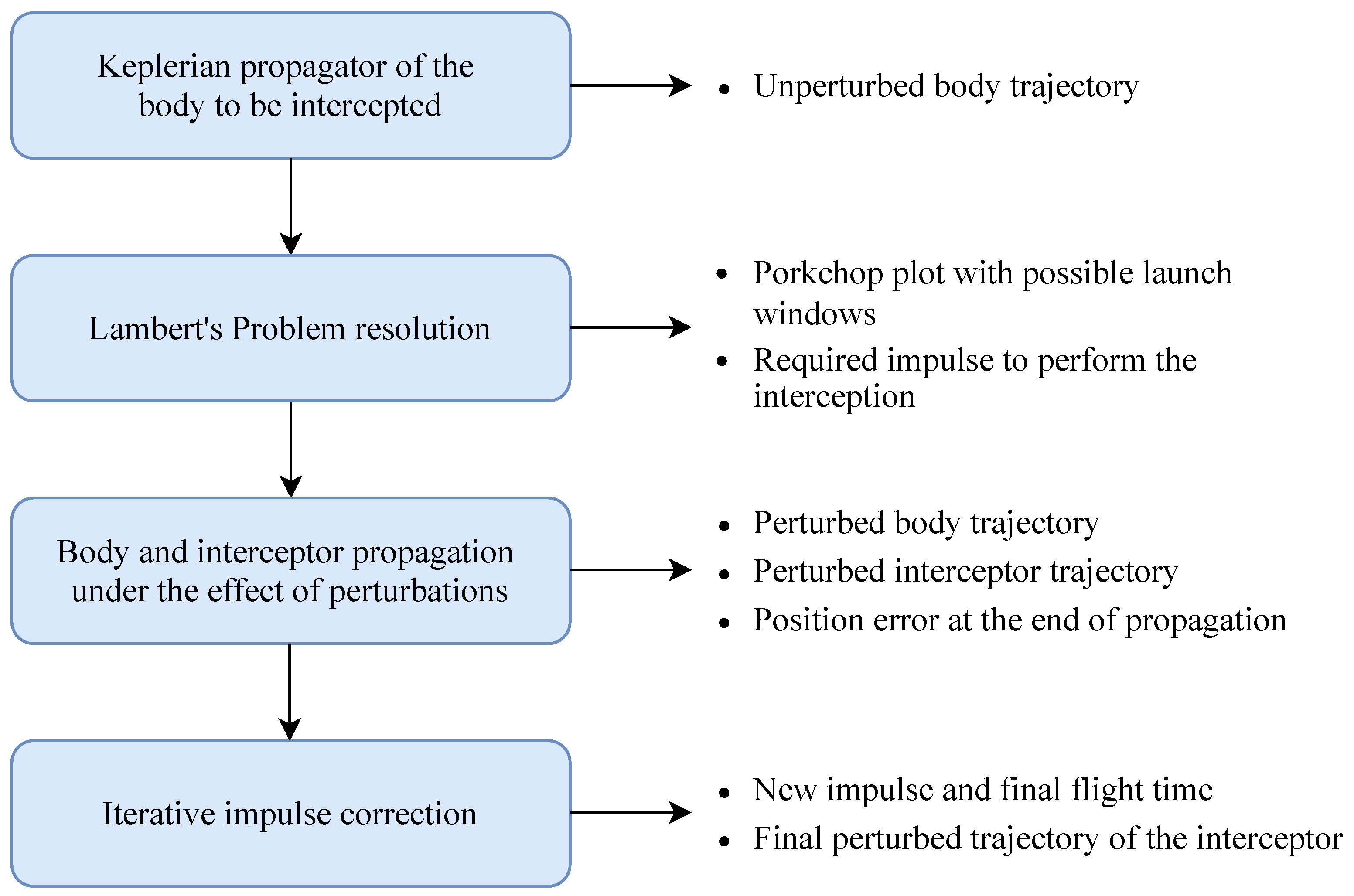
Figure 1 schematically depicts the approach followed to determine the optimal interception trajectory. First, Keplerian propagation is performed to determine the unperturbed orbit of the detected extrasolar body. An ephemeris of the body is then created to assess whether it represents a real risk to Earth and to make the first assessments of the feasibility of carrying out an interception mission. In a second phase, the Lambert’s problem is solved, and a mapping or porkchop plot of the launch windows and their energy cost is represented. By analyzing these results, the optimal interception trajectory and the necessary impulse to carry it out are determined. Since the Lambert’s problem addresses only ideal trajectories, without considering perturbations, it is necessary to include a third step in the process. In this third phase, both the extrasolar body and the interceptor are propagated under perturbed conditions. This provides more realistic trajectories that allows calculating, through an iterative process, the necessary modifications on the initial impulse to guarantee the interception. These modifications are performed in both magnitude and direction.
2.1. Description of the Mission
The designed tool aims to determine the optimal trajectory to intercept an object of extrasolar origin given its position and velocity vectors at a given epoch. If there is a risk of collision, the mission design will be different (see, for example, [
19]), adapting the restrictions (time of flight, rendezvous, etc.) to the objective. In any case, the reaction time and the starting point of the interceptor will limit the optimization of the time of flight and the energy used. A maximum limit is established for the flight time and for the characteristic velocity or energy cost,
, in order to limit our investigation to realistic scenarios. These restrictions are imposed in terms of the characteristic energy
, defined as the square of the hyperbolic excess velocity
In summary, the possible mission requirements to be imposed are:
Maximum time of flight (TOF);
Earliest launch date and latest intercept date;
Maximum characteristic energy of launch and arrival;
which can be selected to modify the computational cost.
In addition, a Lagrange point has been taken as a starting point of the trajectory, as in the case of the Comet Interceptor mission. Although the adaptability of the tool allows to modify this starting point, Lagrange points are ideal for parking a spacecraft at or near them, as for example GAIA telescope [
20], thus minimizing the fuel expenditure for maintaining the orbit and the cost to escape from the Earth sphere of influence [
21,
22]. Taking one of the Lagrange points or its vicinity as a starting point, the feasibility of the interception can be studied without considering the propulsive effort and the necessary maneuvers to place and maintain the interceptor at the equilibrium point. In this way, the energy cost to be minimized in determining the optimal trajectory corresponds only to that which must be applied to initiate the interception trajectory.
2.2. Cowell’s Propagation Method with Numerical Integration
There exist different methods to implement the effect of perturbations in orbital propagation [
23]. In our work, Cowell’s Method has been chosen, which is based on the numerical integration of the equation of motion (
2)
where
is the gravitational parameter of the central body,
the position vector of the orbiter with respect to the central body and
expresses all distribution forces that act over the orbital dynamics.
The Cowell’s formulation involves the definition of a system of six first-order differential equations, which can be written as
being
the state vector and
the initial condition with respect to the inertial heliocentric reference system
.
Different sources of perturbation can be added by superposition when defining the perturbation acceleration vector . In this paper, two main sources of perturbation are considered: the third body (the inner planets, Jupiter and Saturn considered as point masses) gravitational perturbation and the SRP. In the following subsections, the expressions governing the perturbing sources considered are discussed in detail.
2.2.1. Third Body Gravitational Perturbation
Both the intercepting body and the interceptor are subject to gravitational attraction forces from the rest of the bodies in the Solar System. The perturbation acceleration caused by each planet can be added by superposition to the dynamic expression of the propagated body, in Equation (
2). This perturbation is governed by the following expression [
22]
where
is the gravitational parameter of the perturbing planet. It should be noted here that the acceleration has two components: the first (
) is explicitly due to the attracting effect of the planet on the vehicle or on the celestial body, and the second (
b) is an indirect term, related to the acceleration caused by the planet on the Sun. Although this last term may seem negligible, keeping it for the orbital propagation is important when working in a heliocentric reference system [
24].
2.2.2. Solar Radiation Pressure Perturbation
The other source of perturbation considered in our model is the SRP perturbation. Its influence on the orbit of a body depends on numerous factors, as its distance to the Sun, its position at each instant relative to the planets of the Solar System, its geometry, the optical properties of the different surfaces that form it and their orientation. Some accurate models considering different geometries can be found in [
25,
26,
27]. In this work, the cannonball model [
22,
28] is considered since it has a low computational cost and the geometry of the orbiter is not well determined. The expression that models the perturbing acceleration caused by this effect is
where
corresponds to the eclipse function;
is the nominal value of the pressure exerted on the surface that depends on the solar flux;
is the radiation pressure coefficient, which takes a value between 1 and 2 depending on the reflectivity or absorptivity of the surfaces;
is the area-to-mass ratio of the orbiter and
the unit vector in the direction from the body to the Sun. The negative sign is justified by the latter definition, since the acceleration is opposite to the vector
as the photons emitted by the Sun push the body in a radial direction. The eclipse function
allows eclipse situations to be considered in the perturbation model. It takes values between 0 and 1, being
for the umbra case and
when the body is totally irradiated [
28,
29].
2.3. Lambert’s Problem Resolution
Lambert’s problem determines the minimal energy conic orbit between two position vectors and a given time of flight. Once the trajectory is calculated, an impulse
is applied to travel from the initial position to the final one [
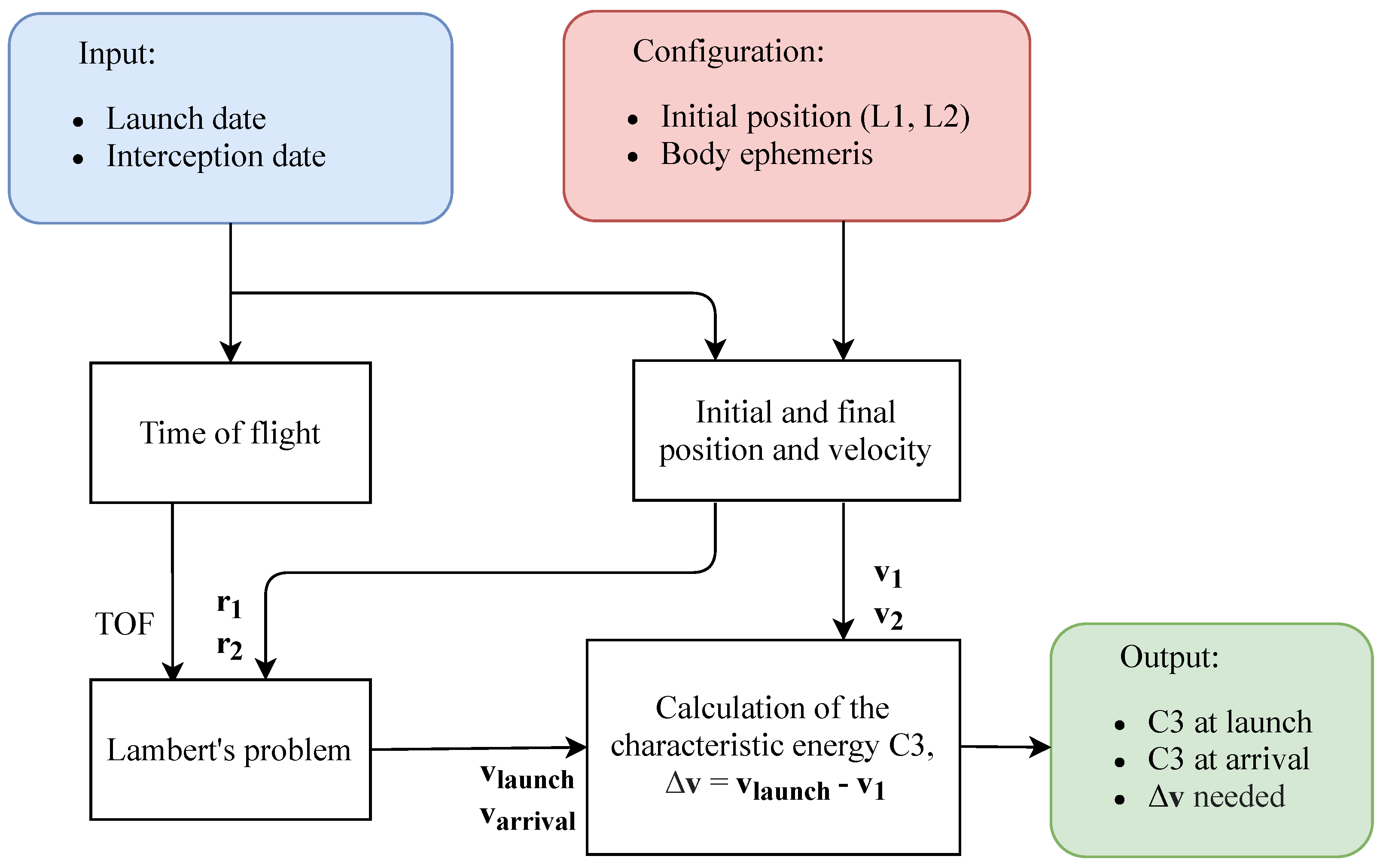
23]. This impulse is considered instantaneous and not necessarily coplanar. In our case, the launch date and the intersection date determine the initial and final positions. The difference between the initial velocity of this trajectory and the velocity carried by the interceptor in its original orbit corresponds to the impulse that must be applied to the vehicle to start its mission. The scheme followed for solving the Lambert’s problem is shown in
Figure 2. As the procedure is repeated for all possible combinations of launch and arrival dates, a porkchop plot is obtained, from which the optimal solution to the interception problem is extracted.
2.4. Iterative Correction of the Initial Impulse
Solutions to the Lambert’s problem define trajectories that reach a target position starting from an initial position with a fixed time interval. However, once perturbations are considered, the maneuver found by the simple Lambert’s problem does not allow us to obtain interception. The magnitude and direction of the impulse must therefore be readjusted until the approach of the launched vehicle becomes effective again. In order to accomplish this, an iterative scheme has been proposed to gradually modify the velocity impulse components until the relative distance of the two bodies is below a certain threshold, which is a parameter that depends on the nature of the mission.
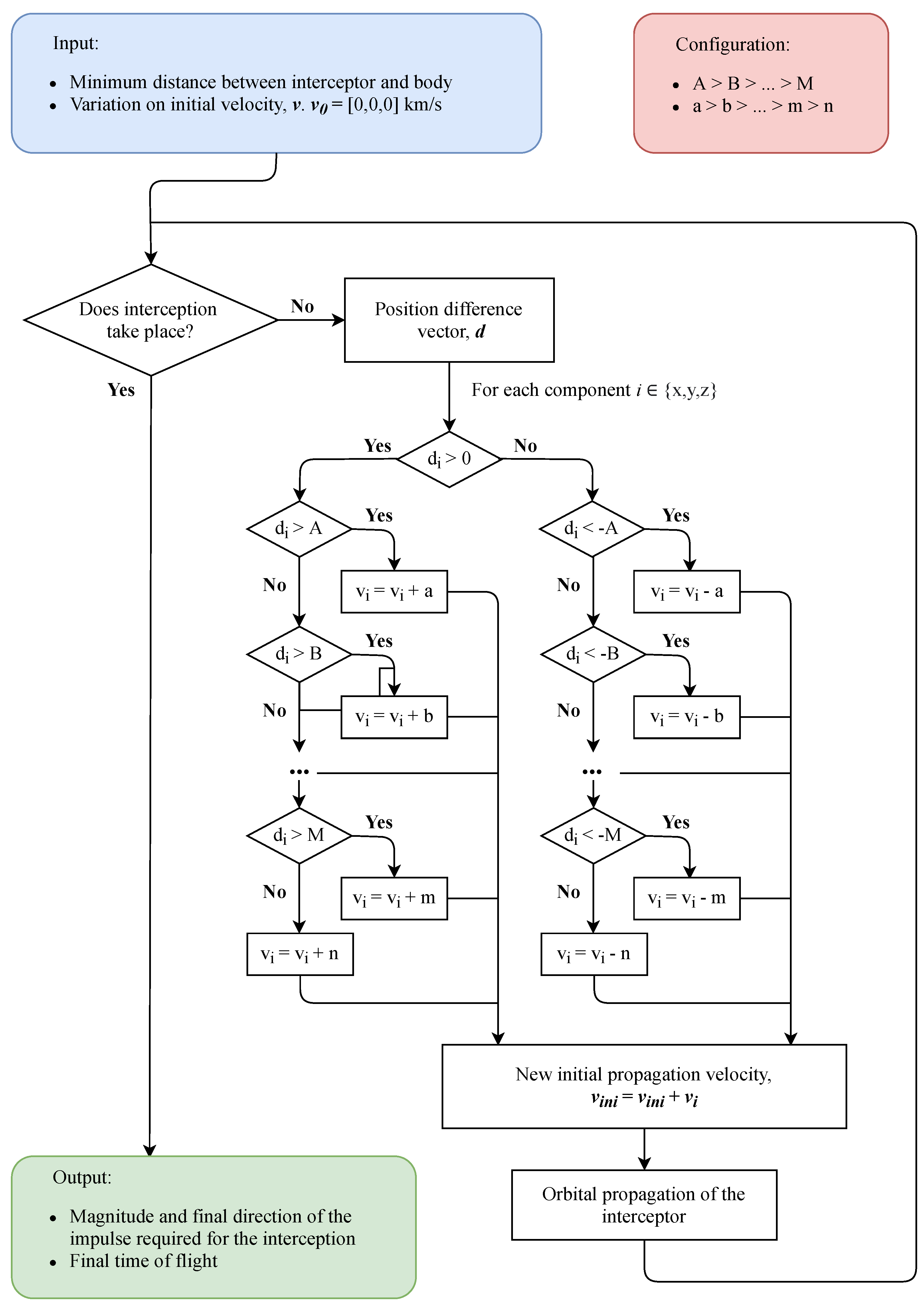
The method presented in this paper performs a correction on the impulse applied to the vehicle. This correction is proportional to the distance that separates both orbiters. Prior to the execution of the algorithm, a series of distance steps (A, B,…) and velocity corrections (a, b,…) are introduced. These values have been selected to progressively reduce the order of magnitude of both variables, but their choice can be subject to a further optimization process to minimize the number of iterations. As can be seen in the flow chart (
Figure 3), if the distance between both bodies is greater than a given value (i.e., the radius of the capture orbit or the dimensions of the celestial body), the position difference vector is stored and each of its components is analyzed independently. Positive differences imply an increase in velocity while negative differences result on a decrease. Next, the magnitude of each component is compared with the distance values previously introduced, in decreasing order. Depending on the interval in which it is bounded, a correction value will be added to that component of the impulse. Therefore, the further down the diagram you go, the smaller the difference in position between the bodies and the smaller the correction applied. Once the new impulse is obtained, the interceptor is propagated again, repeating the procedure until the interception is effective.
3. Results and Discussion
In order to test the tool, a realistic application case has been implemented: the interception of ’Oumuamua. An early detection of ’Oumuamua is assumed on 1 June 2017, when it was approaching the perihelion of its orbit. The interception window extends until December 2017. The integration time step has been set at 10 min, and it is assumed that an interceptor vehicle is available at both Earth–Sun Lagrange points L1 and L2, waiting to be launched. As for the sources of perturbation, the gravitational effects of all inner planets of the Solar System plus Jupiter and Saturn, as well as the SRP, are considered. The values of the radiation pressure coefficient and the area-to-mass ratio of ’Oumuamua have been obtained through a process of minimizing the errors between the state vector provided by the propagator and the one from HORIZONS [
31], as can be seen in
Table 1, recalling that it underwent non-gravitational accelerations whose origin has not yet been clarified. For the interceptor these values are
and
= 2 m
/kg, which are within the range commonly used for spacecrafts [
22,
28].
3.1. Keplerian Propagation of the ’Oumuamua
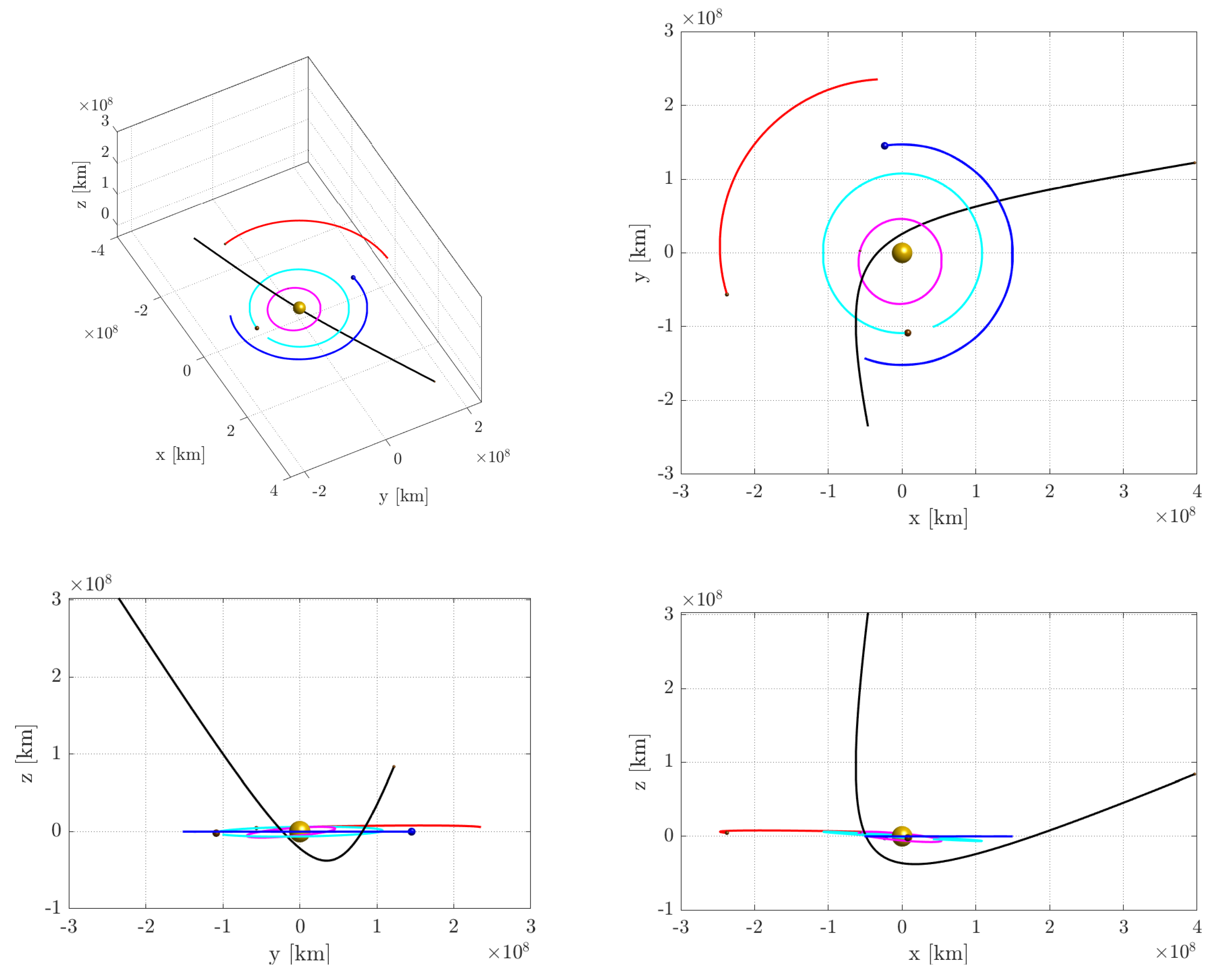
Firstly, a Keplerian propagation of the extrasolar object is performed, using the initial conditions given in
Table 1. This propagation is shown in
Figure 4, where the passage through the perihelion of ’Oumuamua has been captured.
The closest approach to Earth occurred on 14 October 2017, at 16:50 TDB. The distance between the Earth and the ’Oumuamua is approximately km (≈0.16 AU). Data from observations concluded that the closest passage occurred actually on 19 October, when ’Oumuamua passed at a distance of 0.16 AU. Note that, despite not taking perturbative phenomena into account, the results obtained for the Keplerian simulation are very close to the real ones. It does not differ significantly from the real trajectory, although it does differ in the instant it occupies each position in the orbit.
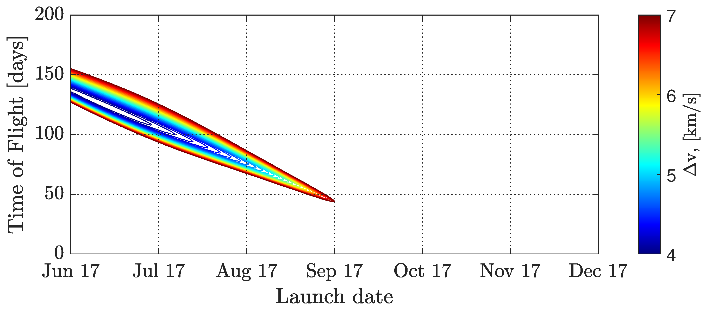
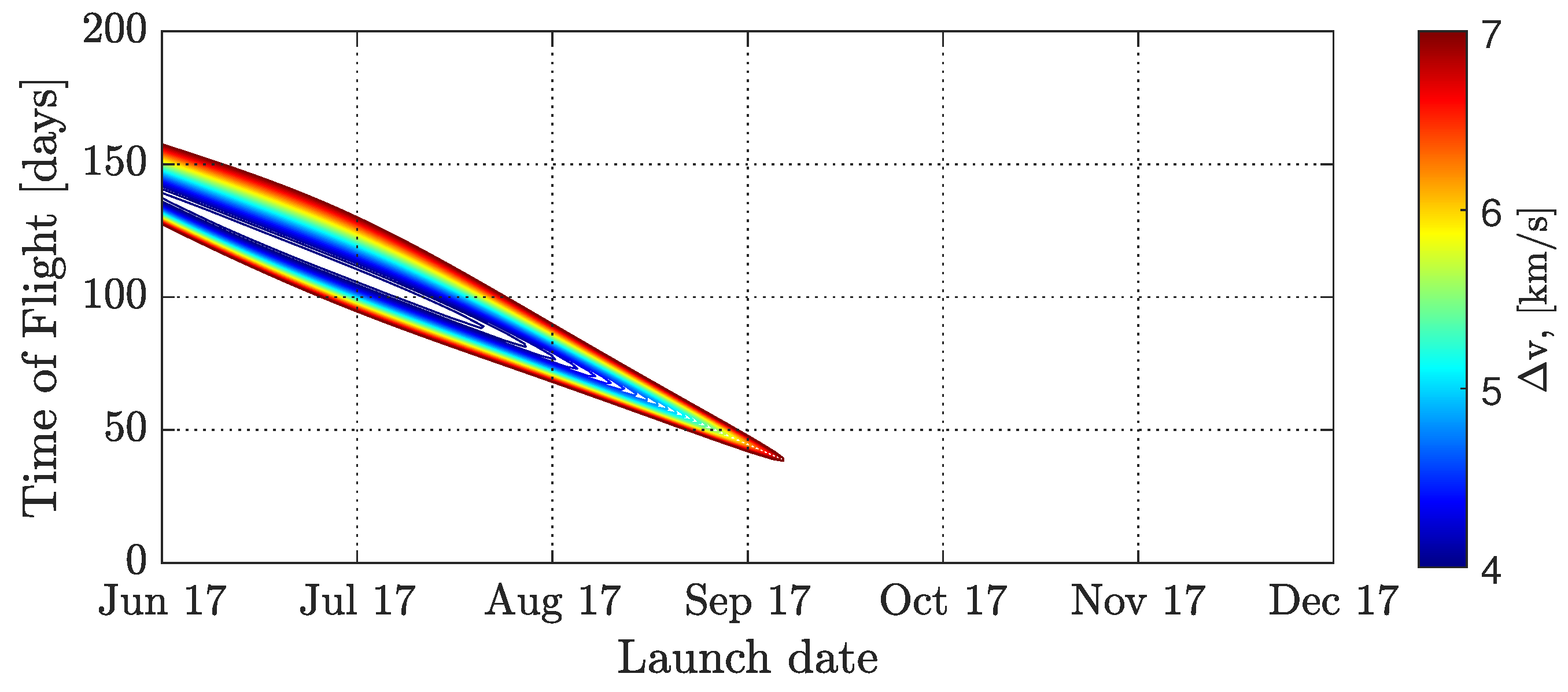
3.2. Determination of the Launch Porkchop Map of the Interceptor
The Keplerian orbit obtained in the previous phase allows us to solve the launch possibilities for intercepting ’Oumuamua, considering both Lagrange points L1 and L2 of the Earth–Sun system as possible starting points.
Following the scheme in
Figure 2 and after solving the factorial scheme for all possible combinations of launch and arrival dates from the two starting orbits, the porkchop plots for the obtained mission windows can be constructed.
Figure 5 and
Figure 6 show that the contour maps are very similar despite the starting point, L1 or L2. No maximum flight time has been set, unlike Seligman and Laughlin [
17], who set it at 90 days. Interception is therefore allowed to take place once the celestial body has made its closest approach to Earth. In addition, no parking orbit radius has been imposed for the arrival, as it is assumed that the dimensions of the celestial body are imprecise [
32,
33,
34,
35]. So, the interception will be considered fulfilled when the spacecraft goes 10 km near the target. Thus, the end point of the interception orbit will correspond to this position of the ’Oumuamua, although the tool allows the option of setting a distance at which to cease propagation, in order to initiate a possible capture maneuver.
The optimal trajectories that minimize the energy consumption of the maneuver for each of the launch orbits are listed in
Table 2. Based on the results obtained, a launch from the Lagrange point L2 is the best option since both the necessary impulse and the flight time are lower than those corresponding to the launch from L1. Moreover, the vehicle departure is 9 days later.
Note that the impulse values obtained and presented in
Table 2 are very similar to those given in [
17] and are energetically feasible.
3.3. Perturbed Propagation of the ’Oumuamua and the Interceptor Vehicle
A numerical integration is now carried out on the orbital model described in
Section 2.2, considering the aforementioned force distributions of the gravitational potentials of the inner planets of the Solar System, the most massive planets (Jupiter and Saturn) and the SRP. The Lagrange point L2 is taken as starting point for the interceptor vehicle (see
Table 3) and the initial conditions for the case of ’Oumuamua are those given in
Table 1. Additionally, the impulse obtained from the Lambert’s problem for the selected optimal trajectory is added to the velocity. In
Figure 7, the Keplerian and the perturbed solutions have been plotted for both bodies.
The representation in
Figure 7 shows the trajectory traveled up to the instant at which the distance between the two bodies is minimal. In the case of the Keplerian propagations, this distance becomes zero (the interception occurs), thus verifying that the solution of Lambert’s problem is correct. This ideal situation occurred on 17 October 2017.
When adding the effects of perturbations, the minimum distance between the two bodies is km (≈0.00857 AU), and it takes place on 16 October 2017 at 14:20 TDB. Clearly, in this case the interception does not occur since the ’Oumuamua orbit is more delayed than the Keplerian one and the interceptor trajectory is significantly displaced. So, it is necessary to correct the impulse applied to the interceptor vehicle.
In this way, and following the scheme presented in
Figure 3, the trajectory of the vehicle is recalculated modifying the
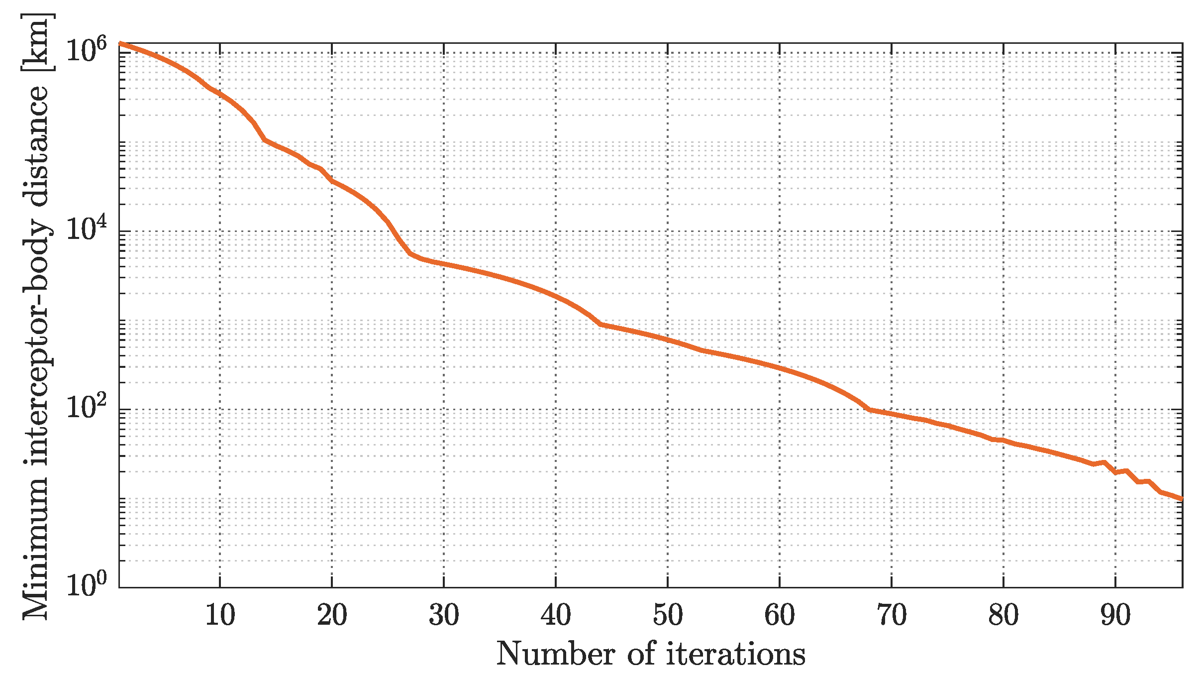
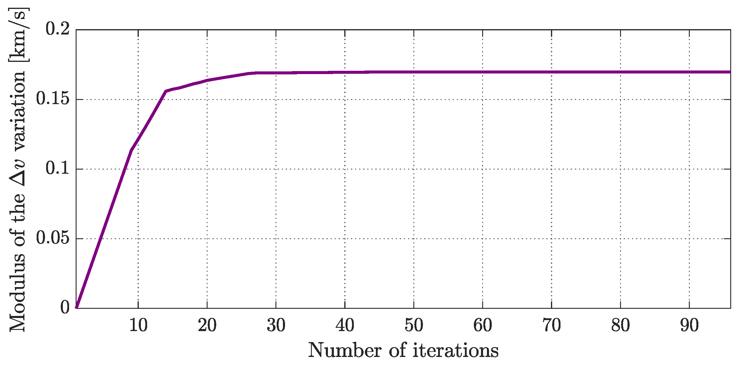
applied on its starting orbit. The iterative process has been set to end when the vehicle approaches within 10 km of the ’Oumuamua. It has been designed in such a way that the corrections made are variable depending on the magnitude of the distance to be covered. Therefore, in the first iteration, corrections of greater magnitude are made to achieve a considerably faster approach of the vehicle to its target, but as the distances become smaller, the corrections made are smaller, and this is reflected in
Figure 8 and
Figure 9: the minimum distance between the orbits of the ’Oumuamua and the interceptor after each iteration is shown in
Figure 8 and the magnitude of the velocity variation applied in each iteration over the initial propagation velocity is shown in
Figure 9. Note that the initial propagation velocity is the sum of the original velocity in the Lagrange point and the optimal impulse extracted from Lambert’s problem. It can be seen that, although the distance between the two bodies continues decreasing with each iteration, the variation of the modulus of the momentum stabilizes around 0.17 km/s before reaching the 30th iteration. This is justified by the fact that although the modulus seems invariant, there are still changes in the impulse components that mainly affect its direction, which have a noticeable effect in reducing the distance between the two bodies, as shown in
Figure 8. Therefore, the iterative process must continue to ensure that the interception takes place.
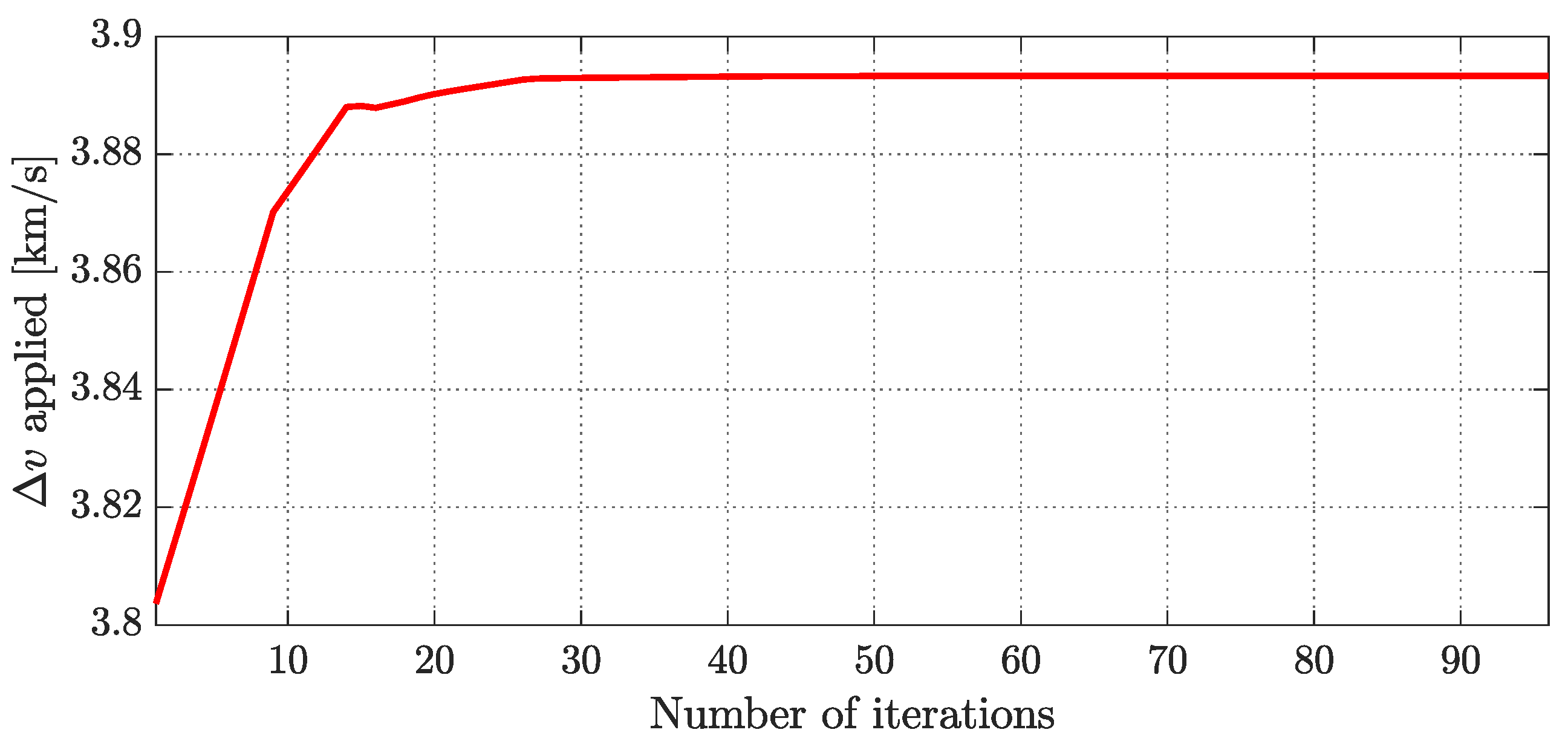
Figure 10 shows the evolution of the impulse applied on the initial conditions of the vehicle, i.e., the modification made on the orbital velocity it carries over the L2 point. The ideal solution of Lambert’s problem imposed an impulse of 3.8036 km/s, which corresponds to the initial value of the plot. After gradually modifying the three components of this impulse, it is concluded that an impulse of 3.8933 km/s is required. It should be recalled that although the figure only shows the evolution of the modulus of this impulse, its direction has also been corrected.
Finally, the evolution of the TOF is not a restrictive variable in this case, but it is useful to know it and to check if, when considering the corrections made, the interception takes place significantly earlier or later.
In fact, it can be checked that temporal changes are minimal. Initially, Lambert’s problem estimated the interception of ’Oumuamua on 17 October 2017, but the closest point between the two bodies prior to the impulse correction (see
Figure 7) took place on 16 October 2017 at 14:20 TDB, after a TOF of 117.6 days. Our tool, after correcting the trajectory, sets up the interception to take place on the same day, 16 October 2017 at 23:30 TDB, increasing slightly the TOF to 117.98 days. The vector state of both bodies at this instant can be seen in
Table 4.
Results of the problem in terms of the interceptor velocities are presented in
Table 5. A comparison between the interceptor velocities obtained in the ideal case (Lambert) and in the perturbed one shows that the variations can have considerable long-term effects on the trajectory of the vehicle, thus making it possible to cover the distance separating it from the celestial body to be intercepted. Discounting the velocity of the orbit followed by the vehicle at point L2, the components of the energy impulse to be applied by means of the propulsion methods available to the interceptor are determined. Finally, the modulus of this impulse is collected, with both results differing by less than 0.1 km/s.
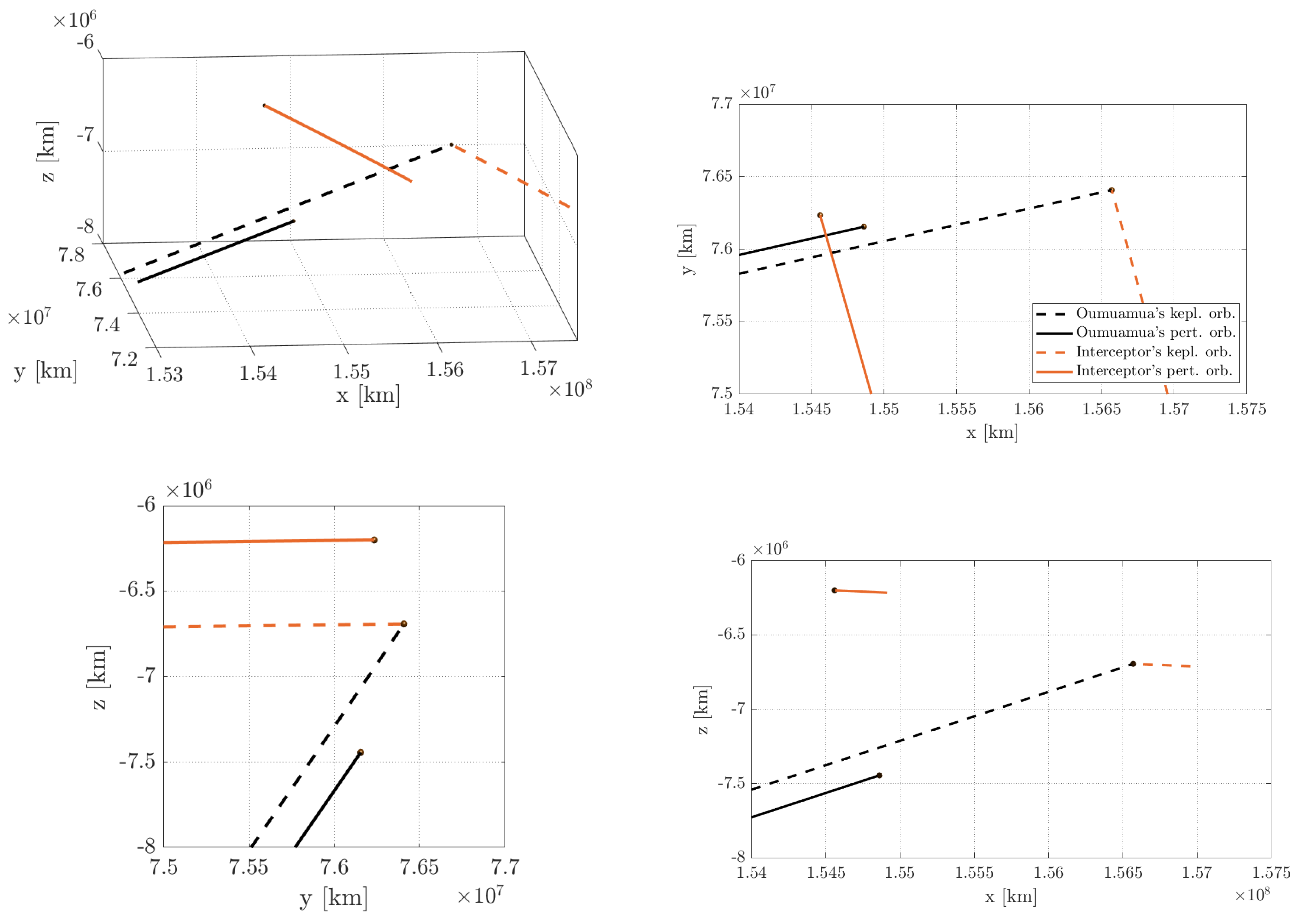
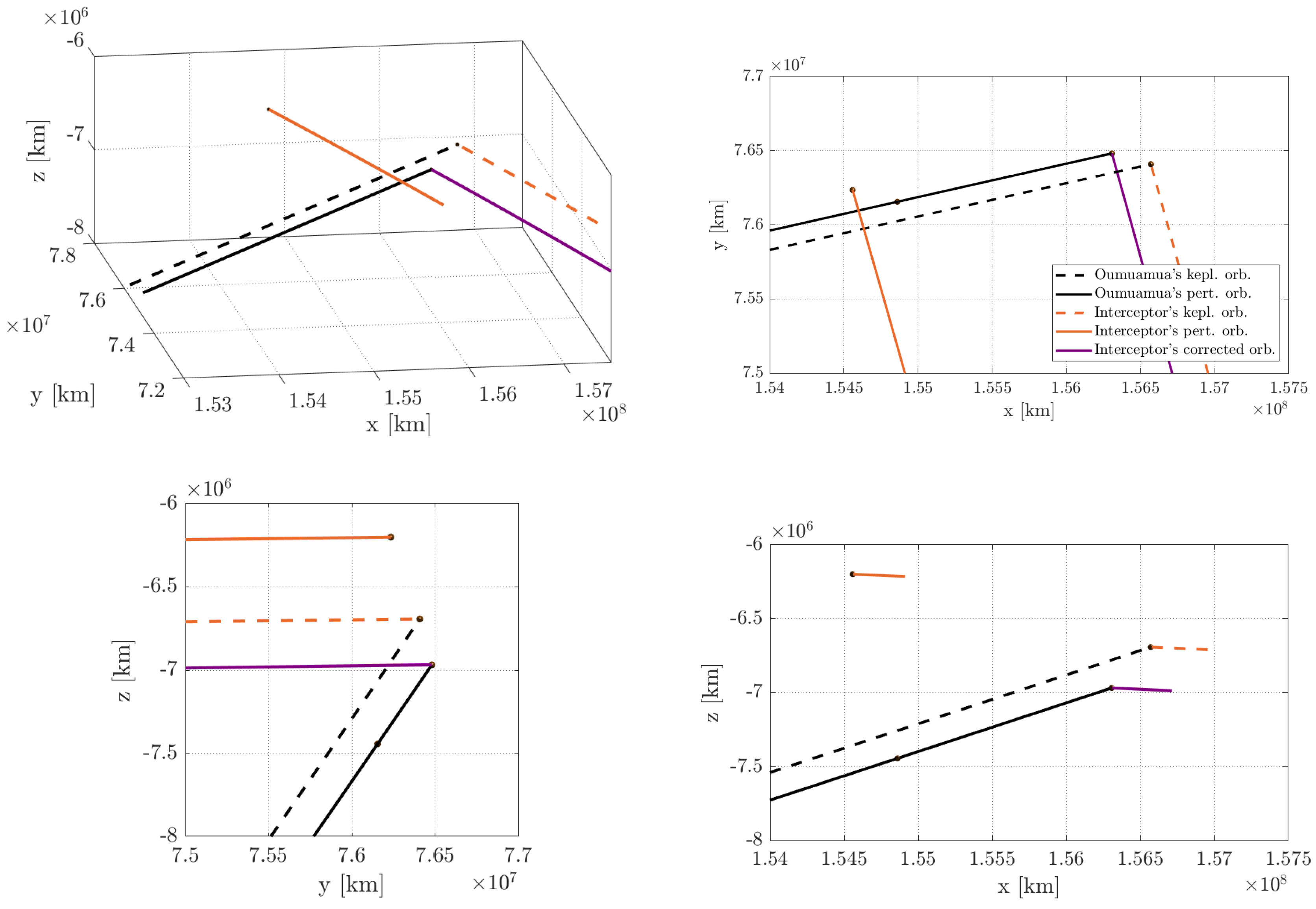
In the same way that the results prior to the correction have been represented, the trajectories followed by both bodies before the interception becomes effective are plotted in
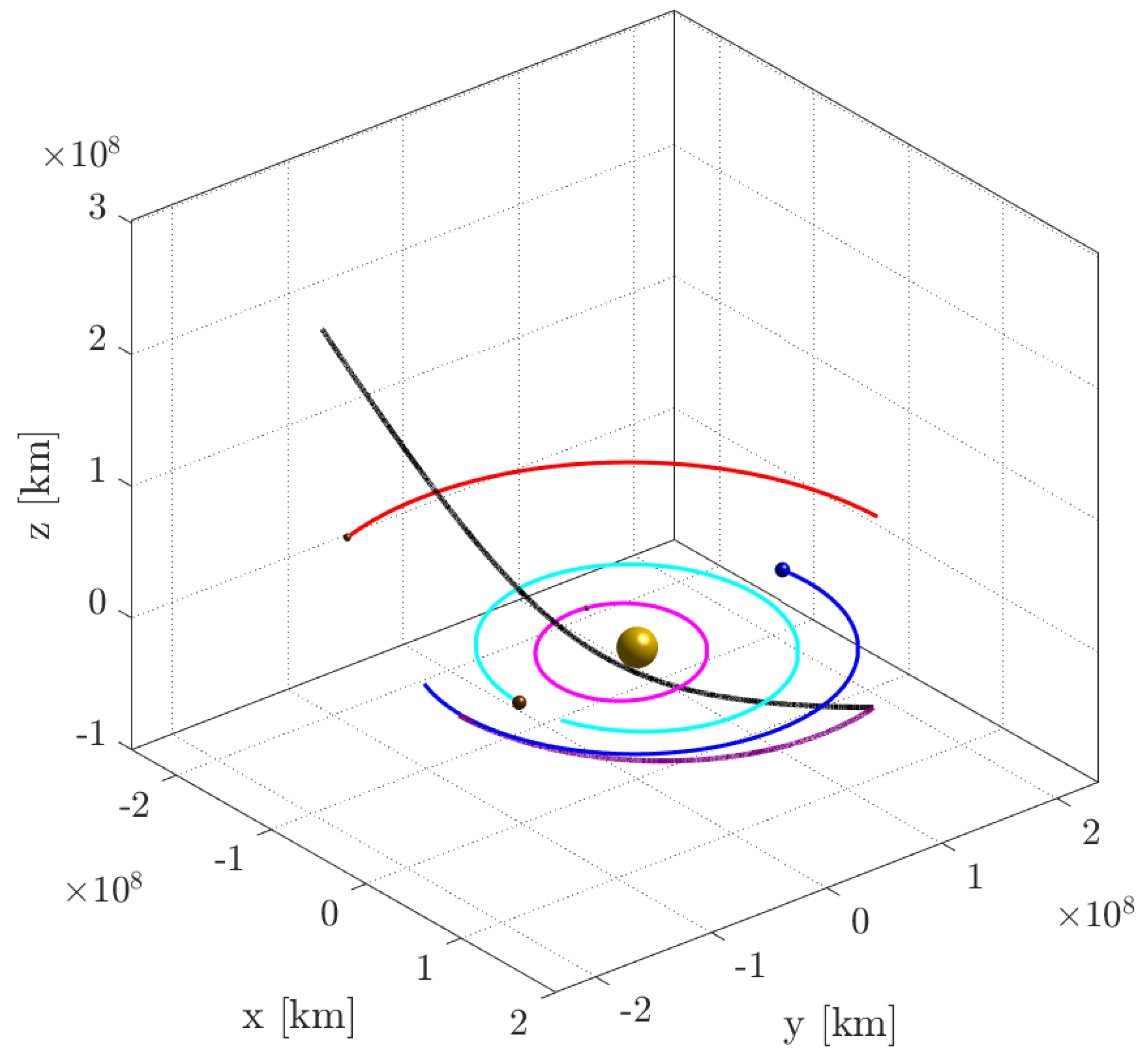
Figure 11. The final orbit of the interceptor has been significantly modified towards the ideal case. Meanwhile, the position of ’Oumuamua on its perturbed orbit has also changed. A three-dimensional representation of the final trajectories can be seen in
Figure 12.
4. Conclusions
In this paper, a study of interception maneuvers towards extrasolar bodies has been presented. Lambert’s problem has been solved to determine the interception trajectory that minimizes the energy cost of the mission extending the model of Seligman and Laughlin [
17] by introducing different perturbations on both the extrasolar object and the interceptor spacecraft. Moreover, the vehicle is located at one of the Lagrange points of the Earth–Sun system at launch instead of in an Earth orbit. An iterative process has been elaborated to correct the direction and magnitude of the impulse applied on the interceptor to ensure the interception of the extrasolar body.
The application case for intercepting the interstellar object ’Oumuamua in case of early detection has tested the study and yielded promising results. The resolution of Lambert’s problem has given similar results to those provided by Seligman and Laughlin [
17]. In this case, the required
is 3.8036 km/s with a launch from point L2 on 21 June 2017, and a mission time of 118 days.
The introduction of perturbations caused the solution extracted from Lambert’s problem to be no longer valid, with the minimum distance between the two bodies being km (≈0.00857 AU). However, after applying the iterative process of correction of the impulse, it has been ensured that the interception is once again effective, with the magnitude of the final being 3.8933 km/s, slightly higher than before, and the flight time practically identical, delaying the arrival of the vehicle to the target by a few hours.
The resolution of this case shows the ability of the presented tool to determine and correct the optimal trajectory of interception to bodies of extrasolar origin starting from the vicinity of the Lagrange points L1 or L2.


