Multi-Objective and Multi-Phase 4D Trajectory Optimization for Climate Mitigation-Oriented Flight Planning

Abstract

Aviation contribution to global warming and anthropogenic climate change is increasing every year. To reverse this trend, it is crucial to identify greener alternatives to current aviation technologies and paradigms. Research in aircraft operations can provide a swift response to new environmental requirements, being easier to exploit on current fleets. This paper presents the development of a multi-objective and multi-phase 4D trajectory optimization tool to be integrated within a Flight Management System of a commercial aircraft capable of performing 4D trajectory tracking in a Free Route Airspace context. The optimization algorithm is based on a Chebyshev pseudospectral method, adapted to perform a multi-objective optimization with the two objectives being the Direct Operating Cost and the climate cost of a climb-cruise-descent trajectory. The climate cost function applies the Global Warming Potential metric to derive a comprehensive cost index that includes the climate forcing produced by CO₂ and non-CO₂ emissions, and by the formation of aircraft-induced clouds. The output of the optimization tool is a set of Pareto-optimal 4D trajectories among which the aircraft operator can choose the best solution that satisfies both its economic and environmental goals.

1. Introduction

Air traffic provides a significant contribution to anthropogenic global warming. In 2005, aviation contributed about 5% of the overall anthropogenic radiative forcing (RF), with the largest warming contributions being due to CO₂ emissions, contrail cirrus formation, and NO_X net effects [1]. It is possible to reduce the environmental impact of aviation by intervening at the Air Traffic Management (ATM) level. The Single European Sky ATM Research (SESAR) framework has introduced the concept of Free Route Airspace (FRA) that allows the free planning of a route between any defined entry and exit point in the airspace, enabling shorter routes and a more efficient use of the airspace [2].

A partial implementation of the FRA concept in the European airspace from 2014 to 2018, limited to the upper airspace (above FL335 [3]) and to a portion of the European airspace, with 20% of flight time flown in free routing in 2017, produced an estimated saving of 2.6 million tons of CO₂ [4]. Current flight planning in FRA sections is limited to a reduction of route track path distance, and aims to reduce route extension (RE), i.e., the difference between flight and great circle distance between two waypoints. A full implementation of FRA will further reduce economic and environmental costs by enabling the definition of 4D flight profiles during flight planning, to be optimized with up-to-date weather information to define wind-optimal lateral paths and vertical profiles that exploit cruise climb techniques in lieu of cruise at level flight [5]. In this context, airborne trajectory optimization functionalities integrated within avionic systems will be a cornerstone of the network-centric ATM that will reduce Air Traffic Control (ATC) workload during flight plan definition [6].

1.1. 4D Trajectory Optimization

The trajectory optimization problem can be formulated as an Optimal Control Problem (OCP), commonly solved using numerical methods. The main approaches used to numerically solve OCPs are direct methods, indirect methods, and dynamic programming methods [7,8]. Direct methods are extensively used for aircraft trajectory optimization since they are easier to apply than indirect methods that require the derivation of the analytical expressions of the necessary conditions [7], and more efficient than classical dynamic programming methods that suffer from the “curse of dimensionality” and require the use of expert knowledge to reduce the solution search space [9,10]. In particular, direct collocation pseudospectral methods are characterized by a fast convergence to the optimal solution [11], and can be used to solve multi-phase problems [12,13]. Multi-phase optimization allows the optimization of an entire trajectory, composed of different flight phases corresponding to different aircraft modes and configurations that lead to a variation of the dynamic model [14,15]. Direct methods are at the base of many commercial off-the-shelf and general-purpose optimization tools [16,17,18]. However, when integrating 4D trajectory optimization functionality within the Flight Management System (FMS) of an aircraft, it is preferable to have a customizable and dedicated tool over a black-box solution.

The 4D trajectory optimization tool developed in this study will be integrated in the FMS of a Boeing 747-100, implemented in the Multipurpose Aircraft Simulation Laboratory (MASLab) developed within the Clean Sky research program, and able to execute 4D trajectory tracking [19,20,21]. The mathematical model of the aircraft used in the optimization tool uses Eurocontrol’s base of aircraft data (BADA) family 3 performance model for the propulsion system [22], while the aerodynamic model is based on Boeing 747-100 data gathered by Hanke and Nordwall [23]. The optimization algorithm is based on the Chebyshev pseudospectral direct method presented by [24], modified to allow sequential multi-phase optimization through a set of continuity boundary conditions of the states between phases and an estimation of the trajectory cost of subsequent phases in the cost function. The initial guess of the optimization algorithm is generated automatically: it is based on the orthodrome trajectory, flown at maximum specific range configuration with the respect to cost function that links the initial and final waypoints of the flight arc provided in input by the user. The optimization tool performs multi-objective optimization, using a weighted squared sum method, where the two conflicting objectives are the Direct Operating Cost (DOC) and the environmental cost of the trajectory.

1.2. Climate Mitigation-Oriented Flight Planning

Currently available 4D flight planning solutions offer the possibility to optimize routes with respect to fuel consumption, operating costs or flying time [25]. Fuel-optimal trajectories guarantee minimum CO₂ emissions; however, this does not imply a minimization of the environmental impact. In fact, CO₂ is the main contributor to anthropogenic global warming [26], yet the largest net warming effect produced by aviation is due to persistent contrails and contrail cirri, i.e., aviation-induced clouds (AIC), followed by CO₂ and NO_X [27]. In particular, 66% of the aviation net equivalent radiative forcing (ERF) in 2018 is due to non-CO₂ aviation climate forcings [27]. The three major aviation environmental impacts are climate impact, noise pollution, and air quality [28]. Noise pollution and air quality are generally addressed during initial and terminal phases of flight, as well as in the ground phases, where the aircraft is closer to highly populated areas [29,30]. Climate impact, defined as the sum of CO₂ and non-CO₂ net warming effect produced by the aircraft along the trajectory, is mainly addressed during cruise phase. Moreover, cruise is typically the only phase of flight concerned by AIC, since they form in the ice supersaturated regions (ISSR) of upper airspace [31]. For this reason, much research work focused on the reduction of AIC formation during cruise [32,33,34,35,36], facing the problem of a trade-off between contrail formation and the increased fuel consumption (with the ensuing increase in CO₂ emissions) necessary to avoid ISSRs. Other studies developed climate cost functions that exploit CO₂-equivalency metrics based on the ERF of aviation climate forcings to aggregate CO₂ and non-CO₂ net warming contributions into a single environmental cost index, in order to assess the mitigation potential of climate-optimal trajectories in the commercial airspace and their cost when compared to fuel-optimal trajectories [37].

This paper presents the development of a novel trajectory optimization tool for an effective climate mitigation-oriented 4D flight planning. Climate cost has been assumed as the environmental cost index that is provided as a choice among the other traditional cost indexes to be minimized during the definition of the flight plan (i.e., operating cost, fuel consumption, flight time). Multi-objective optimization with respect to DOC and environmental costs leads to a set of Pareto-optimal trajectories: in this way, it is possible to select, among multiple choices, the best flight plan that can satisfy both DOC and environmental goals of the aircraft operator. Multi-phase optimization allows the definition of the optimal climb-cruise-descent arc of the flight, i.e., the flight phases where it is possible to capitalize the benefits of FRA for climate mitigation. The environmental cost index is calculated in terms of CO₂-equivalent emissions of greenhouse gases (GHGs) and AICs produced by the aircraft during the climb-cruise-descent arc of the trajectory. The contributions of the individual climate forcings are weighted using the Global Warming Potential (GWP) emission metric integrated over a period of 20, 50, and 100 years [38]. Aircraft emissions are calculated using the Boeing Fuel Flow Method2 (BM2) [39], adopting engine-specific emission data from the International Civil Aviation Organization (ICAO) engine exhaust emissions databank [40]. Atmosphere and weather data are based on the Global Forecast System (GFS) model and provided by the National Oceanic and Atmospheric Administration (NOAA). The AIC formation model is built upon the Schmidt-Appleman criterion (SAC) for contrail formation, combined with a ISSR detection model [41]. The output of the multi-objective optimization tool is a set of Pareto-optimal 4D trajectories, i.e., a set of trajectories where each of the two objective costs, DOC and environmental cost, cannot be improved without worsening the other [42]. The extremes of the Pareto-optimal set of solutions are the DOC-optimal trajectory, with the higher environmental cost among the Pareto solutions, and the environmental-optimal trajectory, with the higher DOC.

The rest of the paper is organized as follows: Section 2 presents the trajectory optimization tool developed within this work, describing the optimization algorithm, the mathematical model of the aircraft, the atmospheric and AIC prediction model, the environmental cost model, the definition of the multi-objective cost function, the multi-phase optimization process, the initial guess trajectory generation; Section 3 shows the results for a test case based on a transatlantic flight from Rome to New York; Section 4 draws the conclusions about the work and suggests future improvements.

2. Materials and Methods

2.1. Direct Trajectory Optimization

The optimal trajectory is obtained performing a direct trajectory optimization using a Chebyshev pseudospectral method [24]. The trajectory optimization problem can be formulated as a general optimal control problem (OCP):

$$\begin{array}{cc}\hfill \underset{\mathit{x}\left(t\right),\mathit{u}\left(t\right),t_f}{min}& J[\mathit{x}\left(t\right),\mathit{u}\left(t\right),t]=M[\mathit{x}\left(t_f\right),t_f]+{\int }_{t_0}^{t_f}L[\mathit{x}\left(t\right),\mathit{u}\left(t\right),t]\mathrm{d}t\hfill \end{array}$$

(1a)

$$\mathrm{subject}\mathrm{to}:\{\begin{array}{}\hfill \mathrm{(1b)}& {\mathit{f}}_l\le \mathit{f}[\dot{\mathit{x}}\left(t\right),\mathit{x}\left(t\right),\mathit{u}\left(t\right),t]\le {\mathit{f}}_u\hfill \hfill \mathrm{(1c)}& {\mathit{b}}_l\le \mathit{b}[\mathit{x}\left(t_0\right),\mathit{x}\left(t_f\right),t_0,t_f]\le {\mathit{b}}_u\hfill \hfill \mathrm{(1d)}& {\mathit{c}}_l\le \mathit{c}[\mathit{x}\left(t\right),\mathit{u}\left(t\right),t]\le {\mathit{c}}_u\hfill \end{array}$$

where $\mathit{x}\left(t\right)$ and $\mathit{u}\left(t\right)$ are the states and control trajectories defined in the time $t\in [t_0,t_f]$. The solution of the OCP is given by the control function $\mathit{u}(·)$ and the corresponding trajectory $\mathit{x}(·)$ that minimize the Bolza cost function defined in (1a), and composed by the Mayer term $M(·)$ and the Lagrange term $L(·)$. The Problem (1) is subject to the dynamic constraints given in Equation (1b), the boundary constraints $\mathit{b}(·)$ in Equation (1c), and the algebraic path constraints $\mathit{c}(·)$ in Equation (1d).

Setting the lower and upper bounds equal to zero for the dynamic constraints in Equation (1b) leads to:

$$\mathit{f}[\dot{\mathit{x}}\left(t\right),\mathit{x}\left(t\right),\mathit{u}\left(t\right),t]=0$$

(2)

and assuming that the Jacobian $\partial \mathit{f}/\partial \dot{\mathit{x}}$ is nonsingular, the dynamic constraint can be represented by the controlled ordinary differential equation:

$$\dot{\mathit{x}}\left(t\right)=\mathit{f}[\mathit{x}\left(t\right),\mathit{u}\left(t\right),t]$$

(3)

The OCP may be solved using both direct or indirect solution methods: direct methods have the advantage of not needing to solve the necessary conditions derived from the Pontryagin maximum principle [24]. To apply direct methods, the OCP problem is discretized into a finite dimension nonlinear programming (NLP) problem: the domain of the independent time variable is subdivided into a finite number of intervals and the controls and states at the discretization points are evaluated through polynomial approximation. In direct collocation methods, both control and state variables at the nodes are the unknowns of the problem.

The Chebyshev pseudospectral method uses Chebyshev–Gauss-Lobatto (CGL) nodes as discretization points for the time variable. The CGL node points lie in the interval defined by the time domain $\tau \in [-1,1]$. Using a linear transformation, the problem is transformed from the generic interval $t\in [t_0,t_f]$ to $\tau \in [{\tau }_0,{\tau }_f]=[-1,1]$:

$$t\left(\tau \right)=\frac{(t_f-t_0)\tau +(t_f+t_0)}{2}$$

(4)

resulting in the following reformulation of the OCP in (1):

$$\begin{array}{cc}\hfill \underset{\mathit{x}\left(t\right),\mathit{u}\left(t\right),t_f}{min}& J[\mathit{x}\left(t\right),\mathit{u}\left(t\right),t]=M[\mathit{x}\left(1\right),t_f]+\frac{t_f-t_0}{2}{\int }_{-1}^{1}L[\mathit{x}\left(t\right),\mathit{u}\left(t\right),t\left(\tau \right)]\mathrm{d}\tau \hfill \end{array}$$

(5a)

$$\mathrm{subject}\mathrm{to}:\{\begin{array}{}\hfill \mathrm{(5b)}& {\mathit{f}}_l\le \mathit{f}\left[\frac{2}{t_f-t_0}\dot{\mathit{x}}\left(\tau \right),\mathit{x}\left(\tau \right),\tau \left(t\right),t\left(\tau \right)\right]\le {\mathit{f}}_u\hfill \hfill \mathrm{(5c)}& {\mathit{b}}_l\le \mathit{b}[\mathit{x}(-1),\mathit{x}\left(1\right),t_0,t_f]\le {\mathit{b}}_u\hfill \hfill \mathrm{(5d)}& {\mathit{c}}_l\le \mathit{c}[\mathit{x}\left(\tau \right),\mathit{u}\left(\tau \right),t\left(\tau \right)]\le {\mathit{c}}_u\hfill \end{array}$$

where for conciseness, $\mathit{x}\left(\tau \right)$ stands for $\mathit{x}\left[\tau \right(t\left)\right]$.

The $N+1$ CGL interpolation points are expressed in closed form as:

$${\tau }_k=-cos(\pi k/N),k=0,\dots ,N$$

(6)

Given the N-th order interpolating Chebyshev polynomials of the first kind, defined as:

$$T_j\left(\tau \right)=cos(jarccos\left(\tau \right)),j=0,\dots ,N$$

(7)

for $\tau \in [-1,1]$, which yields to

$$T_j\left({\tau }_k\right)=cos(\pi kj/N)$$

(8)

the interpolation points ${\tau }_k$ are the extrema of the interpolating polynomials, or the roots of their derivatives ${\dot{T}}_j\left(\tau \right)$.

The obtained CGL nodes are sorted in an ascending order and cluster in the proximity of the endpoints of the $[-1,1]$ interval, eliminating the Runge’s divergence for increasing values of N that occurs with equally spaced points [43].

The state and control continuous equations are obtained through polynomial approximation with the form:

$$\begin{array}{c}{\mathit{x}}^N\left(\tau \right)=\sum _{j=0}^N{\mathit{x}}_j{\varphi }_j\left(\tau \right)\end{array}$$

(9)

$$\begin{array}{c}{\mathit{u}}^N\left(\tau \right)=\sum _{j=0}^N{\mathit{u}}_j{\varphi }_j\left(\tau \right)\end{array}$$

(10)

where $\varphi \left(\tau \right)$ are Lagrange polynomials of order N interpolating function at the CGL nodes:

$${\varphi }_j\left(\tau \right)=\frac{{(-1)}^{j+1}}{N^2{c}_j}\frac{(1-{\tau }^2){\dot{T}}_N\left(t\right)}{\tau -{\tau }_j}$$

(11)

with

$$c_j=\left\{\begin{array}{c}2,j=0,N\hfill \\ 1,0<j<N\hfill \end{array}\right.$$

The interpolating polynomials show the Kronecker delta property:

$${\varphi }_j\left({\tau }_k\right)={\delta }_{jk}=\left\{\begin{array}{c}1,\mathrm{if}j=k\hfill \\ 0,\mathrm{if}j\ne k\hfill \end{array}\right.$$

The derivative of the states at the CGL node points can be expressed differentiating Equation (9):

$${\mathit{d}}_k={\dot{\mathit{x}}}^N\left({\tau }_k\right)=\sum _{j=0}^N{\mathit{x}}_j{\dot{\varphi }}_j\left({\tau }_k\right)=\sum _{j=0}^N{D}_{kj}{\mathit{x}}_j$$

(12)

where the differentiation matrix D is an expression in compact form of the Lagrange polynomials derivative and can be calculated as [44], adjusted for taking into account the ascending order of the interpolation points ${\tau }_k$:

$$\mathit{D}:=\left[D_{kj}\right]:=\{\begin{array}{c}\hfill \begin{array}{cc}\hfill \frac{c_k}{c_j}\frac{{(-1)}^{j+k}}{{\tau }_k-{\tau }_j},& j\ne k\hfill \\ \hfill -\frac{{\tau }_k}{2(1-{\tau }_k^2)},& 0<j=k<N\hfill \\ \hfill -\frac{2N^2+1}{6},& j=k=0\hfill \\ \hfill \frac{2N^2+1}{6},& j=k=N\hfill \end{array}\end{array}$$

(13)

The definite integral term of the continuous cost function can be discretized by approximating it to a finite sum using the Clenshaw–Curtis quadrature scheme. For a given function g:

$${\int }_{-1}^{1}g\left(\tau \right)\mathrm{d}\tau \approx \sum _{k=0}^{N}g\left({\tau }_k\right)w_k$$

(14)

where $w_k$ are the optimal quadrature weights and can be calculated as follows [45]:

$$w_k=\frac{c_k}{N}\left[1-\sum _{j=1}^{\lfloor N/2\rfloor }\frac{b_j}{4j^2-1}cos\left(\frac{2jk\pi }{N}\right)\right],k=0,\dots ,N$$

(15)

where the floor function $\lfloor N/2\rfloor$ returns an integer for any value of N and the coefficients $b_j$ and $c_j$ are defined as:

$$b_j=\left\{\begin{array}{c}1,j=N/2\hfill \\ 2,j<N/2\hfill \end{array}\right.,c_k=\left\{\begin{array}{c}1,k=0,N\hfill \\ 2,0<k<N\hfill \end{array}\right.$$

(16)

Equation (15) holds for any $N>1$.

The OCP is finally approximated as follows:

$$\begin{array}{cc}\hfill \underset{\mathit{X},\mathit{U},t_f}{min}& J[\mathit{X},\mathit{U},t_f]\approx M[{\mathit{x}}_N,t_f]+\frac{t_f-t_0}{2}\sum _{k=0}^{N}L[{\mathit{x}}_k,{\mathit{u}}_k,t_k]w_k\hfill \end{array}$$

(17a)

$$\mathrm{subject}\mathrm{to}:\{\begin{array}{}\hfill \mathrm{(17b)}& {\mathit{f}}_l\le \mathit{f}\left[\frac{2}{t_f-t_0}{\mathit{d}}_k,{\mathit{x}}_k,{\mathit{u}}_k,t_k\right]\le {\mathit{f}}_u,k=0,\dots ,N\hfill \hfill \mathrm{(17c)}& {\mathit{b}}_l\le \mathit{b}[{\mathit{x}}_0,{\mathit{x}}_N,t_0,t_N]\le {\mathit{b}}_u\hfill \hfill \mathrm{(17d)}& {\mathit{c}}_l\le \mathit{c}[{\mathit{x}}_k,{\mathit{u}}_k,t_k]\le {\mathit{c}}_u,k=0,\dots ,N\hfill \end{array}$$

where the coefficients

$$\mathit{X}=({\mathit{x}}_0,{\mathit{x}}_1,\dots ,{\mathit{x}}_N),\mathit{U}=({\mathit{u}}_0,{\mathit{u}}_1,\dots ,{\mathit{u}}_N)$$

and the final time $t_f$ are the unknown of the OCP that minimize the cost function, and are found using interior-point methods for NLP.

2.2. Aircraft Model

2.2.1. State Equations

The mathematical model of the aircraft is based on a conventional three degrees-of-freedom (3-DoF) rigid-body model with variable point-mass, expressed as a set of differential algebraic equations (DAE). The model is formulated assuming that the aircraft flies on the optimal trajectory in steady wings-level flight, adjusting the lateral path through steady turning flight with negligible turning rate, and performing major flight path level adjustments only during transitions to and from cruise with a negligible pull-up rate. The resulting 3-DoF flight dynamics DAE is given by the following state equations:

$$\begin{array}{c}\dot{\lambda }=\frac{Vcos\gamma cos\psi +w_N}{R_E+h}\end{array}$$

(18)

$$\begin{array}{c}\dot{\varphi }=\frac{Vcos\gamma sin\psi +w_E}{(R_E+h)cos\lambda }\end{array}$$

(19)

$$\begin{array}{c}\dot{h}=Vsin\gamma \end{array}$$

(20)

$$\begin{array}{c}\dot{m}=-T·TSFC\end{array}$$

(21)

$$\begin{array}{c}\dot{V}=\frac{T-D}{m}-gsin\gamma \end{array}$$

(22)

Equations (18) and (19) are the equations of motion on the lateral plane for latitude $\lambda$ and longitude $\varphi$ of the World Geodetic System (WGS84), and $R_E=f\left(\lambda \right)$ is the radius of Earth as a function of the latitude. The $w_N$ and $w_E$ terms represent respectively the North and East components of wind speed and are a function of latitude, longitude and altitude h. Equation (20) is the vertical equation of motion as a function of the flight path angle $\gamma$. Equation (21) is a function of the thrust T and the thrust specific fuel consumption $TSFC$. Equation (22) is the state equation for the true airspeed V and is a function of thrust T and aerodynamic drag D.

The control variables of the OCP are the heading angle $\psi$, the flight path angle $\gamma$, the throttle $\Pi$ that controls the thrust: $T=f(\Pi )$.

2.2.2. Performance Model

The aerodynamic model of the aircraft is based on the one built by Hanke and Nordwall for the NASA Flight Simulator For Advanced Aircraft (FSAA) of the Boeing 747-100 [23]. The model interpolates gridded data to calculate the aerodynamic drag coefficient $C_D$ as a function of the lift coefficient $C_L$ and the Mach.

The lift coefficient $C_L$ is calculated as:

$$C_L=\frac{2mgcos\gamma }{\rho V^{2}S}$$

(23)

The propulsive model of the aircraft is based on performance data from Eurocontrol’s base of aircraft data (BADA), family 3 [22]. The throttle $\Pi$ controls the thrust $T\in [T_{idle},T_{max}]$ with the following linear law:

$$T(\Pi )=T_{idle}+\Pi (T_{max}-T_{idle})$$

(24)

where the minimum idle and maximum thrust available are a function of the flight conditions and BADA coefficients specific to the aircraft. The fuel flow $FF$ is then calculated as a function of the thrust and the thrust specific fuel consumption $TSFC$:

$$FF=T·TSFC$$

(25)

The $TSFC$ is defined in BADA as a function of engine-specific coefficients and true airspeed [22].

2.2.3. Emissions Model

Emissions are calculated to estimate the climate impact of the trajectory. The mass of a generic pollutant $m_{gp}$ emitted during a given flight time can be calculated as

$$m_{gp}={\int }_{t_0}^{t_f}FF·E{I}_{gp}\mathrm{d}t$$

(26)

where the $E{I}_{gp}$ is the emission index of the given pollutant and represents the mass of emission per mass of fuel burned. Emission indexes are available for carbon dioxide CO₂, water vapor H₂O, sulfur dioxide SO₂, soot, nitrogen oxides NO_X, unburned hydrocarbons HC, and carbon monoxide CO. The emissions indexes in

Table 1. Values of the constant emission indexes [27].

Emission	Emission Index (EI)
CO2	3.159 kg/kg fuel
H2O	1.231 kg/kg fuel
SO2	1.2 g/kg fuel
Soot	0.03 g/kg fuel

have been assumed to be constant throughout the trajectory, hence the mass of emission is proportional to the mass of fuel burned.

The emissions indexes of NO_X, HC, and CO vary as a function of the fuel flow and the atmospheric conditions and are calculated using the Boeing Fuel Flow Method2 (BM2) [39] using emissions data from the International Civil Aviation Organization (ICAO) engine exhaust emissions databank [40]. These data, provided to ICAO by the engine manufacturers, consist of coupled values of a relative emission index (REI) and a fuel flow factor $W_{FF}$ at four power settings, i.e., idle/taxi (7%), approach (30%), climb (85%), and take-off (100%).

The fuel flow factor $W_{FF}$ is defined as:

$$W_{FF}=FF\frac{{\vartheta }_{amb}^{3.8}}{{\delta }_{amb}}exp\left(0.2M^2\right)$$

(27)

where ${\vartheta }_{amb}$ and ${\delta }_{amb}$ are respectively the ratios between ambient temperature and pressure with respect to the sea level values.

Nonlinear regression with least square error can be applied to ICAO engine data to derive the following formulation of NO_X REI as a function of the fuel flow factor $W_{FF}$:

$$RE{I}_{N{O}_X}\left(W_{FF}\right)=6.5991·W_{FF}^2+3.1542·W_{FF}+2.5003$$

(28)

The emission index for NO_X can be finally obtained using the following relation:

$$E{I}_{N{O}_X}=RE{I}_{N{O}_X}·exp\left(H\right)·{\left(\frac{\delta {amb}^{1.02}}{{\vartheta }_{amb}^{3.3}}\right)}^{0.5}$$

(29)

where H is a humidity factor that depends on ambient pressure and relative humidity [39].

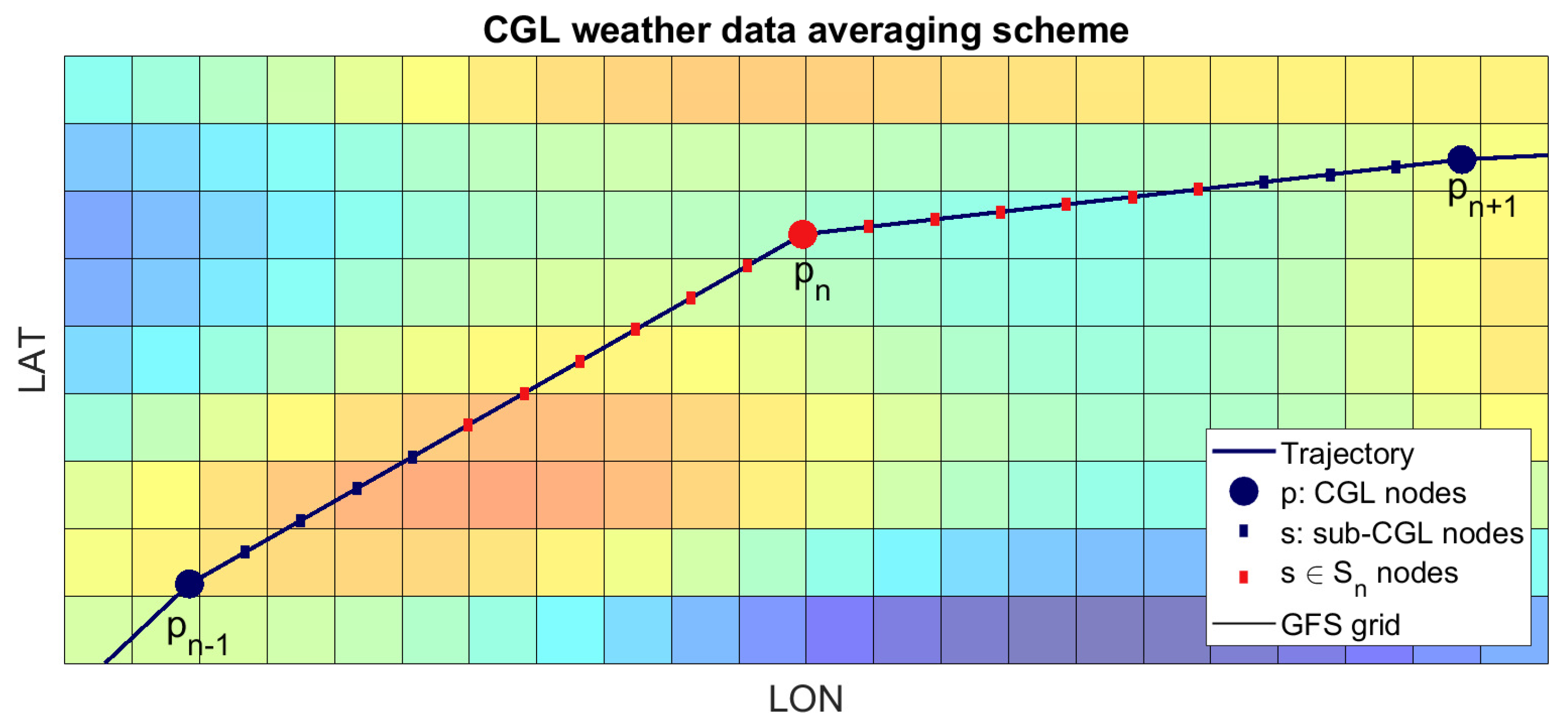
2.3. Atmosphere Model

Atmosphere data are provided by the National Oceanic and Atmospheric Administration (NOAA) through the NOAA Operational Model Archive and Distribution System (NOMADS) based on the Global Forecast System (GFS) model. Weather data are gathered in lookup tables with a base horizontal resolution of 0.25 degrees and a mean vertical pressure altitude resolution of 25 millibars. Gridded weather data downloaded from NOMADS are the north and west wind velocity components $w_N$ and $w_E$ in m/s, ambient temperature $T_{amb}$ in K, relative humidity $RH$ defined by values between 0 and 1.

Pressure altitude QNE expressed in meters h and ambient pressure p in Pascals are directly related as in [46]:

$$h=\left[1-{\left(\frac{p}{101325}\right)}^{0.190284}\right]·\mathrm{44,307.694}$$

(30)

The density for moist air ${\rho }_a$ is derived from the CIPM-2007 formula [47]:

$${\rho }_a=\frac{p{M}_a}{ZR{T}_{amb}}\left[1-x_v\left(1-\frac{M_v}{M_a}\right)\right]$$

(31)

where $M_a$ and $M_v$ are the molar masses of dry air and water vapor, $x_v$ is the molar fraction of water vapor, Z is the compressibility factor and R is the molar gas constant in J mol⁻¹ K⁻¹.

Sub-CGL Grid

The spatial resolution of the GFS data grid, equal to 0.25 degrees, has an order of magnitude of ∼${10}^1$ km, whereas the cruise phase of a long-haul flight spans over an arc with a length of ∼${10}^3$ km. Consequently, if the nodes of the CGL grid are lower than N∼${10}^2$ it means that the GFS grid resolution is higher than the CGL resolution used for pseudospectral optimization. In these cases, all the information about the atmospheric conditions between CGL nodes is lost. This problem is solved by creating a sub-CGL grid, with equidistant sub-nodes between CGL points that have a spatial resolution comparable to the one of the GFS grid, and lay on the geodesic trajectory that links consecutive CGL nodes, as shown in Figure 1. All the other state and control variables in the arcs between CGL nodes are approximated using linear interpolation.

The actual atmosphere variable $\overline{\omega }$ attributed to a specific CGL node in pseudospectral optimization is calculated as follows. Defining P the set of N + 1 CGL nodes p, and S the set of the M nodes s of the sub-CGL grid, $S_n$ is defined as the set of s nodes that are closer to a given $p_n$ node, with $p\in [0,N]$ than to any other CGL node. The atmosphere variable attributed to the $p_n$ CGL node is calculated by averaging the atmosphere GFS data for the coordinates of the nodes in the $S_n$ set of $|S_n|$ elements:

$${\overline{\omega }}_n=\frac{{\sum }_{i=1}^{|S_n|}\omega \left(s_i\right)}{|S_n|}$$

(32)

where $\omega$ is a generic atmospheric variable gathered from the GFS gridded data as a function of spatial coordinates of node $s_i$.

2.4. Aircraft-Induced Clouds Model

With the performance data of the aircraft model and the atmospheric model it is possible to detect the formation of persistent contrails and contrail cirri, to evaluate their impact in the environmental cost.

According to Schmidt-Appleman criterion (SAC) condensation trails form if the atmospheric temperature is lower than a threshold temperature $T_{LC}$ [41]. Short-lived contrails dissolve in seconds to a few minutes, with little impact on Earth’s radiative forcing. Contrails that last for at least 10 min are defined as persistent contrails by the World Meteorological Organization [48]. Persistent contrails only form and evolve in ice supersaturated regions (ISSR), where the relative humidity over ice RHi is greater than 100%:

$$R{H}_i=RH\frac{p_{liq}}{p_{ice}}$$

(33)

where $p_{liq}$ and $p_{ice}$ are the saturation pressures over liquid and ice water surfaces and can be calculated using the equations in [49].

Contrail cirri form when ISSR cold and moist conditions further influence the radiative properties of the persistent contrail, along with its shape, size, and duration, making them almost indistinguishable from natural ice clouds [31].

Persistent contrails and contrail cirri altogether are defined as aircraft-induced clouds (AIC), and form if both SAC and ISSR conditions are true:

$$\{\begin{array}{c}{T}_{amb}\le T_{LC}\hfill \\ R{H}_i=RH\frac{p_{liq}}{p_{ice}}\ge 1\hfill \end{array}$$

(34)

The threshold temperature for the SAC criterion $T_{LC}$ is calculated by applying the formulation in [41]:

$$T_{LC}=T_{LM}-(1-RH)\frac{p_{liq}\left(T_{LM}\right)}{G}-\Delta T_c$$

(35)

where all the temperatures are expressed in °C, $\Delta T_c$ is a correction factor that is equal to 0 for relative humidity $RH=\{0,1\}$ and positive otherwise; $T_{LM}$ is the maximum threshold temperature for $RH=1$ and is given by:

$$T_{LM}=-46.46+9.43ln(G-0.053)+0.72{[ln(G-0.053)]}^2$$

(36)

Finally, G is expressed in Pa K⁻¹ and is given by:

$$G=\frac{c_p{p}_{amb}E{I}_{H_{2}O}}{(M_v/M_a)Q_f(1-\eta )}$$

(37)

with specific heat capacity of air $c_p$ = 1004 J, $Q_f$ is fuel specific energy in J kg⁻¹, and $\eta$ is the overall propulsion efficiency of the aircraft.

2.5. Multi-Objective Cost Functional

2.5.1. Direct Operating Cost

The direct operating cost (DOC) is the monetary cost of the flight and is directly impacted by duration and fuel consumption:

$$J_{DOC}={\int }_{t_0}^{t_f}(C_t+FF·C_f)\mathrm{d}t$$

(38)

where $C_t$ is the estimated direct operating cost per unit time excluding fuel and $C_f$ is the cost of fuel per unit mass. The cost coefficients used within the optimization tool are based on data for the year 2018, and are $C_t$ = 0.5381 $/s [50], and $C_f$ = 0.7152 $/kg [51]. The DOC is the Mayer term of the cost function of the optimization problem as defined in Equation (1a), since $C_t$ and $C_f$ are constant, hence $J_{DOC}$ depends only on final time and states and can be rewritten as:

$$J_{DOC}=C_t(t_f-t_0)+C_f(m_f-m_0)$$

(39)

2.5.2. Environmental Cost

The environmental cost function is composed by the climate cost and measures the contribution of a given trajectory to global warming. Aviation contributes to anthropogenic global warming through the emissions of different greenhouse gases (GHGs) and other climate forcing agents such as AIC. Emission metrics have been introduced to compare the warming contribution of components with different physical properties and express them in a common unit, as CO₂-equivalent emissions [38]. The Global Warming Potential (GWP) measures how much energy the emission of 1 ton of a gas will absorb over a given time period, relative to the emission of 1 ton of carbon dioxide (CO₂). Varying the reference time horizon, e.g., 20, 50, or 100 years, affects the magnitude of the metric according to the atmospheric lifetime decay of the forcing agent. By definition, CO₂ has a GWP of 1 regardless of the time period used, since it is the gas being used as the reference. GWP is only one of various CO₂-equivalent emission metrics proposed in the literature, and the choice of one metric over the other depends on the environmental target that must be investigated (e.g., emission reduction target, temperature target).

For a given trajectory, the climate forcing agents produced by the aircraft (i.e., GHGs and contrail cirri) can be combined by means of a weighted sum, resulting in the environmental cost $J_{ENV}$:

$$J_{ENV}=\sum _{s=1}^{N_{species}}E{M}_s{\int }_{t_0}^{t_f}FF\left(t\right)·E{I}_s\left(t\right)\mathrm{d}t$$

(40)

where for each emission specie s, the weight $E{M}_s$ is given by the chosen emission metric from

Table 2. Global Warming Potentials of the climate forcings considered in the environmental cost function for time horizons of 20, 50, 100 years [27]. AIC values have been adjusted considering a global mean flight fraction with contrail formation of 15.6% [52], while values reported in [27] consider AIC based on global flight distance of flights scheduled in 2018.

Emission	GWP20	GWP50	GWP100
CO2	1	1	1
AIC (Tg CO2 basis)	14.87	6.99	4.04
AIC (km basis)	256	122	71
Net NOX	619	205	114
Soot	4288	2018	1166
SO2	−832	−392	−226
Water vapor	0.22	0.10	0.06

. The environmental cost is measured in CO₂-equivalent mass, since it is the result of the mass of the emission given by the integration term, as for Equation (26), multiplied by the CO₂-equivalent emission metric.

The value of the emission index of AIC, $E{I}_{AIC}=\{0,1\}$, equals 1 in the presence of AIC, according to Equation (34), and is null otherwise.

2.5.3. Multi-Objective Cost Function

A nontrivial multi-objective optimization problem that must minimize two or more conflicting objectives does not have a single solution that minimize each objective at the same time, but a set of optimal solutions defined as the Pareto-optimal set of solutions that lay on the Pareto front of the feasible solutions set in the objective space. For each solution in the Pareto-optimal set, it is not possible to further optimize one of the objectives without penalizing the others.

The multi-objective trajectory optimization is solved using a quadratic weighted sum method, where the multi-objective cost function of the OCP problem defined in Equation (17a) can be rewritten using the following scalar expression [53]:

$$J=w_{DOC}{\left(\frac{J_{DOC}}{{\sigma }_{DOC}}\right)}^2+w_{ENV}{\left(\frac{J_{ENV}}{{\sigma }_{ENV}}\right)}^2$$

(41)

where $w_{DOC}$ and $w_{ENV}$ are the weights attributed to each objective function, while ${\sigma }_{DOC}$ and ${\sigma }_{ENV}$ are scaling factors used to normalize the single objective costs with respect to a reference value.

Weights of the weighted sum method must satisfy the following conditions:

$$\{\begin{array}{c}{w}_{DOC},w_{ENV}\ge 0\hfill \\ w_{DOC}+w_{ENV}=1\hfill \end{array}$$

(42)

and their values are assigned using the following linear form:

$$\{\begin{array}{c}{w}_{DOC}=(1-\kappa )\hfill \\ w_{ENV}=\kappa \hfill \end{array},\kappa \in [0,1]$$

(43)

Shifting the value of the parameter $\kappa$ towards 0 increases the weight of $J_{DOC}$ in the optimization, producing trajectories with lower operating costs, while shifting $\kappa$ towards 1 increases the weight of $J_{ENV}$, producing greener trajectories. The squared weighted sum method consists of solving the optimization problem for several values of $\kappa$ to find a set of feasible trajectories and identify the Pareto set of optimal solutions.

The scaling factors ${\sigma }_{DOC}$ and ${\sigma }_{ENV}$ are respectively the DOC and the environmental cost of the minimum DOC trajectory, calculated by solving the OCP problem as defined in (17), with a single objective cost function consisting only in the Mayer term of Equation (17a) and corresponding to the definition of the DOC in Equation (39):

$$\underset{{\mathit{X}}_{DOC},{\mathit{U}}_{DOC},{t_f}_{DOC}}{min}{J}_{DOC}[\mathit{X},t_f]$$

(44)

where ${\mathit{X}}_{DOC}$ is the state vector of the DOC-optimal trajectory, ${\mathit{U}}_{DOC}$ the control vector, and ${t_f}_{DOC}$ the final time. The scaling factors ${\sigma }_{DOC}$ and ${\sigma }_{ENV}$ are then calculated using Equations (39) and (40):

$$\begin{array}{cc}\hfill {\sigma }_{DOC}& =J_{DOC}[{\mathit{X}}_{DOC},{\mathit{U}}_{DOC},{t_f}_{DOC}]\hfill \end{array}$$

(45)

$$\begin{array}{cc}\hfill {\sigma }_{ENV}& =J_{ENV}[{\mathit{X}}_{DOC},{t_f}_{DOC}]\hfill \end{array}$$

(46)

The weighted sum method is widely used given its simplicity; however, it has some issues that must be taken into account. The solution for a given $\kappa$ does not necessarily belong to the Pareto set in the objective space, and uniform spacing in $\kappa$ may not correspond to uniformed solutions in the objective space. Furthermore, the method only works with convex Pareto fronts. These issues can be mitigated by proper normalization of the objectives and by solving the problem using a high number of $\kappa$ values, to obtain a valid Pareto set of solutions. If these resolutions do not work, the problem may have a non-convex Pareto front and another multi-objective optimization method should be used.

2.6. Multi-Phase Trajectory Optimization

The optimization tool optimizes multi-phase trajectory composed by climb, cruise, and descent phases. The multi-phase optimization is performed sequentially, starting from the climb phase, and each phase is optimized individually. The following continuity boundary conditions are formulated to assure continuity of the aircraft states during phase changes at top-of-climb (TOC) and top-of-descent (TOD):

$$\begin{array}{c}{\mathit{x}}_0^{\left(cr\right)}={\mathit{x}}_N^{cl}\end{array}$$

(47)

$$\begin{array}{c}{\mathit{x}}_0^{\left(ds\right)}={\mathit{x}}_N^{cr}\end{array}$$

(48)

Discontinuity of the throttle control variable $\Pi$ is permitted, while the flight path angle $\gamma$ and the heading angle $\psi$ are constrained as the states.

To obtain an optimal climb-cruise-descent arc trajectory, the cost function of each phase must include an estimation of the costs of the subsequent phases, following the Bellman’s principle of optimality [54]. In other words, the optimal climb trajectory is not the one with the minimum climb cost, but the one that produces the optimal climb-cruise-descent trajectory with the overall minimum cost. Prior to each phase optimization, the initial guess (IG) trajectory is automatically calculated by propagating the aircraft conditions at the initial waypoint WP of the given phase, assuming an aircraft configuration that guarantees the maximum specific range (SPR) along the geodesic trajectory that leads to WP2.

Inputs for the optimization problems are the start-of-climb (SOC) and end-of-descent (EOD) coordinates and altitude, defined respectively as WP1 and WP2, the initial mass of the aircraft $m_0$, the time at SOC. TOC and TOD waypoints are obtained through the optimization process. The optimal trajectory is performed assuming a free route airspace (FRA) between WP1 and WP2, with continuous climb and descent operations (CCO and CDO), and idle descent. The optimization procedures for each phase are described in the following subsections.

2.6.1. Climb Phase

Climb Phase Cost Function

Climb is the first phase to be optimized, and the cost function of the optimal climb needs to also include the approximated costs of cruise and descent phases. The cost function to be minimized for the climb phase is defined as follows:

$$J=J_{cl}[{\mathit{X}}^{\left(cl\right)},{\mathit{U}}^{\left(cl\right)},t_f^{\left(cl\right)},\kappa ]+{\tilde{J}}_{cr}+{\tilde{J}}_{ds}$$

(49)

where $J_{cl}$ is the actual cost of the climb trajectory as defined in Equation (17a)

$$J_{cl}=J[{\mathit{X}}^{\left(cl\right)},{\mathit{U}}^{\left(cl\right)},t_f^{\left(cl\right)},\kappa ]$$

(50)

and is a function of the climb state and control variables, of the final time of climb $t_f^{\left(cl\right)}$, and of the multi-objective coefficient $\kappa$. The subscript ${}^{\left(cl\right)}$ indicates variables of the climb phase, ${\tilde{J}}_{cr}$ and ${\tilde{J}}_{ds}$ are the approximated costs of the cruise and descent phases.

The cost of the approximated descent phase ${\tilde{J}}_{ds}$ can be considered to be negligible when compared to cruise and climb cost, since with idle descent $F{F}_{ds}\approx 0$.

The cost of the approximated cruise phase ${\tilde{J}}_{cr}$ can be estimated by making the following assumptions:

(i)

the lateral path of the approximated cruise lays on the geodesic curve that links the TOC to WP2 (i.e., minimum distance lateral path);

(ii)

the TOD of the approximated cruise corresponds to WP2 since for long-haul flights the descent track path distance is negligible when compared to cruise distance, hence ${\tilde{J}}_{cr}{{|}_{TOC\to WP2}\approx {\tilde{J}}_{cr}|}_{TOC\to TOD}$. This assumption allows the avoidance of the estimation of the TOD for each iteration of the cost function;

(iii)

the vertical path and the true airspeed of the aircraft for each point in the cruise trajectory are such that the SPR is maximized. Hence:

$$\underset{V,h}{max}SPR\left(\kappa \right)=\frac{d_{cr}}{J_{cr}\left(\kappa \right)}$$

(51)

where $d_{cr}$ is cruise ground distance.

The states of the approximate cruise trajectory ${\tilde{\mathit{x}}}_{cr}$ can be estimated by propagating the TOC states ${\mathit{x}}_N^{\left(cl\right)}$ through integration. The integration is performed using the implicit midpoint method by discretizing the geodesic arc between TOC and WP2 with a spatial resolution of 10 kilometers, i.e., higher than the spatial resolution of the GFS grid.

The climb cost function in Equation (49) can be rewritten as:

$$J=J_{cl}[{\mathit{X}}^{\left(cl\right)},{\mathit{U}}^{\left(cl\right)},t_f^{\left(cl\right)},\kappa ]+{\tilde{J}}_{cr}[{\mathit{x}}_N^{\left(cl\right)},t_f^{\left(cl\right)},\kappa ]$$

(52)

and it is evident that the approximation of cruise cost is a Mayer term of the OCP since it depends only on the final states and time of climb at TOC.

Climb Phase Initial Guess

Initial guess values of the climb phase ${[{\mathit{X}}^{\left(cl\right)},{\mathit{U}}^{\left(cl\right)},t^{\left(cl\right)}]}_{IG}$ to be used as an input for the optimization algorithm are calculated by integrating the states at WP1 along a climb trajectory with lateral path on the geodesic arc between WP1 and WP2, assuming that at each step the true airspeed V is such that the rate of climb (ROC) is maximized:

$$\underset{V}{max}ROC=\left[\frac{T_{max}-D}{m}-\dot{V}\right]\frac{V}{g}$$

(53)

The propagation of the IG climb trajectory stops when the altitude reaches a value for which the SPR of an approximated cruise towards WP2, as defined in Equation (51), is maximized.

2.6.2. Cruise Phase

Cruise Phase Cost Function

In cruise optimization, the cost function to be minimized is equivalent to the actual cost of the cruise trajectory:

$$J=J_{cr}[{\mathit{X}}^{\left(cr\right)},{\mathit{U}}^{\left(cr\right)},t_f^{\left(cr\right)},\kappa ]$$

(54)

Cruise trajectory is delimited by the TOC and TOD waypoints. The states and controls at TOC are bounded to the ones obtained in climb optimization:

$$\begin{array}{c}{\mathit{x}}_N^{\left(cl\right)}={\mathit{x}}_1^{\left(cr\right)}\end{array}$$

(55)

$$\begin{array}{c}{\mathit{u}}_N^{\left(cl\right)}={\mathit{u}}_1^{\left(cr\right)}\end{array}$$

(56)

The TOD is defined by the cost function in Equation (54) in conjunction with the following constraint:

$$d_{ds}\left(\left[{\mathit{x}}_N^{\left(cr\right)}\right]\right)-d_{toWP2}\left(\left[{\mathit{x}}_N^{\left(cr\right)}\right]\right)\ge 0$$

(57)

where $d_{ds}$ is the estimated range of the descent phase and $d_{toWP2}$ is the ground distance from the TOD to WP2. The optimal descent is the one that maximizes its range, since it reduces the cruise distance. The constraint defined in Equation (57) is satisfied for every TOD whose horizontal distance from WP2 $d_{toWP2}$ is lower or equal to $d_{ds}$, but the minimization of the cost function pushes the TOD further from WP2, on the boundary of the area defined by the constraint.

The optimal descent range $d_{ds}$ is estimated by maximizing the lift-to-drag ratio of the aircraft in descent, taking into account the idle thrust and the acceleration. The states of the aircraft at TOD are propagated through implicit midpoint integration by discretizing the altitude between TOD and WP2. The lateral trajectory is constrained to lay on the geodesic between TOD and WP2, while the true airspeed V for each step is obtained with

$$\underset{V}{min}\frac{D-T_{idle}-m\dot{V}}{L}$$

(58)

Cruise Phase Initial Guess

Initial guess values for the cruise phase ${[{\mathit{X}}^{\left(cr\right)},{\mathit{U}}^{\left(cr\right)},t^{\left(cr\right)}]}_{IG}$ are calculated by integrating the states at TOC resulting from climb optimization, along a cruise trajectory that lays on the geodesic between TOC and WP2, assuming that at each step the maximum specific range SPR as defined in Equation (51) is maximized. The initial guess for the TOD coordinates is found when $d_{ds}\left({\left[{\mathit{x}}_N^{\left(cr\right)}\right]}_{IG}\right)=d_{toWP2}\left(\left[{\mathit{x}}_N^{\left(cr\right)}\right]\right)$.

2.6.3. Descent Phase

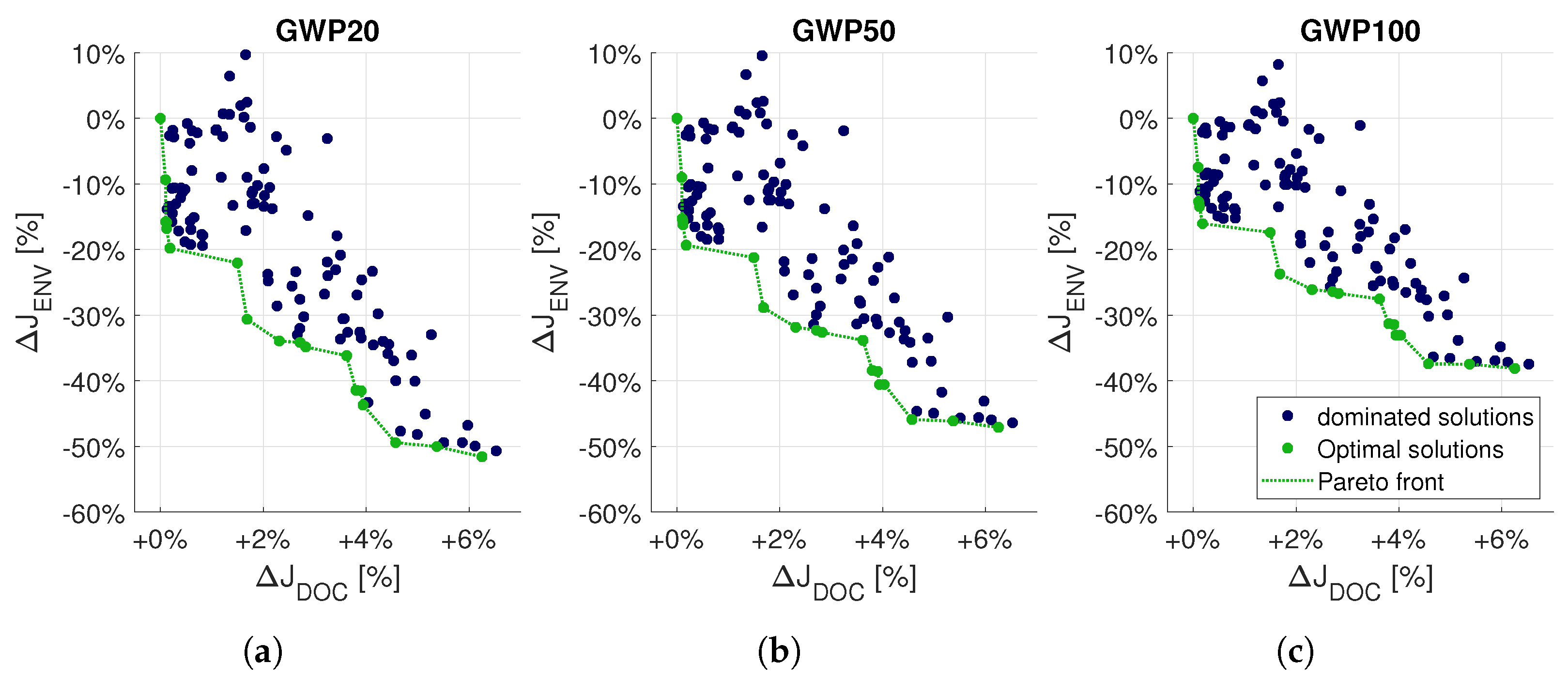
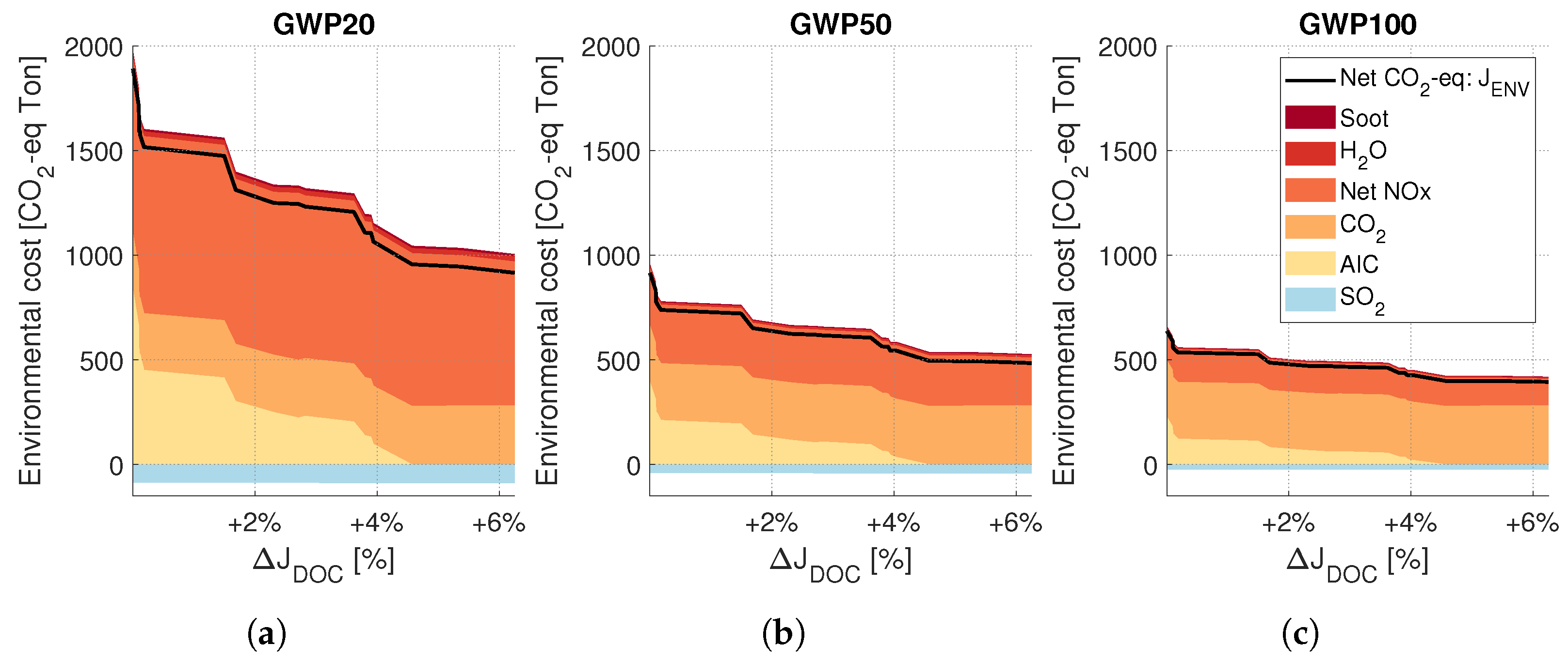
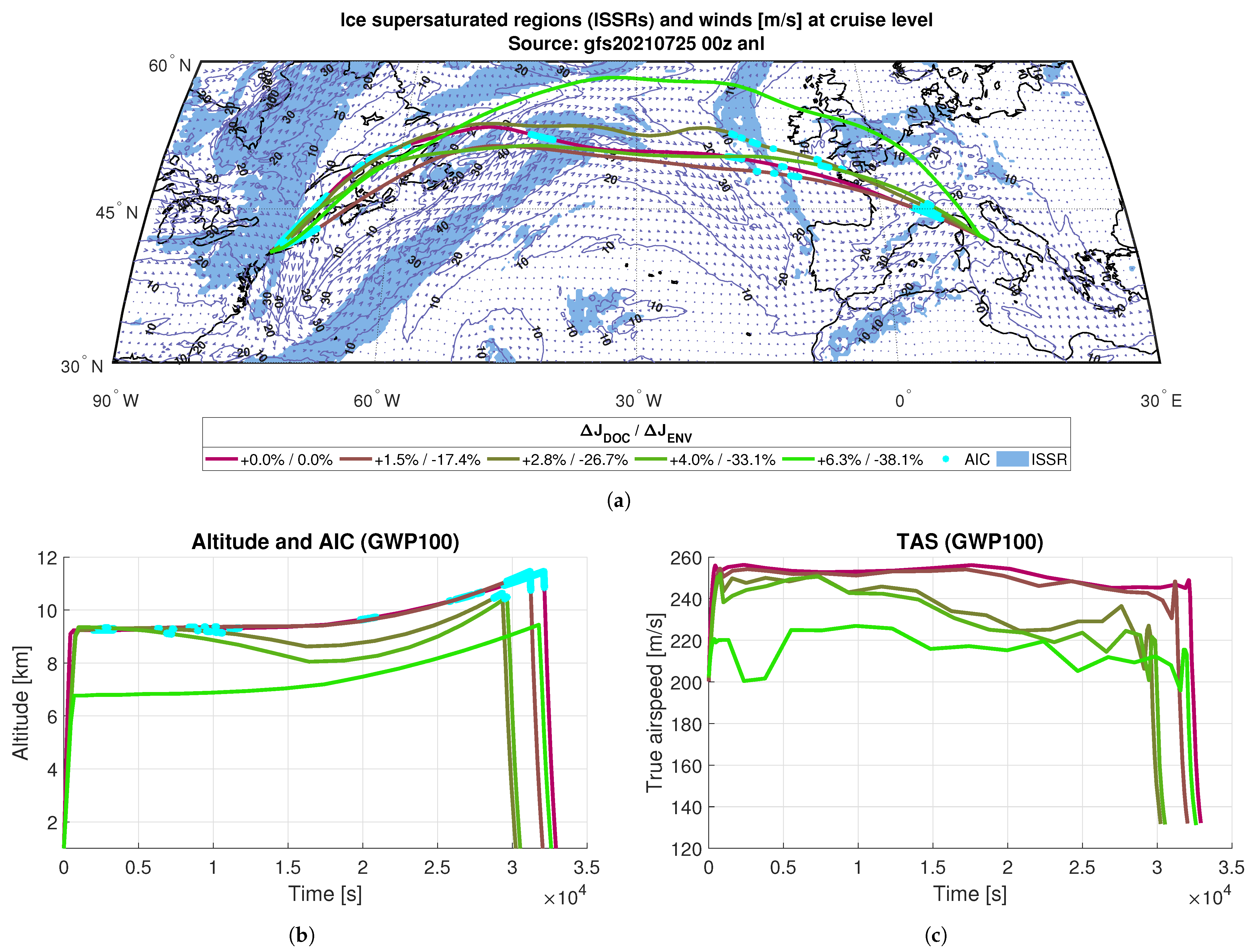
The initial and final waypoints of the descent phase are constrained to the TOD calculated in cruise optimization and to WP2. During all the idle descent, the fuel flow is at its minimum and can be considered constant, so the operating and environmental costs as defined in Equations (39) and (40) can be minimized only by reducing the descent time. TOD in cruise optimization is calculated for a maximum range idle descent, consequently the descent duration cannot be reduced without negatively impacting the descent range.

The states, controls, and final time of the descent phase are obtained by integrating the cruise states at TOD, along a cruise trajectory that lays on the geodesic directed towards WP2, assuming that at each step the true airspeed satisfies Equation (58).

3. Results

The results of the multi-objective and multi-phase trajectory optimization tool are presented for a test case involving a transatlantic commercial flight from Rome, Italy to New York, USA on a Boeing 747-100. The inputs of the test case optimization are reported in

Table 3. Inputs of the optimization tool for the test case flight from Rome to New York. WP1 and WP2 are respectively the start-of-climb and end-of-descent waypoints. Aircraft mass and time at WP2 are an output of the optimization.

	Lat	Lon	Altitude	Aircraft Mass	Date	Time (UTC)
WP1	41.9028	12.4964	1000 m	340 Ton	25 July 2021	00:00
WP2	40.7306	−73.9352	1000 m	-	-	-

. The number of nodes of the Chebyshev-Gauss-Lobatto (CGL) grid is user-defined. In this case, 20 nodes have been used for the cruise phase, while 10 nodes have been used for the climb and descent phases.

The output of the optimization tool is the Pareto set of optimal climb-cruise-descent trajectories from WP1 to WP2, where the objectives of the multi-objective optimization are the Direct Operating Cost (DOC), $J_{DOC}$, and the environmental cost, $J_{ENV}$, of the trajectory. For each trajectory on the Pareto front, it is not possible to further improve one of the two objective costs without degrading the other. The Pareto set of optimal solutions includes the DOC-optimal and the environmental-optimal trajectories that represent respectively the trajectories with the higher environmental and operating costs among the Pareto-optimal solutions. Each trajectory provided in output is represented as a time series of the states and controls of the aircraft to be processed by the Automatic Flight Control System (AFCS) of the aircraft for 4D trajectory tracking. In particular, the top-of-climb (TOC) and top-of-descent (TOD) waypoints are an output of the optimization, as well as the time of arrival at WP2.

Three multi-objective optimizations are performed considering an environmental cost function based on the Global Warming Potential (GWP) emission metric integrated for a 20-, 50-, and 100-year time horizons.

The plots in Figure 2 report the results of each optimization problem in the objective space. The axes of the objective spaces are expressed in terms of percentage variation with respect to the DOC-optimal trajectory, namely $\Delta J_{DOC}$ for the DOC and $\Delta J_{ENV}$ for the environmental cost. It must be noted that the DOC-optimal trajectory is the same for each of the three problems, since it is obtained optimizing with a cost function where the environmental term has a null weight. Figure 2 depicts the set of Pareto-optimal trajectories (in green) as well as the other sub-optimal feasible trajectories (in blue) produced by the optimization tool. Results show that by increasing the operating costs by 6.3% with respect to the DOC-optimal trajectory it is possible to reduce environmental costs by 51.6% for GWP₂₀, by 47.1% for GWP₅₀, and by 38.1% for the GWP₁₀₀ case. Nonetheless, in the flight planning phase the aircraft operator can choose the trajectory that better reflects its economic and environmental goals among the ones belonging to the Pareto set of optimal solutions, and submit it to the Air Traffic Controller (ATC).

Figure 3 illustrates a breakdown of the environmental cost of the Pareto-optimal set of solutions. The environmental cost is expressed in terms of CO₂-equivalent mass of emissions to underline the contribution of each climate forcing produced by the aircraft in the climb-cruise-descent arc. The first aspect that can be noticed is the reduction in the absolute value of the CO₂-equivalent emissions for increasing values of the GWP time horizon. This is because short-lived climate forcings such as aircraft-induced clouds (AIC) and NO_X have a smaller GWP in the long term when compared to the one of long-lived species such as CO₂. The other result apparent from Figure 3 is that the main strategy adopted by the optimization tool to mitigate the environmental cost of the trajectory is to reduce the formation of AIC along the path. In particular, it can be noticed that the environmental-optimal trajectory presents zero contrail formation.

Results from the GWP₁₀₀ case are now presented, to analyze the behavior of the optimization tool when shifting from DOC-optimal to environmental-optimal trajectory.

Figure 4a shows the lateral path of some of the solutions belonging to the Pareto set of optimal trajectories, including the DOC-optimal (purple) and the environmental-optimal path (green). The DOC-optimal solution ignores the presence of ice supersaturated regions (ISSRs) along the track, producing AIC on its trail, pursuing a flight track with low route extension (RE) and intercepting favorable tailwind conditions, especially in the north-western Atlantic region. On the other hand, the environment optimal trajectory adopts a greater route extension, as it can also be seen in

Table 4. The table reports trajectory data for the Pareto-optimal solutions for the environmental cost function based on GWP₁₀₀. The trajectories are numbered for increasing direct operating cost $J_{DOC}$ and decreasing environmental cost $J_{ENV}$, i.e., moving from left to right along the Pareto front in Figure 2c. The RE is calculated with respect to the great circle arc between WP1 and WP2 (6900 km), while AIC percentage length is expressed as a fraction of the track path distance. Boldface rows indicate the trajectories plotted in Figure 4.

	Op. Costs		Env. Costs (GWP100)		Route			Fuel	AIC
	JDOC	$\Delta$ JDOC	JENV	$\Delta$ JENV	Extension		Time	Mass	Length
ID	[k$]	[%]	[CO2-eq Ton]	[%]	[km]	[%]	[min]	[Ton]	[km]	[%]
1	77.11	-	637.4	-	218	+3.16%	549	85.6	1607	22.6%
2	77.18	+0.10%	589.9	−7.4%	91	+1.32%	524	85.6	1229	17.6%
3	77.19	+0.10%	556.6	−12.7%	150	+2.18%	476	85.7	1005	14.3%
4	77.20	+0.11%	555.4	−12.9%	85	+1.23%	517	85.7	966	13.8%
5	77.20	+0.12%	551.8	−13.4%	86	+1.24%	532	85.6	969	13.9%
6	77.25	+0.18%	535.2	−16.0%	97	+1.41%	515	85.8	850	12.1%
7	78.26	+1.50%	526.6	−17.4%	91	+1.32%	534	86.7	753	10.8%
8	78.41	+1.68%	486.3	−23.7%	187	+2.71%	501	86.5	575	8.1%
9	78.89	+2.31%	471.1	−26.1%	106	+1.53%	518	86.8	407	5.8%
10	79.20	+2.71%	469.1	−26.4%	117	+1.70%	495	87.3	367	5.2%
11	79.29	+2.82%	467.5	−26.7%	255	+3.69%	504	87.3	411	5.8%
12	79.90	+3.62%	461.9	−27.5%	77	+1.11%	518	87.9	363	5.2%
13	80.04	+3.80%	438.0	−31.3%	75	+1.09%	529	87.8	211	3.0%
14	80.12	+3.90%	437.1	−31.4%	372	+5.39%	507	87.9	220	3.0%
15	80.15	+3.94%	426.8	−33.0%	197	+2.86%	526	88.0	155	2.2%
16	80.22	+4.03%	426.7	−33.1%	170	+2.47%	509	88.1	123	1.7%
17	80.63	+4.57%	398.9	−37.4%	222	+3.22%	517	88.3	0	0.0%
18	81.25	+5.37%	398.7	−37.4%	427	+6.19%	539	88.9	0	0.0%
19	81.93	+6.25%	394.5	−38.1%	357	+5.17%	543	89.3	0	0.0%

, to avoid ISSRs and avoid AIC formation. Intermediate optimal solutions show a mixed behavior between the two limiting cases.

The altitude profile of the trajectories represented in Figure 4b shows how the DOC-optimal trajectory is characterized by a climbing cruise with a smoothly increasing flight path angle, pursuing a cruise altitude that maximizes the specific range (SPR) with respect to the DOC, regardless of AIC formation along the path. Increasing the weight of the environmental cost forces the optimization tool to reduce the altitude in the northern Atlantic area to avoid the ISSR visible in Figure 4a. This ISSR region is completely avoided by the environment optimal trajectory that deviates to the north along a longer route. The environment optimal trajectory also has a lower TOC altitude. This can be explained by the fact that lowering cruise altitude reduces NO_X emission, at a cost of increased CO₂ emissions. As it can be noticed from Figure 3, once AIC contribution to the CO₂-equivalent emissions is eliminated, a further reduction of the net CO₂-equivalent emissions can be obtained by a reduction of the net NO_X component, despise the increase of CO₂ emissions. The true airspeed (TAS) profile depicted in Figure 4c shows the tendency of a reduction of the TAS for increasing cruise altitudes, and fluctuations due to the variation of atmospheric conditions in the Global Forecast System (GFS) weather grid.

Figure 5 and Table 4 gather other trajectory data of the Pareto-optimal solutions for the GWP₁₀₀ case.

The route extension (RE) with respect to the great circle arc between WP1 and WP2 (6900 km) of the Pareto-optimal trajectories, represented in Figure 5a, shows a trend of increasing RE when moving towards environment optimal trajectories on the Pareto front. This is due to the fact that the optimization tool adopts longer routes to avoid ISSR and reduce AIC formation. The large scattering of the data is because the optimal lateral path is strictly dependent on lateral winds, so the DOC component of the cost function is not necessarily lower for small values of the RE.

Figure 5b,c show flight duration and fuel consumption of the optimal trajectories. Both tend to increase when leaning towards less cost efficient and greener trajectories, because the DOC cost function defined in Equation (39) is proportional to both flight time and fuel consumption, with scattering on fuel mass being lower due to the higher weight of fuel consumption on DOC with respect to flight operating cost per hour.

Figure 5d represents AIC length as a fraction of route length, and shows a complete elimination of consistent reduction in AIC formation when shifting from the DOC-optimal to the environmental-optimal solution. In particular, the length of along-track AIC is 1607 km for the DOC-optimal trajectory and is completely eliminated in the environmental-optimal trajectory.

4. Conclusions

This paper presents the development of a 4D trajectory optimization tool capable of generating a Pareto set of optimal trajectories in terms of Direct Operating Cost (DOC) and climate cost, based on the Global Warming Potential (GWP) emission metric, of the climb-cruise-descent arc of a commercial flight. The multi-phase and multi-objective optimization algorithm is based on a Chebyshev pseudospectral direct collocation method. The tool has been designed to be integrated within the Flight Management System (FMS) of a commercial aircraft, the Boeing 747-100, to perform 4D trajectory flight planning in a Free Route Airspace (FRA) context. The output of the trajectory optimization tool is a set of Pareto-optimal climb-cruise-descent trajectories ranging from the DOC-optimal to the climate-optimal trajectory, and it allows the aircraft operator to select the best compromise flight trajectory in the flight planning phase that satisfies both economic and environmental constraints.

The trajectory optimization tool has been employed on a test case flight from Rome to New York. Three separate multi-objective optimizations have been performed, using environmental cost functions based on the GWP integrated for a time horizon of 20, 50, and 100 years. For the GWP₁₀₀ case, the environmental-optimal trajectory grants a 38.1% reduction of the climate cost at the expense of a 6.3% increase of the DOC with respect to the DOC-optimal trajectory. In absolute terms, the environmental-optimal trajectory of the GWP₁₀₀ case reduces by 242.9 Ton the CO₂-equivalent emissions of the aircraft climate forcings at a cost of 4.8 k$ of DOC.

The environmental cost function takes into account the climate forcings of CO₂ and non-CO₂ emissions, as well as aircraft-induced clouds that are the main climate pollutant produced by aviation. In particular, the optimization algorithm showed good aircraft-induced clouds (AIC) formation avoidance capabilities, by adjusting the lateral and vertical trajectory path to avoid ice supersaturated regions (ISSR). In fact, the environmental-optimal trajectory for the test case based on GWP₁₀₀ managed to completely eliminate on-track AIC formation.

The accuracy of the trajectory optimization tool is affected by the reliability of weather data and forecasts, as well as by the uncertainties of the climate metrics that have been used for the estimation of the environmental cost index. However, the same tool developed in this paper can be used with more accurate weather data and climate metrics data as soon as they will be available to the scientific community. Future work will include the implementation of dynamic weather information and will take into account flight planning with adverse weather phenomena along the path, as well as the integration of the other flight phases occurring in terminal maneuvering areas in the proximity of airports that have a lower margin for climate impact mitigation but can be addressed for the reduction of noise pollution and the improvement of local air quality.

References

1. Lee, D.S.; Fahey, D.W.; Forster, P.M.; Newton, P.J.; Wit, R.C.; Lim, L.L.; Owen, B.; Sausen, R. Aviation and Global Climate Change in the 21st Century. Atmos. Environ. 2009, 43, 3520–3537. [Google Scholar] [CrossRef] [PubMed] [Green Version]
2. Eurocontrol, Free Route Airspace. Available online: https://www.eurocontrol.int/concept/free-route-airspace (accessed on 12 October 2021).
3. AIP Italia, ENAV, FRAIT—Free Route Italy. Available online: https://ec.europa.eu/transport/sites/default/files/AIC_A_2016_11.pdf (accessed on 12 October 2021).
4. EASA. European Aviation Environmental Report. 2019. Available online: https://www.easa.europa.eu/eaer/ (accessed on 12 October 2021).
5. Eurocontrol, Free Routes Airspace (FRA) Design Guidelines. Available online: https://www.eurocontrol.int/sites/default/files/2020-11/fra-design-guidelines-1.0.pdf (accessed on 12 October 2021).
6. Kistan, T.; Gardi, A.; Sabatini, R.; Ramasamy, S.; Batuwangala, E. An evolutionary outlook of air traffic flow management techniques. Prog. Aerosp. Sci. 2017, 88, 15–42. [Google Scholar] [CrossRef]
7. Betts, J.T. Survey of Numerical Methods for Trajectory Optimization. J. Guid. Control Dyn. 1998, 21, 193–207. [Google Scholar] [CrossRef]
8. Rao, A.V. Survey of Numerical Methods for Optimal Control. Adv. Astronaut. Sci. 2010, 135, 497–528. [Google Scholar]
9. Hagelauer, P.; Mora-Camino, F. Flight Management Systems and Aircraft 4D Trajectory Optimization. IFAC Proc. Vol. 1997, 30, 351–356. [Google Scholar] [CrossRef]
10. Bryson, A.; Ho, Y.C. Numerical solution of optimal programming and control problems. In Applied Optimal Control: Optimization, Estimation, and Control, 1st ed.; Taylor & Francis: Abingdon, UK, 1975; pp. 212–243. [Google Scholar]
11. Fornberg, B.; Sloan, D.M. A review of pseudospectral methods for solving partial differential equations. Acta Numer. 1994, 3, 203–267. [Google Scholar] [CrossRef]
12. The Optimal Control Problem. Practical Methods for Optimal Control and Estimation Using Nonlinear Programming, 2nd ed.; Society for Industrial and Applied Mathematics: Philadelphia, PA, USA, 2010; pp. 123–217. [Google Scholar]
13. Ross, I.M.; Fahroo, F. Pseudospectral Knotting Methods for Solving Nonsmooth Optimal Control Problems. J. Guid. Control. Dyn. 2004, 27, 397–405. [Google Scholar] [CrossRef]
14. Betts, J.T.; Cramer, E.J. Application of Direct Transcription to Commercial Aircraft Trajectory Optimization. J. Guid. Control Dyn. 1995, 18, 151–159. [Google Scholar] [CrossRef]
15. Soler, M.; Olivares, A.; Staffetti, E. Multiphase Optimal Control Framework for Commercial Aircraft Four-Dimensional Flight-Planning Problems. J. Aircr. 2015, 52, 274–286. [Google Scholar] [CrossRef]
16. Rao, A.V.; Benson, D.A.; Darby, C.; Patterson, M.A.; Francolin, C.; Sanders, I.; Huntington, G.T. Algorithm 902: GPOPS, A MATLAB Software for Solving Multiple-Phase Optimal Control Problems Using the Gauss Pseudospectral Method. ACM Trans. Math. Softw. 2010, 37, 1–39. [Google Scholar] [CrossRef]
17. Ross, I.M. Enhancements to the DIDO Optimal Control Toolbox. arXiv 2020, arXiv:math.OC/2004.13112. Available online: https://arxiv.org/pdf/2004.13112.pdf (accessed on 12 October 2021).
18. Rutquist, E.; Edvall, M.M. PROPT-Matlab Optimal Control Software. Available online: https://www.tomopt.com/docs/TOMLAB_PROPT.pdf (accessed on 12 October 2021).
19. Cassaro, M.; Gunetti, P.; Battipede, M.; Gili, P. Overview of the Multipurpose Aircraft Simulation Laboratory experience. In Proceedings of the 2013 Aviation Technology, Integration, and Operations Conference, Los Angeles, CA, USA, 12–14 August 2013. [Google Scholar]
20. Sirigu, G.; Battipede, M.; Gili, P.; Cassaro, M. FMS and AFCS Interface for 4D Trajectory Operations; SAE Technical Paper-2015; SAE International: Warrendale, PA, USA, 2015. [Google Scholar]
21. Mazzotta, D.G.; Sirigu, G.; Cassaro, M.; Battipede, M.; Gili, P. 4D Trajectory Optimization Satisfying Waypoint and No-Fly Zone Constraints. WSEAS Trans. Syst. Control 2017, 12, 221–231. [Google Scholar]
22. Nuic, A.; Poles, D.; Moulliet, V. BADA: An advanced aircraft performance model for present and future ATM systems. Int. J. Adapt. Control Signal Process. 2010, 24, 850–866. [Google Scholar] [CrossRef]
23. Hanke, C.; Nordwall, D. The simulation of a jumbo jet Transport aircraft Volume II: Modeling data. In D6-30643; The Boeing Company: Wichita, KS, USA, 1970. [Google Scholar]
24. Fahroo, F.; Ross, I.M. Direct Trajectory Optimization by a Chebyshev Pseudospectral Method. J. Guid. Control Dyn. 2002, 25, 160–166. [Google Scholar] [CrossRef] [Green Version]
25. Lufthansa Systems, Lido Flight 4D. Available online: https://www.lhsystems.com/solutions-services/operations-solutions/lidoflightplanning/lidoflight4D (accessed on 12 October 2021).
26. Montzka, S.A.; Dlugokencky, E.J.; Butler, J.H. Non-CO2 greenhouse gases and climate change. Nature 2011, 476, 43–50. [Google Scholar] [CrossRef]
27. Lee, D.; Fahey, D.; Skowron, A.; Allen, M.; Burkhardt, U.; Chen, Q.; Doherty, S.; Freeman, S.; Forster, P.; Fuglestvedt, J.; et al. The contribution of global aviation to anthropogenic climate forcing for 2000 to 2018. Atmos. Environ. 2021, 244, 117834. [Google Scholar] [CrossRef] [PubMed]
28. ICAO. Assessing Current Scientific Knowledge, Uncertainties and Gaps in Quantifying Climate Change, Noise and Air Quality Aviation Impacts. Available online: https://www.icao.int/environmental-protection/Documents/CaepImpactReport.pdf (accessed on 12 October 2021).
29. Park, S.G.; Clarke, J.P. Vertical Trajectory Optimization to Minimize Environmental Impact in the Presence of Wind. J. Aircr. 2016, 53, 725–737. [Google Scholar] [CrossRef] [Green Version]
30. Sirigu, G.; Clarke, J.P.; Battipede, M.; Gili, P. Hybrid Particle Swarm Optimization with Parameter Fixing: Application to Automatic Taxi Management. J. Air Transp. 2020, 28, 36–48. [Google Scholar] [CrossRef]
31. Kärcher, B. Formation and radiative forcing of contrail cirrus. Nat. Commun. 2018, 9, 117834. [Google Scholar] [CrossRef] [PubMed]
32. Sridhar, B.; Ng, H.K.; Chen, N.Y. Aircraft Trajectory Optimization and Contrails Avoidance in the Presence of Winds. J. Guid. Control Dyn. 2011, 34, 1577–1584. [Google Scholar] [CrossRef]
33. Soler, M.; Zou, B.; Hansen, M. Contrail Sensitive 4D Trajectory Planning with Flight Level Allocation Using Multiphase Mixed-Integer Optimal Control. In Proceedings of the AIAA Guidance, Navigation, and Control (GNC) Conference, Boston, MA, USA, 19–22 August 2013. [Google Scholar]
34. Irvine, E.A.; Hoskins, B.J.; Shine, K.P. A simple framework for assessing the trade-off between the climate impact of aviation carbon dioxide emissions and contrails for a single flight. Environ. Res. Lett. 2014, 9, 064021. [Google Scholar] [CrossRef]
35. Rosenow, J.; Fricke, H. Individual Condensation Trails in Aircraft Trajectory Optimization. Sustainability 2019, 11, 6082. [Google Scholar] [CrossRef] [Green Version]
36. Teoh, R.; Schumann, U.; Majumdar, A.; Stettler, M.E.J. Mitigating the Climate Forcing of Aircraft Contrails by Small-Scale Diversions and Technology Adoption. Environ. Sci. Technol. 2020, 54, 2941–2950. [Google Scholar] [CrossRef] [PubMed]
37. Matthes, S.; Lührs, B.; Dahlmann, K.; Grewe, V.; Linke, F.; Yin, F.; Klingaman, E.; Shine, K.P. Climate-Optimized Trajectories and Robust Mitigation Potential: Flying ATM4E. Aerospace 2020, 7, 156. [Google Scholar] [CrossRef]
38. Myhre, G.; Shindell, D.; Pongratz, J. Intergovernmental Panel on Climate Change, Anthropogenic and Natural Radiative Forcing. In Climate Change 2013–The Physical Science Basis: Working Group I Contribution to the Fifth Assessment Report of the Intergovernmental Panel on Climate Change; Cambridge University Press: Cambridge, UK, 2014; pp. 659–740. [Google Scholar]
39. DuBois, D.; Paynter, G.C. Fuel Flow Method2 for Estimating Aircraft Emissions. In Non-Conference Specific Technical Papers-2006; SAE International: Warrendale, PA, USA, 2006. [Google Scholar]
40. European Union Aviation Safety Agency. ICAO Aircraft Engine Emissions Databank. Available online: https://www.easa.europa.eu/domains/environment/icao-aircraft-engine-emissions-databank (accessed on 12 October 2021).
41. Schumann, U. A contrail cirrus prediction model. Geosci. Model Dev. 2012, 5, 543–580. [Google Scholar] [CrossRef] [Green Version]
42. Kim, I.; de Weck, O. Adaptive weighted-sum method for bi-objective optimization: Pareto front generation. Struct. Multidiscipl. Optim. 2005, 29, 149–158. [Google Scholar] [CrossRef]
43. Trefethen, L.N. Equispaced Points, Runge Phenomenon. In Approximation Theory and Approximation Practice, Extended Edition; Society for Industrial and Applied Mathematics: Philadelphia, PA, USA, 2019; pp. 95–102. [Google Scholar]
44. Trefethen, L.N. Chebyshev Differentiation Matrices. In Spectral Methods in MATLAB; Society for Industrial and Applied Mathematics: Philadelphia, PA, USA, 2000; pp. 51–59. [Google Scholar]
45. Waldvogel, J. Fast Construction of the Fejér and Clenshaw–Curtis Quadrature Rules. BIT Numer. Math. 2006, 46, 195–202. [Google Scholar] [CrossRef] [Green Version]
46. National Weather Service: Pressure Altitude. Available online: https://www.weather.gov/media/epz/wxcalc/pressureAltitude.pdf (accessed on 12 October 2021).
47. Picard, A.; Davis, R.S.; Gläser, M.; Fujii, K. Revised formula for the density of moist air (CIPM-2007). Metrologia 2008, 45, 149–155. [Google Scholar] [CrossRef]
48. World Meteorological Organization (WMO). Cloud Atlas. Available online: https://cloudatlas.wmo.int/aircraft-condensation-trails.html (accessed on 12 October 2021).
49. Sonntag, D. Advancements in the field of hygrometry. Meteorol. Z. 1994, 3, 51–66. [Google Scholar] [CrossRef]
50. Federal Aviation Administration, Benefit-Cost Analysis: Aircraft Operating Costs. Available online: https://www.faa.gov/regulations_policies/policy_guidance/benefit_cost/media/econ-value-section-4-op-costs.pdf (accessed on 12 October 2021).
51. Federal Aviation Administration, Benefit-Cost Analysis: Economic Values Related to Aircraft Performance. Available online: https://www.faa.gov/regulations_policies/policy_guidance/benefit_cost/media/econ-value-section-6-perf-factors.pdf (accessed on 12 October 2021).
52. Schumann, U.; Penner, J.E.; Chen, Y.; Zhou, C.; Graf, K. Dehydration effects from contrails in a coupled contrail—Climate model. Atmos. Chem. Phys. 2015, 15, 11179–11199. [Google Scholar] [CrossRef] [Green Version]
53. Yang, X.S. Chapter 14—Multi-Objective Optimization. In Nature-Inspired Optimization Algorithms; Yang, X.S., Ed.; Elsevier: Oxford, UK, 2014; pp. 197–211. [Google Scholar]
54. Bellman, R.E. The Structure of Dynamic Programming Process. In Dynamic Programming; Princeton University Press: Princeton, NJ, USA, 1957; pp. 81–115. [Google Scholar]
Figure 1. Scheme of the averaging method used to pass along-trajectory weather information to the CGL nodes p of the optimization algorithms. The number of sub-CGL nodes s is chosen to have a spatial resolution similar to the GFS grid with weather data. The gradient color map represents different values of a generic GFS data variable.
Aerospace 08 00395 g001
Figure 2. Pareto-optimal (green) and dominated sub-optimal solutions (blue) of the three multi-objective optimization problems, with environmental cost function based on: (a) GWP20, (b) GWP50, (c) GWP100.
Aerospace 08 00395 g002
Figure 3. Individual climate forcing components of the environmental cost J E N V , expressed in CO2-equivalent Ton, for environmental cost function based on: (a) GWP20, (b) GWP50, (c) GWP100. Negative values for SO2 indicate a cooling forcing.
Aerospace 08 00395 g003
Figure 4. Some of the Pareto-optimal trajectories for the GWP100 case, ranging from the optimal DOC trajectory (purple) to the climate-optimal trajectory (light green): (a) lateral path plotted on a map, with cyan segments indicating along track AIC formation, blue areas representing ISSR, and wind speeds expressed by a contour and vector map; (b) altitude profile plotted against time with along track AIC formation; (c) TAS profile. The atmospheric conditions represented in (a) are evaluated at an indicative cruise level, given by the average altitude of each plotted trajectory as a function of the longitude.
Aerospace 08 00395 g004
Figure 5. The plots show trajectory data of the Pareto-optimal solutions for the environmental cost function based on GWP100: (a) route extension with respect to the great circle distance between WP1 and WP2; (b) flight duration; (c) fuel consumption; (d) fraction of AIC length with respect to route length, plotted against Δ J D O C . Green dots represent trajectories plotted in Figure 4.
Aerospace 08 00395 g005