Article

Comparative Study of Different Algorithms for a Flight Control System Design and the Potentiality of Their Integration with a Sidestick

Department of Flight Dynamics and Control, Moscow Aviation Institute, 125993 Moscow, Russia
*
Author to whom correspondence should be addressed.
Aerospace 2021, 8(10), 290; https://doi.org/10.3390/aerospace8100290
Submission received: 26 August 2021 / Revised: 1 October 2021 / Accepted: 3 October 2021 / Published: 7 October 2021
(This article belongs to the Special Issue Aerospace Guidance, Navigation and Control)

Abstract

:
The modern trend of developing highly automated aircraft is characterized by a transition from traditional methods and technical solutions to innovative approaches in order to control the system, inceptor and display design. This paper deals with the development and comparison of flight control system algorithms based on inverse dynamics, H-infinity and traditional feedback methods. The integration of a controller based on inverse dynamics with a novel type of sidestick, shaping the pilot output signal such that it is proportional to the control force (force sensing control—FSC), is studied. The inverse dynamics-based controller is chosen, as it provides a variance of error that is up to 2.3 times less than that of the feedback gains and up to 1.5 times less than that of the H-infinity controller in a pitch tracking task. The synergetic effect arising from the proposed integration is also evaluated. The evaluation of the effectiveness of the methods is carried out through mathematical modeling of the pilot–aircraft system and ground-based simulations on a helicopter mathematical model in a pitch tracking task.

1. Introduction

Modern computation capabilities and the widespread use of high augmentation in the flight control systems of aerospace vehicles have been accompanied by research of new approaches to control algorithm design, making use of the available technology. The inverse dynamics technique is one of those control algorithms developed in recent years that make it possible to considerably change the dynamics of an aircraft, making the control problem easier to solve.
Over the years, this technique has been used in a variety of applications both in fixed-wing aircraft [1,2] and in rotorcraft [3,4].
Robustness is one of the requirements in flight control system designs. Inverse dynamics is very demanding toward this requirement, as they are sensitive to changes in the mathematical models of the controlled element or of the processes affecting the controlled element, such as winds and disturbances. When these uncertainties are present, the inverse dynamics-based controller used in the feedforward loop cannot correct for tracking errors [5]. In [6,7], the author established the boundaries of controlled element uncertainties that would be acceptable when using inverse dynamics. Inverse dynamics would be effective only if the size of the uncertainties in the nominal plant is smaller than the size of the nominal plant divided by its condition number. Here, the size of the plant and the size of the uncertainties are both measured as the 2-norm of their transfer functions. Moreover, the condition number of the plant is the product of the size of the plant and the size of its inverse. The method developed in [6] allows the use of inverse dynamics only when these boundaries are observed. This makes the technique applicable only to a limited number of control problems.
Inverse dynamics in general can be applied to both linear and nonlinear control problems. As a nonlinear control technique, inverse dynamics is used to make an appropriate coordinate transformation of a nonlinear controlled element [8] so that any linear control technique can be applied to the resulting linear controlled element. This is illustrated in [5] and [9], where nonlinear dynamics inversion is used in the inner loop and a PID-type controller is used in the outer loop to achieve both reference tracking and robustness against modeling uncertainties and disturbances. The same two-loop approach is used in [10], where the inner loop uses the inverse dynamics technique to linearize the nonlinear plant, and the outer loop uses an H∞-based controller to provide robustness. Flight controllers based on inverse dynamics principles can also be designed using machine learning principles as in [11], where inverse dynamics is approximated using a nonlinear regression neural network and used in the same fashion as feedback linearization to allow the application of a PI controller.
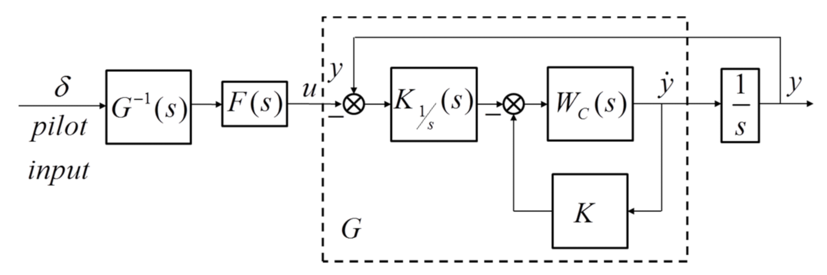
As a linear control technique, the inverse dynamics method has mostly been used in the feedforward control loop to support feedback controllers. In this form, its integration with reference model techniques has been studied in [12]. Here, the desired dynamics of the whole system, that is, the controlled element plus the control system, are computed via the use of reference models. The desired computed dynamics are then applied to the inverse dynamics in order to calculate the actuator positions needed to achieve the required performance.
This method, however, still requires an exact model of the controlled aircraft. Therefore, a PID-type compensator must be added in order to provide robustness against modeling uncertainties and disturbances as in [3].
Inverse dynamics as a linear control method has also been used in [13] to decouple the dynamics of the controlled element and achieve good tracking performance, and robustness is provided by a reference model and its inverse. This method, however, uses several loops in the control algorithm, making it difficult and expensive to implement.
In [14], a detailed account of the linear inverse dynamics approach for the improvement of helicopter flying qualities is given, and robustness is achieved using a PI controller.
Another popular approach to the design of flight control systems is the H-infinity method, which appeared in the seminal works of Zames [15]. This approach takes advantage of singular values to synthesize an optimal controller that minimizes a cost function representing robustness and performance of the system. The H-infinity method has been used extensively for flight control as in [16], where linear H-infinity-based controllers are used with a gain scheduling method extended for dynamical systems in order to take advantage of the robustness of H-infinity in nonlinear control.
The H-infinity technique has also been applied to all sorts of rotorcraft control problems. In [17], the technique is applied to a two-degree-of-freedom helicopter using a sensitivity minimization approach, which consists in minimizing the sensitivity of the system to external disturbances, which can also be additive uncertainties. In [18], the same sensitivity minimization approach of the H-infinity implementation is used to robustly stabilize a helicopter with a suspended load. One of the problems with this approach, however, is that there is no systematic way of choosing the weight matrices that generalize to all control problems.
Another approach used to apply the H-infinity optimization is loop shaping [19,20,21]. The basic idea of this technique is to specify the design requirements in terms of singular values of the open-loop system. Weight matrices are then used to achieve the open-loop requirements before applying the H-infinity optimization procedure to find a controller that satisfies the said requirements.
Inverse dynamics and H-infinity techniques have been used together in [22,23]. In both of these cases, they are used in different control loops where inverse dynamics eliminates the need for gain scheduling, and the H-infinity controller designed with additional shaping filters provides reference tracking and robustness.
This paper presents a linear approach where the inverse dynamics technique is used with a PI controller to provide good tracking performances and robustness to uncertainties and disturbances. A second approach is presented, where the H-infinity optimization technique is used in its loop-shaping implementation along with an inverse dynamics-based filter to form a controller that inherits the performance of the inverse dynamics technique and the robustness of the H-infinity technique.
Additionally, a comparative analysis was carried out assessing the effectiveness of the traditional feedback gains controller, the inverse dynamics controller and the H-infinity-based controller. The analysis was conducted via mathematical modeling of the pilot–aircraft system to study the integration of the human pilot in the control loop and via ground-based simulations to study the feasibility of the proposed control algorithms and the impact of a real human pilot.
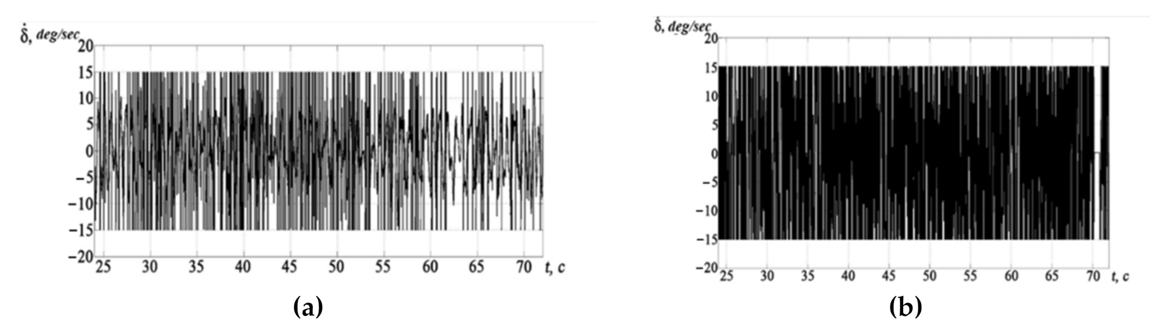
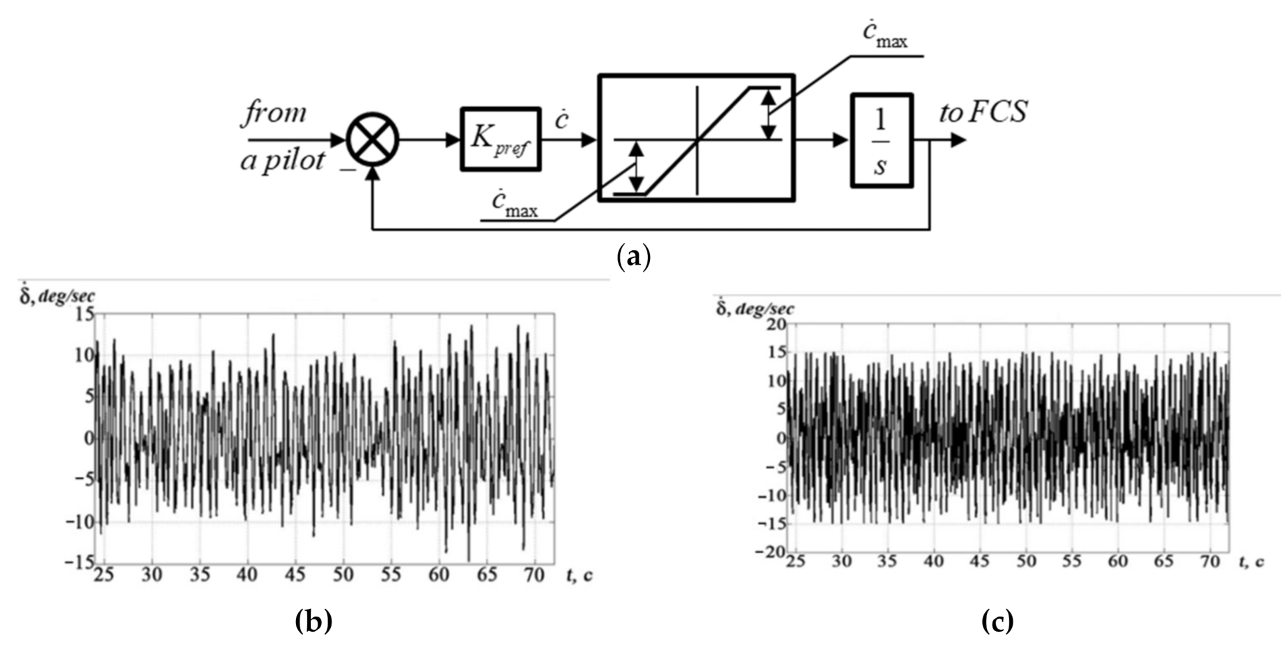
This analysis revealed the issue of high actuator rate demands that arises when using inverse dynamics. This issue can lead to certain undesirable effects, such as pilot-induced oscillations (PIO). This paper presents a nonlinear prefilter used as a solution to this problem in order to insure a safe operation of the actuators and the safety of the entire system.
Besides the analysis introduced above, an additional investigative study was carried out with different inceptors and types of pilot output signals with the goal of defining the best way of their integration with the proposed techniques.

2. Inverse Dynamics Design Procedure

2.1. Inverse Dynamics Potentialitites

The control algorithms designed following the inverse dynamics method as developed in [13] are as shown in Figure 1, where Wc(s) is a linearized model of the flying vehicle that is being controlled.
Inverse dynamics is used in the feedforward loop to improve tracking performance and, as such, requires a stable system [24]. Stability is therefore provided by a set of feedback gains K, and the element K 1 / s s = K s Ts + 1 s provides robustness to the system [14]. The controlled element with stabilizing gains and the robustness element form the system G, which is then used with inverse dynamics.
In Figure 1, δ is the vector of signals from the pilot’s inceptors. In the case of a helicopter, these signals come from the longitudinal and lateral cyclic stick, collective stick and pedals; G 1 s is the inverse dynamics and   y ˙ is the vector of angular rates (pitch rate, roll rate and yaw rate) and climb rate (q, p, r and w, respectively).
The proposed algorithms bring the frequency response   y ˙   ( j ω ) δ ( j ω ) closer to the gain response in a wide frequency range and decouple the control axes, which is the main motivation for using inverse dynamics as given in [13].
When the controlled element dynamics are y ( j ω ) δ ( j ω ) , the frequency response is then close to the integral element.
In Figure 1, the element F(s), as shown in [14], equalizes the order of the numerator and that of the denominator, therefore making the system feasible.
The frequency response of the system presented in Figure 1 can be seen in Figure 2, showing the characteristics described above. As it can be seen, for the pitch channel, the inverse dynamics brings the controlled element close to the integral element in almost the entire frequency range. This is seen in contrast to the characteristics provided by the feedback gains only.

2.2. Inverse Dynamics Computation

The inverse dynamics is computed analytically, following the technique given in [24]. This technique starts with a dynamical system given in state space form. The system G used in this paper contains nonlinear elements, such as time delays and nonlinear actuators. Therefore, it needs to be linearized and represented in state space form before calculating the inverse dynamics. This is conducted using the Jacobian linearization method given in [25], resulting in matrices A, B, C and D.
Using the matrices obtained above, the state space representation can be constructed as shown by Equations (1) and (2).
sX(s) = AX(s) + BU(s)
  Y ˙   ( s ) = C X ( s ) + D U ( s )
where X is the state vector, U is the input vector, D is the feedforward matrix, and C is the matrix relating the state vector X to the output vector Y of the system G.
The transfer function representation can then be derived by re-writing (1) in terms of X(s) as shown in Equation (3) and substituting it in (2) to obtain Equation (4), with the feedforward matrix D being a zero matrix:
X(s) = (sI − A)−1 BU(s)
  Y ˙   ( s ) = C ( sI A ) 1 B U ( s )
The relationship between the state space representation and the matrix of transfer functions can then be written as
  Y ˙   ( s ) U ( s ) = C ( sI A ) 1 B
Equation (5) results in a matrix of transfer functions, where each element gij connects the input i to the output j. Each of these transfer functions is then inverted individually such that for a transfer function g ij = y j ˙ u i , the inverse dynamics is given by g i j = u i y ˙ j .

3. H-Infinity Design Procedure

The H∞ technique, in all its formulations, is a frequency domain design technique.
The approach presented in this paper is based on the shaping of the open loop such that the closed-loop system will allow good reference tracking at low frequencies and disturbance rejection at high frequencies.

3.1. H∞ Optimization

The objective is to compute a stable feedback controller H(s) that stabilizes the vehicle and maintains good performance even in the presence of uncertainties.
This goal can be expressed in the H∞ optimization framework such that the problem becomes that of finding a controller H(s) satisfying the condition given in Equation (6). This is a stability condition for feedback systems as given in [26].
H I I G s H 1 M 1 1 ϵ max φ min  
where, H is the H∞ controller, I is an identity matrix, Gs is the shaped plant as seen in Section 3.2, and M is one of the elements resulting from the left factorization of Gs [27]. It can be computed in a simplified manner using the solution to the Riccati equations as shown below, and ϵmax is the maximum stability margin calculated as
ϵ max 1 = φ min = 1 + λ max ( XZ ) 1 / 2  
where, λmax finds the maximum eigenvalues, and X and Z are the solutions to the generalized algebraic Riccati equations shown in Equation (8).
( A BS 1 D T C ) T X + X ( A BS 1 D T C ) XBS 1 B T X + C T ( I DS 1 D T ) C = 0 ( A BD T R 1 C ) Z + Z ( A BD T R 1 C ) T ZC T R 1 CZ + B ( I D T R 1 D ) B T = 0
where,
S = I + D T D R = I + DD T
and
M = R 1 / 2 + R 1 / 2 C ( sI A IC ) 1 E
E = ZC T + BD T R 1
A, B, C and D are the state space matrices of the shaped system Gs, which is the mathematical model of the vehicle augmented with predefined filters as shown in the next subsection.

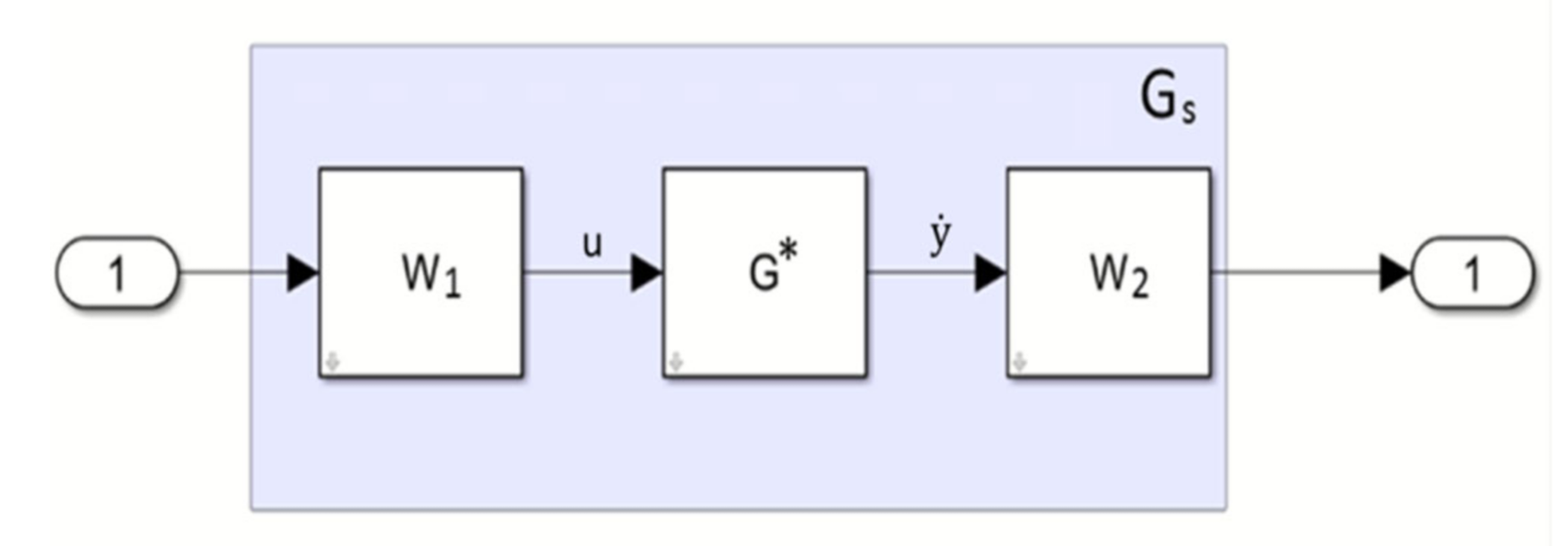
3.2. Shaped System Gs(s)

The system Gs (s) is formed by adding two shaping filters, W1 (s) and W2 (s), as shown in Equation (12) and in Figure 3.
G s s = W 2 s G s W 1 s
where G s is the vehicle model with stabilizing gains, which is equivalent to G(s) without the K 1 / s s = K s Ts + 1 s element.
The problem now is to find or compute the shaping filters such that W1(s) provides good tracking performance and W2(s) provides disturbance attenuation.
Disturbances are almost always in the higher frequency range. Therefore, W2 is chosen to be a first-order low-pass filter of the form
W 2 = K 1 Ts + 1
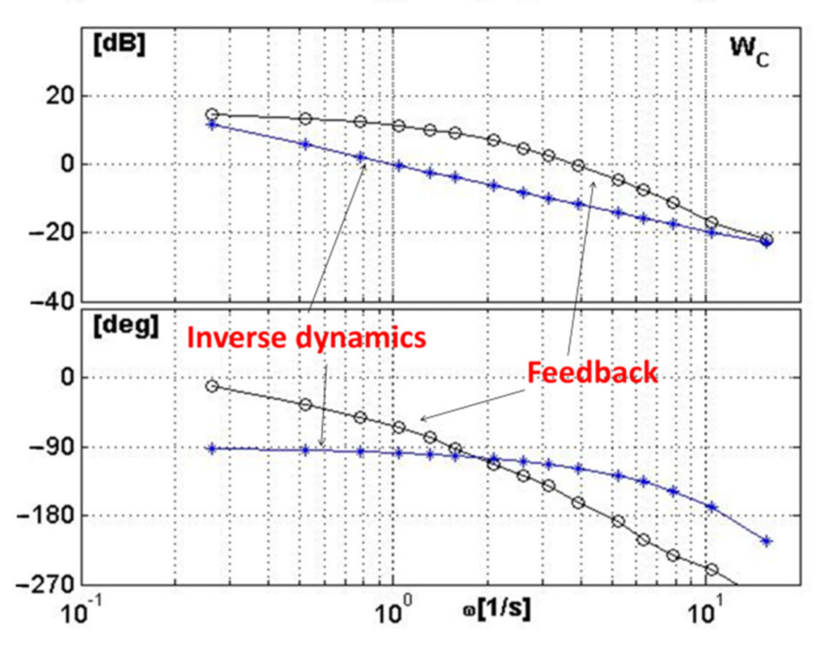
As discussed previously with inverse dynamics, we need the frequency response of   y ˙   ( j ω ) δ ( j ω ) to be equivalent to the gain response.
The frequency response of the shaped system G s should then be close to the integral K 3 s , which will result in a closed loop whose response is equivalent to a gain in the low frequency range.
The choice of W1 can then be motivated as follows:
G s = K 3 s   if   and   only   if   G W 1 = K 3 s W 1 = K 3 s G   1
where G   1 is the inverse dynamics of G . It is also worth noting that Equation (14) is valid only in the frequency range lower than the cutoff frequency of W2.
The peculiarity that can be seen here is that the inverse dynamics becomes included in the H-infinity controller. This integration was not explicit. It was, rather, an emergent feature of the frequency response requirement, and it allows the H-infinity controller to decouple the control axes of the vehicle and to provide good tracking performance while the H-infinity controller itself has the robustness features.

3.3. Dynamic Controller H(s)

After shaping the mathematical model of the vehicle, the matrices A, B, C and D of the shaped system and the solutions to the Riccati equations are used to compute the controller H(s) in state space form as shown in Equation (15).
H s = A + B W + φ 2 ( L T ) 1 Z C T C + D W                                   φ 2 ( L T ) 1 Z C T B T X D T
where
L = 1 φ 2 I + X Z W = S 1 D T C + B T X
The optimal overall stability margin φ is calculated as given in Equation (7). The value of this margin may differ from the classical SISO stability margins, as it is calculated using the eigenvalues of the coupled MIMO system. If the maximum eigenvalues are complex numbers, this results in a complex φ , which in turn will introduce a singularity as it is used to calculate the controller H(s). When this happens, it is necessary to modify the parameters of the shaped system used such that the maximum eigenvalues are not complex. This process is conducted iteratively, with some engineering intuition, as there is no formal way to tune the system.
It is also worth noting that Equation (16) uses φ and not φ min, because a controller can be computed for any value of φ >   φ min. However, we have to keep in mind that φ is inversely proportional to the stability margin and, therefore, with an increase in its value, the stability margin consequently decreases, and from the basics of control theory, it follows that tracking performance increases. Therefore, there is a fundamental tradeoff between the stability margin and performance, and this can be tuned by changing the value of φ used.

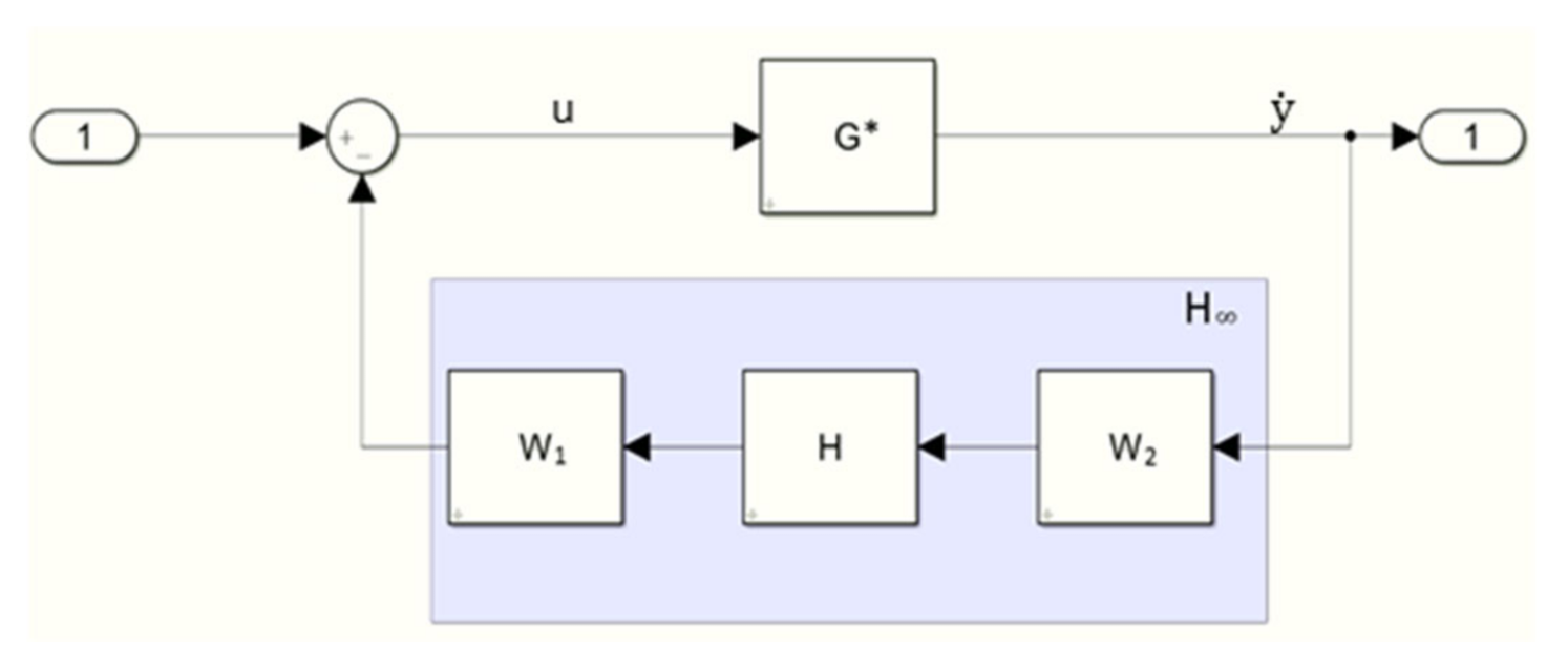
3.4. H∞ Controller Implementation

The previous section computed the controller H(s) that will provide robust stability to the system. The final feedback controller is obtained as the product of H(s) and the shaping filters as shown in Figure 4.
H = W 1 H W 2

3.5. H∞ Design Summary

The design of the H∞ controller can be summarized as follows:
1.
Find the stabilizing gains for the nominal system via classical methods or pole placement and obtain the system G;
2.
Compute the inverse dynamics G   1 ;
3.
Define the shaping filter W1 using inverse dynamics for reference tracking and W2 using a low-pass filter for high-frequency noise or disturbance rejection and build the shaped system Gs;
4.
Calculate the controller H:
  • Solve the algebraic Riccati equations of the shaped system Gs;
  • Calculate the optimal ϵmax and φ min using the solutions to the Riccati equations;
  • Compute the controller H;
  • Construct the final dynamic feedback controller such that H∞(s) = W1(s) H(s) W2(s).

4. Research Plan

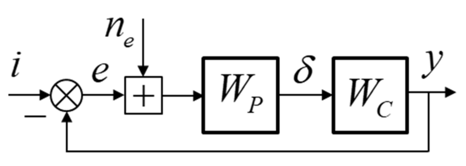
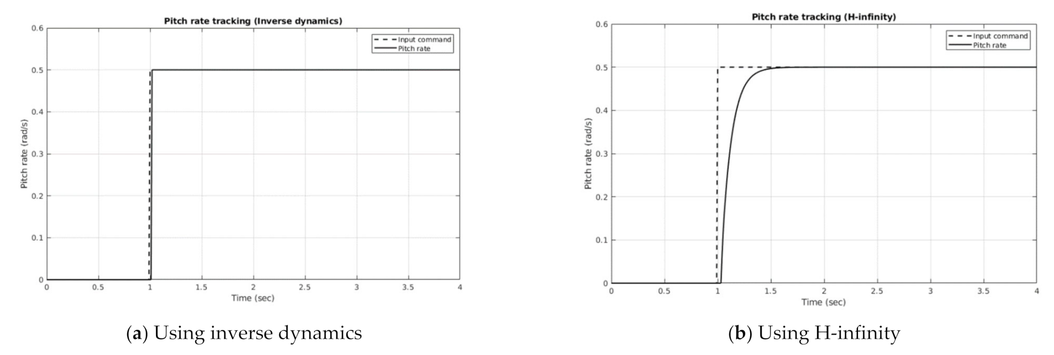
The controllers designed above were evaluated for a pitch angle tracking task with the dynamical model of a helicopter. Here, pilot actions can be represented as a single-loop compensatory system as shown in Figure 5. Another point to note is that the pilot signals δ (from the longitudinal cyclic) can be either proportional to the inceptor displacement (deflection) or proportional to the force applied on the inceptor.
The effectiveness of the proposed algorithms was studied using ground-based simulation and mathematical modeling of the pilot–aircraft system.

4.1. Mathematical Modeling of the Pilot–Aircraft System

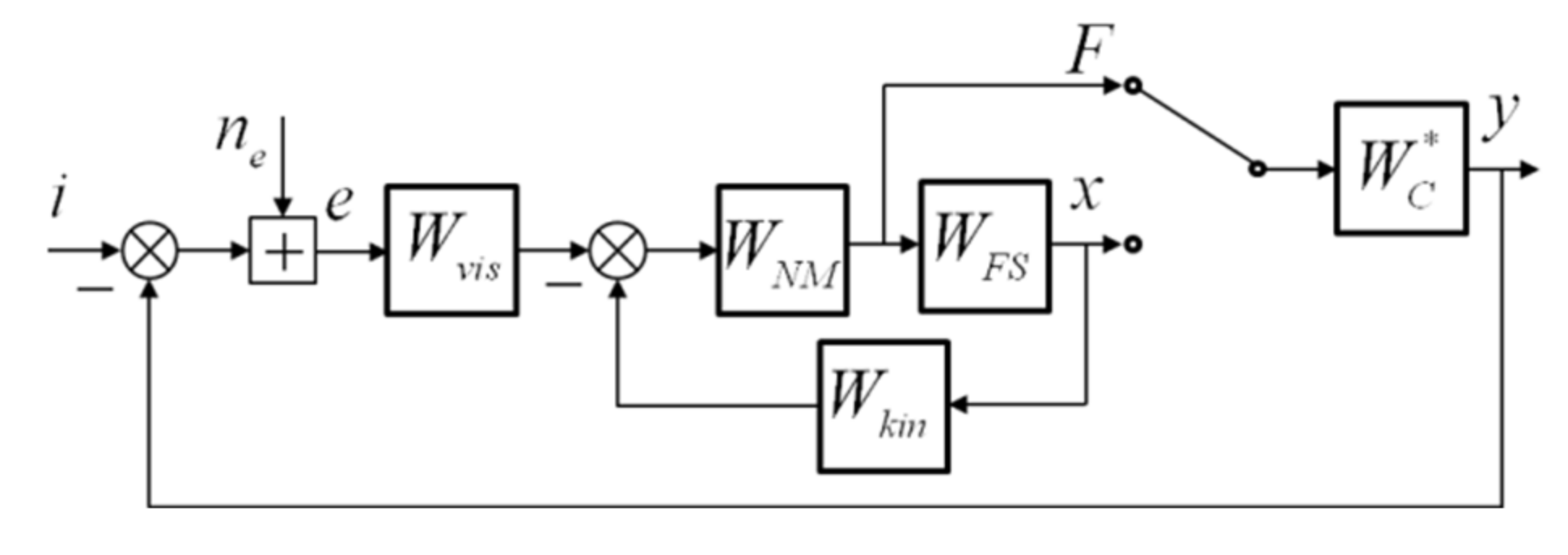
Mathematical modeling was carried out using a modified structural model of the pilot developed in [28] and shown in Figure 6.
where i is the input signal, e is the error signal, x is the stick deflection (displacement), F is the force applied on the stick by the pilot, y is the output of the pilot vehicle system, and Wc is the controlled element dynamics;
  • W vis = K L T L   j ω T I   j ω e τ   j ω is the model of visual information perception and compensation; W kin = K n ( j ω ) 2 T n 2 ( j ω ) 2 + 2 T n j ω + 1 is the model of proprioceptive information perception and compensation;
  • W NM = 1 ( T N j ω + 1 )   1 ( T N 2 j ω 2 + 2 ζ N   j ω + 1 ) is the neuromuscular system model;
  • W FS = K FS j ω 2 + 2 ζ FS ω FS   j ω + ω FS 2 ) is the inceptor model; and
  • ne is the pilot noise (remnant) characterized by the spectral density S n e n e = K n e π σ e 2 + T L 2 σ   e ˙ 2 1 + T L 2 ω 2 , where σ e 2 and σ   e ˙ 2 are the variance of error and its derivative, respectively; K n e = 0 . 01 ; and Wc is the controlled element, which is the mathematical model of the vehicle and the control system. The parameter vector of the structural model a = (TL, KL, TN, KN) is calculated by running the minimization criterion I = min ( σ e 2 ), where the variance of error σ e 2 is determined as given in [29].
The structural model shown in 
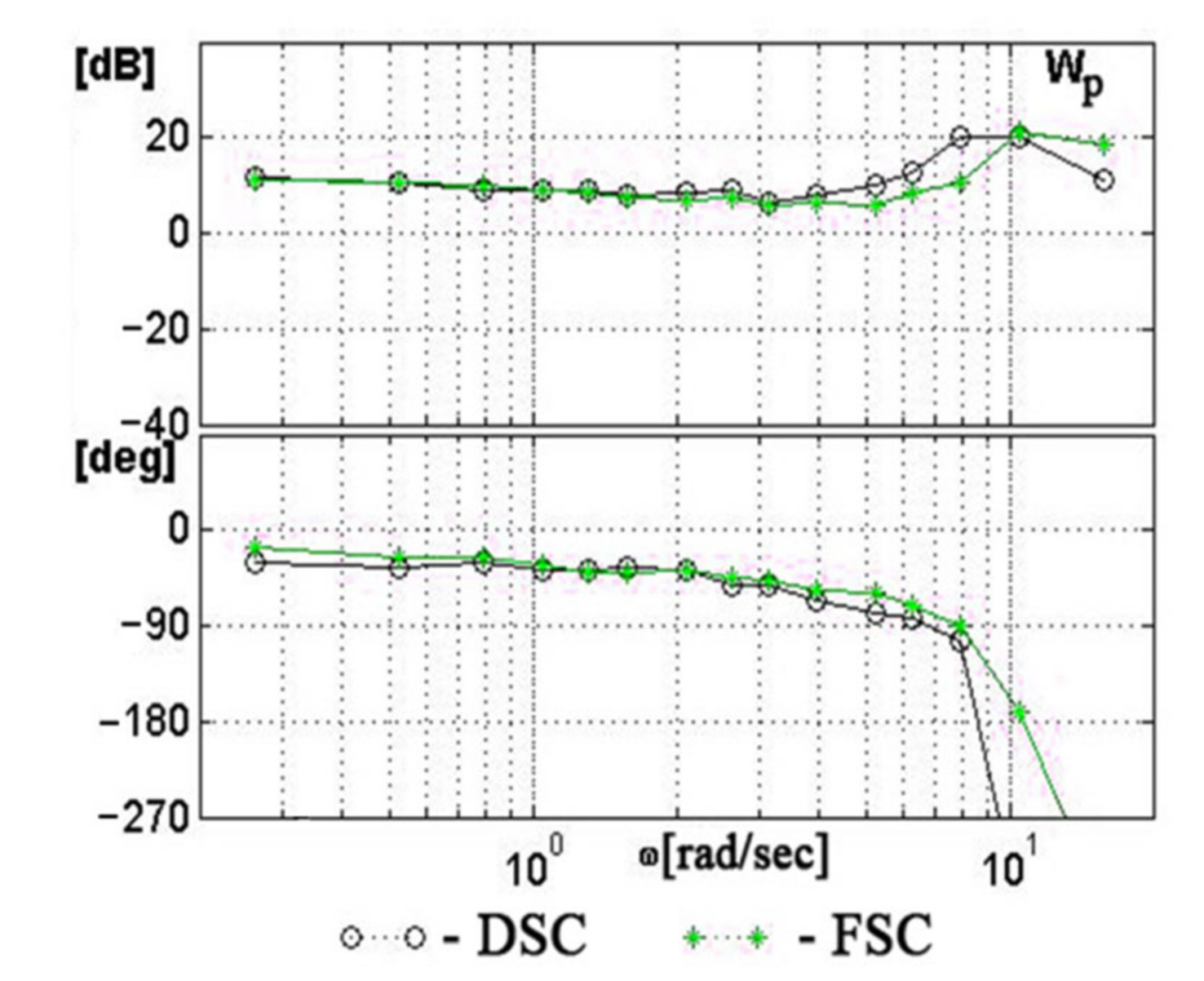
Figure 6 allows the study of a pilot–aircraft system for two types of pilot output signals: the displacement signal, performing the so-called “displacement sensing control (DSC)”, and the signal proportional to the force applied by the pilot, performing the so-called “force sensing control (FSC)” [30].

4.2. Ground-Based Simulations

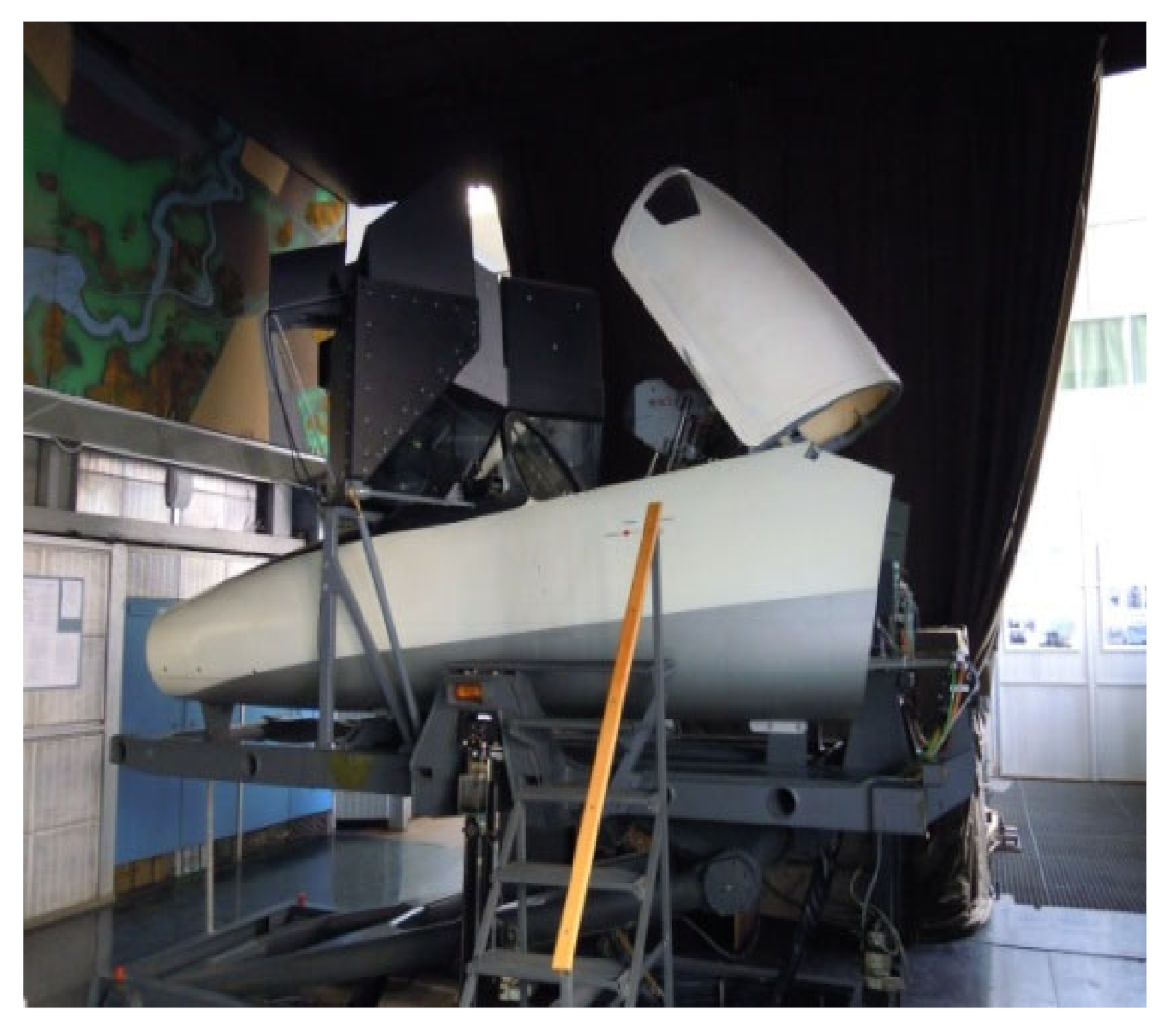
The effectiveness of inverse dynamics and the H∞ controller were also studied using a ground-based simulator equipped with a collimated visual system and the Moog control loading system (see Figure 7), as well as a workstation for the flying qualities studies.
An image of the compensatory display was shown on the screen of the central collimator. The vertical motion of the indicator on this display allowed us to perform a compensatory pitch tracking task. The Moog system equipped with force and displacement sensors made it possible to evaluate the effectiveness of the DSC and FSC types of pilot output.
The experiments involved two operators and one licensed pilot. They all had sufficient experience in ground-based simulations. The compensatory pitch tracking task was carried out with a polyharmonic input signal i t = k = 1 15 A k cos ω k t , which appeared as a random signal to the operators. Its amplitude Ak and orthogonal frequencies ω k = K 2 π T , where T is the duration of the trials, were selected from the requirements of correspondence between the power distributions of the polyharmonic signal and a random signal characterized by the spectral density S ii = K 2 ( ω 2 + 0 . 5 2 ) 2 ,   σ i 2 = 4   cm 2 .
The Fourier coefficient technique [31] was used for the calculation of the main pilot–vehicle system characteristics:
  • Pilot Wp(jω), open-loop WOL(jω) and closed-loop Φ ( j ω ) describe functions;
  • Pilot remnant spectral density S n e n e ( ω ) ;
  • Variance of error σ e 2 and its components σ e i 2 , which is the variance of error correlated with the input signal, and σ e n 2 , which is the variance of error correlated with the remnant.
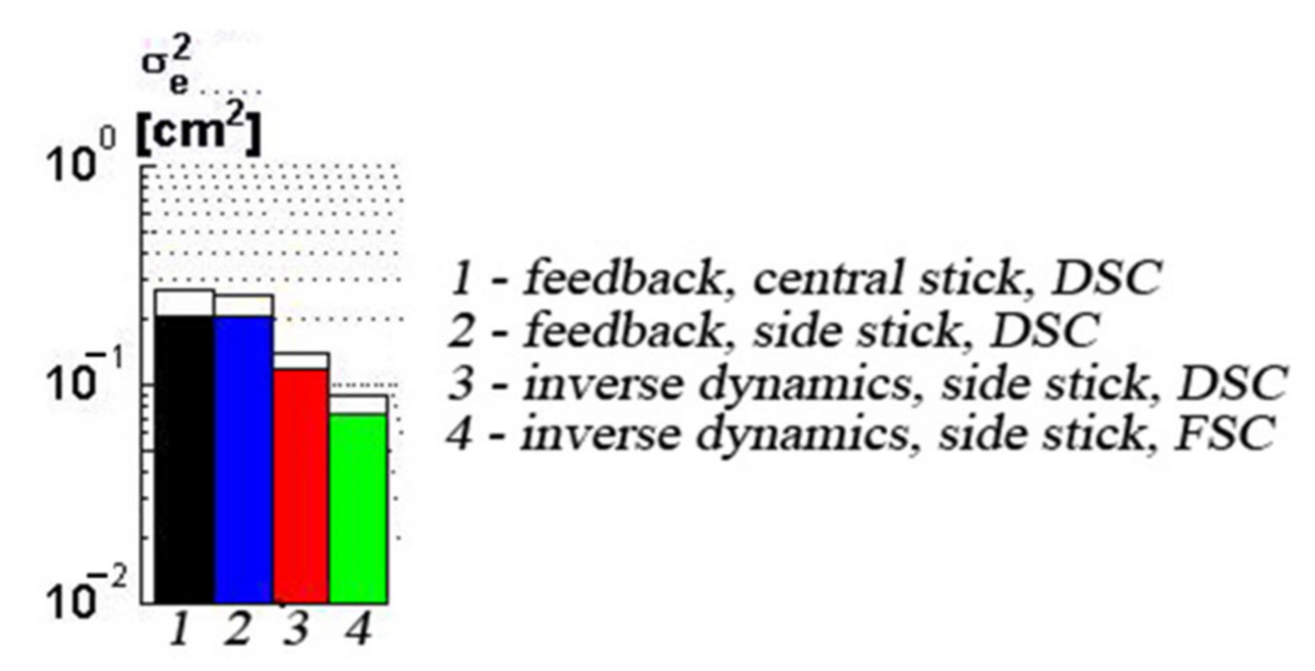
The experiments were carried out with two types of inceptors: a center stick and a sidestick.
At least three trials were executed for each variable (controlled element dynamics, type of inceptor and pilot output), and the obtained results were averaged. The duration of each trial was equal to 144 s.
The following controlled element dynamics W C were used in the experiments:
W C = W fb : dynamics of a controlled element whose control system consists of simple feedback gains only.
W C = W inv : dynamics of a controlled element whose control system includes feedback gains and inverse dynamics with a PI controller and filters F(s).
W C = W Hinf : dynamics of a controlled element whose control system is based on the H-infinity technique.

5. Investigation Results

The results of the ground-based simulations carried out for the three types of flight control systems—based on the use of traditional feedback gains only ( W C = W fb ), the inverse dynamics principle ( W C = W inv ) and the H-infinity technique ( W C = W inf )—are shown in Figure 8. The analysis of these results demonstrates that the use of inverse dynamics makes it possible to decrease the variance of error by a factor of 2.3 in comparison with feedback gains and by a factor of 1.5 in comparison with the H-infinity controller.
Qualitatively, similar results were also obtained in the mathematical modeling of the feedback- and inverse dynamics-based controller systems [14].

5.1. Time Response and Actuator Constraints

More intricacies of the inverse dynamics-based controller and H-infinity can be seen via the time response to a step input command in Figure 9. The helicopter model is used here without an actuator. It can be seen that the controller based on inverse dynamics has a faster rise time compared to the controller based on H-infinity. The slower rise time can also be seen in Figure 8, where the frequency response of the controlled element with an H-infinity controller has a phase drop that is more pronounced. All of this explains the high error variance of the H∞-based controller.
Another set of experiments was completed with a nonlinear actuator, where the actuator gain was set to 50, the rate limit set to 15 deg/s and the actuator deflection limit set to 25 deg. The results are shown in Figure 10. With the limitations set, it is easy to see that the inverse dynamics controller still provides a variance of error lower than that of the H-infinity controller by a factor of 1.25.
To simulate a worse actuator, the gain was reduced to 10, and the actuator limits were kept the same. As can be seen in Figure 11, in this setting, the performance is almost the same for both the inverse dynamics and the H-infinity controller.
Even though the frequency response characteristics are almost the same, it is seen that the H-infinity controller has a quicker phase drop at high frequencies, which introduces some delays. This can be seen reflected in the variance of error. Additionally, the implementation of an H-infinity controller is more complicated and requires extensive tuning. This tuning is reflected in choosing the parameters of the shaped system such that the maximum eigenvalues of the solutions to the Riccati equations are not complex. For this research, an automated cron job was run to evaluate several parameters and save the parameters that did not result in complex maximum eigenvalues, effectively creating a parameter space from which to choose parameters. This can also be carried out manually (see Section 3.3.).

5.2. Robustness

Since inverse dynamics is used in a feedforward control loop, it suffers from a lack of robustness. A simple PI controller was found to provide robustness by maintaining relatively good performance in the presence of modeling uncertainties. The results of the mathematical modeling shown in Figure 12 were obtained for the case when uncertainties were simulated by reducing all the coefficients of matrix B by 25% and increasing all the coefficients of matrix A by 50% of their nominal values.
To further examine the issue of robustness, ground-based experiments were also carried out for both the inverse dynamics and the H-infinity controllers. As seen in Figure 13, it was found that a simple PI controller added to the inverse dynamics controller was much more successful in providing robustness than the H-infinity controller.
Based on the experimental results shown above, it can be seen that the controller synthesized with inverse dynamics and a proportional-integral element was a much better controller by all metrics. It was therefore chosen as the default controller for the rest of this paper.

5.3. Flying Qualities Evaluation

Both the pilot describing function and the frequency response of the closed-loop system were calculated. This allowed us to calculate the parameters of the tentatively called “new MAI criterion for flying qualities prediction” [32]. This criterion is used as it is shown to have a high percentage of correct prediction of flying qualities levels.
This criterion is defined in terms of the following parameters:
  • The bandwidth of the pilot–vehicle closed-loop system ( ω BW ) corresponds to the frequency at which the phase response of the closed-loop system is equal to −90 deg.
  • The pilot compensation parameter ( Δ φ max = φ p W C φ p W C ) is calculated in the entire frequency range as the maximum difference between the pilot phase response of the investigated dynamics ( W C ) and that of the dynamics ( W C ), which do not require any pilot phase compensation (phase response corresponding to a time delay element ( W p = K p e j ω τ )).
The values of these parameters, calculated through mathematical modeling of the pilot–aircraft system for the controlled element dynamics where the controller is based on simple feedback gains and where it is based on inverse dynamics, are given in Figure 14.
The results shown in Figure 14 demonstrate that the use of inverse dynamics improves the flying qualities, making them correspond to the first level.
In the case where the control system is based on feedback gains only, the flying qualities belong to the second level.
The evaluation of flying qualities using the Bandwidth / Time Delay criterion from ADS-33E-RPF for the same dynamics did not reveal the fact that the investigated dynamics belong to different levels.
More experiments were carried out to evaluate the effects of inverse dynamics with different types of inceptors (center stick and sidestick) on the pilot–aircraft system characteristics. The research demonstrated that for both the center stick and sidestick, the pilot lead compensation is lower for the DSC type of pilot output. As an example, Figure 15 demonstrates the pilot frequency response obtained for the sidestick with both the DSC and FSC types of pilot output.
In addition, the use of a sidestick demonstrated a decrease in the variance of error σ e 2 in the case where the DSC type of pilot output and a traditional type of flight control system ( W C = W fb ) were used.
The variance of error σ e 2 decreases by a factor of 1.1 to 1.3 (see Figure 16). The same consistencies were obtained in [28] for different aircraft dynamics configurations.
The experiments conducted for inverse dynamics with the same type of inceptor and pilot output demonstrated a decrease in the variance of error by an additional factor of 1.8. When the FSC type of pilot output was used, the variance of error decreased even more, by an additional factor of 1.55. These results are shown in Figure 16.
The shortcoming of the FSC type of sidestick is the relatively higher rates of inceptor deflections in comparison with the DSC type of sidestick (see Figure 17).
This can cause errors in tracking tasks and increase the probability of PIO. This shortcoming can be eliminated with the help of a prefilter. The effect of an added non-linear prefilter is shown in Figure 18.

6. Discussion

This paper went through the development of control algorithms based on the inverse dynamics technique and the H-infinity technique for flight control. During the development of the latter, a filter based on the inverse dynamics was introduced in order to provide better performances to the H-infinity-based controller. One thing that stood out was that even though theoretically this technique seems easy and straight forward, its implementation was rather difficult, as singularities appeared in the application of the algorithms for certain parameters. Moreover, this required additional optimization loops to find the right parameters.
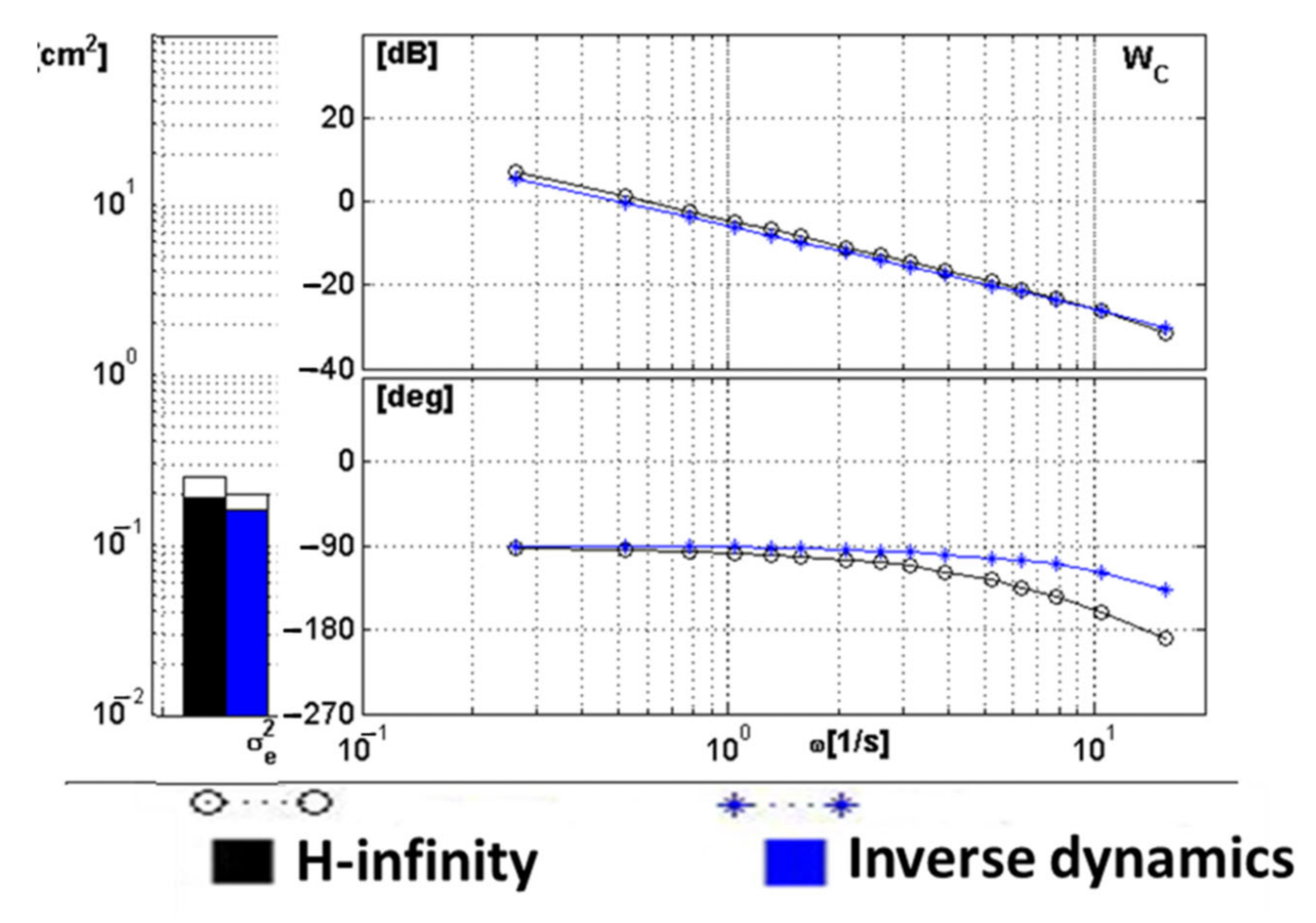
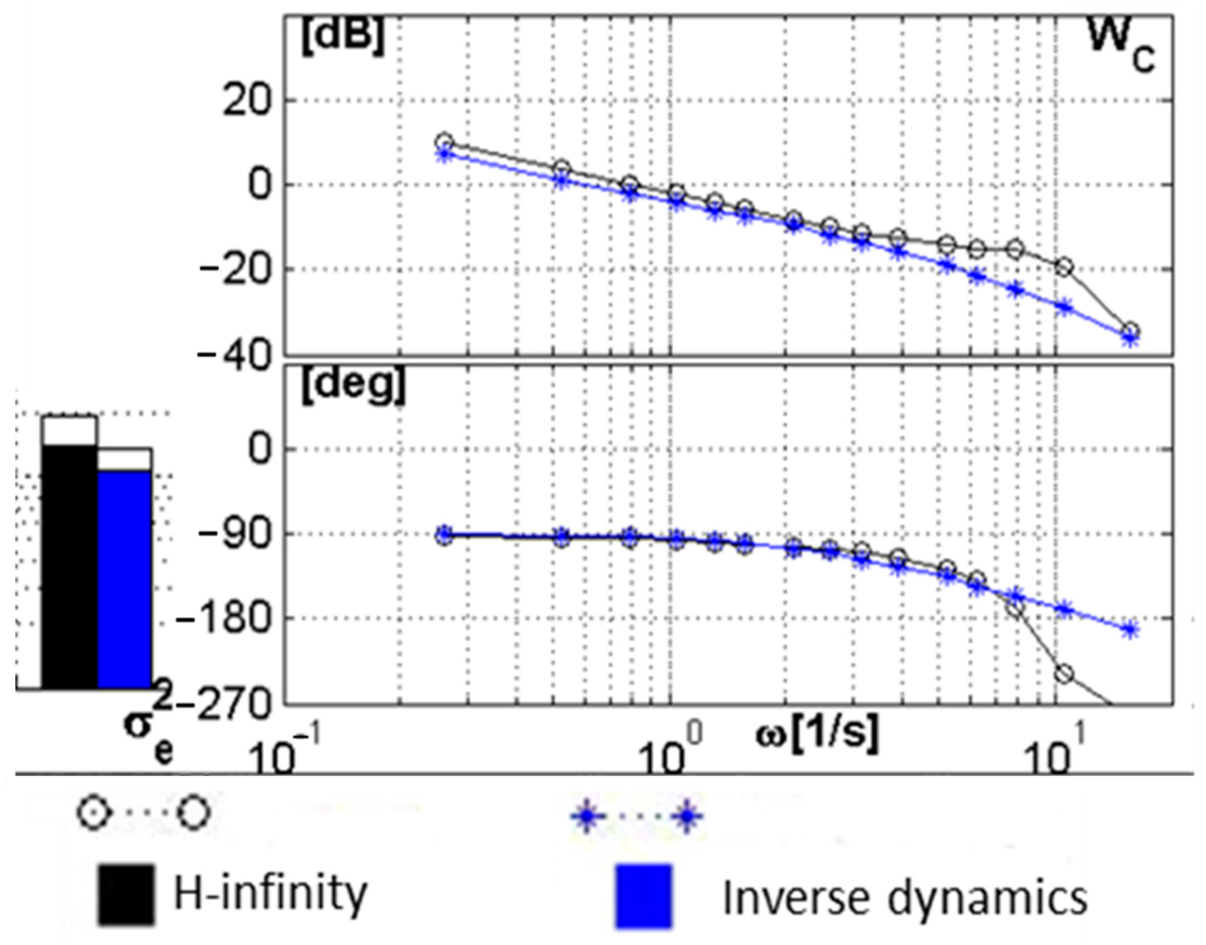
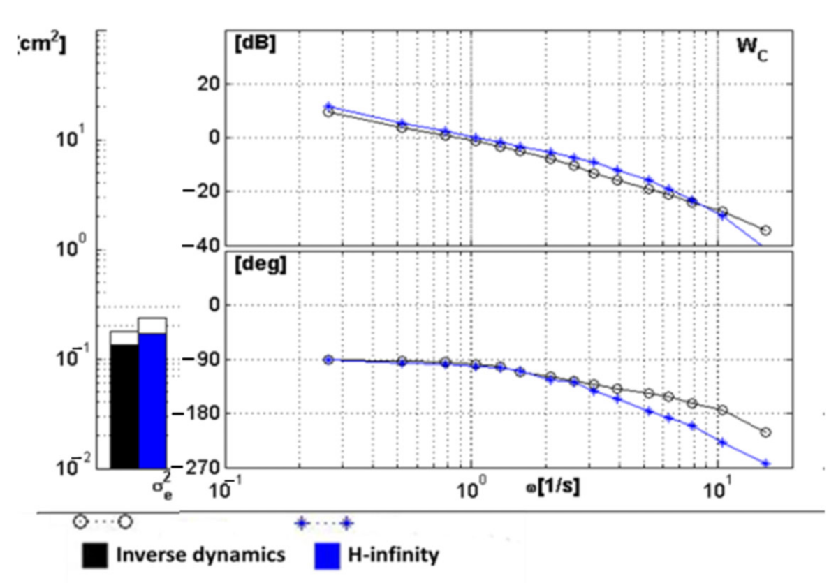
A comparative study was carried out between the traditional feedback gains, the inverse dynamics controller and the H-infinity-based controller. This study revealed that both the H-infinity controller and the inverse dynamics controller provided much better performances compared to the traditional feedback gains, with the variance of error decreasing by a factor of up to 2.3 times. At the same time, the inverse dynamics controller proved to be better than the H-infinity controller, even with degraded actuators. This is mostly because the H-infinity-based controller has a sensitive fundamental tradeoff between performances and robustness.
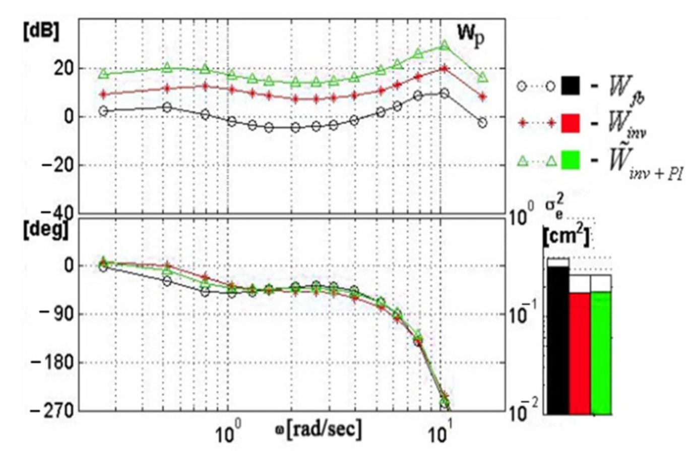
The lack of robustness of the inverse dynamics controller was solved by introducing a PI controller, which came as an addition to the good performances of the inverse dynamics without degrading them. This gave an upper hand to this controller.
To evaluate the robustness characteristics, uncertainties were introduced in the mathematical model of the vehicle used by changing the coefficients of both the state matrix and input matrix. Moreover, ground-based simulations showed that the inverse dynamics equipped with a PI controller were much better at handling uncertainties than the H-infinity controller, with the variance of error decreasing by a factor of up to 2.
Different control sticks and different control signals were also investigated to find their best integration with the control algorithms. This investigation revealed that using a sidestick, along with force sensing control (FSC), which sends control signals proportional to the force applied on the stick by the pilot, provides much better performance than any other combination, with the variance of error decreasing by up to 3.9 times in comparison with the traditional feedback gains.
One problem that arises when using inverse dynamics is the high actuator rates that are increased even more when the FSC type of output is used. This problem was solved by introducing a nonlinear prefilter between the pilot signals and the flight control system. This allowed a considerable decrease in the actuator rates, while maintaining good performances.
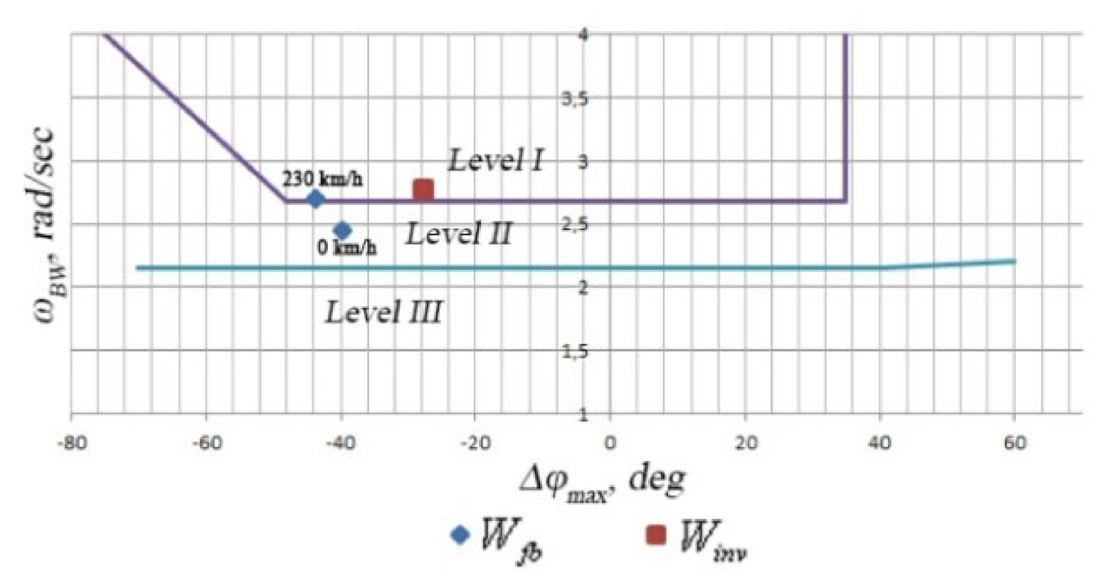
Another aspect considered in this paper is flying qualities requirements. To estimate the flying qualities provided by the controllers developed, the new Mai criterion was used. This criterion revealed that the inverse dynamics controller provides flying qualities of level 1 in all the flight conditions.

7. Conclusions

Control techniques were developed by using the inverse dynamics and H-infinity principles and were compared to a fight control system based on the use of feedback gains only. The proposed algorithms are general control design techniques that can be applied to both fixed-wing aircrafts and rotorcrafts. In this work, the effectiveness of the techniques is studied using a helicopter.
The implementation of inverse dynamics and the need for robustness required the installation of filters F(s), to make the inverse dynamics proper, and PI controllers in the flight control system.
The experimental investigations demonstrated a higher efficiency when using inverse dynamics in comparison with H-infinity, which is also more efficient than feedback gains only. Comparative studies also showed that an H-infinity controller with an inverse dynamics filter provides performance close to that of an inverse dynamics controller when the actuator is degraded. However, the difficulty and complexity of implementing and tuning the H-infinity controller makes it much less appealing compared to the inverse dynamics-based one. Therefore, for this study, the inverse dynamics-based controller was chosen for further experimentation. These investigations showed that its integration with a sidestick and the force sensing control type of pilot output makes it possible to increase performances in comparison to the traditional flight control system with feedbacks, a center stick and the DSC type of pilot output. Additionally, the technique developed in this paper allowed us to decrease the pilot phase delay in the high-frequency range. The high actuator rate demand of the sidestick with FSC, which can be seen as a shortcoming, can be eliminated by using a nonlinear prefilter between the pilot commands and the control system.

Author Contributions

Conceptualization, A.V.E., Z.M. and E.V.E.; methodology, A.V.E., Z.M. and E.V.E.; software, Z.M. and E.V.E.; validation, A.V.E., Z.M. and E.V.E.; formal analysis, A.V.E. and Z.M.; investigation, A.V.E., Z.M. and E.V.E.; resources, A.V.E.; data curation, Z.M. and E.V.E.; writing—original draft preparation, Z.M.; writing—review and editing, A.V.E. and Z.M.; visualization, Z.M. and E.V.E.; supervision, A.V.E.; project administration, A.V.E.; funding acquisition, A.V.E. All authors have read and agreed to the published version of the manuscript.

Funding

This research was funded by the Russian Ministry of Science and Higher Education, grant number 075-15-2020-924.

Institutional Review Board Statement

Not applicable.

Informed Consent Statement

Not applicable.

Data Availability Statement

The data presented in this study are available on request from the corresponding author. The data are not publicly available due to privacy reasons.

Acknowledgments

The paper is prepared in the framework of the Program for the Development of a World-Class Research Center “Supersonic” in 2020-2025 funded by the Russian Ministry of Science and Higher Education (Agreement dated 16 Nov 2020 № 075-15-2020-924).

Conflicts of Interest

The authors declare no conflict of interest, and the funders had no role in the design of the study; in the collection, analyses, or interpretation of data; in the writing of the manuscript; or in the decision to publish the results.

References

  1. Padhi, R.; Rao, P.N.; Goyal, S.; Balakrishnan, S.N. Command tracking in high performance aircrafts: A new dynamic inversion design. IFAC Proc. 2007, 40, 79–84. [Google Scholar] [CrossRef] [Green Version]
  2. Chen, H.B.; Zhang, S.G. Robust Dynamic Inversion Flight Control Law Design. In Proceedings of the 2008 2nd International Symposium on Systems and Control in Aerospace and Astronautics, Shenzhen, China, 10–12 December 2008; pp. 1–6. [Google Scholar]
  3. Horn, J.F. Non-Linear Dynamic Inversion Control Design for Rotorcraft. Aerospace 2019, 6, 38. [Google Scholar] [CrossRef] [Green Version]
  4. Ma, S.; Yang, G. Helicopter Nonlinear Dynamic Inversion Flight Control Model Design. In Proceedings of the 2016 International Conference on Control, Automation and Information Sciences (ICCAIS), Ansan, Korea, 27–29 October 2016; pp. 155–161. [Google Scholar]
  5. Zhao, Y.; Jayasuriya, S. Feedforward Controllers and Tracking Accuracy in the Presence of Plant Uncertainties. In Proceedings of the 1994 American Control Conference—ACC ’94, Baltimore, MD, USA, 29 June–1 July 1994; Volume 1, pp. 360–364. [Google Scholar]
  6. Devasia, S. Robust Inversion-Based Feedforward Controllers for Output Tracking under Plant Uncertainty. In Proceedings of the 2000 American Control Conference, ACC (IEEE Cat. No.00CH36334), Chicago, IL, USA, 28–30 June 2000; Volume 1, pp. 497–502. [Google Scholar]
  7. Devasia, S. Should Model-Based Inverse Inputs Be Used as Feedforward under Plant Uncertainty? IEEE Trans. Aut. Control 2002, 47, 1865–1871. [Google Scholar] [CrossRef] [Green Version]
  8. Brinker, J.S.; Wise, K.A. Stability and Flying Qualities Robustness of a Dynamic Inversion Aircraft Control Law. J. Guid. Control Dyn. 1996, 19, 1270–1277. [Google Scholar] [CrossRef]
  9. Ansari, U.; Bajodah, A.H. Robust Generalized Dynamic Inversion Based Control of Autonomous Underwater Vehicles. Proc. Inst. Mech. Eng. Part M J. Eng. Marit. Environ. 2018, 232, 434–447. [Google Scholar] [CrossRef]
  10. Peng, C.; Han, C.; Zou, J.; Zhang, G. H ∞ Optimal Inversion Feedforward and Robust Feedback Based 2DOF Control Approach for High Speed-Precision Positioning Systems. J. Control Sci. Eng. 2016, 2016, 1–11. [Google Scholar] [CrossRef] [Green Version]
  11. Kondrat’ev, A.I.; Tyumentsev, Y.V. Application of Neural Networks for Synthesizing Flight Control Algorithms. I Neural Network Inverse Dynamics Method for Aircraft Flight Control. Russ. Aeronaut. 2013, 56, 135–144. [Google Scholar] [CrossRef]
  12. Miller, C.J. Nonlinear Dynamic Inversion Baseline Control Law: Architecture and Performance Predictions. In Proceedings of the AIAA Guidance, Navigation, and Control Conference, Portland, OR, USA, 8–11 August 2011. [Google Scholar]
  13. Mbikayi, Z.; Efremov, A.V.; Efremov, E.V. Integration of the Inverse Dynamics with a Reference Model Technique, and Its Application for the Improvement of the Helicopter Flying Qualities. IOP Conf. Ser. Mater. Sci. Eng. 2020, 868, 012016. [Google Scholar] [CrossRef]
  14. Efremov, A.V.; Efremov, E.V.; Mbikayi, Z.; Esaulov, S.Y.; Ivchin, V.A.; Myasnikov, M.I. Synthesis of a Helicopter Control System Using Inverse Dynamics and Its Upgrade with the Use of a Sidestick Controller. In Proceedings of the European Rotorcraft Forum, ERF—2020, Moscow, Russia, 8–11 September 2020; pp. 9–17. [Google Scholar]
  15. Zames, G. Feedback and Optimal Sensitivity: Model Reference Transformations, Multiplicative Seminorms, and Approximate Inverses. IEEE Trans. Autom. Control 1981, 26, 301–320. [Google Scholar] [CrossRef]
  16. Nichols, R.A.; Reichert, R.T.; Rugh, W.J. Gain Scheduling for H-Infinity Controllers: A Flight Control Example. IEEE Trans. Control Syst. Technol. 1993, 1, 69–79. [Google Scholar] [CrossRef] [Green Version]
  17. Ashok Kumar, B.; Gayathri, S.; Surendhar, S.; Senthilrani, S.; Jeyabharathi, R. Robust H-Infinity Controller for Two Degree of Freedom Helicopter. In Proceedings of the 2019 IEEE International Conference on System, Computation, Automation and Networking (ICSCAN), Pondicherry, India, 29–30 March 2019; pp. 1–5. [Google Scholar]
  18. Nair, V.V.; Jayasree, P.R.; Parvathy, G. Robust Control of Helicopter with Suspended Load. In Proceedings of the 2017 International Conference on Circuit, Power and Computing Technologies (ICCPCT), Kollam, India, 20–21 April 2017; pp. 1–6. [Google Scholar]
  19. McFarlane, D.; Glover, K. A Loop-Shaping Design Procedure Using H/Sub Infinity/Synthesis. IEEE Trans. Autom. Control 1992, 37, 759–769. [Google Scholar] [CrossRef]
  20. Azar, A.T.; Serrano, F.E.; Kamal, N.A. Robust H∞ Loop Shaping Controller Synthesis for SISO Systems by Complex Modular Functions. Math. Comput. Appl. 2021, 26, 21. [Google Scholar] [CrossRef]
  21. Geng, L.; Yang, Z.; Zhang, Y. A Weighting Function Design Method for the H-Infinity Loop-Shaping Design Procedure. In Proceedings of the 2018 Chinese Control and Decision Conference (CCDC), Shenyang, China, 9–11 June 2018; pp. 4489–4493. [Google Scholar]
  22. Smit, M.; Craig, I. Robust flight controller design using H-infinity loop-shaping and dynamic inversion techniques. In Guidance, Navigation, and Control Conference and Exhibit; American Institute of Aeronautics and Astronautics: Boston, MA, USA, 1998. [Google Scholar]
  23. Schumacher, C.J. Tactical Missile Autopilots: Gain-Scheduled H(Infinity) Control and Dynamic Inversion. Ph.D. Thesis, University of Michigan, Ann Arbor, MI, USA, 1997. [Google Scholar]
  24. Buchholz, J.J.; von Grünhagen, W. Inversion Impossible? GRIN Publishing: Munich, Germany, 2003. [Google Scholar]
  25. Tailor, M.R.; Bhathawala, P.H. Linearization of Nonlinear Differential Equation by Taylor’s Series Expansion and Use of Jacobian Linearization Process. Int. J. Theor. Appl. Sci. 2011, 4, 36–38. [Google Scholar]
  26. Glover, K.; McFarlane, D. Robust Stabilization of Normalized Coprime Factor Plant Descriptions with H_infinity-Bounded Uncertainty. IEEE Trans. Aut. Control 1989, 34, 821–830. [Google Scholar] [CrossRef]
  27. Vidyasagar, M. Control System Synthesis: A Factorization Approach; Massachusetts Institute of Technology: Cambridge, MA, USA, 1985; ISBN 9780262220279. [Google Scholar]
  28. Efremov, A.V.; Aleksandrov, V.V.; Efremov, E.V.; Vukolov, M.V. The Influence of Different Types of Inceptors and Their Characteristics on the Pilot-Aircraft System. IFAC-Pap. 2019, 51, 372–377. [Google Scholar] [CrossRef]
  29. Efremov, A.V. Pilot-Aircraft System. Regularities and Mathematical Models of Pilot Behavior; MAI: Moscow, Russia, 2017. [Google Scholar]
  30. Klyde, D.H.; McRuer, D. Smart-Cue and Smart-Gain Concepts to Alleviate Loss of Control. J. Guid. Control Dyn. 2009, 32, 1409–1417. [Google Scholar] [CrossRef]
  31. Efremov, A.V.; Rodchenko, V.V.; Boris, S. Investigation of Pilot Induced Oscillation Tendency and Prediction Criteria Development; WL-TR-96-3109; Wright Laboratory: Dayton, OH, USA, 1996; pp. 1–138. [Google Scholar]
  32. Efremov, A.; Efremov, E.; Tiaglik, M. Advancements in Predictions of Flying Qualities, Pilot-Induced Oscillation Tendencies, and Flight Safety. J. Guid. Control Dyn. 2020, 43, 4–14. [Google Scholar] [CrossRef]
Figure 1. Using inverse dynamics.
Aerospace 08 00290 g001
Figure 2. Inverse dynamics vs. feedback.
Aerospace 08 00290 g002
Figure 3. Shaped system.
Aerospace 08 00290 g003
Figure 4. Controller implementation.
Aerospace 08 00290 g004
Figure 5. Pilot–aircraft system.
Aerospace 08 00290 g005
Figure 6. Modified pilot structural model.
Aerospace 08 00290 g006
Figure 7. Ground-based simulator.
Aerospace 08 00290 g007
Figure 8. Experimental results.
Aerospace 08 00290 g008
Figure 9. Controller comparison in pitch rate tracking.
Aerospace 08 00290 g009
Figure 10. Inverse dynamics vs. H-infinity with actuator constraints and high gain.
Aerospace 08 00290 g010
Figure 11. Inverse dynamics vs. H-infinity with actuator constraints and low gain.
Aerospace 08 00290 g011
Figure 12. Results of mathematical modeling with uncertainties.
Aerospace 08 00290 g012
Figure 13. Results of experiments with uncertainties.
Aerospace 08 00290 g013
Figure 14. New MAI criterion.
Aerospace 08 00290 g014
Figure 15. Pilot describing functions for DSC and FSC pilot output.
Aerospace 08 00290 g015
Figure 16. Variance of error.
Aerospace 08 00290 g016
Figure 17. Rate δ ( t ) ˙ of the control signal. (a) DSC, (b) FSC.
Aerospace 08 00290 g017
Figure 18. Effect of a non-linear prefilter. (a) function demonstration of nonlinear prefilter, (b) DSC, (c) FSC.
Aerospace 08 00290 g018
Publisher’s Note: MDPI stays neutral with regard to jurisdictional claims in published maps and institutional affiliations.

