1. Introduction
Technologies related to UAVs have become prominent in aircraft science and engineering because of the exploding civilian and military applications that are tailored around UAVs capabilities. Among these, it is worth mentioning applications such as military/law enforcement/civilian surveillance, patrolling and rescue operations, agriculture applications, goods/food delivery, aerial photography, and more. In addition, a huge interest in large electric multicopters for Urban Air Mobility has been observed in recent years.
There are two main categories of UAVs: Fixed-wing UAVs that are incapable of hovering and multi-rotor (i.e., rotary-wing) UAVs (that may consist of fixed-wing as well). This paper is focused on the latter that seems to have many advantages in low altitude and confined areas.
Parallel to this trend, the advancements in electric motor and improved batteries capacities led to the development of a vast range of multiple rotors applications in novel concepts.
Multirotor configurations also introduce strong aerodynamic, dynamic, aeroacoustic interactions and controllability issues that are not fully captured through traditional and conventional aircraft conceptual/preliminary design stages.
A more systematic approach is expected to provide better design performance and the possibility to rapidly assess the effect of changes in the mission requirements.
Hence, a tendency towards the adoption of higher fidelity analysis tools during the early sizing and preliminary design stages is observed in recent years. Nowadays, designers are equipped with many analysis tools of various fidelity levels. Yet, the tools used in the preliminary, conceptual, and optimization stages should be relatively simple and based on fast design cycles in which a vast range of effects of various components is examined. Hence, at such preliminary stages, designers typically tend to employ some semi-empirical design rules to construct a suitable working point for a new proposed configuration.
One of the tools usually used is generally characterized as “design trends”, in which existing flying configurations are analyzed to conclude or identify a trend that is common to many configurations. It is highly reasonable that such trends may represent some physical constraints that should be taken into account, but are not clear enough and evident in the early design stages. In such early phases, standard analysis tools are therefore less effective because detailed data of the configuration are not yet available.
Evaluation of historical design trends during the early sizing and preliminary design stages is a well-known tool for both fixed- and rotary-wing configurations, see Refs. [
1,
2,
3,
4,
5]. Such trends include performance and weight assessments and may be comprised of cost estimations as well. It should be noted that in principle, the notion “design trend” may also include configuration selection as this selection is highly connected to the mission type. Such trends are expected to be available in the future as information about more vehicles will be available.
Sizing and analysis of Multi-Prop/rotor UAVs are documented in the literature, see for example, Refs. [
6,
7,
8,
9,
10,
11,
12,
13,
14].
Analysis of design trends includes, in addition to the obvious geometrical sizing of the vehicle, some preliminary performance estimation including the required power, subsystems weight, battery characteristics, and so forth.
Besides the use of design trends, the present paper also offers a mission-oriented design scheme this is well-aligned with the requirement to include a medium fidelity and not computationally expensive analysis of the propellers interaction. This part is carried out by vortex filaments representation of the propeller’s wakes. The cost of this computation is well below the one required for fully CFD analysis and the resulting accuracy is enough for adequate performance analysis.
This paper is devoted to the sizing and preliminary analysis of Multi-Prop UAVs. Throughout the paper, we have chosen to use the terminology “propeller” over “rotor”. This selection is not very consistent and may be ambiguous in some cases. Yet, this choice was made as most of the rotary-wing devices on multi-prop vehicles are rotational-velocity controlled fixed-pitch propellers (as opposed to variable/cyclic pitch of rotors). However, as opposed to standard propellers for axial flight, the blades are designed with a much less (built-in) twist to accommodate efficient hover as well.
2. Design Trends
This section demonstrates some examples of statistical trends of sub-systems of multi-prop UAVs that were collected from the open literature, for example, Refs. [
15,
16,
17,
18,
19,
20,
21,
22,
23,
24,
25,
26,
27]. Part of these trends will be accompanied by the characteristics that were determined by RAPiD (Rotorcraft Analysis for Preliminary Design)—see Refs. [
28,
29,
30,
31]) using the numerical process described further on in this paper. One example is demonstrated throughout this paper where symbols of a cross-over-a-circle are RAPiD’s calculated results and symbols of a-cross-over-a-square indicate values that were taken from the design trend lines to facilitate the analysis.
Note that, intentionally, units were tuned for better clarity as most of the data in the literature are of a mixed nature (i.e., meters, millimeters, inches etc.) and, therefore, most of the numerical coefficients are dimensional.
To clarify the statistical analysis, it should be mentioned that all correlations were mathematically transformed into a linear regression scheme for which a correlation quality “R-squared’’ () has been determined and is indicated in the various graphs. The correlation coefficient, r, is an indication of the strength and direction of the relationships presented. However, the reliability of the model also depends on how many observed data points are in the sample. An additional hypothesis test of the “significance of the correlation coefficient” has been performed to decide whether the linear relationship in the sample data is strong enough to use to model the relationship in the “population”. Only correlations that passed the significant level of are presented in this paper.
2.1. Design Trend I: Propeller Diameter, Weight and Pitch
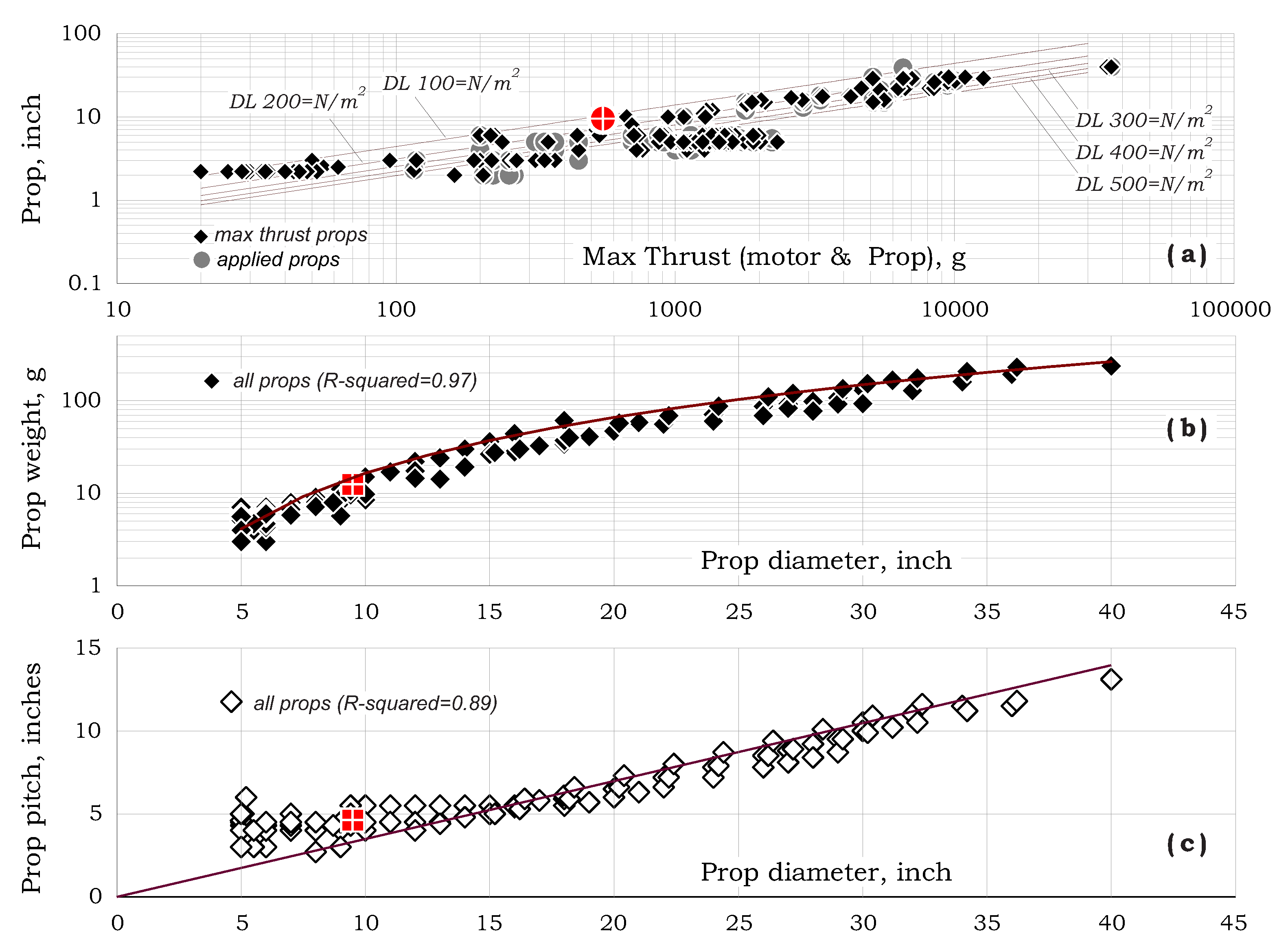
Figure 1a presents propeller diameter vs. max-thrust (the maximal thrust enabled by each prop-motor pair).
When described in logarithmic scales, the pattern suggests a general linear trend-line as expected for constant disc loading. Note that, by definition, propeller diameter as a function of thrust and disc loading may be written as:
The parallel lines in
Figure 1a were drawn using the above relation. As shown, most of the data appear to be spread around 300 N/m
, which is a value that is adopted by most designers. Propeller weight vs. diameter is shown in
Figure 1b by the trend-line
An effort to clarify the above relation calls for considering the blade as a thin-shell Carbon-Epoxy structure which allows the recreation of Equation (
2) as:
where
is the material density,
c is the average chord and
t is the (assumed constant) shell thickness. Using
and
1500 kg/m
, a typical average material thickness of about 0.81 mm is obtained by equating Equations (
2) and (
3).
Propeller pitch vs. diameter is shown in
Figure 1c by the trend-line
This value reflects relatively low pitch ratio (). Such a value is expected since multi-prop vehicles typically experience low normal-to-the-disc component of the incoming free-stream velocity inflow.
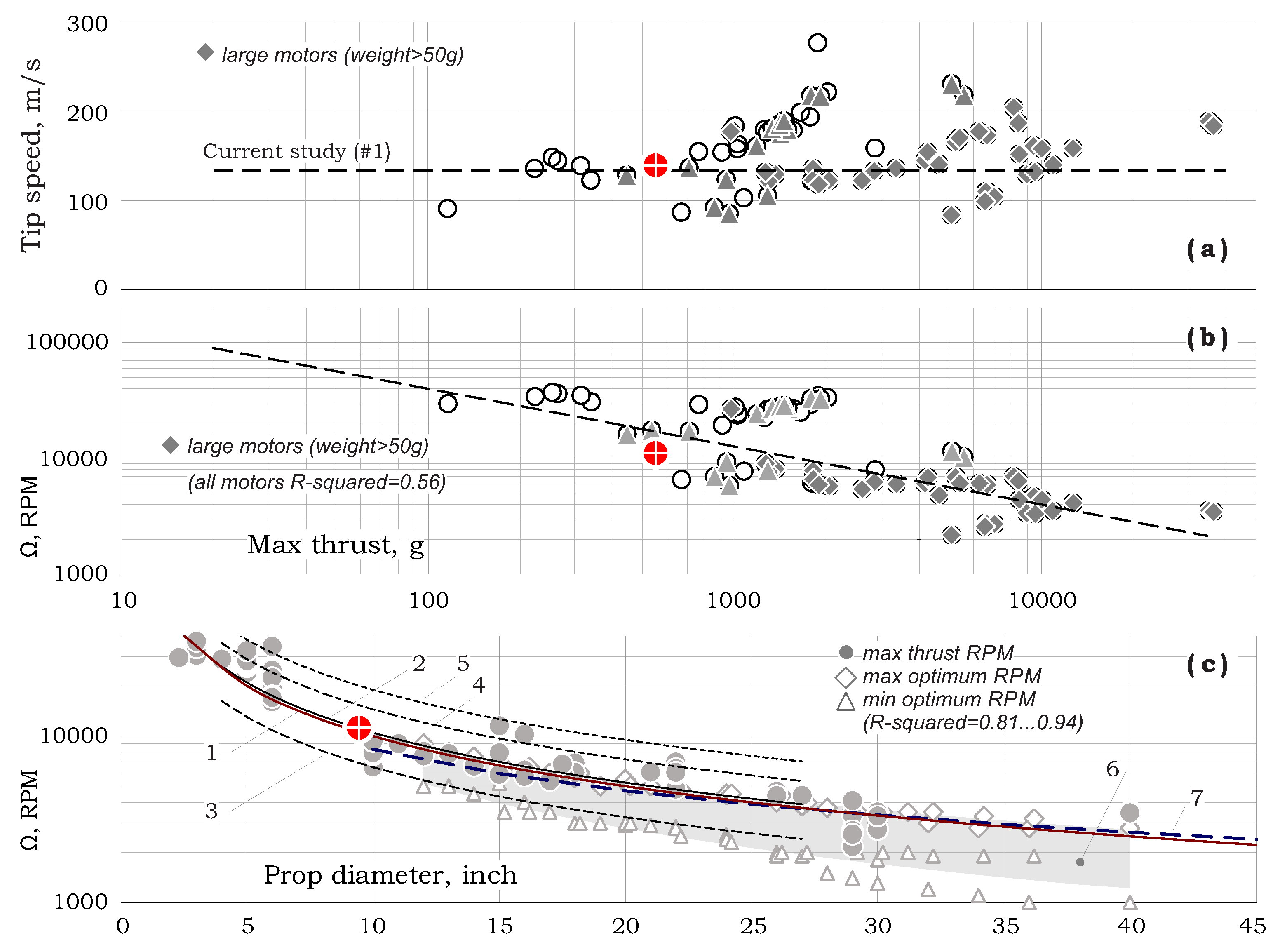
2.2. Design Trend II: Propeller Rotational Velocity
Figure 2a presents propeller tip velocity (
) vs. max-thrust.
As shown, for most propellers, tip velocity varies in the range of 100–200 m/s with low dependency on thrust level. However,
Figure 2b shows that the rotational velocity,
, decreases with increasing thrust levels as
The above may be used to connect the rotational velocity to the propeller diameter. This may be carried out by using Equation (
1) with
300 N/m
that yields the relation
. Hence, the variation of
with respect to the diameter shown in
Figure 2c may be predicted as:
(see line #1) which matches the horizontal line of
133 m/s in
Figure 2a.
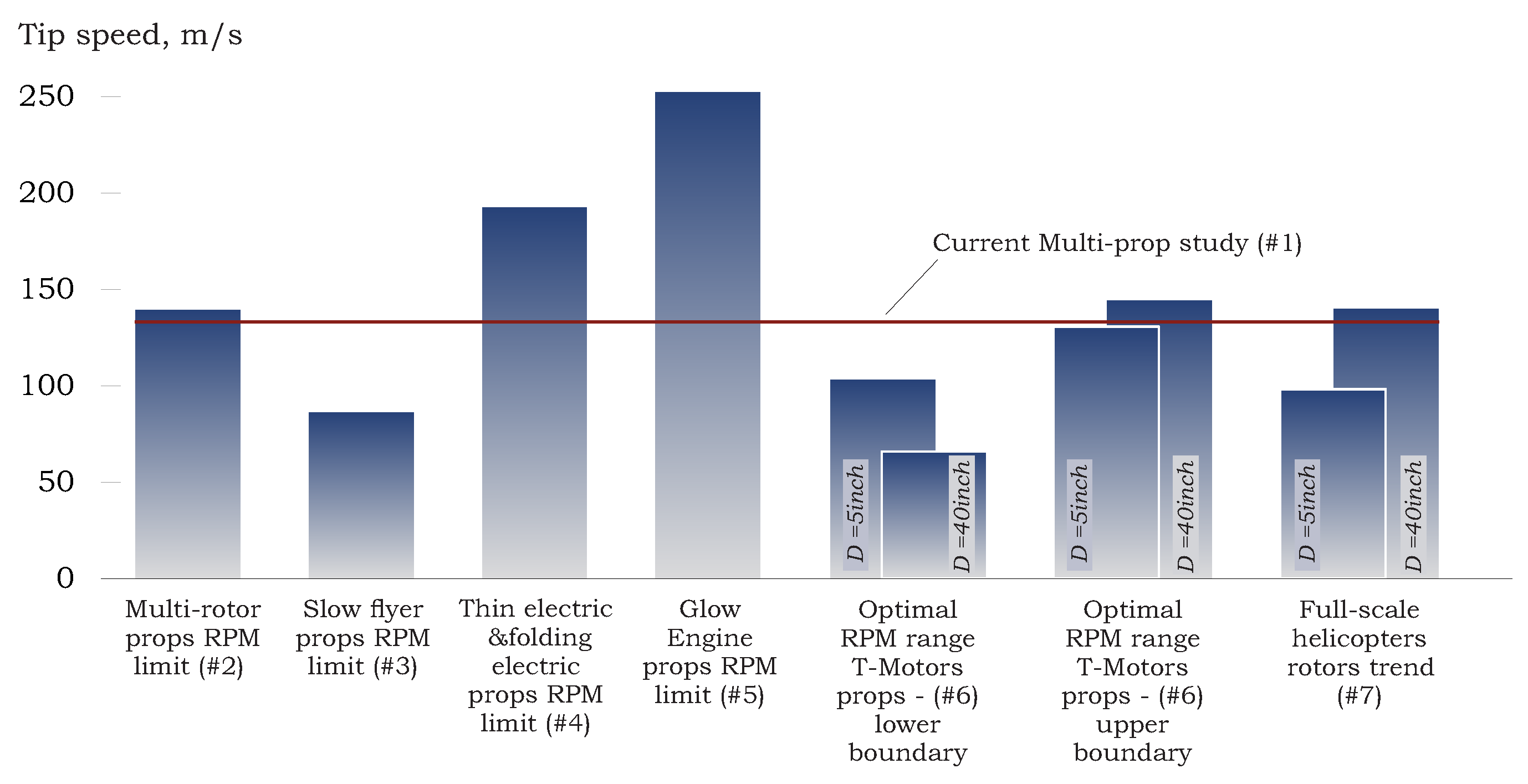
Reference [
15] presents tip velocity recommendations for APC propellers (#2–#5), while Ref. [
16] shows optimal RPM range for T-motors propellers (#6). These are described in
Figure 3 where the typical range for full-scale helicopters is also included (#7), see Ref. [
4].
As shown, apart from the glow engine (a type of small internal combustion engine that requires high RPM for better efficiency), all tip velocities, including those of full-scale helicopters are in the range described above.
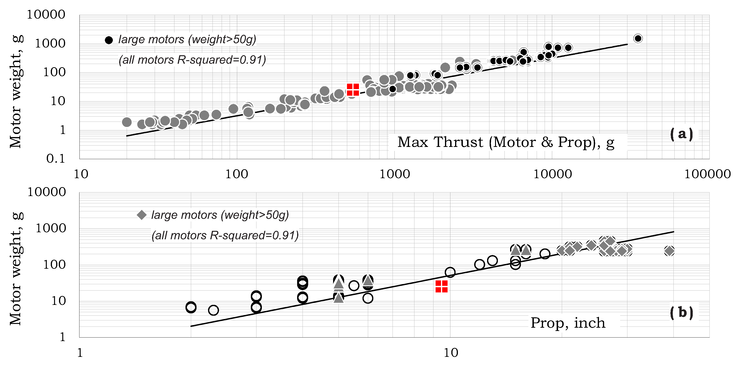
2.3. Design Trend III: Motor Characteristics
Figure 4a shows the design trend of motor weight vs. thrust.
This relation may be written as:
which is shown by the line in that figure. By using again Equation (
1) with
300 N/m
, Equation (
7) may be converted to
This trend is represented by the line in
Figure 4b and is consistent with the data shown.
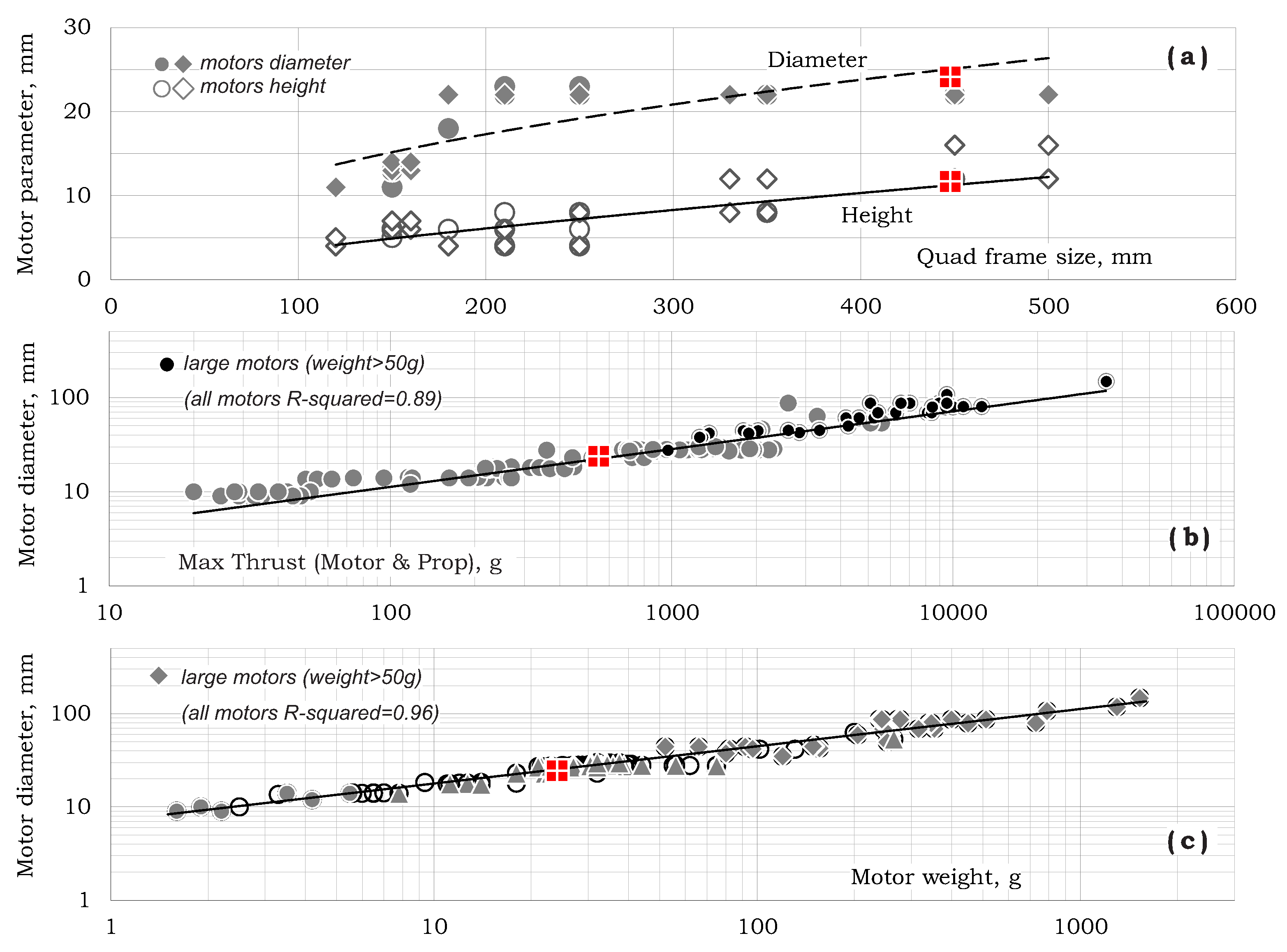
Figure 5 presents motor diameter as a function of the frame size, thrust, and motor weight. Typically, frame size is measured as the hub-to-hub distance. For a given number of propellers, it should be well correlated with the propeller’s diameter.
Figure 5a also presents motor height as a function of the frame size.
In general, a larger motor diameter (wider stator) provides more torque at lower RPM while a higher motor (taller stator) provides more power at higher RPM (see Refs. [
21,
22]). Nevertheless, both motor diameter and height were found to be well correlated with frame size as shown in
Figure 5a:
As shown in
Figure 5b, the motor diameter was also found to be correlated with max-thrust as
Using Equations (
7) and (
11), one may also describe the relation between motor diameter and motor weight as:
The latter is shown by the line in
Figure 5c that is well correlated with the data points.
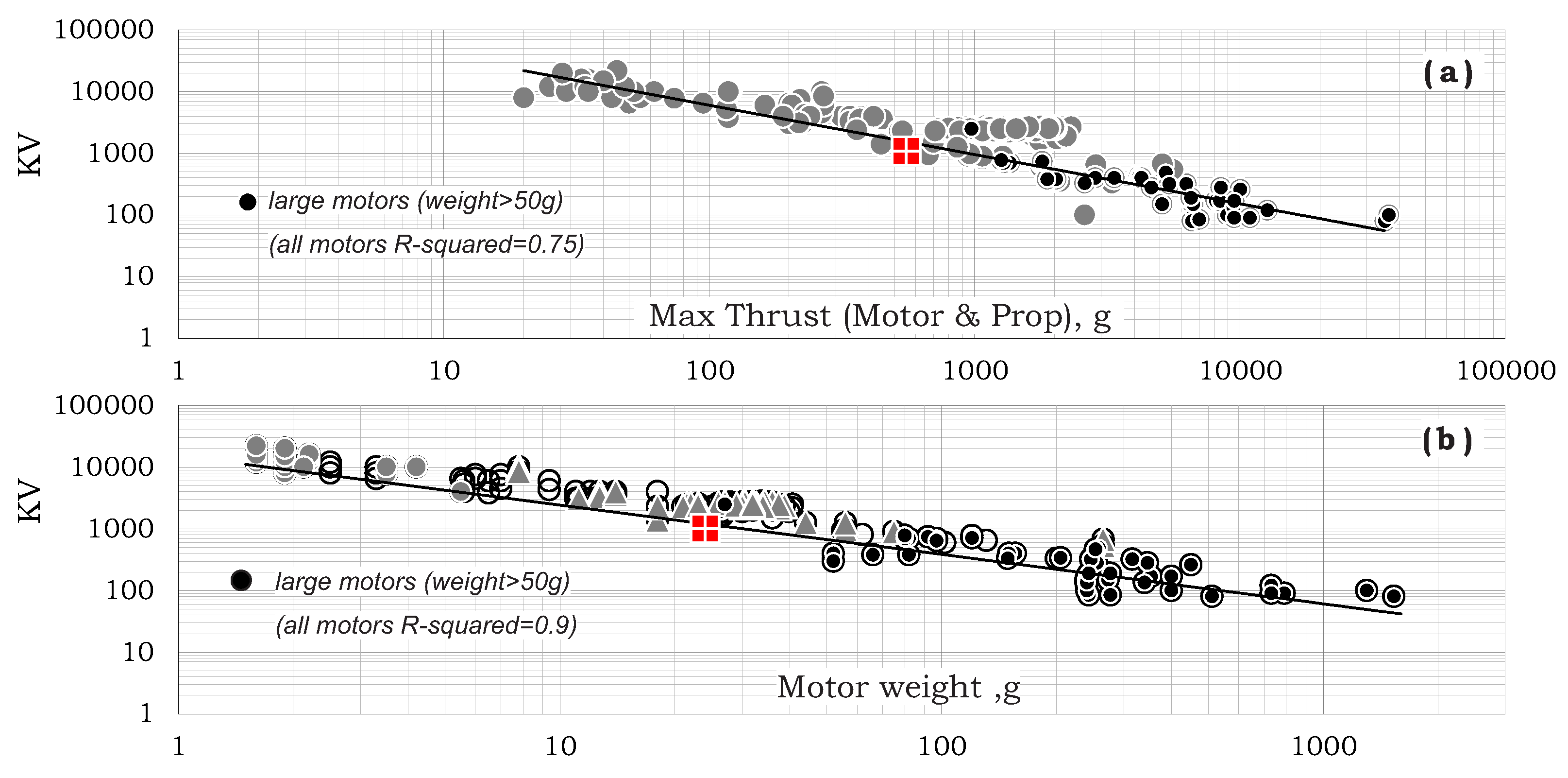
Figure 6 presents the design trend of the motors’ KV value (RPM per Volt of an unloaded motor).
As shown in
Figure 6a, motor
may be defined as a decreasing function of max-thrust:
which is shown by the line in that figure. Based on Equation (
7), one may also write:
which is represented by the line in
Figure 6b that is well correlated by the data. Note that higher
motors will create higher angular velocity while lower
motors will generate higher torque for a given voltage. Hence, larger propellers are paired with low
motors, while smaller and lighter propellers are paired with high
KV motors.
2.4. Design Trend IV: Motor & Propeller Operational Parameters
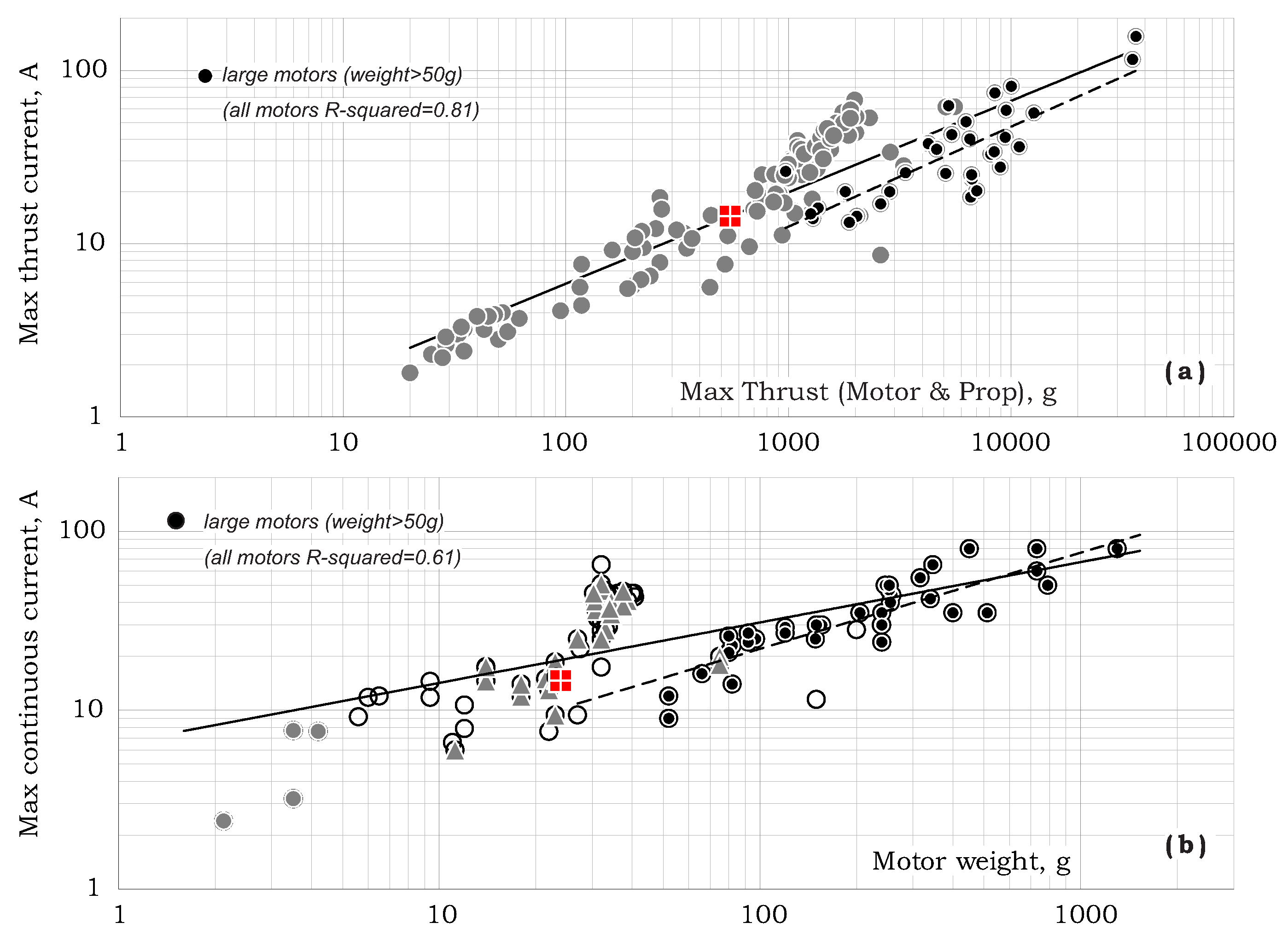
Figure 7 presents the total current consumption of a “motor-prop” systems vs. max-thrust and motor weight.
As shown, current consumption increases with both thrust and motor weight. The max-thrust current consumption for motor-prop system (the full line in
Figure 7a) is given by:
At the same time, current consumption for large motors are shown to be smaller (the dashed line in
Figure 7a). This trend may testify for a more efficient design that is enabled for larger motors.
The max-continuous current trend-line for all motors is shown by the full line in
Figure 7b as:
while again, the dashed line shows the max-continuous current for larger motors. Comparing the above two trends shows that, on average,
is smaller than
by 20%.
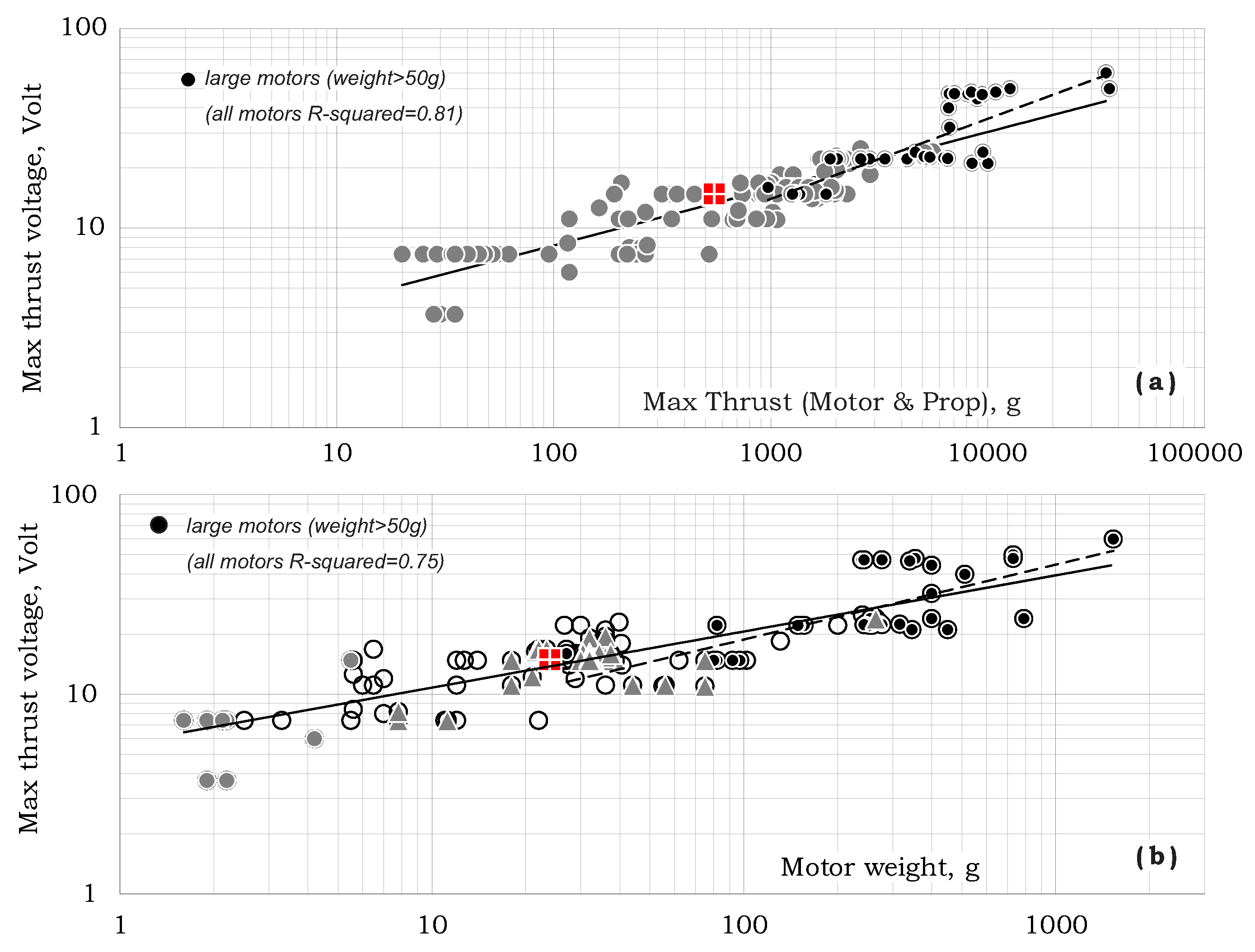
Figure 8 presents the system’s voltage vs. max-thrust and motor-weight.
Based on
Figure 8a, the design trend in this case turns out to be:
Considering all data in
Figure 8b, the dependency of the voltage in motor weight is:
On the other hand, similar dependency may be obtained by substituting Equation (
7) in Equation (
17). This yields
which is similar enough to Equation (
18) and confirms the validity of the presented data.
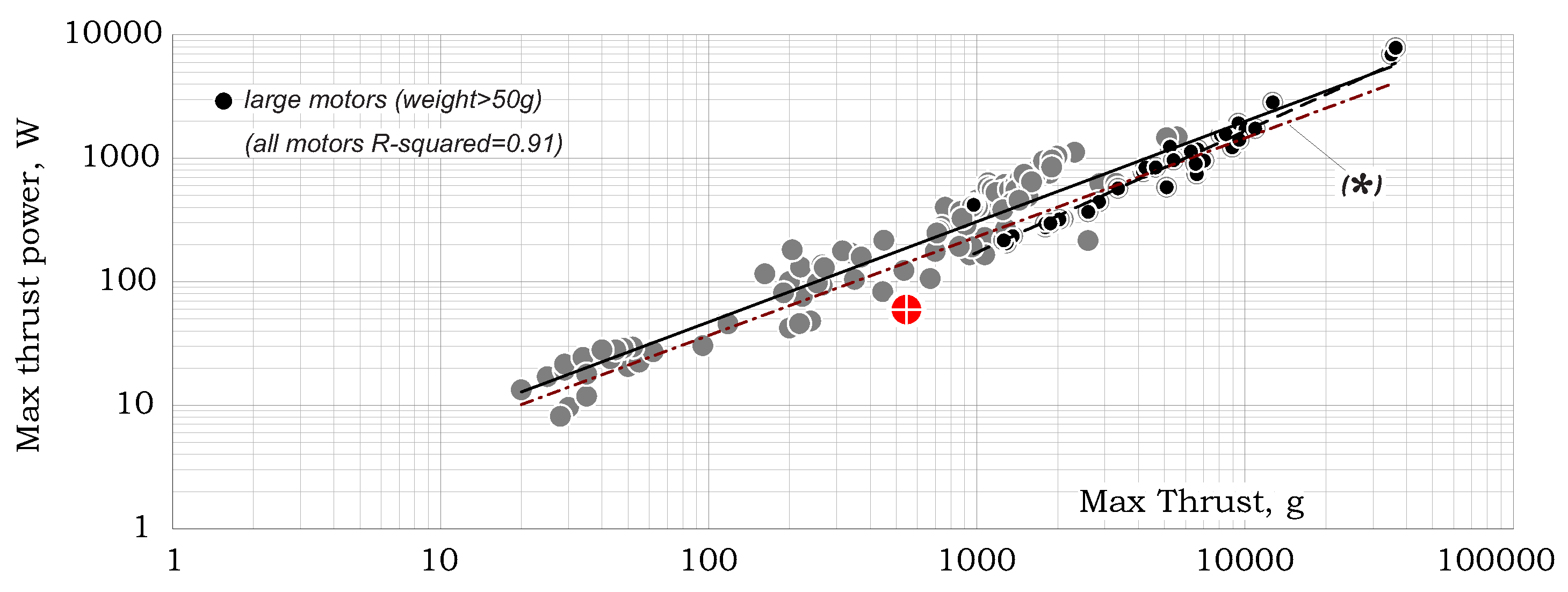
Figure 9 demonstrates a trend-line of the power consumption at max-thrust as a function of max-thrust (single propeller).
Using all data presented, this trend line may be quantified as:
When calculated from the above described voltage and current design trends (Equations (
15) and (
17)), the above equation turns out to be
, which again testifies for the consistency of the presented data.
Note that the above relation is different from the one expected for a constant rotational velocity and constant diameter propeller since, as shown above, for multi-prop vehicles, both rotational velocity and diameters are functions of thrust.
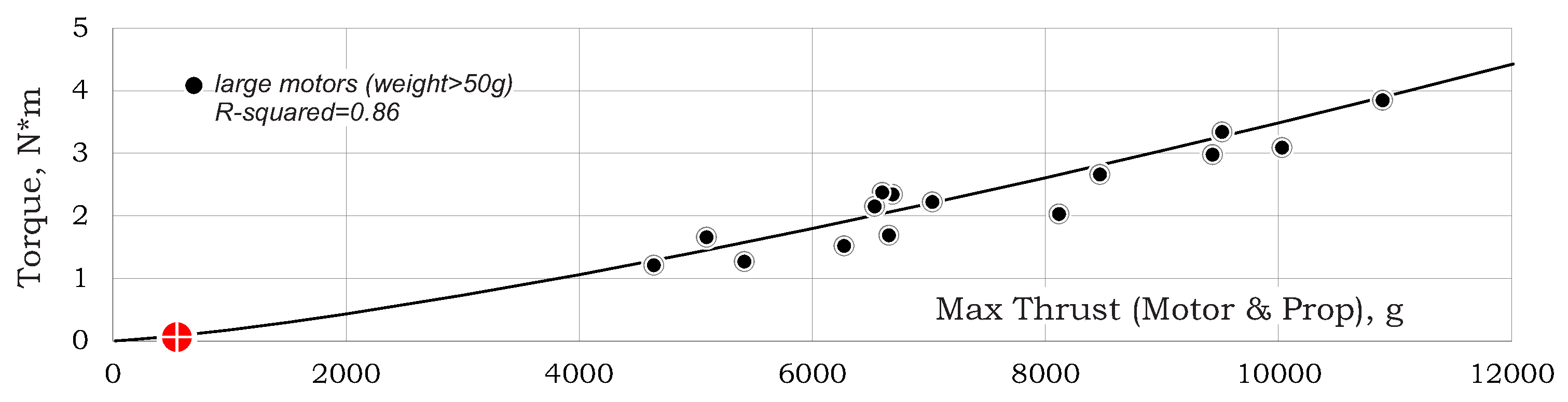
Figure 10 shows the trend-line of torque as functions of thrust.
Note that a relatively small number of data points was found in the open literature and only for relatively large values of max-thrust. This is probably an outcome of measuring challenges for small propellers. The resulting trend-line is given by:
Using Equations (
5) and (
20), one may obtain additional power estimation:
which, as shown by the (*) line in
Figure 9, is similar to Equation (
19) despite the limited available data in
Figure 10.
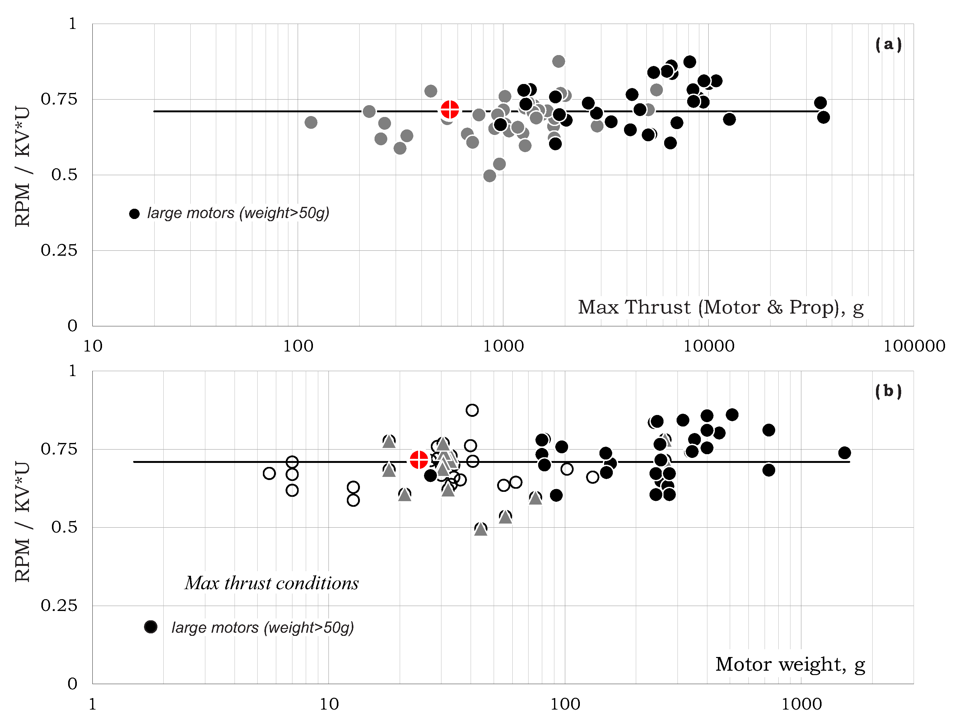
As shown in
Figure 11, the relation between the actual RPM and the RPM without loading (i.e.,
) for all motors is around 0.71. For large motors, the relation is around 0.74. No dependency in max-thrust and/or motor weight was found (note that thrust and weight are linearly related—see Equation (
7)).
Equations (
5), (
13), (
17) also show that the quantity of
does not practically depend on
and equals 0.75.
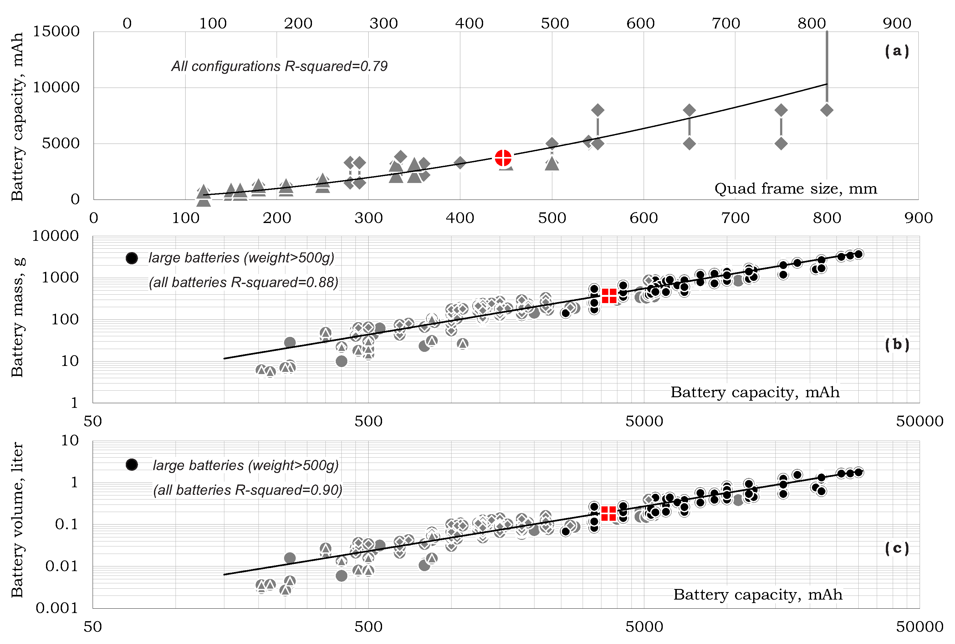
2.5. Design Trend V: Batteries Characteristics
Figure 12a shows a direct relation between battery capacity and the quad frame size that may be expressed as:
Battery mass and volume as functions of battery capacity are presented in
Figure 12b,c as the following relations:
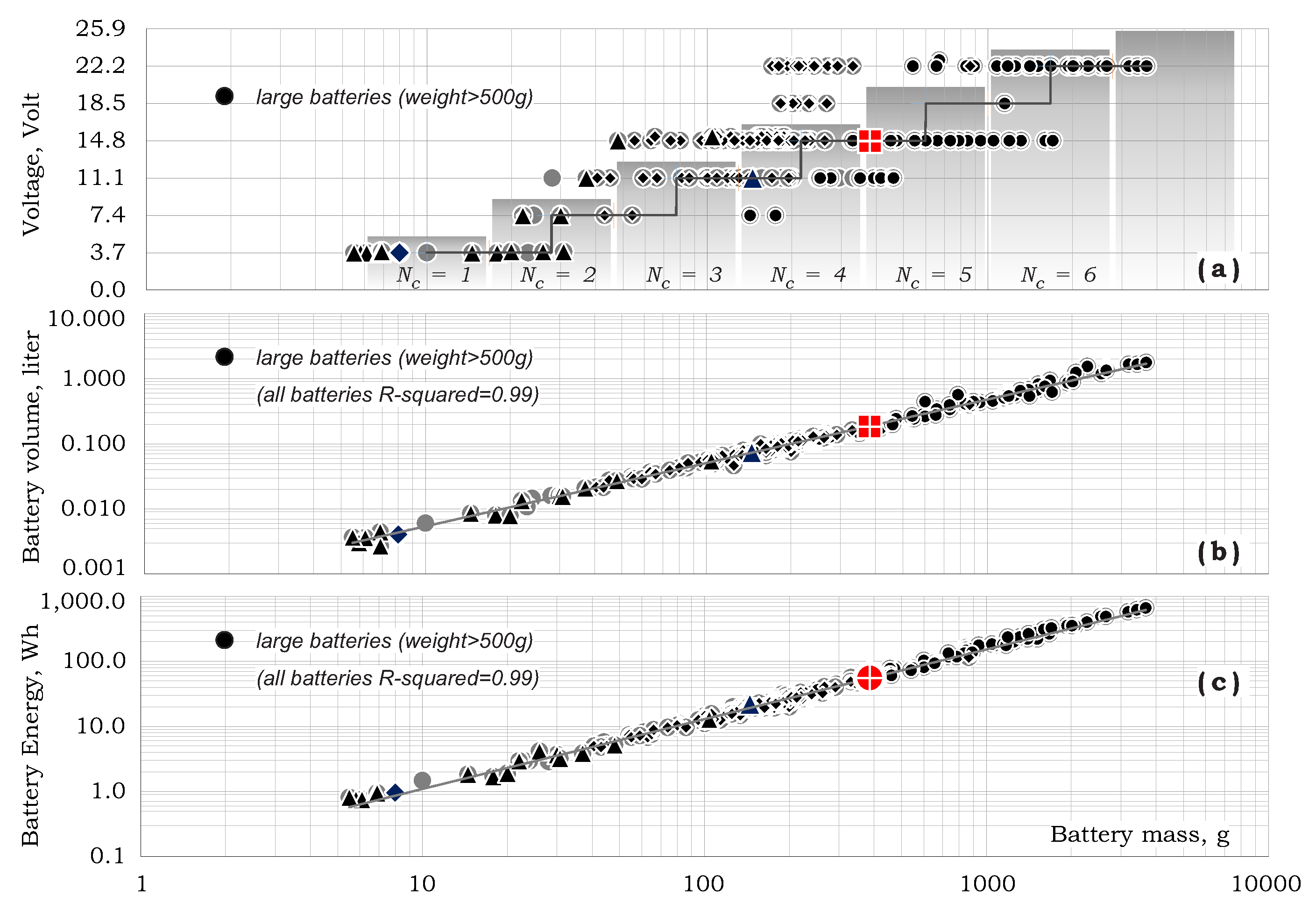
Battery voltage (essentially
Volt where
is the number of 3.7 Volt cells), volume and energy are well correlated with battery mass as shown in
Figure 13.
Figure 13a shows rough relation between the number of cells and battery mass that may be approximated as:
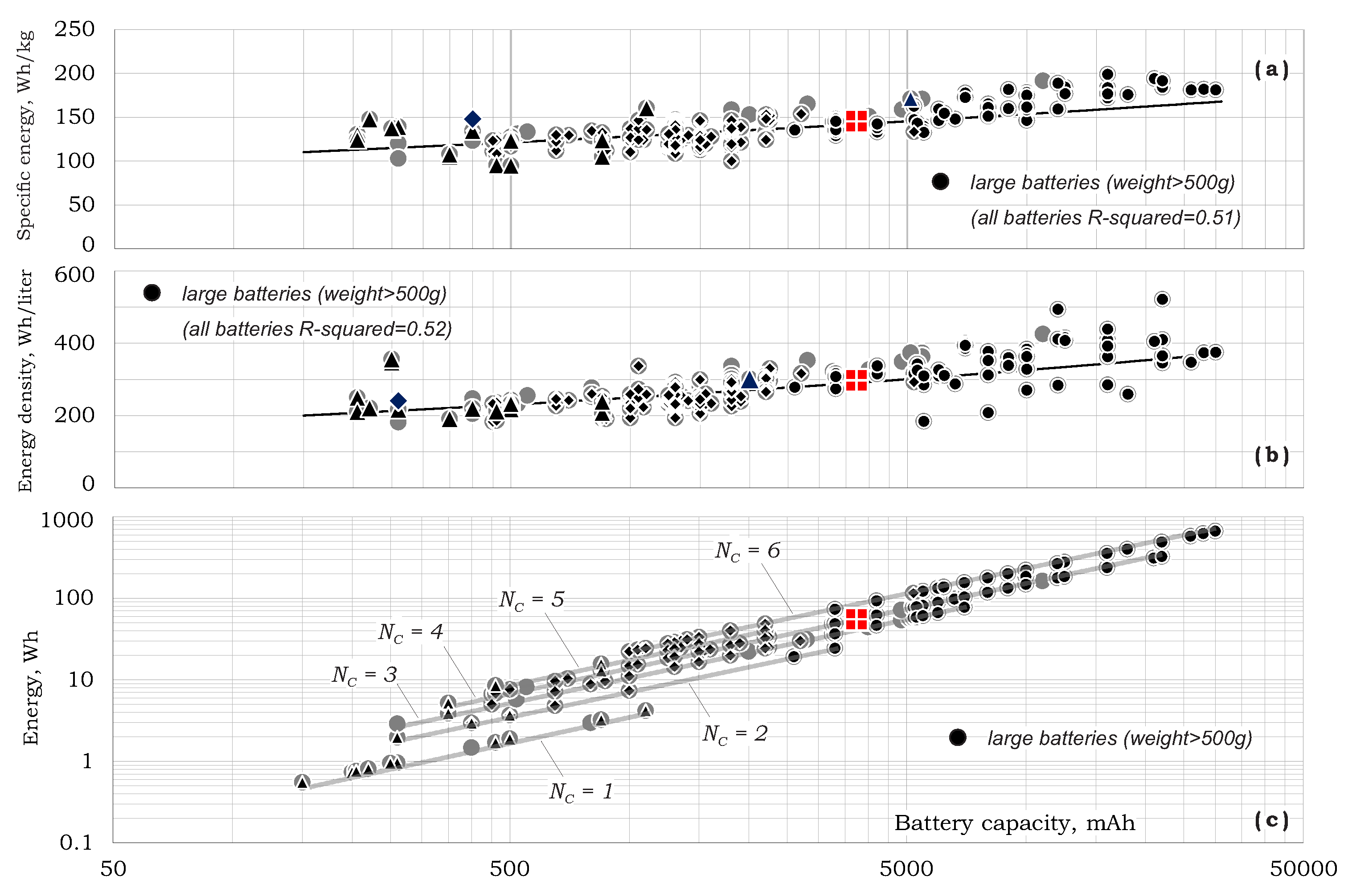
Battery specific energy (
) and battery energy density (
) vs. battery capacity are shown in
Figure 14a,b as:
Note that by definition battery energy is given by:
which corresponds to the lines in
Figure 14c.
2.6. Design Trend VI: Payload
Figure 15 presents trend-lines of the maximum payload vs. gross-weight for full-scale helicopters (FSHs), rotary-wing UAVs (RWUAVs) and some Multi-Prop configurations (MPCs) (the latter were designed by
RAPiD for different payloads and missions by the numerical process described further on).
Payload to gross-weight fraction for the full-scale helicopters and RWUAVs (taken from Refs. [
4,
5]) and the Multi-Prop configurations (of the current study) were found to be:
Note that, in general, compared with full-scale helicopters and Multi-Prop configurations, payload fraction of RWUAVs is lower. A possible explanation for that may be the absence of a clear distinction between payload, equipment, and empty weight, which is included in various sources for RWUAVs.
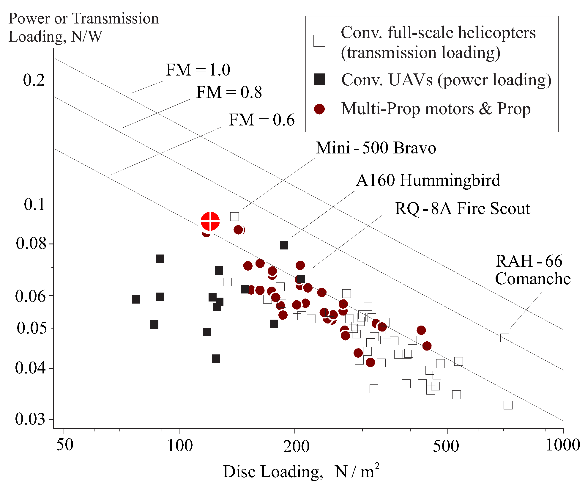
2.7. Design Trend VII: Power Loading vs. Disk Loading
Figure 16 presents power loading vs. disc loading along with lines of constant Figure of Merit (FM). Note that for MPCs, FM is calculated for single propeller and motor combination. As shown, efficiency deteriorates (low FM) for relatively low gross-weights. For larger RWUAVs and MPCs systems, relations between the power- and disc-loading are close to those of full-scale helicopters trend lines.
3. The Design Process
3.1. Local Optimal Mission Analysis
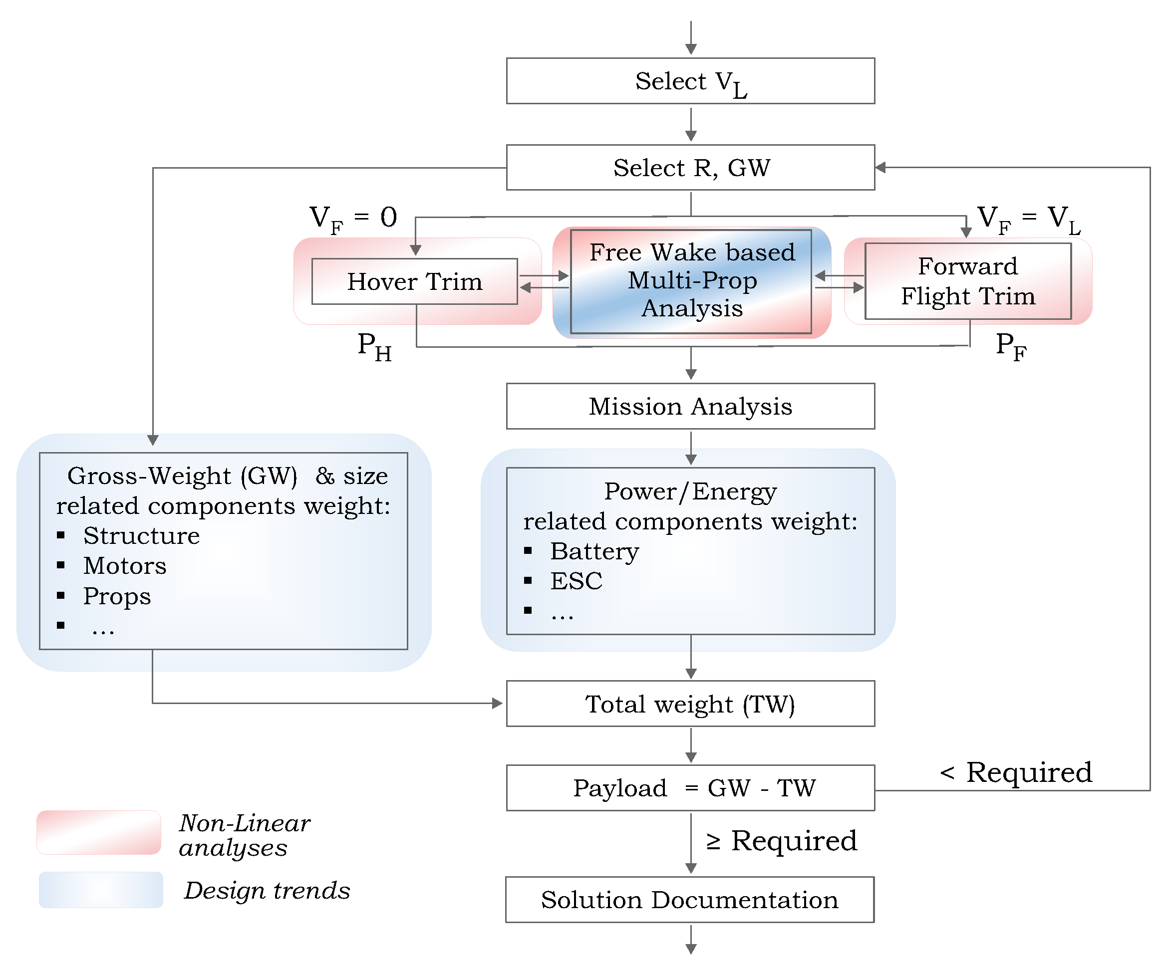
The basic design search process is the one shown in
Figure 17 for a given forward flight velocity. Fundamentally, it is a systematic alternation of the vehicle’s gross weight,
, and the propeller radius,
R. Note that for a given number of propellers of MPCs, the propeller radius determines, almost linearly, the size of the vehicle and mainly the hub-to-hub distance.
This process yields two configurations that are both capable of carrying out the mission: the vehicle of the lowest possible dimension (along with its associated weight) and the vehicle of the lowest possible weight (along with its associated dimension).
As shown in
Figure 17, for any set of values of propeller radius and vehicle gross-weight, nonlinear trim analyses for hover and for a given forward flight velocity (
) is carried out. In this process,
is either the required loiter (forward) flight velocity or a temporary value that will be selected further on.
The above trim procedures exploit a nonlinear multi-propeller analysis. Each trim analysis is essentially a 6DOF nonlinear analysis where the independent unknowns are the propellers’ rotational velocities () and the vehicle roll () and pitch () angles. In cases where the number of propellers is larger than four (), some user pre-defined relations between these parameters are introduced to prevent the need to deal with an under-determined system of equations. Note that the above nonlinear multi-propeller analyses include all hub forces and moments and therefore, take care of the overall torque-balancing of the vehicle as well. The trim analyses make use of RAPiD’s built-in Free-wake/Blade-element scheme with generic (Reynolds and Mach dependent) airfoil polars, in addition to similar polars for the vehicle’s fuselage frame.
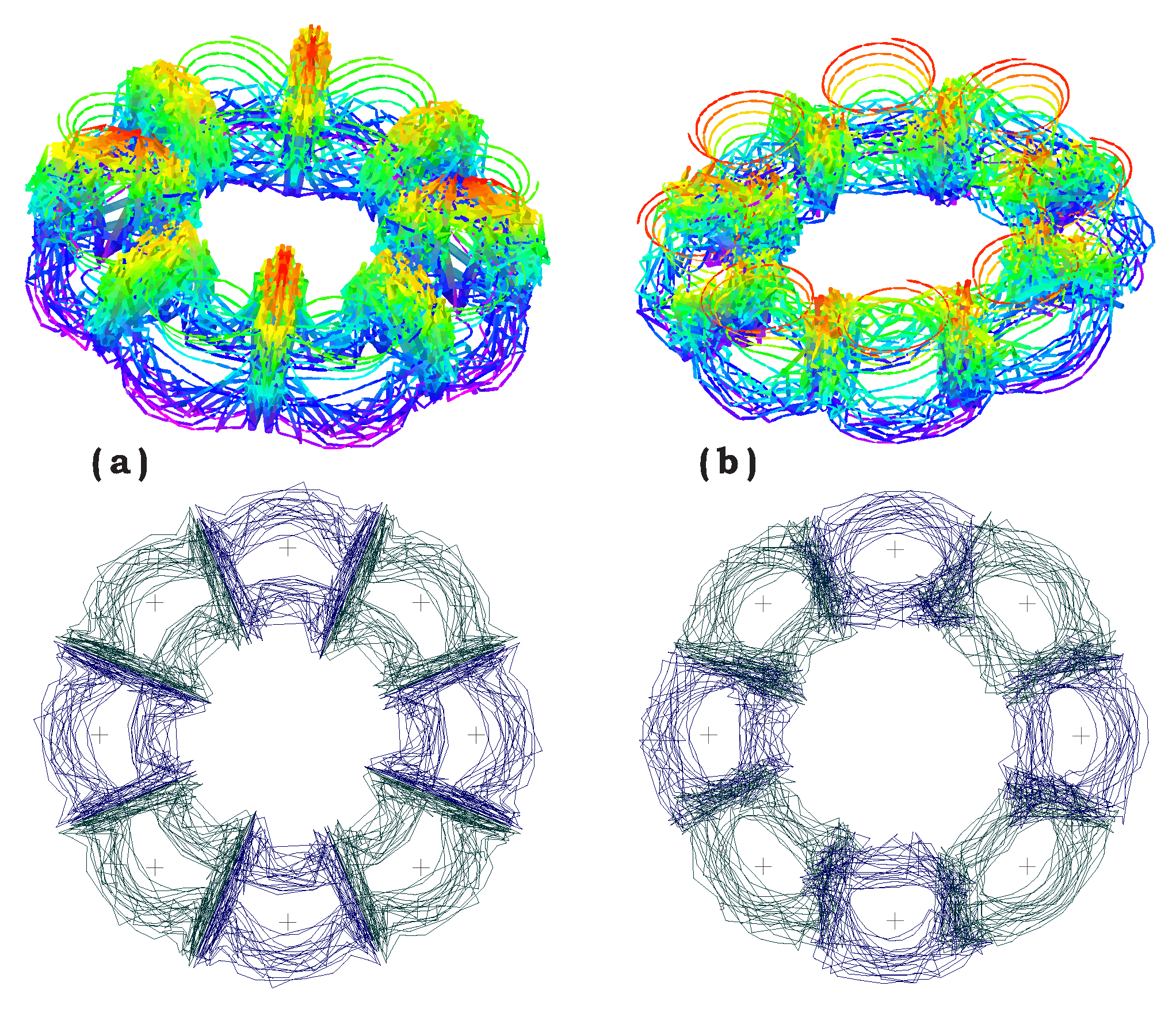
It should also be pointed out that the free-wake multi-propeller analyses allow us to take into account the mutual influence between the propellers’ wake structures. This feature is important for multi-propeller vehicles since, due to the proximity of the propellers, their relative phase angles should also be accounted for.
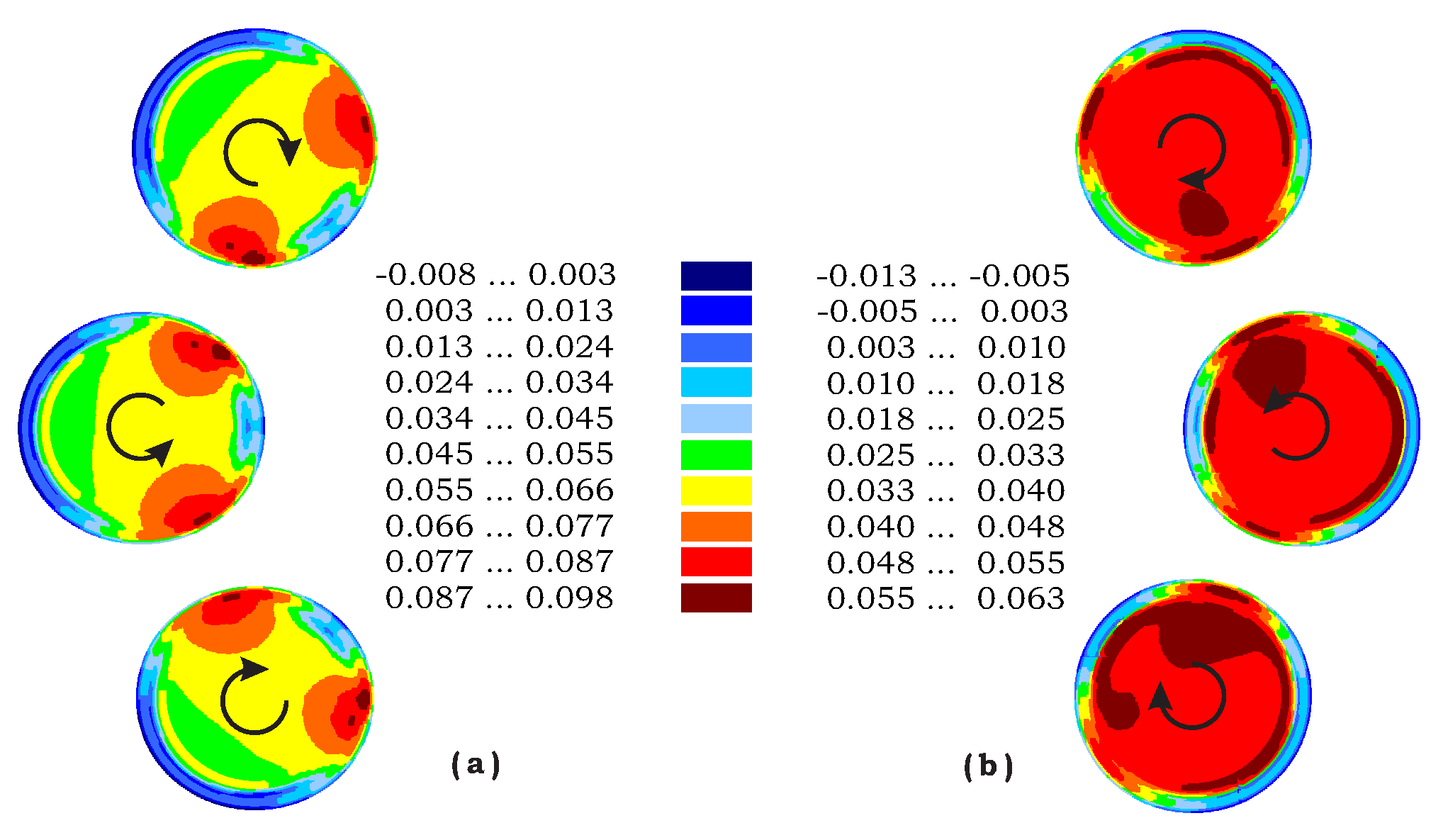
Figure 18 demonstrates 3D and top views of an Octocopter free-wake structures in hover, where the rotational velocities of all propellers are identical. As shown, the wakes’ symmetry of the “in-phase” case (where “the first” blades of each propeller is pointed to the vehicle’s center at the same time) is destroyed in the other “out-of-phase” case. The resulting nondimensional induced velocity distribution over the disc in hover when all propellers are in-phase is shown at the LHS of
Figure 19 while the out-of-phase case is presented at the RHS of
Figure 19 (the propeller phases are random in this example). Obviously, the differences created by the phase angles are important and should be accounted for, as actual achieving a complete “in-phase” rotation is not practical. Note also that the out-of-phase case creates an induced velocity distribution that is more uniform (“smeared”) over most of the disc area.
The outcomes of the trim analyses are the required power in hover and forward flight,
and
, respectively. These values are combined to determine the required total energy:
where
and
are the mission’s hover and forward flight durations, respectively.
Once the power required for both hover and loiter phases and the total energy are known, the weight of all components that depend on , and (e.g., battery weight) are evaluated by the relevant design trends as described in this paper. Parallel to that, the weight of all components that depend on R and (e.g., structural weight) are also evaluated by the above design trends. At this stage, the total vehicle weight (apart from the payload), , may be determined as the sum of all of the above components. This value is used to calculate the remaining weight that may be dedicated to the payload (i.e., ). Once that payload satisfies the required one, the design is completed and valid. Note that the search is initiated by a set of () that consists of relatively small propeller radius and gross-weight values. This set is gradually growing as the search process develops.
To illustrate the above discussion, the following examples will be focused on a quad-rotor configuration.
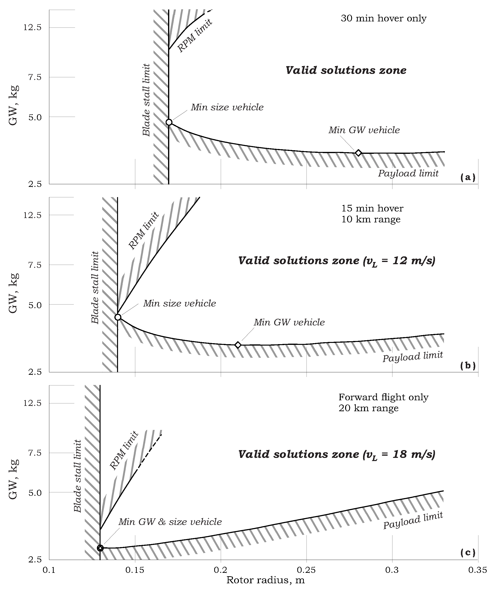
Figure 20 shows typical results of the above-described scheme for the extraction of the vehicle of minimum weight and minimum size for three different missions. Solution zones are confined within the following boundaries: Blade stall limit, RPM limit, and Payload limit. Each point inside these limits represents a valid solution (i.e., a solution that accomplishes the mission with a reserve payload/range/battery/thrust & power levels). The two solutions (the vehicle of minimum weight and the vehicle of minimum size) are clearly marked on the Payload limit. Other points are solutions where heavier or larger vehicles were obtained. For example, as shown in
Figure 20b, for an assumed loiter velocity of 12 m/s, a vehicle of
= 3.3 kg is the lightest one (accompanied by propeller radius
R = 0.21 m) and a vehicle with a propeller of radius of
R = 0.14 m (accompanied by
= 4.4 kg) is the smallest one.
Figure 20c presents the case of a mission that includes forward flight only. As shown, in this case, the points of minimum weight and size collide (
R = 0.13 m,
= 2.825 kg).
3.2. Global Optimal Mission Analysis
As shown above, mission loiter velocity directly influences the vehicle characteristics. Hence, a complete multi-prop optimization is required for any given mission. This process is essentially a search for the optimal combination of the generated vehicle characteristics along with the corresponding loiter velocities. This stage is not required in cases where loiter velocity is dictated by the requirements.
The discussion in what follows is founded on the assumption that a mission is defined in terms of the required payload, the required hover time, and the required range. The design algorithm is then called to determine the best configuration for that mission while the designer has to select between the above-discussed options of a vehicle of the smallest weight or the vehicle of the minimal dimensions. By selecting one of the above two options, the optimal forward flight velocity is determined.
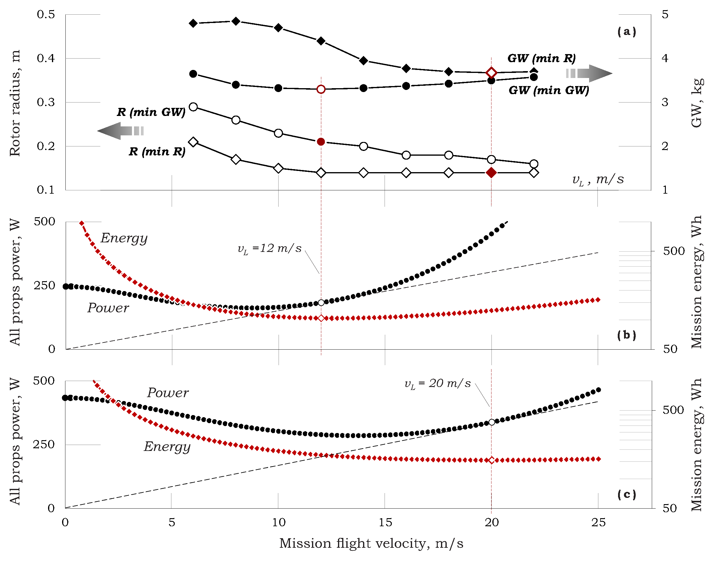
Figure 21 is drawn for a mission of 1.0 kg payload, 15 min hover & 10 km range.
Figure 21a shows four lines that enable the determination of the global “minimum weight” case and the global “minimum radius” case. As shown in
Figure 21a,b, for a “minimum weight vehicle”,
R = 0.21 m,
= 3.3 kg, and one should select a loiter velocity of about 12 m/s, while
Figure 21a,c shows that for a “minimum size vehicle”,
R = 0.14 m,
= 3.675 kg (taken from a very “flat” minimum), and a loiter velocity of 20.0 m/s should be adopted. Note that, in both cases, the loiter velocity is the best velocity for the range of that configuration.
Whenever a specific forward flight velocity is required, the designer has to select between two configurations. For example, in the case under discussion, if forward flight velocity ought to be 16.0 m/s, the algorithm offers a vehicle of R = 0.18 m, = 3.375 kg (as the one of minimal weight) or a vehicle of R = 0.14 m, = 3.775 kg (as the one of minimal radius) while the range between these two bounds is continuously filled with additional designs.
The total mission energy is also presented in
Figure 21b,c. As shown, the vehicle with the minimal weight requires less energy than the vehicle with minimal radius, yet, as indicated above, they both carry the 1.0 kg payload and fulfill the same mission.
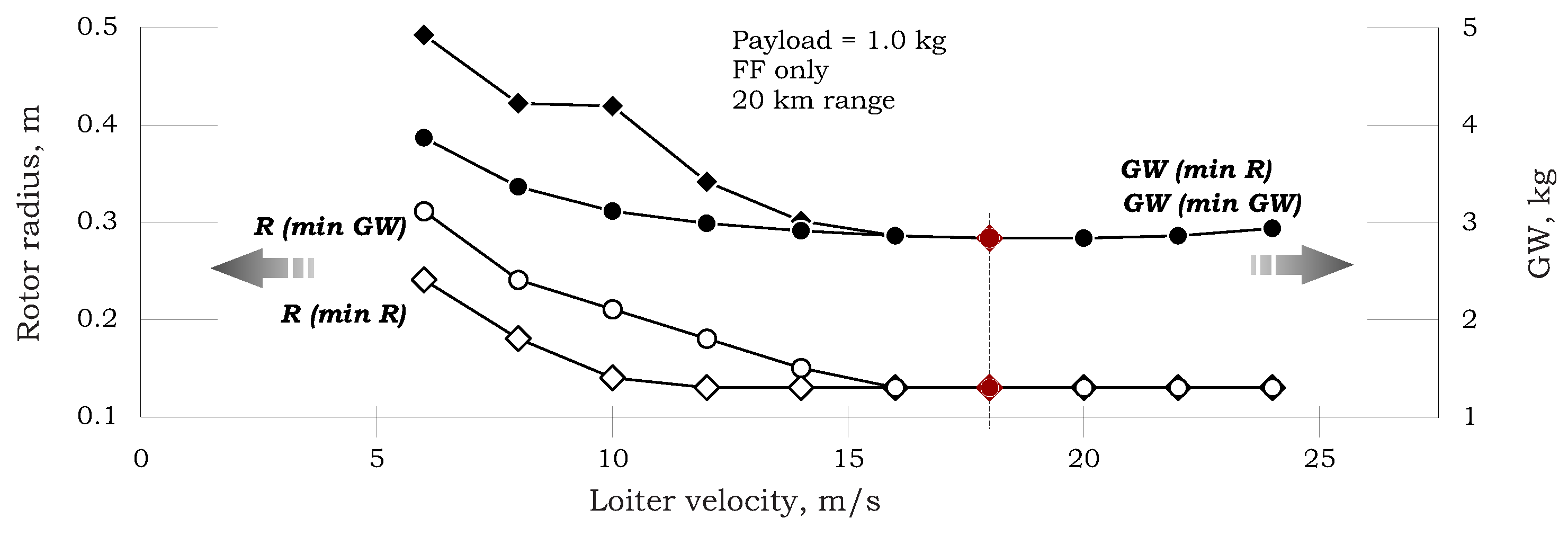
Figure 22 is drawn for a mission of forward flight for a range of 20 km only. As shown for a high enough velocity, both “minimum weight” and “minimum radius” collide (
R = 0.13 m,
= 2.825 kg)—see also
Figure 20c.
4. Conclusions
This paper proposes a mission-oriented preliminary design scheme for Multi-Propeller UAVs that is based on a design trend analysis. The latter is founded on a broad database that was collected from the open literature. The proposed concept is initiated by a pre-assumed mission scenario and yields estimations for geometry parameters, components weight, power, and flight performance. The analysis inherently includes an optimization scheme.
As opposed to first-order and low fidelity analyses that are inevitably used in the first sizing and preliminary stages, this paper offers a design methodology that exposes correlations and design trends in existing flying configurations, and therefore contains many design constraints that emerge only during relatively late stages of the design process.
Unlike full-scale configurations, and with fewer difficulties and costs, Multi-Prop UAVs may be designed to optimally match a variety of missions. The study presented in this paper suggests that tailoring the design for a specific mission may substantially improve range and endurance. Hence, the importance of mission-oriented design is even more obvious and critical for Multi-Propeller UAVs.
Common design trends were found for the most critical design parameters of Multi-Prop UAVs. This phenomenon is reflected by the narrow variations of most of the critical parameters. It leads to the possibility of creating a rough estimation of new designs by trends analysis using minimal computational effort.


