Design of Low Altitude Long Endurance Solar-Powered UAV Using Genetic Algorithm

Abstract

This paper presents a novel framework for the design of a low altitude long endurance solar-powered UAV for multiple-day flight. The genetic algorithm is used to optimize wing airfoil using CST parameterization, along with wing, horizontal and vertical tail geometry. The mass estimation model presented in this paper is based on structural layout, design and available materials used in the fabrication of similar UAVs. This model also caters for additional weight due to the change in wing airfoil. The configuration is optimized for a user-defined static margin, thereby incorporating static stability in the optimization. Longitudinal and lateral control systems are developed for the optimized configuration using the inner–outer loop strategy with an LQR and PID controller, respectively. A six degree-of-freedom nonlinear simulation is performed for the validation of the proposed control scheme. The results of nonlinear simulations are in good agreement with static analysis, validating the complete design process.

1. Introduction

At present, aviation focuses on economic, fuel-efficient, and long-endurance systems that incur low operating costs. The growing demand for airborne operations has resulted in the adoption of unmanned aircraft that can remain in the air for significantly longer times than aircraft with pilots on board. The UAV design has been developed extensively to attain these objectives. At present, UAVs can have an endurance of more than a day [1,2].

Engines that consume fuel are not the solution to the ever-growing demands for airborne time. The endurance of an aircraft must satisfy the mission requirement, which can be a few hours (broadcasting a soccer match), a few days (border patrolling, search and rescue missions), or even years (continuous surveillance, communication relay, and meteorological investigations). Exceptional endurance of months or years is possible with a solar-powered aircraft. Photovoltaic cells mounted on wings can be used to capture solar energy during the daytime. A part of this energy can be used directly to run the propulsion system and onboard electronics, and the remaining part can be stored in onboard batteries for use during the night. If sufficient solar energy can be stored in onboard batteries during the day to last the succeeding night, we can design an aircraft that can fly for years. Theoretically, these solar-powered aircraft can fly forever, and their endurance is limited only by the reliability of the subsystems.

Solar airplanes can be divided into two categories: high altitude long endurance and low altitude long endurance aircraft. Zephyr [3] and Solara [4] are examples of high altitude long endurance solar aircraft. Designed by QinetiQ, Zephyr achieved three world records in July 2010. The UAV was launched for flight trials on 9 July 2010, and stayed aloft for 14 nights (336 h 22 min) at an altitude of 70,740 ft (21,561 m) above the US Army’s Yuma Proving Ground in Arizona. Sky-Sailor [5], Solong [6], and AtlantikSolar [7] are examples of low altitude long endurance solar UAVs. These solar UAVs have demonstrated the potential for perpetual flight and the advantages of solar technology. The present work is also about the design and optimization of fixed-wing low altitude long endurance solar-powered UAVs.

The design process of solar airplanes was not published in the early stages of solar flights [5]. During the past decade, many authors published literature explaining the design process of solar UAVs. However, most of these designs were limited to the theoretical level and did not reach the proof-of-concept phase [8,9,10,11,12,13,14]. Certain designs were manufactured and successfully flown to validate different flight parameters, although these were not tested for a full day–night flight [15,16,17,18,19,20,21]. Very few designs have demonstrated perpetual flight capability [5,6,7].

As far as airfoil selection is concerned, most of the literature compared few airfoils and selected the airfoil with the best lift-to-drag ratio and minimum moment coefficient. The authors in [22] studied 150 airfoils and selected E178 airfoil due to its smooth upper surface. Similarly, [23] discussed MH114, NACA4412, and SD7073 and choose MH114 because of the higher lift-to-drag ratio and large thickness at the trailing edge to facilitate any avionics installation. A similar procedure was adopted in [10,14]. Matter et al. [24] developed an Xfoil-Matlab interface to optimize solar UAV airfoil at a Reynolds number of 2.0 × 10⁵. The optimized airfoil showed an increase of 13% in the lift-to-drag ratio. The authors in [25] also used the genetic algorithm to optimize solar-powered UAV airfoil to maximize the radiation incidence and lift coefficient and minimize the drag by lift ratio. Betancourth et al. [9] selected E212 and the upper surface was considered as a polyline connected by several short line sections. Thereby, it was possible to arrange photovoltaic cells without considerable deformation [26]. In the design of Sky-Sailor [5], W. Engel designed a special airfoil named WE3.55-9.3. The design procedure and objectives were not published. In the proposed framework, the airfoil design is integrated into solar UAV design. Airfoil is also considered a design variable along with wingspan, chord, horizontal and vertical tail span, chord and axial location of the tail assembly. Hence, it is possible to design airfoil considering the overall performance of the UAV. Secondly, if the airfoil changes, rib and wing skin will also change, consequently changing the weight of the UAV. The proposed framework also caters for such changes.

The accurate prediction of the structural mass of a solar UAV is very important. Several mass estimation models are discussed in the literature. A real and simplified airplane structure was dimensioned and actual shear force and bending moment were calculated for the wing and fuselage for the given load case in [11,27]. This method showed deviation from actual data. Noth [5] concluded that models based on the data of HALSOL and twin-boom aircraft [28,29] could not be used for small land-launched solar UAVs. He collected data of over 400 models and sailplanes and ranked solar UAVs in the top 5% in terms of build quality. This model is widely used to predict the structure mass of solar UAVs [10,15,16,19,30,31,32]. As presented in Section 2.3.3, this model also failed to predict the structural mass accurately. The estimation of the structural mass of solar UAVs is significantly influenced by the materials, structural design and layout (double spare, single spare, D-box). In the present study, the UAV dimensions, structural layout, design, and density of materials are used to predict the structural mass. The proposed model is validated with an existing solar UAV with high accuracy.

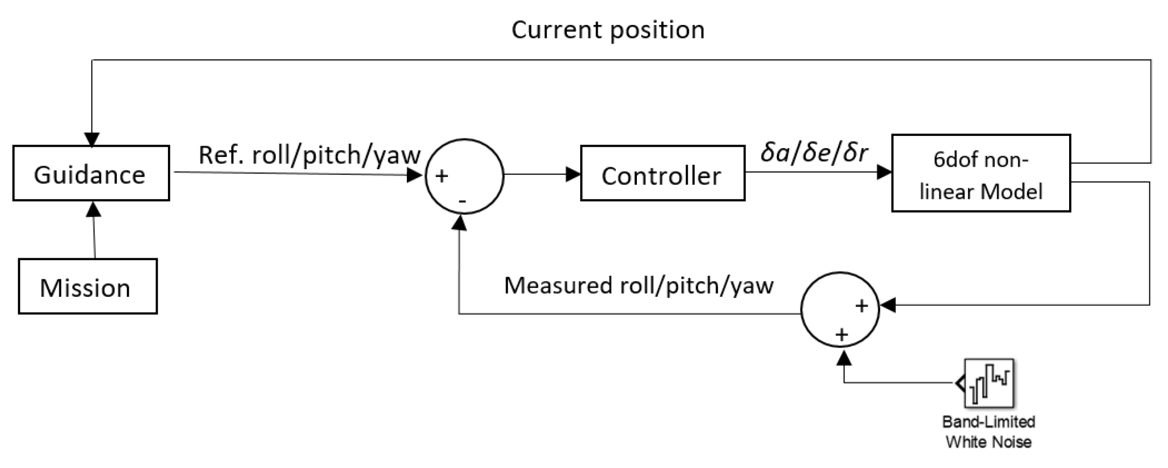
Naturally, the solar UAV configuration must also be stable. Static stability is often measured in terms of the static margin. The literature discussed above provides no guideline about the static margin for solar UAVs. In the proposed framework, the solar UAV is optimized for a user-specified static margin. The optimization is performed for cruise conditions. The Matlab genetic algorithm is used for optimization. Only static stability is incorporated in the optimization framework. To ensure dynamic stability, the dynamic response of the optimized solar-powered UAV is studied. In addition, longitudinal and lateral controls are developed for the optimized configuration. An inner–outer loop control strategy is used with an LQR and PID controller, respectively. Finally, 6-DOF nonlinear simulation is performed in Matlab Simulink to validate the design process and control system.

The remainder of this paper is organized as follows: The design methodology is presented in Section 2, including mass estimation, airfoil parameterization, and stability. The optimization framework is discussed in Section 3. The design of the solar UAV and the optimization results are discussed in Section 4. The dynamic analysis, linear control system design and nonlinear 6-DOF results of the optimized configuration are presented in Section 5. Section 6 presents a few conclusions and discussions, followed by the References section.

2. Design Methodology

2.1. Power Required for Level Flight

During steady level flight, the lift and propeller thrust is equal to the weight and drag, respectively:

$$W=mg=C_L\frac{\rho }{2}S{V}^2$$

(1)

and

$$T=C_D\frac{\rho }{2}S{V}^2$$

(2)

where $W$ is weight, $T$ is thrust, $C_L$ is lift coefficient, $C_D$ is drag coefficient, $S$ is surface area, $V$ is the velocity, $m$ is mass and $g$ is gravitational constant. We can determine the velocity from Equation (1):

$$V=\sqrt{\frac{2mg}{C_L\rho S}}$$

(3)

Using Equations (2) and (3), the power required for level flight, $P_{Level}$, is given by:

$$P_{Level}=TV=\frac{C_D}{C_L^{3/2}}\sqrt{\frac{{\left(mg\right)}^3}{S}}\sqrt{\frac{2}{\rho }}$$

(4)

We replace the surface area in Equation (4) with the aspect ratio, $AR$, to obtain the following equation:

$$P_{level}=\frac{C_D}{C_L^{3/2}}\sqrt{\frac{2AR{g}^3}{\rho }}\frac{m^{3/2}}{b}$$

(5)

2.2. Daily Energy Requirement

The efficiency of the motor ${\eta }_{mot}$, controller ${\eta }_{clrt}$, gearbox ${\eta }_{grb}$, and propeller ${\eta }_{plr}$ must be considered to calculate the power consumption. The power required for the payload $P_{pld}$ and avionics $P_{av}$ is generally known. If the voltage is to be reduced for the payload and avionics, the efficiency of the step-down converter ${\eta }_{bec}$ must also be considered. Therefore, the total power consumption $P_{tot}$ is calculated using the equation given in Noth [5].

$$P_{tot}=\frac{1}{{\eta }_{clrt}{\eta }_{mot}{\eta }_{grb}{\eta }_{plr}}{P}_{Level}+\frac{1}{{\eta }_{bec}}\left(P_{av}+P_{pld}\right)$$

(6)

Considering the efficiency of charging ${\eta }_{chrg}$ and discharging ${\eta }_{dchrg}$ of the batteries, the daily energy consumption $E_{elec tot}$ is given by:

$$E_{elec tot}=P_{tot}\left(T_{day}+\frac{T_{night}}{{\eta }_{chrg}{\eta }_{dchrg}}\right)$$

(7)

where $T_{day}$ and $T_{night}$ are duration of day and night, respectively.

2.3. Mass Prediction Model

It is highly important to accurately estimate the mass of a solar UAV because the power required for level flight is directly proportional to it. The mass prediction model in this study is adopted from Noth [5]. The exception is that rather than estimating the structural mass statistically, a new model based on structural layout, design and available materials is proposed.

2.3.1. Fixed Masses

The fixed mass includes the masses of the payload and avionics. These masses are known and do not vary with the aircraft’s dimensions:

$$m_{fixed}=m_{av}+m_{pld}$$

(8)

where $m_{fixed}$ is fixed mass, $m_{pld}$ is payload mass and $m_{av}$ is avionics mass.

2.3.2. Battery Mass

Depending on the mission requirements, the battery adds significant mass to the system. The battery mass is directly proportional to the product of the power required and the duration of the night and is inversely proportional to its energy density [5].

$$m_{bat}=\frac{T_{night}}{{\eta }_{dchrg}{k}_{bat}}{P}_{tot}$$

(9)

where $m_{bat}$ is battery mass and $k_{bat}$ is energy density of battery.

2.3.3. Structural Mass

The most significant challenge in solar UAV design is the estimation of the structural weight. An overestimation of the weight would result in selecting a heavier battery, which would take a long time to charge and increase the weight. An underestimation of the weight would result in selecting a lighter battery, which would be insufficient to last a night. The weight estimation methods discussed in Section 1 are based on statistical data of different manned sailplanes, unmanned radio-controlled models, NASA high-altitude prototypes, and twin-boom configurations. These models are derived from their geometric parameters such as wing area, wing aspect ratio and wingspan, rather than the structural layout, design and materials used. The structural weights of the four solar UAVs estimated using different models are presented in

Table 1. Comparison of structural weight estimation models.

UAV	b (m)	AR	Weight in kg
			Noth [5]	Stender [28]	Rizzo [29]	Leutenegger [11]	Actual
Sky-Sailor	3.2	12.9	0.87	2.466	7.04	0.51	0.748
SunSailor	4.2	13.15	2.016	3.743	10.056	0.85	1.70
AltantikSolar	5.69	18.7	4.733	5.381	14.95	-	1.52
Zephyr	18	11.6	189.43	37.461	67.91	51.0	20.0

. It is important to mention here that, for solar UAV design studies discussed in the preceding section, structural weight was quoted for very few prototypes.

The most common wing structural layouts are double circular spare [16], single circular spare [7,18] and D-box [5,20,21]. Even for a specific structural layout, there can be many variations in the numbers of ribs, stringers, the diameter and thickness of spares and the thickness of ribs and skin. However, for a given span and aspect ratio, with different structural layouts, any mass prediction models presented in Table 1 will give the same prediction. In the proposed design process, weight estimation is based on the specific structural design, layout, respective dimensions and actual material used in the fabrication of solar UAVs.

The wing structural layout selected for the current study is double circular spares with ribs and stringers. The reasons for this selection are the simplicity and practical experience in fabricating this layout. The selection of the material is also very important for solar UAV design. The materials should be lightweight but adequately strong enough to withstand flight loads. For the current study, the materials considered are 3 k carbon fiber, light density balsa wood and plywood. Several prototypes such as MARAAL [16], Sky-Sailor [5], AtlantikSolar [7], SunSailor [33] and LEEUAV [20] also used carbon fiber and balsa wood as primary materials.

There is no study conducted for structure design. The structure design is adopted from a reference UAV available at the UAV design lab, Beihang University, Beijing. The reference UAV is also a solar-powered UAV with a total weight of 7.5 kg. This UAV has been extensively tested in various experimental flights with a cruise speed up to 15 m/s. The reference UAV has a front and rear spare with a thickness of 1 mm and diameter of 20 mm and 12 mm, respectively. Ribs are made from balsa wood with a thickness of 2 mm. Four stringers run along the span. The stringer at the trailing edge is made from balsa wood. The other three stringers are made from plywood. Wing surface is also balsa wood of 1 mm thickness. The reference UAV also has a third shorter spare adjacent to the front spare. The purpose of this spare is to provide extra stiffness and install batteries if required. The horizontal and vertical tail design is similar to the wing, except they have only one spare with a thickness and diameter of 1 mm and 12 mm, respectively. The tail boom is also a carbon fiber tube with a thickness and diameter of 1 mm and 20 mm, respectively. The fuselage is made from a carbon fiber sheet of 1 mm thickness. To estimate the length of the fuselage, similar solar UAVs are studied (

Table 2. Ratio of fuselage length to wingspan.

Solar UAV	Wingspan (m)	L. Fuselage (m)	Ratio
Sky-Sailor [5]	3.2	0.82	0.256
AtlantikSolar [7]	5.7	0.81	0.142
SunSailor [33]	4.2	0.94	0.224
		average	0.207

). From the literature discussed in Section 1, the fuselage length of only three prototypes was quoted. From the geometric data of these three prototypes, it is concluded that the fuselage length could be assumed to be 21% of the wingspan.

The fuselage mass is determined based on its length and the average diameter of the reference solar UAV. A heat sink plastic film is used for the wing and tail surfaces in conjunction with balsa wood to save weight. The user can input the percentage coverage of balsa wood (100% implies that the entire wing and tail surface would be of balsa wood, i.e., plastic film would not be used).

The shape of the rib is identical to that of the airfoil and varies as the airfoil undergoes modifications during the optimization process. The user can change the number of holes and their respective locations. The diameters of these holes are input as percentages of the airfoil thickness at the respective locations. This prevents misleading results when the input diameter value is larger than the airfoil thickness at that particular location. The wing airfoil of the reference UAV is NACA 6409, and its tail airfoil is NACA 0009.

The reference UAV is disassembled for measurements. Mass is calculated using geometric dimension, structural layout, design and material densities. Material densities considered for carbon fiber, balsa wood and plywood are 1600 kg/m³, 90 kg/m³ and 260 kg/m³, respectively. The structural components of the reference UAV are shown in Figure 1.

The calculated and actual masses are compared in

Table 3. Comparison of calculated and actual structural mass.

Component		Parameter	Value	Actual Mass (kg)	Estimated Mass (kg)
Wing		Span	5.7 m	1.32	1.36
		Chord	0.3 m
	Front Spare	Thickness	0.001 m
		Radius	0.01 m
	Middle Spare	Thickness	0.001 m
		Radius	0.01 m
		Length	0.9 m
	Rear Spare	Thickness	0.001 m
		Radius	0.006 m
	No of ribs	Ribs/Unit Span = 9	51
	Balsa Coverage	Upper Wing	100%
		Lower Wing	30%
Tail	H. Tail	Span	1 m	0.17	0.163
		Chord	0.22 m
	V. Tail	Height	0.4 m
		Chord	0.25 m
	Tail Spare	Thickness	0.001 m
		Radius	0.006 m
	Balsa Coverage		50%
Tail Boom		Length	0.73 m	0.068	0.0735
		Thickness	0.001 m
		Radius	0.01 m
Fuselage		Thickness	0.001 m	0.388	0.391
		Length	1.2 m
		Diameter	0.065 m
Total				1.946	1.9875

. The total estimated mass of the wing also contains the mass of stringers.

The individual components and total structural mass of the reference UAV and the calculated mass are very close. The advantage of using this type of method is that we can accurately predict the mass given the available materials, structural layout and design. This method is very flexible and can be extended to D-box structural layout. The design of the wing and tail ribs is shown in Figure 2. The modeled airfoils exactly replicate the actual airfoils.

2.3.4. Solar Cells Mass

To estimate the mass of the solar cell, the required solar cell area is computed using the following equation:

$$A_{sc}=\frac{\pi }{2{\eta }_{sc}{\eta }_{cbr}{\eta }_{mppt}{\eta }_{wthr}{I}_{max}}\left(1+\frac{T_{night}}{T_{day}}\frac{1}{{\eta }_{chrg}{\eta }_{dchrg}}\right)P_{tot}$$

(10)

where $A_{sc}$ is the area of the solar cells, ${\eta }_{sc}$ is the efficiency of the solar cells, ${\eta }_{cbr}$ is the efficiency of the camber, ${\eta }_{mppt}$ is the efficiency of the Maximum Power Point Tracker (MPPT), ${\eta }_{wthr}$ is the margin factor for clouds and $I_{max}$ is the maximum irradiation. The mass of the solar cells can be calculated by considering the encapsulation and mass density of the solar cell.

$$m_{sc}=A_{sc}\left(k_{sc}+k_{enc}\right)$$

(11)

where $m_{sc}$ is the mass of solar cells, and $k_{sc}$ and $k_{enc}$ are solar cells and encapsulation mass density, respectively.

2.3.5. Maximum Power Point Tracker Mass

To extract the maximum power from the solar cell, we must track the optimal working point on its current-to-voltage curve using MPPT. This point shifts continuously because of the irradiance conditions. The mass of the MPPT is calculated using:

$$m_{mppt}=k_{mppt}{I}_{max}{\eta }_{sc}{\eta }_{cbr}{\eta }_{mppt}{A}_{sc}$$

(12)

where $m_{mppt}$ is the mass of MPPT and $k_{mppt}$ is the mass-to-power ratio of MPPT.

2.3.6. Propulsion System Mass

The propulsion system consists of an electric motor, controller, electronics, gearbox, and propeller. Based on the statistical analysis from Noth [5], the mass of the entire propulsion system is given by:

$$m_{prop}=k_{prop}{P}_{level}$$

(13)

where $m_{prop}$ and $k_{prop}$ are the mass and mass-to-power ratio of the propulsion system, respectively.

2.4. Stability

Stability is generally defined as the capability of an aircraft to return to its equilibrium state after any imbalance, gust, and control input. There are two types of stability: static and dynamic. For an airplane to be statically stable, the sign of the ${\mathrm{C}}_M{}_{\alpha }$ curve must be negative. A statically stable plane tends to return to its equilibrium position. A statically unstable plane continues to increase the orientation after disturbance. Meanwhile, a statically neutral plane regains its position, implying that the net force or moment acting on the aircraft in the new orientation is zero. Static stability is generally measured in terms of the static margin, which is defined as follows:

$$SM=\frac{X_{NP}-X_{CG}}{L_{ref}}\times 100\%$$

(14)

$L_{ref}$ is the reference length, $X_{CG}$ is the center of gravity and $X_{NP}$ is the neutral point. In the proposed framework, the solar UAV is optimized for a user-specified static margin at the equilibrium position. As the geometry of the UAV is changed during optimization, the neutral point will also change. One methodology is to fix $X_{CG}$ and calculate the static margin using $X_{NP}$ and $L_{ref}$. In this case, an additional constraint is required to fulfill the static margin requirement. In the current study, the required $X_{CG}$ is calculated using $X_{NP}$, $L_{ref}$ and the static margin. The aerodynamic moment is then shifted to the required $X_{CG}$ for analysis. For the design of a solar-powered UAV, a static margin of 15% is selected.

2.5. Airfoil Parameterization

The airfoil must be parameterized to modify it during optimization. Several methods for airfoil parameterization are available in the literature (Hicks–Henne bump function [34], CST (class function/shape function transformation) [35], and PARSEC [36]). In the present study, CST is used for airfoil parametrization. This method can define a wide range of airfoils and can be extended to other shapes such as squares and circles. It is defined as:

$$Z_{upper}=C_{N2}^{N1}\left(x\right)·S_{upper}\left(x\right)+x·\mathsf{\Delta }{Z}_{upper}$$

(15)

$$Z_{lower}=C_{N2}^{N1}\left(x\right)·S_{lower}\left(x\right)+x·\mathsf{\Delta }{Z}_{lower}$$

(16)

The class function $C_{N2}^{N1}\left(x\right)$ is defined as:

$$C_{N2}^{N1}\left(x\right)=x^{N1}·{\left(1-x\right)}^{N2}$$

(17)

where $\mathsf{\Delta }Z$ defines the trailing edge thickness and $x\in \left[0,1\right]$. For airfoil shapes, $N1=0.5$ and $N2=1$. $S\left(x\right)$ is defined as a linear combination of Bernstein polynomials and is given by:

$$S\left(x\right)={\displaystyle \sum _{i=0}^n}{a}_i{b}_{i,n}\left(x\right)$$

(18)

where

$$b_{i,n}\left(x\right)=\left(\begin{array}{c}n\\ i\end{array}\right)x^i{\left(1-x\right)}^{n-i}$$

(19)

$a_i$ is the Bernstein coefficient and $n$ is the degree of the polynomial. The quality of the CST airfoil is significantly dependent on the degree of the polynomial. In Figure 3, CST airfoils for polynomials of order zero, two, and four for NACA 63–137 are plotted in conjunction with the original airfoil. It is evident that the polynomial of order four provides a very good representation of the original airfoil. Hence, a fourth-order polynomial is used in the present optimization framework. It provides ten airfoil parameters: five each for the lower and upper portions.

3. Optimization Framework

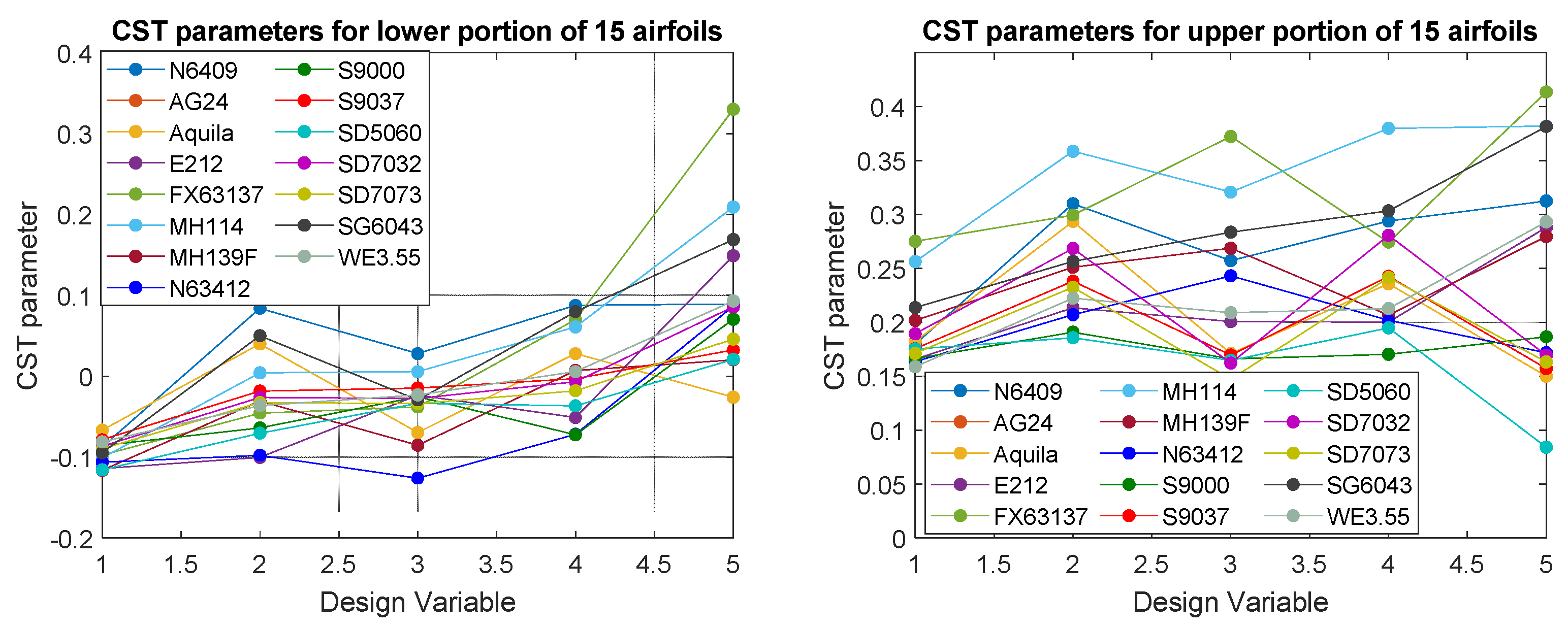
The optimization framework is modeled in Matlab using the genetic algorithm (GA) with selection, mutation and crossover functions. Seventeen design variables are considered. The first 10 design variables are the CST parameters for the airfoil. The lower and upper bounds for the airfoils are based on 15 airfoils recommended for the design of solar UAVs in different publications. These airfoils are parameterized using CST. For each parameter, the highest and lowest of the values of all the airfoils are used as the upper and lower bounds, respectively (Figure 4).

This results in very wide design space and the possibility of the production of non-feasible and unsmooth airfoils. The airfoils produced during optimization are passed through a series of assessments (maximum thickness, camber, curvature of the lower portion, and quality of the trailing edge) to ensure a feasible and smooth airfoil. The details of the design variables are listed in

Table 4. Design variables of solar UAV.

Design Variables	Description	Bounds
1–10	CST parameters of airfoil	Figure 4
11	Wingspan	5.0–6.0 m
12	Wing chord	0.275–0.31 m
13	Axial location of tail (Origin at wing airfoil leading edge)	1.3–1.5 m
14	Horizontal tail chord	0.2–0.31 m
15	Vertical tail chord	0.2–0.3 m
16	Horizontal tail span	0.9–1.1 m
17	Vertical tail height	0.4–0.5 m

. There is no geometric and aerodynamic twist in the wing. The wing planform is a rectangle without taper and sweep. The dihedral angle of 7° is used from 45% of the wing semi-span for this study. The tail is a simple T-shape design with the horizontal tail mounted at the top of the vertical tail. The fuselage is not considered in the optimization, as recommended by the developer of Xflr5 (Xflr5 GUI). However, the fuselage and tail boom’s skin friction drag and form drag are considered in the optimization and calculated using W.H. Mason’s FRICTman code [37].

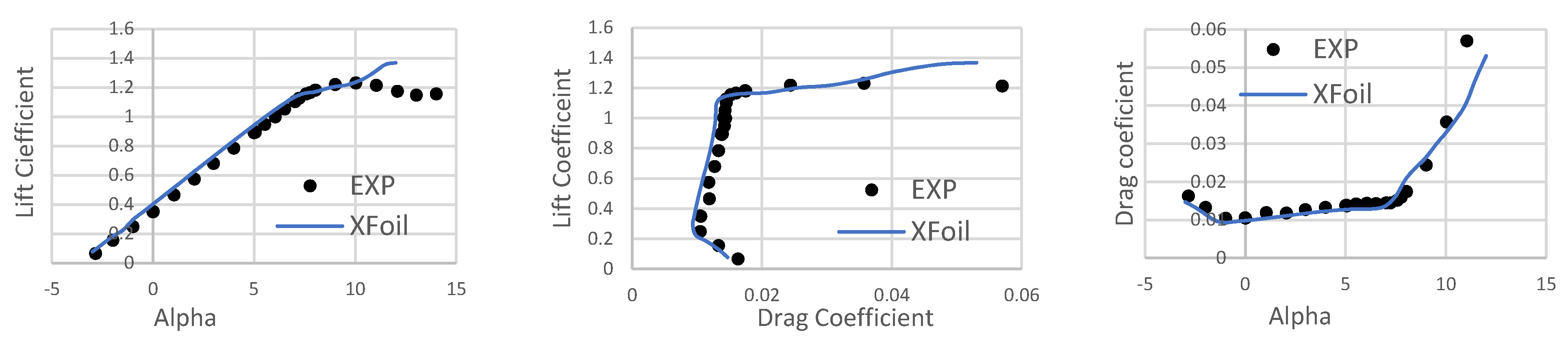
During optimization, Xflr5 is used to obtain aerodynamic coefficients. Xflr5 is an analysis tool for airfoils based on Xfoil’s airfoil analysis and also includes wing design and analysis capabilities using the lifting line theory, vortex lattice method and 3D panel model. The validation of Xfoil with experimental data of E387 airfoil at Reynolds number 2.0 × 10⁵ is shown in Figure 5. The results are in good agreement in the linear region. As solar UAVs fly at a lower angle of attack, Xflr5 is a good choice for preliminary design.

The analysis is performed in the following sequence:

• Matlab GA provides 17 design variables.
• The first 10 variables are used for airfoil generation using CST. The quality of the CST airfoil is assessed. When the airfoil is not smooth, the iteration is terminated, the objective function is assigned a value of 200, and the next set of design variables is considered. When the airfoil is smooth, we proceed to Step 3.
• The CST airfoil and other geometry parameters are used to perform aerodynamic analysis in Xflr5. A VB script is written that calls the Xflr5.exe, writes all the variables in the respective fields, performs analysis, and writes the output file.
• Matlab reads the Xflr5 output file. This file contains all the aerodynamic forces and moment coefficients. The pitching moment coefficient is transferred to the required C.G. location calculated from the static and neutral points using Equation (14).
• The trim (zero pitching moment) angle of attack and the corresponding lift and drag coefficients are calculated.
• The structural mass of the solar UAV is calculated (Section 2.3.3).
• The total mass is calculated by solving a cubic equation as presented in [5].
• Equations (1), (6) and (9)–(13). If the required solar cell area is greater than the wing area, the iteration is terminated, the objective function is assigned a value of 200, and the next set of design variables is considered.
• If the required solar cell area is less than the wing area, the objective function is calculated as follows:

  $$Obj=abs\left(Lift-Weight\right)+P_{tot}$$

  (20)

The first term ensures that the lift produced is equal to the weight, whereas the second term helps to decrease mass and increase $C_L^{3/2}/C_D$. The number of generations is set to 100 with a population size of 25.

4. Design of Solar UAV

The solar UAV is designed to fly over a specific location on a specific day of the year. Given these specifications, $t_{night}$ and $t_{day }$ are retrieved. The designed UAV is oriented to fly for $t_{night}$ hours. The next step is to add robustness to the design [7].

The first consideration is to have multiple-day endurance, $t_{exc}^{Date}$. This implies a window of a specific number of days or months for flight operation. To achieve this, the additional night duration, owing to date change, must be considered:

$$t_{exc}^{Date}=t_{night}^{max}-t_{night}^{min}$$

(21)

Meteorological factors such as clouds and water fog in the early morning and evening, $t_{exc}^{Weather}$, and aggressive flight conditions during the night,$t_{exc}^{Plevel}$, such as gusts, may result in additional power consumption. The total demand surplus time is:

$$t_{exc}^{req}=SUM\left(t_{exc}^{Date}+t_{exc}^{Weather}+t_{exc}^{Plevel}\right)$$

(22)

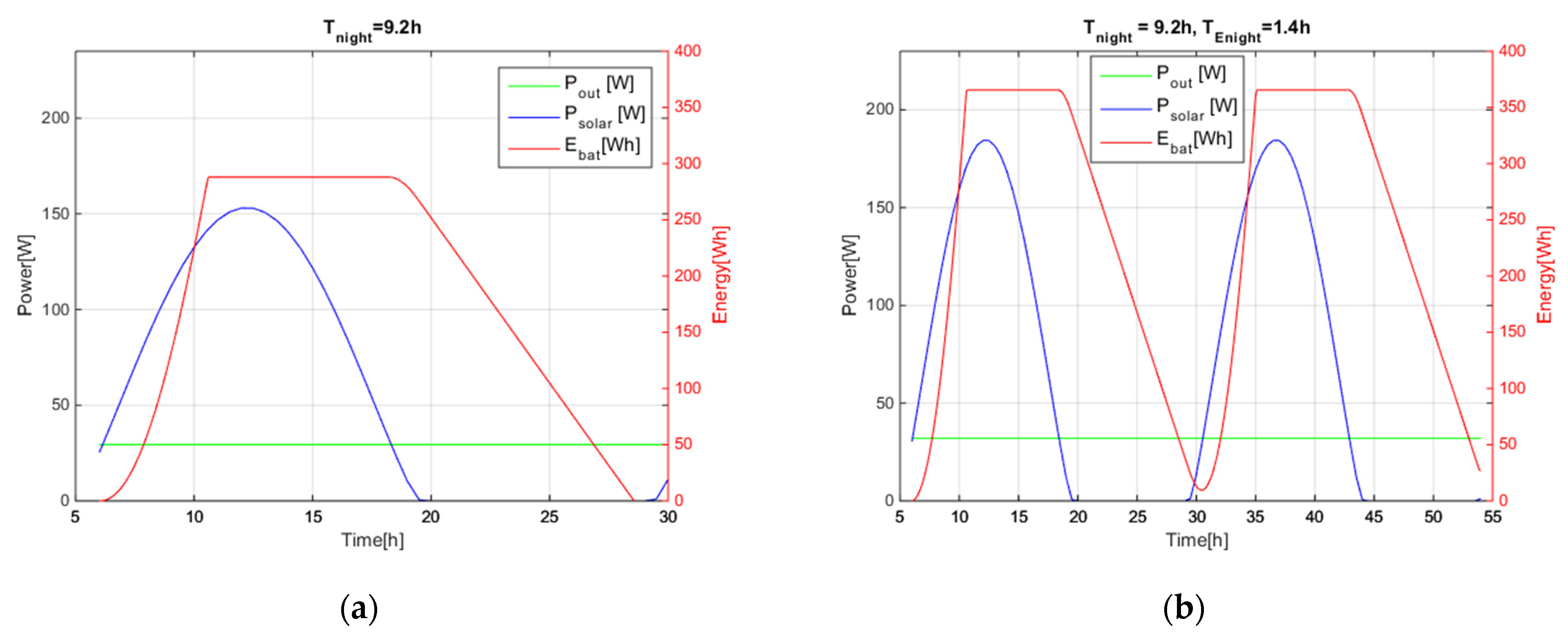
This design is not fully robust. This is because the energy stored in the batteries starts to drain when the available solar power is less than the power required for level flight, which can occur more than 1 h before sunset. To illustrate this, a solar UAV is designed to perform a full-night operation in Beijing or Tianjin (40° N). The optimum time to perform a full night operation is 21 June, when $t_{day}=14.8$ h and $t_{night}=9.2$ h. In this design (referred to as Design-1), $t_{exc}^{req}$ = zero. This implies that we assume ideal conditions during flight. The input parameters for the design process are listed in

Table 5. Input parameters for solar UAV design.

Inputs	Description	Value
$g$	Gravitational constant	9.81 m/s2
$Alt$	Altitude	700 m
$rho$	Density	1.15 kg/m3
$V_{cruise}$	Cruise velocity	8.5 m/s
$S.M.$	Static margin	15%
${\eta }_{mctrl}$	Efficiency of motor control	0.9
${\eta }_{motor}$	Efficiency of motor	0.85
${\eta }_{grbox}$	Efficiency of gearbox	0.97
${\eta }_{prop}$	Efficiency of propeller	0.80
$m_{avi}$	Mass of avionic	0.5 kg
$m_{pld}$	Mass of payload	0.1 kg
$P_{avi}$	Power for avionics	5 W
$P_{pld}$	Power for payload	0.5 W
$k_{sc}$	Mass density of solar cells	0.33 kg/m2
$k_{enc}$	Mass density of encapsulation	0.26 kg/m2
${\eta }_{sc}$	Efficiency of solar cells	0.19
$k_{prop}$	Mass-to-power ratio	0.008
${\eta }_{MPPT}$	Efficiency of MPPT	0.95
${\eta }_{chrg}$	Efficiency of charging	0.95
${\eta }_{dchrg}$	Efficiency of discharging	0.95
$k_{bat}$	Energy density of battery	240 Wh/kg

.

The energy simulation for Design-1 is shown in Figure 6a. It is evident that although the battery is designed for $t_{night}=9.2\mathrm{h}$, it is insufficient for a continuous 24 h flight and is drained completely before sunrise. This is because the battery starts to supply the energy when the available solar power is less than the power required to maintain level flight. In this case, it is approximately 1.4 h earlier than sunset. In the next design (referred to as Design-2), an additional time of 1.4 h (denoted as $t_{Enight}$) is included. The energy simulation for Design-2 is presented in Figure 6b. This design demonstrates the capability for continuous 24 h flight. The battery shows a minimum capacity of 10.8 Wh at sunrise, which corresponds to less than half an hour of flight. Although Design-2 displays potential, it is an ideal design. To add robustness, Equation (22) is incorporated (referred to as Design-3). The associated parameters are as follows:

$$t_{Enight}=1.4 \mathrm{h},t_{exc}^{clouds}=k_{ccf}\times t_{night}^{max},t_{exc}^{Plevel}=2.4\mathrm{h},t_{exc}^{date}=t_{night}^{max}-t_{night}^{min}$$

$k_{ccf}$ is the cloud or fog thickness factor [38] and is considered to be 0.2.

For a solar UAV that can perform multi-day operation during a three month window (1 May to 30 July), $t_{night}^{max}=10.3 \mathrm{h}$, $t_{night}^{min}=9.2 \mathrm{h}$, and $t_{exc}^{date}=1.1 \mathrm{h}$. Hence, for Design-3, $t_{exc}^{req}=5.56 \mathrm{h}$. The total required time of flight for batteries is given by:

$$t_{tot}^{req}=t_{night}^{min}+t_{Enight}+t_{exc}^{req}$$

(23)

An important parameter of a battery is the state of charge, SOC. It is defined as the current battery capacity to the rated battery capacity. The over-discharging of a battery can attenuate its usable capacity. In addition, the minimum SOC may be limited to 5–10% to increase the battery life cycle [39]. A minimum SOC of 10% is imposed in Design-3. The output parameters for these three designs are listed in

Table 6. Output parameters.

Output	Design-1	Design-2	Design-3
Span (m)	5.1629	5.68533	5.83775
Wing chord (m)	0.2882	0.30711	0.30061
Axial location of tail (m)	1.3041	1.46781	1.49272
Horizontal tail chord (m)	0.2002	0.25906	0.21497
Vertical tail chord (m)	0.2453	0.21441	0.25869
Horizontal tail span (m)	0.9256	0.90948	0.92595
Vertical tail span (m)	0.4	0.44728	0.44781
$m_{af}$ (kg)	1.7136	2.1108	1.9774
$m_{Batt}$ (kg)	1.1967	1.5229	3.4294
$m_{Prop}$ (kg)	0.1696	0.1969	0.2807
$m_{sc}$ (kg)	0.498	0.5553	0.7312
$m_{MPPT}$ (kg)	0.0474	0.0529	0.0696
$m_{TOTAL}$ (kg)	4.2253	5.0387	7.0883
$P_{Level}$ (W)	29.65	33.06	43.57

.

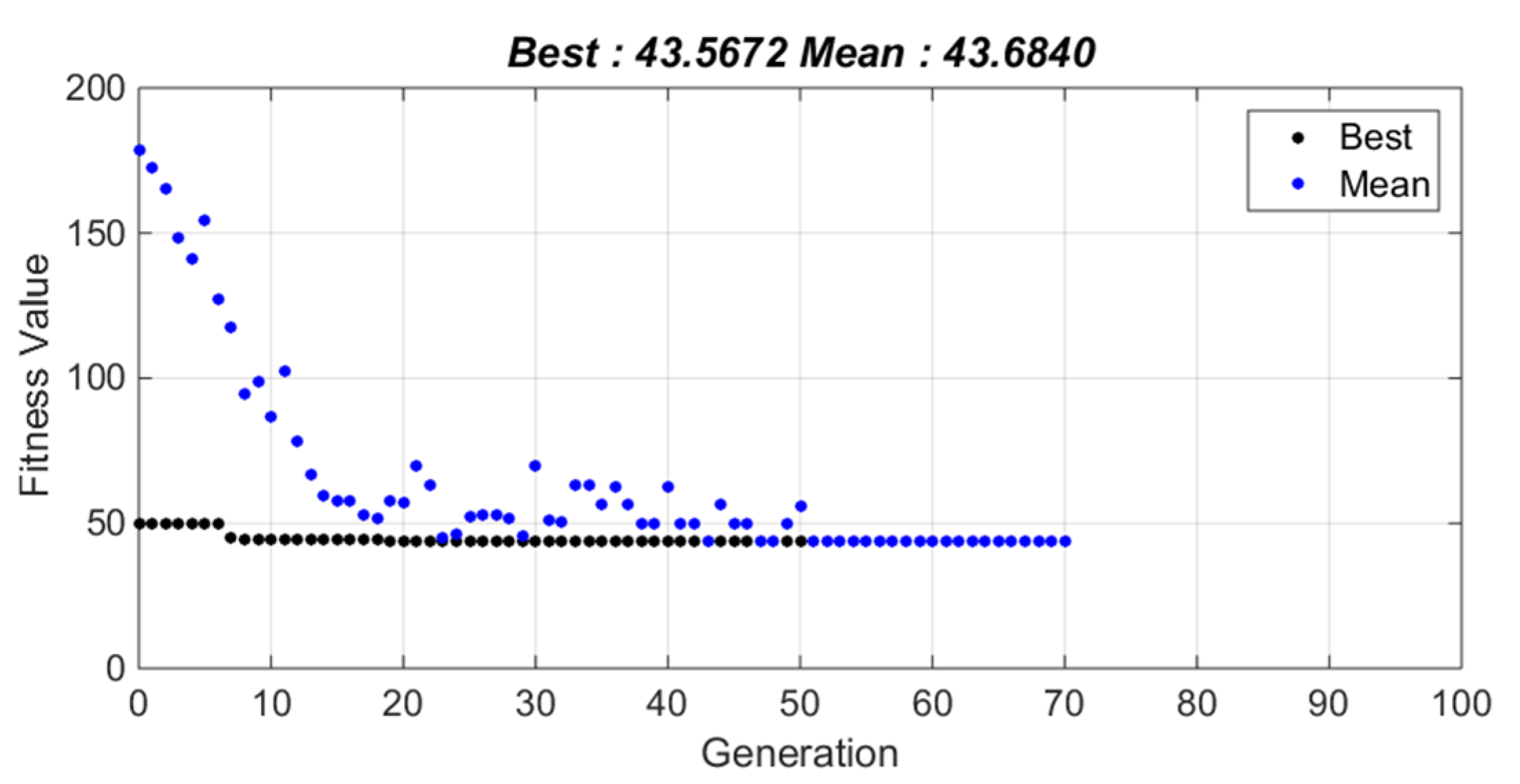
The increase in the mass of the battery and total mass of the UAV owing to the additional time of flight is highly significant. Design-1 has a battery mass of 1.2 kg and a total mass of 4.22 kg. With the addition of $t_{Enight}$ of 1.4 h, Design-2 has a battery mass of 1.52 kg and total mass of 5.04 kg. The further addition of a $t_{exc}^{req}$ of 5.56 h and minimum SOC of 10% increases the battery mass to 3.4 kg and total mass to 7.1 kg. The convergence of the objective function is presented in Figure 7. The mean and best values of the objective function for the last 20 generations are almost equal. This implies that all the configurations in the generation are identical. One design iteration requires 45 s on a personal i5 laptop with 16 GB RAM and 2.43 GHz processor. A total of 100 generations with 25 population sizes may require more than one day.

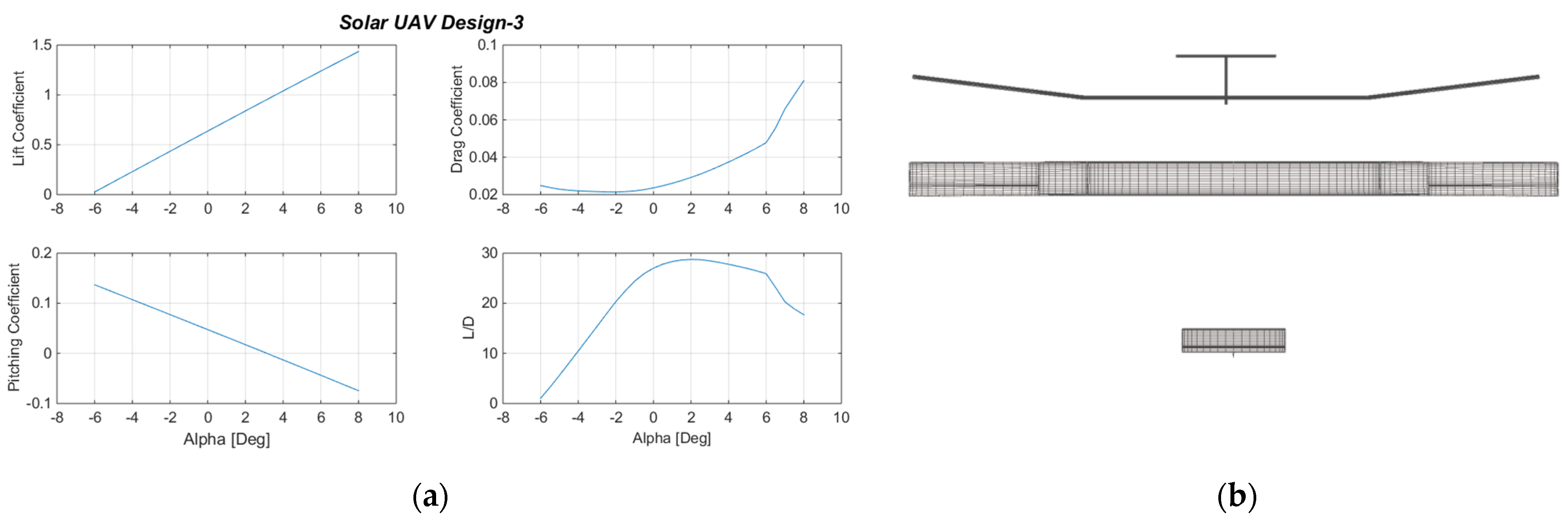
The lift, drag, and pitching moment coefficients and the lift-to-drag ratio of the optimized configuration are shown in Figure 8a. The trim angle of attack is 3.1°, where the pitching moment is zero. For this trim angle of attack, the lift coefficient is 0.96, and the lift-to-drag ratio is 28.4 (which is nearly the maximum for this design). The Xflr5 model showing panels’ density and control surfaces is also shown in Figure 8b.

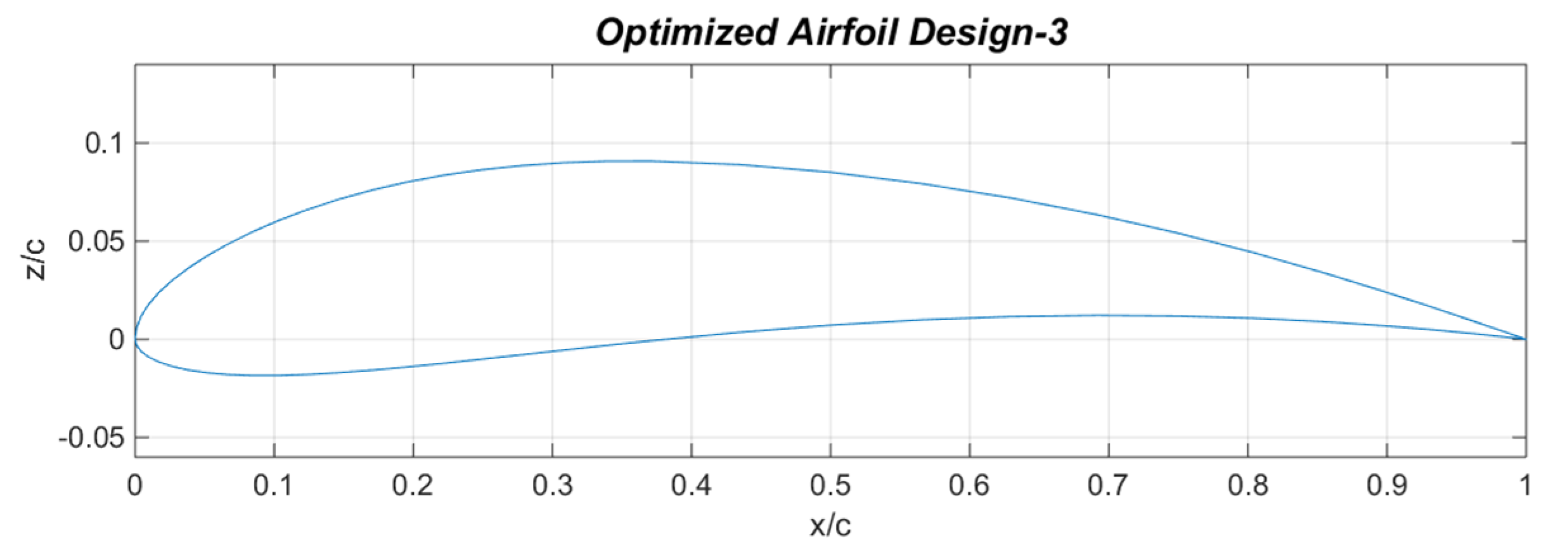
The optimized airfoil, shown in Figure 9, has a thickness of 9.7% at 25% and a maximum camber of 4.6% at 43.5% of the chord. The airfoil is highly smooth, and the trailing edge quality is good.

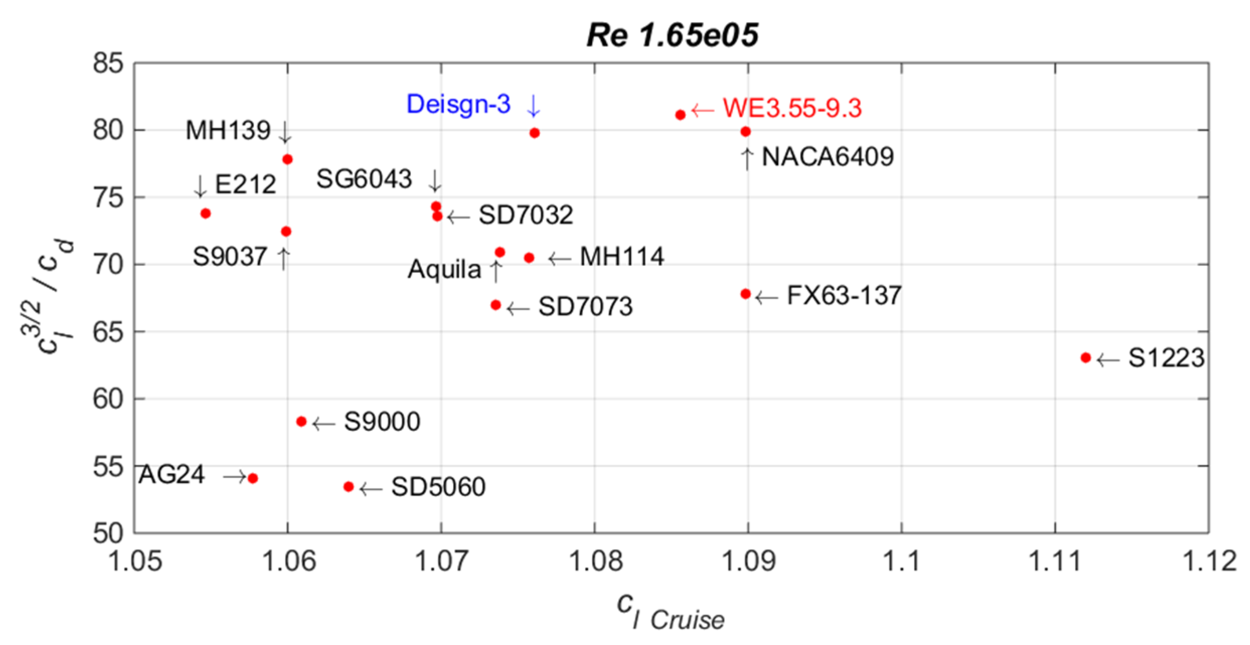
For Design-3, the wing incidence is set at 2°. As the steady-state alpha for Design-3 is 3.1°, the wing airfoil encounters a local incidence of 5.1° with a lift coefficient of 1.07. The Reynolds number for a cruise speed of 8.5 m/s is 1.65 × 10⁵. Fifteen different airfoils suggested for solar UAVs in the literature are analyzed in Xflr5 at a Reynolds number of 1.65 × 10⁵. $c{l}^{3/2}/cd$ for these airfoils for a lift coefficient of approximately 1.07 are plotted in Figure 10. The performance of optimized airfoil is higher than most of the airfoils and very close to Sky-Sailor [5] airfoil. This plot clearly shows the importance of airfoil selection with regard to the design lift coefficient and drag coefficient. These airfoils can be used for this lift coefficient, but a few airfoils evidently operate at higher $c{l}^{3/2}/cd$.

The energy simulation for 21 June is presented in Figure 11a. The SOC is also shown in black color. The solar UAV takes off at 07:00 with a completely drained battery ($SOC=0$). The available solar power is higher than the required power. The batteries become completely charged ($SOC=1$) within 6 h. The available solar energy can be used to attain an altitude or increase speed. At approximately 19:00, the available solar power is less than that required, and the batteries start to supply energy. At 20:00, solar power becomes unavailable, and the UAV operates completely on batteries. The next morning, when the solar power is higher than required, the batteries show a remaining capacity of 335 Wh. This corresponds to an SOC of 0.41.

A similar simulation for 1 May is also presented in Figure 11b. Owing to the lower solar irradiation on 1 May, the battery takes a longer time to charge fully. More battery is consumed to perform full-night flight because of the increased night hours. The next morning, when the available solar power is equal to the required power, the battery shows a minimum SOC of 0.37. It is concluded that Design-3 has the potential to perform continuous flight operations. However, it is important to note that the charge margin time [7] is reduced owing to the date change.

5. Dynamic Stability and Control System Design

In this section, the response of the optimized solar-powered UAV (Design-3) is discussed by applying the linearized equation of motion. These equations are based on small perturbations from the trim conditions. Additionally, these equations are decoupled. That is, the perturbations in longitudinal forces and moments depend neither on the lateral/directional perturbations nor the lateral/directional control inputs, and the perturbations in lateral/directional forces and moments depend neither on the longitudinal perturbations nor the longitudinal control inputs. Altitude hold and bank to turn control (BTT) systems are developed. The proposed control laws are then implemented in the nonlinear 6-DOF Matlab block for validation.

The first step is to estimate the moments of inertia. As the proposed optimization framework provides only the C.G. location for the desired static margin, a reasonable mass distribution that provides the required C.G. location is assumed. This distribution is passed on to Xflr5 to calculate the moments of inertia [40]. For Design-3, the neutral point and C.G. location are 0.72 m and 0.675 m, respectively (origin at fuselage nose). This yields a static margin of 15%. The estimated mass distribution is shown in Figure 12.

5.1. Attitude and Altitude Control

The linearized small disturbance longitudinal rigid body equations of motion in the state-space form are [41]:

$${\dot{x}}_{long}=A_{long}{x}_{long}+B_{long}{\eta }_{long}$$

(24)

where

$$A_{long}=\left[\begin{array}{cccc}{X}_u& X_w& 0& -g_{0}cos{\mathrm{\theta }}_0\\ Z_u& Z_w& u_0+Z_q& -g_{0}sin{\mathrm{\theta }}_0\\ M_u+M_{\dot{w}}{Z}_u& M_w+M_{\dot{w}}{Z}_w& M_q+u_0{M}_{\dot{w}}& -M_{\dot{w}}{g}_{0}sin{\mathrm{\theta }}_0\\ 0& 0& 1& 0\end{array}\right]$$

(25)

and

$$B_{long}=\left[\begin{array}{cc}{X}_{{\delta }_e}& X_{{\delta }_T}\\ Z_{{\delta }_e}& Z_{{\delta }_T}\\ M_{{\delta }_e}+M_{\dot{w}}{Z}_{{\delta }_e}& M_{{\delta }_T}+M_{\dot{w}}{Z}_{{\delta }_T}\\ 0& 0\end{array}\right]$$

(26)

The longitudinal state variable vector, $x_{long}$, is given by:

$$x_{long}={\left[\begin{array}{ccc}u& w& \begin{array}{cc}q& \theta \end{array}\end{array}\right]}^T$$

(27)

where $u$, $w$, $q$, and $\theta$ are the forward velocity, vertical velocity, pitch rate, and pitch angle, respectively. A longitudinal control vector, ${\eta }_{long}$, is given by:

$${\eta }_{long}={\left[\begin{array}{cc}{\delta }_e& {\delta }_T\end{array}\right]}^T$$

(28)

${\delta }_e$ and ${\delta }_T$ are perturbations from the trim in the elevator and throttle settings, respectively. Xflr5 is used to calculate the stability and control derivatives. Xflr5 predictions can be used for preliminary design analysis. These predictions can be improved using high fidelity tools or wind tunnel testing. The definitions and relationships between the dimensional stability derivatives for longitudinal dynamics and dimensionless derivatives of aerodynamic coefficients are presented in [40,41]. The longitudinal derivatives for Design-3 are listed in

Table 7. Longitudinal derivatives of aerodynamic coefficients.

Derivatives	Value
$C_X{}_u$	−0.051647
$C_X{}_{\alpha }$	0.6825
$C_z{}_u$	0.00659
$C_L{}_{\alpha }$	5.7669
$C_L{}_q$	7.5009
$C_M{}_u$	−0.00684
$C_M{}_{\alpha }$	−1.424
$C_M{}_q$	−21.431

. XFLR5 does not compute derivatives with respect to $\dot{w}$. Hence, these are assumed to be zero.

The resulting plant matrix is given by:

$$A_{long}=\left[\begin{array}{cccc}-0.0625& 0.8259& 0& -9.81\\ -2.3014& -7.0192& 7.1385& 0\\ -0.0326& -5.4389& -15.30& 0\\ 0& 0& 1& 0\end{array}\right]$$

(29)

The eigenvalues of the longitudinal plant matrix A are −11.13 + 4.68i, −11.13 − 4.68i, −0.068 + 0.91i, and −0.068 − 0.91i, which corresponds to a short period and the phugoid mode. The short-period mode has a relatively short time period and is generally damped substantially. The phugoid mode has a significantly longer time period and is damped marginally. The properties of the short period and phugoid mode of the present system are given in

Table 8. Properties of short period and phugoid mode for Design-3.

Mode	$\mathit{D}\mathit{u}\mathit{m}\mathit{p}\mathit{i}\mathit{n}\mathit{g} \mathit{R}\mathit{a}\mathit{t}\mathit{i}\mathit{o} \mathit{\zeta }$	$\mathit{N}\mathit{a}\mathit{t}\mathit{u}\mathit{r}\mathit{a}\mathit{l} \mathit{F}\mathit{r}\mathit{e}\mathit{q}\mathit{u}\mathit{e}\mathit{n}\mathit{c}\mathit{y} \mathit{\omega } \left[{\mathrm{s}}^{-1}\right]$	$\mathit{P}\mathit{e}\mathit{r}\mathit{i}\mathit{o}\mathit{d} \mathit{T} \left[\mathrm{s}\right]$
Short-Period Mode	0.923	12.07	1.32
Phugoid Mode	0.074	0.91	6.93

.

In the attitude and altitude control system design, it is assumed that the forward velocity is controlled by a separate controller and maintained constant at 8.5 m/s. The engine control and actuator dynamics are omitted for simplicity. Control surfaces are modeled as simple trailing edge flaps with x and y hinge position at 70% of chord and 50% of thickness, respectively. The control surface sizing can be refined using high fidelity tools. The resulting state-space model is expressed as:

$$\left[\begin{array}{c}\Delta \dot{w}\\ \Delta \dot{q}\\ \Delta \dot{\theta }\end{array}\right]=\left[\begin{array}{ccc}-7.0192& 7.1385& 0\\ -5.4389& -15.30& 0\\ 0& 1& 0\end{array}\right]+\left[\begin{array}{c}-3.206\\ -59.29\\ 0\end{array}\right]\left[\theta {\delta }_e\right]$$

(30)

Figure 13a shows the longitudinal open-loop step response. The vertical velocity and pitch rate have non-zero values. The pitch angle continues to decrease dramatically. Therefore, a controller must be designed for the desired pitch angle response. In this study, a linear quadratic regulator (LQR) controller is used to determine the gains for the feedback loop. The goal is to identify a control vector $\eta \left(t\right)$ that drives the state from a specified initial state $x\left(t\right)$ to a desired final state $x_d\left(t_f\right)$ such that a specified performance index ($J$) is minimized:

$$J={{\displaystyle \int }}_t^{t_f}g\left(x\left(\tau \right),\eta \left(\tau \right),\tau \right)d\tau$$

(31)

where $g$ is specified as

$$g=x^{T}Qx+{\eta }^{T}R\eta$$

(32)

where $Q$ is a positive semi-definite weight matrix and $R$ is a positive-definite weight matrix. $Q$ and $R$ are selected to provide the optimal response as desired by the designer. For this design:

$$Q=\left[\begin{array}{ccc}0& 0& 0\\ 0& 0& 0\\ 0& 0& 1\end{array}\right] and R=\left[1\right]$$

(33)

The corresponding gain vector is given by:

$$K_{long}=\left[\begin{array}{ccc}0.0271& -0.0482& -1.0\end{array}\right]$$

(34)

The feedback response for the attitude-hold control system in response to a 1° step input is shown in Figure 13b. The rise and settling time of the pitch angle are 0.784 s and 1.48 s, respectively, with zero steady-state error. As the designed solar UAV must demonstrate exceptional endurance at a constant altitude, an altitude-hold control system is required. To design this system, we introduce a vertical height equation [41] in the current state-space model.

$$\Delta \dot{h}=u_0\left(\Delta \theta -\Delta \alpha \right)$$

(35)

The resulting state space model is given as:

$$\left[\begin{array}{c}\Delta \dot{\alpha }\\ \Delta \dot{q}\\ \begin{array}{c}\Delta \dot{\theta }\\ \Delta \dot{h}\end{array}\end{array}\right]=\left[\begin{array}{ccc}-7.019& 0.8398& \begin{array}{cc}0& 0\end{array}\\ -46.23& -15.305& \begin{array}{cc}0& 0\end{array}\\ \begin{array}{c}0\\ -8.5\end{array}& \begin{array}{c}1\\ 0\end{array}& \begin{array}{c}\begin{array}{cc}0& 0\end{array}\\ \begin{array}{cc}8.5& 0\end{array}\end{array}\end{array}\right]+\left[\begin{array}{c}-0.377\\ -59.29\\ \begin{array}{c}0\\ 0\end{array}\end{array}\right]\left[\Delta {\delta }_e\right]$$

(36)

The corresponding LQR gains are [0.2308 − 0.0482 − 1.000], which correspond to the state alpha, pitch rate, and pitch angle, respectively. This system is the same as Equation (30), except vertical velocity is replaced by alpha. A PID controller is suggested in the outer loop that would generate a theta command resulting from the difference between the target height and current height. The parameters of the PID controller are $P=0.07025, I=0.0003309, D=-0.0300, \mathrm{and} N=0.5372$. The response to the 1 m step input is shown in Figure 14. The linear pitch angle accurately matches the pitch angle command, and the target height is achieved with zero steady-state error. The maximum elevator deflection to produce desired pitch angle is 1°.

5.2. Heading Control

The linearized small disturbance lateral rigid body equations of motion in state-space form are given by [41]:

$${\dot{x}}_{lat}=A_{lat}{x}_{lat}+B_{lat}{\eta }_{lat}$$

(37)

where

$$A_{lat}=\left[\begin{array}{cccc}{Y}_v& Y_p& g_0\cos {\mathsf{\Theta }}_0& Y_r-u_0\\ L_v& L_p& 0& L_r\\ 0& 1& 0& 0\\ N_v& N_p& 0& N_r\end{array}\right] and B_{lat}=\left[\begin{array}{cc}{Y}_{{\delta }_r}& Y_{{\delta }_a}\\ L_{{\delta }_r}& L_{{\delta }_a}\\ 0& 0\\ N_{{\delta }_r}& N_{{\delta }_a}\end{array}\right]$$

(38)

Lateral state vector $x_{lat}$ and input control vector ${\eta }_{lat}$ are given by:

$$x_{lat}={\left[\begin{array}{cccc}v& p& \varphi & r\end{array}\right]}^T, {\eta }_{lat}={\left[\begin{array}{cc}{\delta }_r& {\delta }_a\end{array}\right]}^T$$

(39)

where $v$, $p$, $\varphi$ and $r$ are the lateral velocity, roll rate, roll angle and yaw rate, respectively. ${\delta }_r$ and ${\delta }_a$ are the perturbations from trim in the rudder and aileron. It is also convenient to replace lateral velocity with sideslip angle,$\beta$, using the following relationship.

$$\beta \cong \tan \beta =\frac{v}{V_0}$$

(40)

The resulting plant matrix is given by [42]:

$$A_{lat}=\left[\begin{array}{cccc}{Y}_v& Y_p/V_0& \left(g_0\cos {\mathsf{\Theta }}_0\right)/V_0& \left(Y_r-u_0\right)/V_0\\ L_v{V}_0& L_p& 0& L_r\\ 0& 1& 0& 0\\ N_v{V}_0& N_p& 0& N_r\end{array}\right]$$

(41)

The dynamics of the resulting system are the same as those of the original system except that the state vector is now ${\left[\begin{array}{ccc}\beta & p& \begin{array}{cc}\varphi & r\end{array}\end{array}\right]}^T$. For heading angle control, both skid to turn (STT) and bank to turn can be implemented. In STT, rudders are the primary control surface. Rudders are used to create sideslip and aircraft turns in the direction of rudder deflection. Ailerons can be used to encounter roll produced due to yaw and to keep the wings level if desired. In BTT, ailerons are the primary control surface. Ailerons are deflected to bank the aircraft into a turn. In the current study, a BTT maneuver is modeled. Lateral aerodynamic derivatives estimated using Xflr5 are listed in

Table 9. Lateral derivatives of aerodynamic coefficients.

Derivatives	Value
$C_Y{}_{\beta }$	−0.2339
$C_Y{}_p$	−0.2156
$C_Y{}_r$	0.1841
$C_l{}_{\beta }$	−0.1193
$C_l{}_p$	−0.7429
$C_l{}_r$	0.2709
$C_n{}_{\beta }$	0.0277
$C_n{}_p$	−0.1431
$C_n{}_r$	−0.0231

.

The lateral dynamics are complex as compared to longitudinal dynamics, involving one force and two moments. Eigenvalues of lateral plant matrix $A_{lat}$ are −26.09, −1.47 + 2.12i, −1.47 − 2.12i and 0.116, which corresponds to roll subsidence, Dutch roll and spiral mode, respectively. The positive value of the spiral mode indicates that it is unstable. Before designing a linear BTT control system, we must first add the BTT equation to our system. The BTT equation is given by:

$$r\approx \frac{g}{V_0}\varphi$$

(42)

It states that any non-zero roll angle will induce a yaw rate. This equation can be incorporated into state-space using $\dot{\psi }=r$. After augmenting the BTT equation in Equation (41), the plant matrix and control matrix are given by:

$$A_{lat}=\left[\begin{array}{ccccc}-0.2831& -0.0896& 1.1541& -0.9235& 0\\ -13.0276& -27.8583& 0& 10.1602& 0\\ 0& 1.0000& 0& 0& 0\\ 2.7068& -4.8078& 0& -0.7767& 0\\ 0& 0& 1.1529& 0& 0\end{array}\right] and B_{lat}=\left[\begin{array}{c}0.1696\\ 50.0247\\ 0\\ -0.0064\\ 0\end{array}\right]$$

(43)

Like longitudinal control, LQR is used to model the BTT maneuver. Q and R matrix are:

$$Q=\left[\begin{array}{ccccc}10& 0& 0& 0& 0\\ 0& 80& 0& 0& 0\\ 0& 0& 30& 0& 0\\ 0& 0& 0& 5& 0\\ 0& 0& 0& 0& 8\end{array}\right] and R=\left[1\right]$$

(44)

Weights in the Q matrix are selected to obtain the optimum response for all the states. The corresponding LQR gains are $K_{lat}$= [1.4579 8.4355 11.8906 −0.9540 2.8284]. The poles of the closed loop system $\left(A_{lat}-B_{lat}{K}_{lat}\right)$ are −448.2, −1.03 + 1.6i, 1.03 − 1.6i, −0.45 + 0.28i and −0.45 − 0.28i. All the roots are now negative; hence, the system is now stable. The response to a 110° turn is shown in Figure 15. The yaw rate is limited to 2°/s.

5.3. Six-DOF Non-Linear Simulation

The proposed control strategy is validated in the 6-DOF Matlab Simulink model. The aerodynamic model used for this simulation is presented below.

$$L=C_L\overline{q}S where C_L=C_{L_0}+C_{L_{\alpha }}\alpha +\frac{\overline{c}}{2V}{C}_{L_q}q+C_{L_{\delta e}}\delta e$$

$$D=C_D\overline{q}S where C_D=C_{D_0}+C_{D_{\alpha }}\alpha +C_{D_{\delta e}}\delta e$$

$$M_A=C_m\overline{q}S\overline{c} where C_m=C_{m_0}+C_{m_{\alpha }}\alpha +\frac{\overline{c}}{2V}{C}_{m_q}q+C_{m_{\delta e}}\delta e$$

$$L_A=C_l\overline{q}Sb where C_l=C_{l_0}+C_{l_{\beta }}\beta +\frac{b}{2V}{C}_{l_p}p+\frac{b}{2V}{C}_{l_r}r+C_{l_{\delta a}}\delta a+C_{l_{\delta r}}\delta r$$

$$N_A=C_n\overline{q}Sb where C_n=C_{n_0}+C_{n_{\beta }}\beta +\frac{b}{2V}{C}_{n_p}p+\frac{b}{2V}{C}_{n_r}r+C_{n_{\delta a}}\delta a+C_{n_{\delta r}}\delta r$$

$$Y=C_Y\overline{q}S where C_Y=C_{Y_0}+C_{Y_{\beta }}\beta +\frac{b}{2V}{C}_{Y_p}p+\frac{b}{2V}{C}_{Y_r}r+C_{Y_{\delta a}}\delta a+C_{Y_{\delta r}}\delta r$$

where $L$, $D$, $M_A$, $L_A$, $N_A$, $Y$, $\overline{q}$ and $\overline{c}$ are lift, drag, pitching moment, rolling moment, yawing moment, side force, dynamic pressure and mean aerodynamic chord, respectively. $C_{L_0}$, $C_{D_0}$, $C_{m_0}$, $C_{l_0}$, $C_{n_0}$ and $C_{Y_0}$ are lift, drag, pitching, rolling, yawing and side force coefficient at $\alpha =\delta e=\beta =\delta a=\delta r=0$, respectively. The final trajectory is to climb to an altitude of 350 m at the rate of 2 m/s, after being hand-launched from an initial altitude of 0 m. After climbing to 350 m, there is a small cruise segment. At t = 250 s, the UAV starts a climbing turn, climbing with a rate of 1 m/s and turning with a yaw rate of 2°/s. After climbing to 700 m, the UAV holds this altitude and continues to fly in a circular path with the same yaw rate. As noted in Figure 15, the BTT maneuver also produces a sideslip angle. In the 6-DOF simulation, the rudder is used to encounter the sideslip angle using a proportional controller, often known as a coordinated turn. Throughout the trajectory, the velocity of 8.5 m/s is maintained. To account for any expected sensor noises, the Matlab Simulink built-in band limited white noise model is used (Figure 16).

The angle of attack and sideslip angle are shown in Figure 17a. At the final cruise altitude of 700 m, alpha is around 3.2°, which is consistent with static analysis and design. Sideslip is zero throughout the trajectory. In Figure 17b, x and y coordinates are plotted to visualize the circular motion. For the given yaw rate of 2°/s, the UAV flies in a circular path with 480 m diameter.

The height profile of the solar UAV with axial location is also shown in Figure 18a. After reaching the target height of 700 m, the UAV successfully maintains this altitude. Euler angles are also presented in Figure 18b. During climbing turn, the pitch angle is around 10°. After achieving a target height, the pitch angle is reduced to 3.2°, which is equal to the angle of attack. Hence, the solar UAV is flying with zero flight path angle. For the yaw angle, the range of the plot is −180° to 180° (one complete circle). To elaborate, the trajectory of the solar UAV is shown in a 3D plot (Figure 19). Different segments of the trajectory are shown with different colors.

6. Conclusions

In this paper, the genetic algorithm is used to optimize a solar-powered UAV for a specific height, cruise speed and static margin. The wing airfoil is also considered as a design variable and a new structural mass estimation model is proposed. This model also caters for the change in structural mass with the change in wing airfoil during optimization. The objective is to design an airfoil for specified flight conditions, considering overall performance and weight estimation. To add robustness in the design, an extra battery is added as the system starts to consume the battery as soon as the required power is lower than the available solar power. The optimized configuration has a total mass of 7.08 kg with a battery mass of 3.4 kg. The optimized airfoil is very smooth, with a thickness and camber of 9.7% and 4.6%, respectively. To ensure control and handling, dynamic stability and control systems are also discussed using linearized equations of motion. The control laws are developed using an LQR and PID controller. The designed altitude and BTT controllers are implemented in a closed-loop nonlinear 6-DOF simulation. The results of the 6-DOF simulation are in good agreement with linear static analysis, validating the complete design process.

References

1. Predator RQ-1/MQ-1/MQ-9 Reaper UAV. Available online: https://www.airforce-technology.com/projects/predator-uav/ (accessed on 4 March 2021).
2. Global Hawk-Northrop Grumman. Available online: https://www.northropgrumman.com/what-we-do/air/globalhawk-rq-4-unmanned-aircraft-system (accessed on 4 March 2021).
3. Zephyr Solar-Powered HALE UAV-Airforce Technology. Available online: https://www.airforce-technology.com/projects/zephyr/ (accessed on 4 March 2021).
4. Ackerman, E. Giant Solar-Powered UAVs Are Atmospheric Satellites. Available online: https://spectrum.ieee.org/automaton/robotics/drones/giant-solar-powered-uavs-are-atmospheric-satellites (accessed on 4 March 2021).
5. Andre, N. Design of Solar Powered Airplanes for Continuous Flight. Ph.D. Thesis, ETH Zurich, Zurich, Switzerland, 2008. [Google Scholar]
6. Solong UAV: First Solar-Powered Perpetual Flight in History. Available online: https://archive.org/details/ACPropulsionSolongUAV2005/ (accessed on 4 March 2021).
7. Oettershagen, P.; Melzer, A.; Mantel, T.; Rudin, K.; Lotz, R.; Siebenmann, D.; Leutenegger, S.; Alexis, K.; Siegwart, R. A solar-powered hand-launchable UAV for low-altitude multi-day continuous flight. In Proceedings of the 2015 IEEE International Conference on Robotics and Automation (ICRA), Seattle, WA, USA, 26–30 May 2015; pp. 3986–3993. [Google Scholar]
8. Sri, K.R.B.; Aneesh, P.; Bhanu, K.; Natarajan, M. Design analysis of solar-powered unmanned aerial vehicle. J. Aerosp. Technol. Manag. 2016, 8, 397–407. [Google Scholar] [CrossRef]
9. Betancourth, N.J.P.; Villamarin, J.E.P.; Rios, J.J.V.; Bravo-Mosquera, P.D.; Cerón-Muñoz, H.D. Design and manufacture of a solar-powered unmanned aerial vehicle for civilian surveillance missions. J. Aerosp. Technol. Manag. 2016, 8, 385–396. [Google Scholar] [CrossRef] [Green Version]
10. Jiajan, W.; Kampoon, J.; Klongtrujrok, J.; Yuthayanon, I. Conceptual Design of Tactical Solar Power UAV. IOP Conf. Ser. Mater. Sci. Eng. 2019, 501, 012011. [Google Scholar] [CrossRef]
11. Leutenegger, S.; Jabas, M.; Siegwart, R.Y. Solar airplane conceptual design and performance estimation: What size to choose and what endurance to expect. J. Intell. Robot Syst. Theory Appl. 2011, 61, 545–561. [Google Scholar] [CrossRef]
12. Ahn, H.; Ahn, J. Design and Analysis of a Solar-Power Mini-UAV for Extended Endurance at Low Altitude. Int. J. Aeronaut. Space Sci. 2019, 20, 561–569. [Google Scholar] [CrossRef]
13. Rajendran, P.; Smith, H. Development of design methodology for a small solar-powered unmanned aerial vehicle. Int. J. Aerosp. Eng. 2018, 2018, 2820717. [Google Scholar] [CrossRef] [Green Version]
14. Escobar-Ruiz, A.G.; Lopez-Botello, O.; Reyes-Osorio, L.; Zambrano-Robledo, P.; Amezquita-Brooks, L.; Garcia-Salazar, O. Conceptual Design of an Unmanned Fixed-Wing Aerial Vehicle Based on Alternative Energy. Int. J. Aerosp. Eng. 2019, 2019, 8104927. [Google Scholar] [CrossRef]
15. Harasani, W.; Khalid, M.; Arai, N.; Fukuda, K.; Hiraoka, K. Initial conceptual design and wing aerodynamic analysis of a solar power-based UAV. Aeronaut. J. 2014, 118, 540–554. [Google Scholar] [CrossRef]
16. Dwivedi, V.S.; Patrikar, J.; Addamane, A.; Ghosh, A.K. MARAAL: A Low Altitude Long Endurance Solar Powered UAV for Surveillance and Mapping Applications. In Proceedings of the 2018 23rd International Conference on Methods & Models in Automation & Robotics (MMAR), Miedzyzdroje, Poland, 27–30 August 2018; pp. 449–454. [Google Scholar]
17. Shiau, J.K.; Ma, D.M. Development of an experimental solar-powered unmanned aerial vehicle. J. Chin. Inst. Eng. 2015, 38, 701–713. [Google Scholar] [CrossRef]
18. Morton, S.; D’Sa, R.; Papanikolopoulos, N. Solar powered UAV: Design and experiments. In Proceedings of the 2015 IEEE/RSJ International Conference on Intelligent Robots and Systems (IROS), Hamburg, Germany, 28 September–2 October 2015; pp. 2460–2466. [Google Scholar]
19. Zhao, X.; Zhou, Z.; Zhu, X.; Guo, A. Design of a hand-launched solar-powered unmanned aerial vehicle (UAV) system for plateau. Appl. Sci. 2020, 10, 1300. [Google Scholar] [CrossRef] [Green Version]
20. Marta André, C.; Gamboa Pedro, V. Long endurance electric UAV for civiliansurveillance missions. In Proceedings of the International Council of Aeronautical Science, St. Petersburg, Russia, 7–12 September 2014. [Google Scholar]
21. Guo, Z.; Chen, X.K.; Hou, Z.X.; Guo, J. Development of a solar electric powered UAV for long endurance flight. In Proceedings of the 11th AIAA Aviation Technology, Integration, and Operations (ATIO) Conference, Virginia Beach, VA, USA, 20–22 September 2011; pp. 1–13. [Google Scholar]
22. Bahrami Torabi, H.; Sadi, M.; Varjani, A.Y. Solar Power System for experimental unmanned aerial vehicle (UAV); Design and fabrication. In Proceedings of the 2011 2nd Power Electronics, Drive Systems and Technologies Conference, Tehran, Iran, 16–17 February 2011; pp. 129–134. [Google Scholar]
23. Feng, S.; Li, P.; Xue, Y.; Gao, F.; Bai, Z.; Zhang, L.; Guo, Q. Characteristics and design key points of small CIGS solar UAV. IOP Conf. Ser. Earth Environ. Sci. 2020, 508, 012208. [Google Scholar] [CrossRef]
24. Mattar, A.K.; Vaidya, C.; Saraf, A.M. Airfoil selection, optimization and analysis for a solar-powered unmanned aerial vehicles. In Proceedings of the 2016 IEEE Aerospace Conference, Big Sky, MT, USA, 5–12 March 2016; pp. 1–9. [Google Scholar]
25. Marques Hobold, G.; Agarwal, R.K. A methodology for predicting solar power incidence on airfoils and their optimization for solar-powered airplanes. Proc. Inst. Mech. Eng. Part G J. Aerosp. Eng. 2015, 229, 1267–1279. [Google Scholar] [CrossRef]
26. Gao, X.-Z.; Hou, Z.-X.; Guo, Z.-C.; Chen, X.-Q. Design and performance test of a twin fuselage configuration solar-powered UAV. In Proceedings of the 29th International Council of Aeronautical Science, St. Petersburg, Russia, 7–12 September 2014. [Google Scholar]
27. Berry, P. The sunriser-A design study in solar powered flight. In Proceedings of the 2000 World Aviation Conference, San Diego, CA, USA, 10–12 October 2000. [Google Scholar]
28. Stender, W. Sailplane Weight Estimation; Organisation Scientifique et Technique Internationale du Vol à Voile (OSTIV): Braunschweig, Germany, 1969. [Google Scholar]
29. Rizzo, E.; Frediani, A. A model for solar powered aircraft preliminary design. Aeronaut. J. 2008, 112, 57–78. [Google Scholar] [CrossRef]
30. Wilkins, G.; Fourie, D.; Meyer, J. Critical design parameters for a low altitude long endurance solar powered UAV. In Proceedings of the AFRICON 2009, Nairobi, Kenya, 23–25 September 2009; pp. 1–6. [Google Scholar]
31. Hartney, C. Conceptual Design of a Model Solar-Powered Unmanned Aerial Vehicle. In Proceedings of the 50th AIAA Aerospace Sciences Meeting including the New Horizons Forum and Aerospace Exposition, Nashville, Tennessee, 9–12 January 2012. [Google Scholar]
32. Jashnani, S.; Nada, T.R.; Ishfaq, M.; Khamker, A.; Shaholia, P. Sizing and preliminary hardware testing of solar powered UAV. Egypt J. Remote Sens. Space Sci. 2013, 16, 189–198. [Google Scholar] [CrossRef] [Green Version]
33. Weider, A.; Levy, H.; Regev, I.; Ankri, L.; Goldenberg, T.; Ehrlich, Y.; Vladimirsky, A.; Yosef, Z.; Cohen, M. SunSailor: Solar powered UAV. In Proceedings of the 47th Israel Annual Conference on Aerospace Sciences 2007, Tel Aviv-Haifa, Israel, 21–22 February 2007. [Google Scholar]
34. Hicks Raymond, M.; Henne Preston, A. Wing Design by Numerical Optimization. J. Aircr. 1978, 15, 407–412. [Google Scholar] [CrossRef]
35. Kulfan Brenda, M.; Bussoletti John, E. “Fundamental” parametric geometry representations for aircraft component shapes. In Proceedings of the 11th AIAA/ISSMO Multidisciplinary Analysis and Optimization Conference, Portsmouth, Virginia, 6–8 September 2006; pp. 547–591. [Google Scholar]
36. Sobieczky, H. Parametric Airfoils and Wings. In Notes on Numerical Fluid Mechanics; Fujii, K., Dulikravich, G.S., Eds.; Vieweg: Wiesbaden, Germany, 1999. [Google Scholar]
37. Aerodynamics and Aircraft Design Software. Available online: http://www.dept.aoe.vt.edu/~mason/Mason_f/MRsoft.html (accessed on 4 March 2021).
38. Kimura, K.; Stephenson, D.G. Solar radiation on cloudy days. Research Paper No. 418. Trans. Am. Soc. Heating Refrig. Air Cond. Eng. INC 1969, 75, 1040–1050. [Google Scholar]
39. Christopher, J. Orendorff, Dan Doughty. Lithium Ion Battery Safety Guidance. Massachusetts Institute of Technology. Available online: https://ehs.mit.edu/wp-content/uploads/2019/09/Lithium_Battery_Safety_Guidance.pdf (accessed on 4 March 2021).
40. Deperrois, A. Guidelines for XFLR5: Analysis of Foils and Wings Operating at Low Reynolds Numbers. Available online: https://engineering.purdue.edu/~aerodyn/AAE333/FALL10/HOMEWORKS/HW13/XFLR5_v6.01_Beta_Win32%282%29/Release/Guidelines.pdf (accessed on 4 March 2021).
41. Nelson, R.C. Flight Stability and Automatic Control, 2nd ed.; WCB/McGraw-Hill: New York, NY, USA, 1998. [Google Scholar]
42. Cook, V.M. Flight Dynamics Principles, 2nd ed.; Elsevier Ltd.: Amsterdam, The Netherlands, 2000. [Google Scholar]
Figure 1. Structural components of solar UAV: (a) Upper wing, (b) Lower wing, (c) Fuselage, (d) Wing rib.
Aerospace 08 00228 g001
Figure 2. Rib design for wing and tail airfoil.
Aerospace 08 00228 g002
Figure 3. CST representation of NACA 63–137 airfoils.
Aerospace 08 00228 g003
Figure 4. CST parameter for 15 airfoils recommended for solar UAVs.
Aerospace 08 00228 g004
Figure 5. Comparison of Xflr5 and experimental data, E387 at Re = 2.0 × 10⁵.
Aerospace 08 00228 g005
Figure 6. Energy simulation: (a) t n i g h t = 9.2   h , (b) t n i g h t = 9.2   h ,   t E n i g h t = 1.4   h .
Aerospace 08 00228 g006
Figure 7. Convergence history of objective function, Design-3.
Aerospace 08 00228 g007
Figure 8. (a) Lift, drag, moment, and L/D of Design-3, (b) Xflr5 model.
Aerospace 08 00228 g008
Figure 9. Optimized airfoil for Design-3.
Aerospace 08 00228 g009
Figure 10. Performance comparison of airfoils.
Aerospace 08 00228 g010
Figure 11. Design-3, energy simulation: (a) 21 June and (b) 1 May.
Aerospace 08 00228 g011
Figure 12. Mass distribution for required C.G. location, Design-3.
Aerospace 08 00228 g012
Figure 13. Longitudinal step response: (a) Open Loop, (b) Closed Loop.
Aerospace 08 00228 g013
Figure 14. Longitudinal outer-loop step response.
Aerospace 08 00228 g014
Figure 15. Heading angle control response for 110° reference.
Aerospace 08 00228 g015
Figure 16. Block diagram of current control system and implementation of noise.
Aerospace 08 00228 g016
Figure 17. Simulation results: (a) Alpha and Beta, (b) Circular Motion.
Aerospace 08 00228 g017
Figure 18. Simulation results: (a) Height Profile, (b) Euler Angles.
Aerospace 08 00228 g018
Figure 19. Solar UAV trajectory in 3D.
Aerospace 08 00228 g019