Neuro-Fuzzy Network-Based Reduced-Order Modeling of Transonic Aileron Buzz


Abstract
:1. Introduction
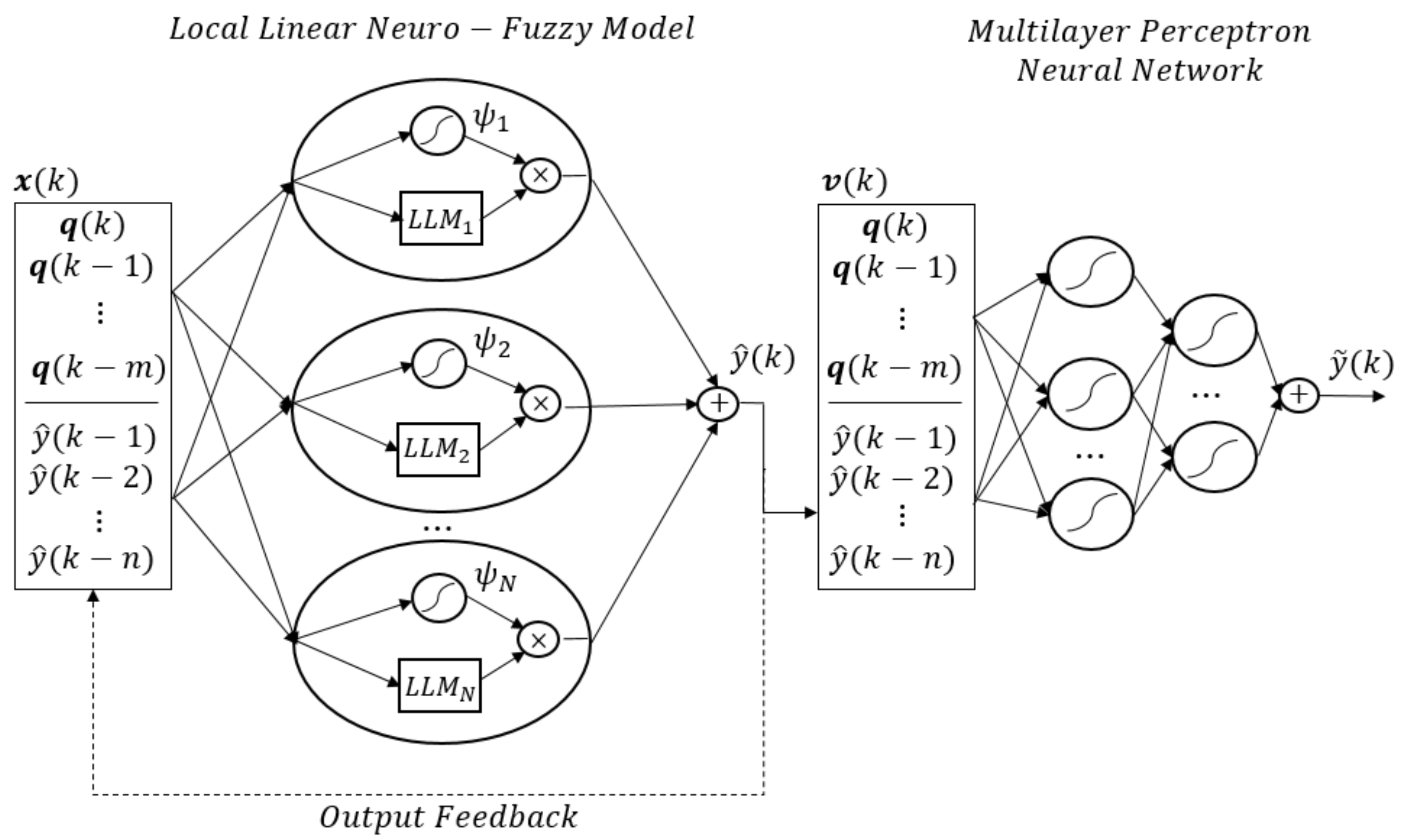
2. Reduced-Order Model Approach
- Model Initialization: As a first step, a global linear model () is calculated by estimating the NFM weights () by means of a local linear least-squares algorithm [25]. Therefore, the available CFD training data set is applied.
- LLM error estimation: Within the next step, the worst performing local linear model is located by means of a locally-defined loss function, which is evaluated for all available models (). The LLM yielding the highest prediction error is selected for the subsequent splitting procedure [12]. If only the global model is available, it is automatically chosen for further refinement.
- LLM refinement: The LLM which shows the lowest performance is divided into two models using an axis-orthogonal split [25]. For each resulting model, the centers (), widths () and weights () must be re-computed. The centers are defined as the centers of the corresponding jth hyperrectangle, while the widths are determined by defining the input space extension of the LLM scaled by a factor [12]. According to Nelles [25], is chosen as . The linear weights are determined by the application of the local weighted least-squares optimization.
- Error evaluation: In order to evaluate the best splitting configuration, a loss function is applied. Therefore, in contrast to the weight estimation procedure in training step one, the available validation data set is applied. Based on the error evaluation, the partition-setup yielding the lowest error is chosen for the last training step.
- Termination: The aforementioned training steps are repeated until the relative change of the error as calculated in the previous step becomes smaller than a user-defined value. As an alternative, the splitting process can be terminated by defining a maximum number of LLMs [12].
3. Structural and Numerical Setup
3.1. Structural Model
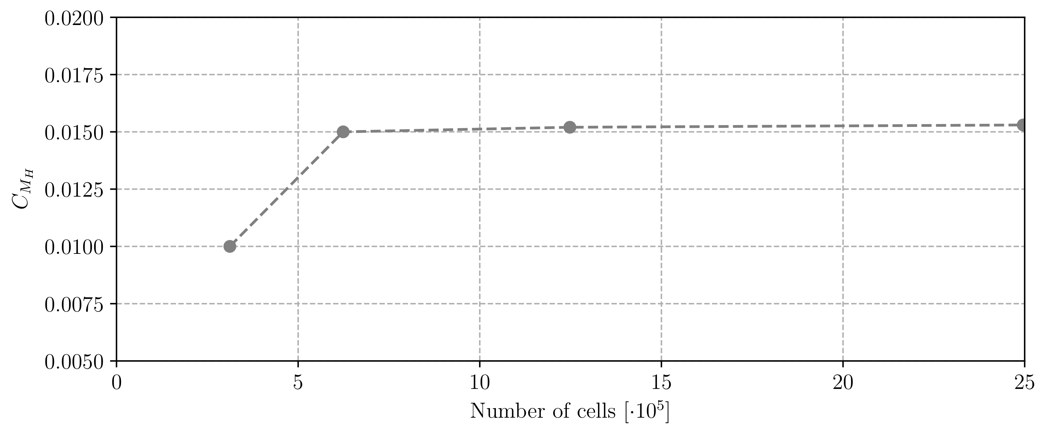
3.2. CFD-Solver
4. Application
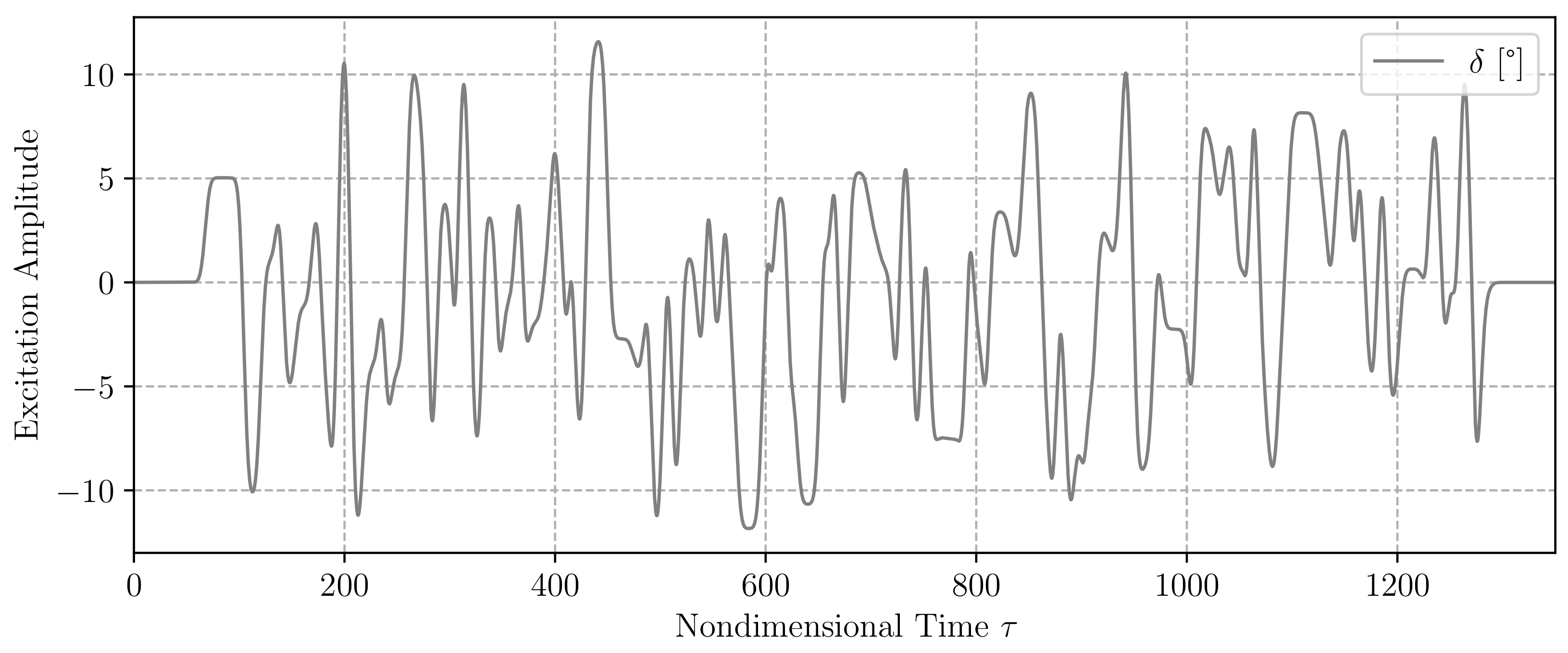
4.1. Training Data Generation
4.2. Nonlinear System Identification
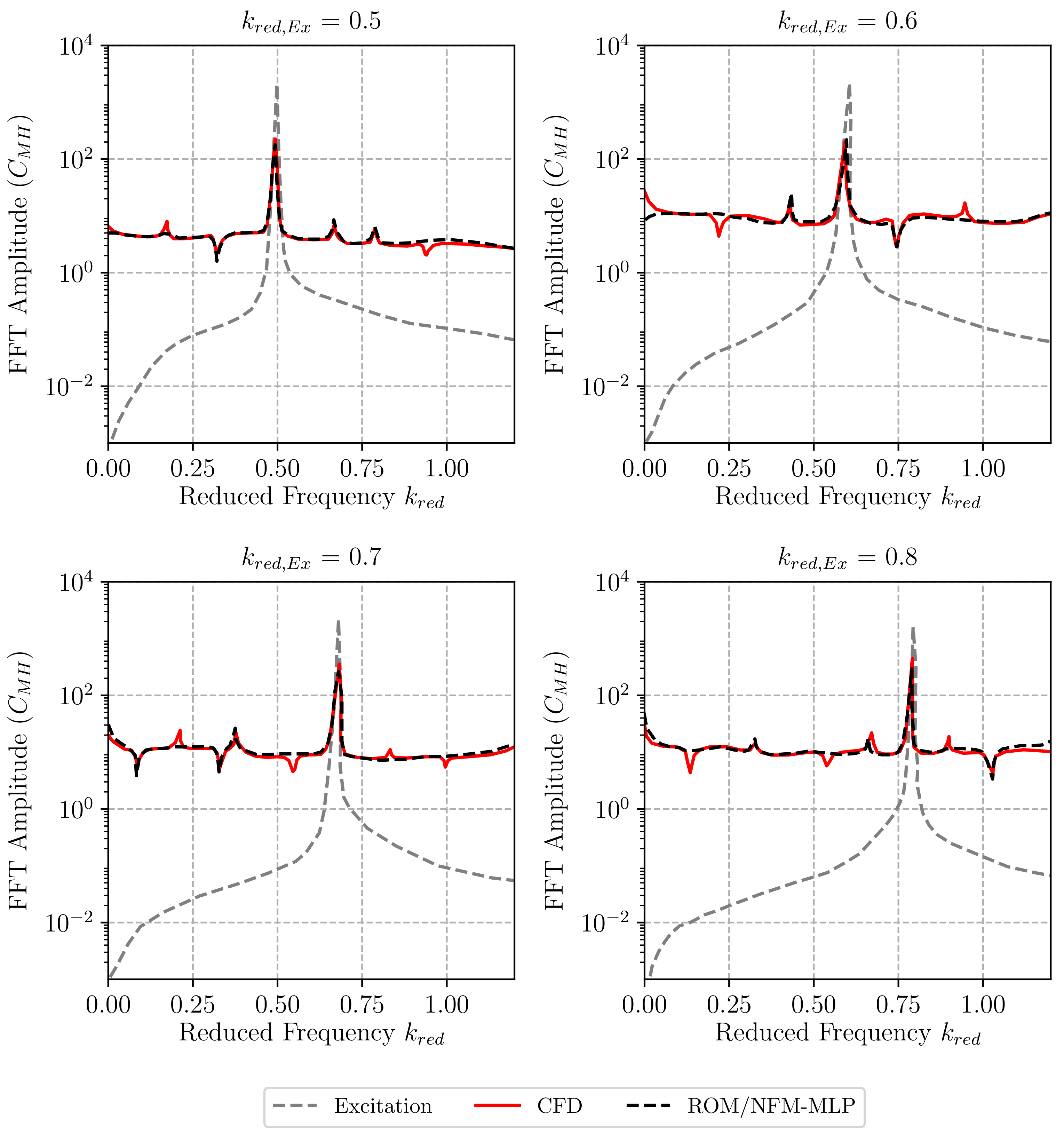
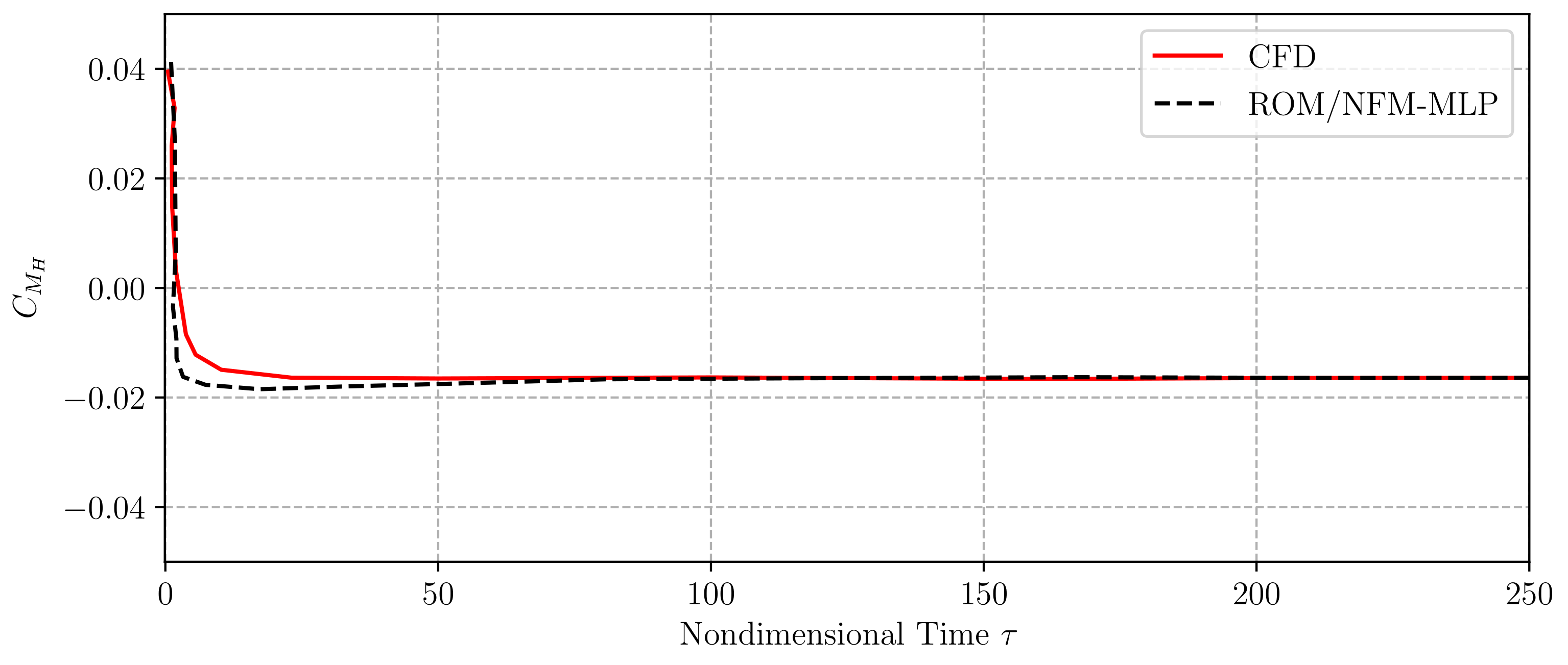
4.2.1. Aerodynamic System Identification
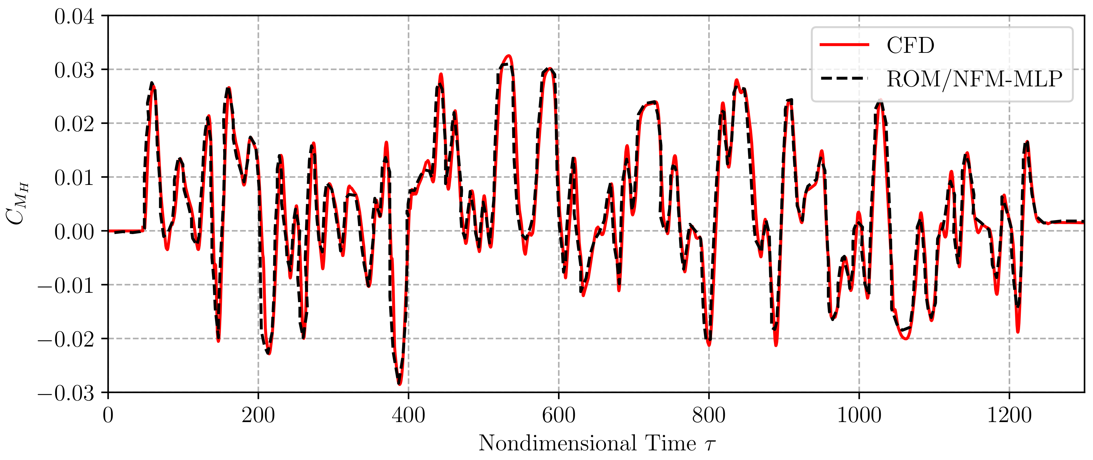
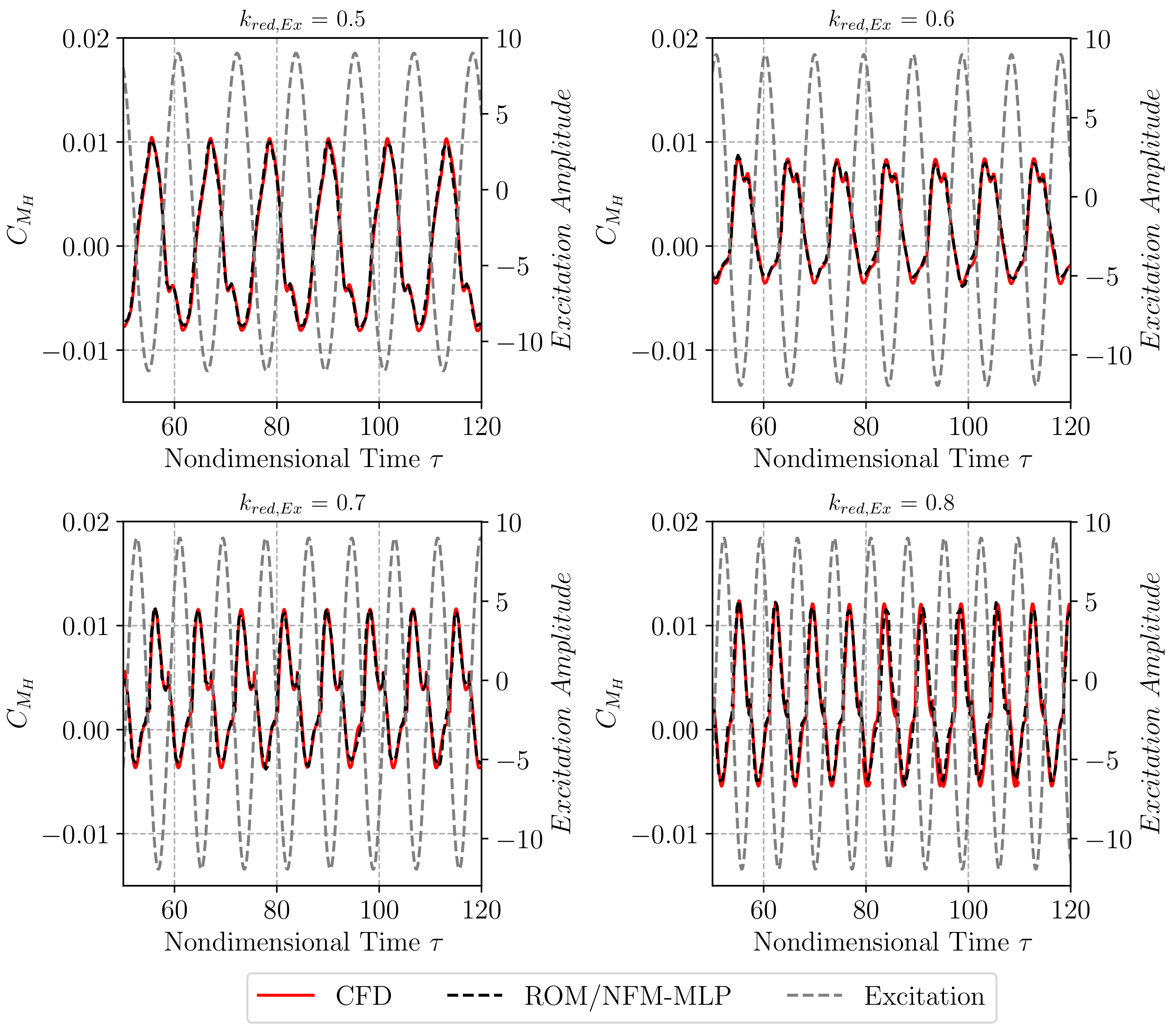
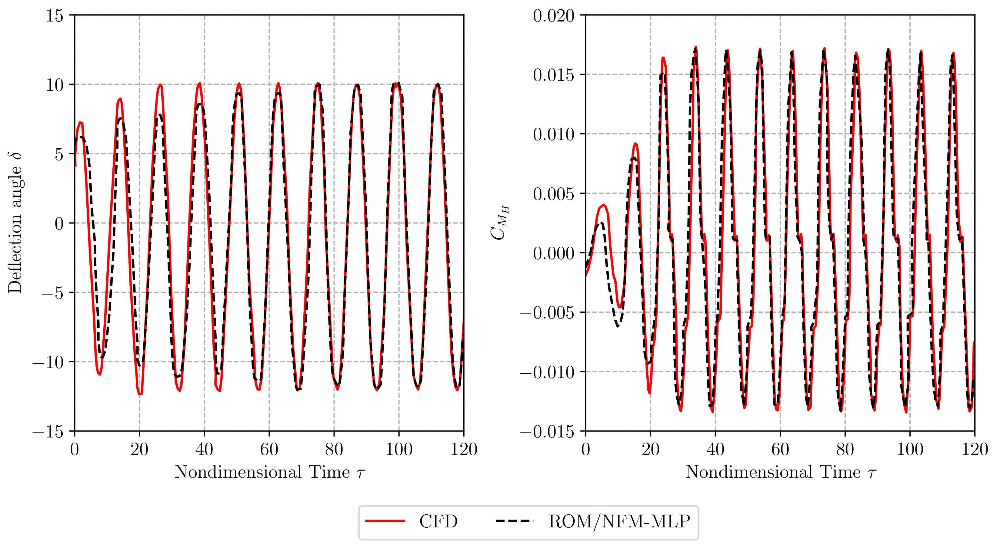
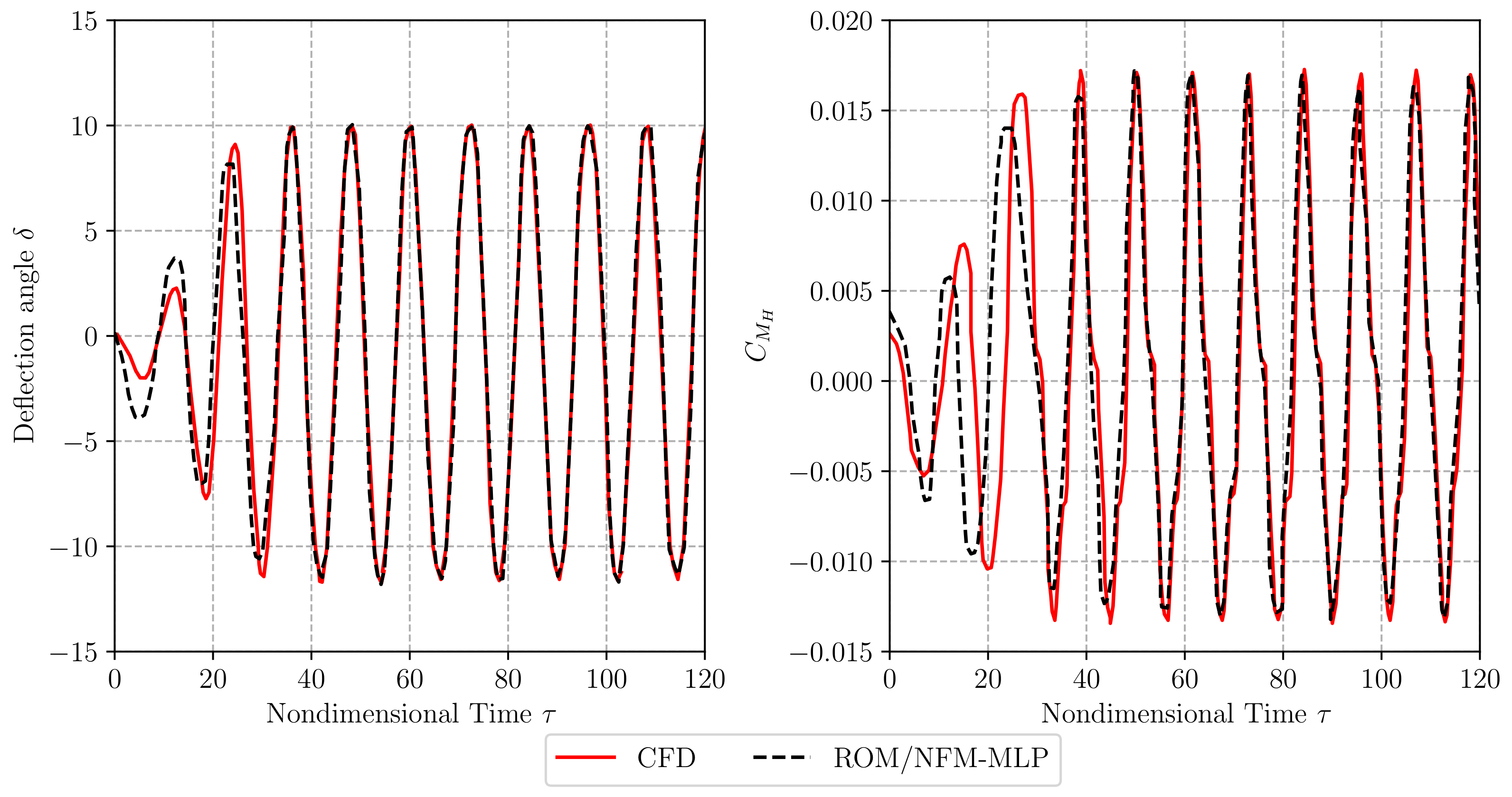
4.2.2. Aeroelastic System Identification
5. Computational Effort
6. Conclusions
Author Contributions
Funding
Acknowledgments
Conflicts of Interest
Nomenclature
| angle of attack, deg | |
| aileron deflection angle, deg | |
| basis function widths of LLM | |
| standard deviation | |
| nondimensional time | |
| fuzzy membership function | |
| angular frequency, 1/s | |
| centers of LLM | |
| hinge moment coefficient | |
| reference chord length, m | |
| F | nonlinear function mapping |
| linear weights of the MLP neural network | |
| nonlinear weights of the MLP neural network | |
| moment of inertia, kgm2 | |
| k | discrete time step |
| k | spring constant |
| , reduced frequency | |
| space extension factor of LLM | |
| m | dynamic delay order of NFM-MLP input vector |
| M | number of neurons of MLP neural network |
| freestream Mach number | |
| hinge moment, N/m | |
| n | dynamic delay order of NFM-MLP output |
| N | number of LLM |
| number of Monte Carlo iterations | |
| number of training samples | |
| q | input of NFM |
| fit factor | |
| Reynolds number | |
| t | time, s |
| start time of deflection, s | |
| freestream velocity, m/s | |
| input vector of MLP | |
| weights of LLM | |
| input vector of NFM | |
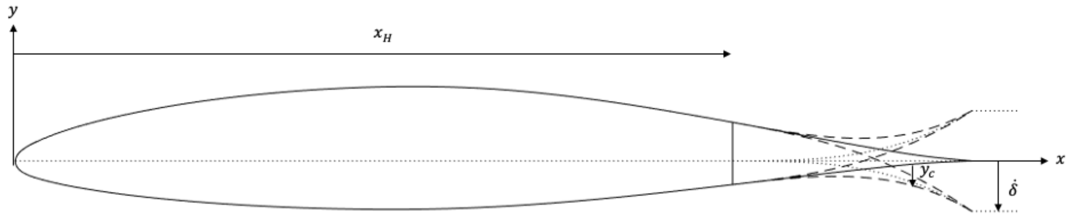
| x | position of points on aileron surface |
| position of hinge point, % | |
| scalar output of the NFM | |
| mean deviation | |
| mean ROM output | |
| scalar output of NFM | |
| camber line |
References
- Lambourne, N.C. Flutter in one degree of freedom. In Manual on Aeroelasticity; Chapter 5; AGARD Report No. 578; AGARD: Neuilly sur Seine, France, 1961. [Google Scholar]
- Bendiksen, O.O. Nonclassical aileron buzz in transonic flow. In Proceedings of the 34th AIAA/ASME/ ASCE/AHS/ASC Structures, Structural Dynamics and Materials Conference, AIAA/ASME Adaptive Structures Forum, AIAA 93-1479, La Jolla, CA, USA, 19–22 April 1993. [Google Scholar]
- Lambourne, N.C. Control-Surface Buzz; Reports and Memoranda 3364; Aeronautical Research Council: London, UK, 1964.
- Steger, J.L.; Bailey, H.E. Calculation of Transonic Aileron Buzz. AIAA J. 1980, 53, 249–255. [Google Scholar] [CrossRef]
- Winter, M.; Breitsamter, C. Reduced-order modeling of transonic buffet aerodynamics. Notes Num. Fluid Mech. 2020, 142, 511–520. [Google Scholar]
- Juang, J.-N.; Pappa, R.S. An eigensystem realization algorithm for modal parameter identification and model reduction. J. Guid. Control Dyn. 1985, 8, 620–627. [Google Scholar] [CrossRef]
- Silva, W.A.; Bartels, R.E. Development of reduced-order models for aeroelastic analysis and flutter prediction using the CFL3Dv6.0 code. J. Fluids Struct. 2004, 19, 729–745. [Google Scholar] [CrossRef]
- Zhang, W.; Ye, Z. Reduced-order-model-based-flutter analysis at high angle of attack. J. Aircr. 2007, 44, 2086–2089. [Google Scholar] [CrossRef]
- Raveh, D.E. Identification of computational-fluid-dynamics based unsteady aerodynamic models for aeroelastic analysis. J. Aircr. 2004, 41, 620–632. [Google Scholar] [CrossRef]
- Hall, K.C.; Thomas, J.; Dowell, E.H. Proper orthogonal decomposition technique for transonic unsteady aerodynamic flows. AIAA J. 2000, 38, 1853–1862. [Google Scholar] [CrossRef]
- Iuliano, E.; Quagliarella, D. Proper orthogonal decomposition, surrogate modeling and evolutionary optimization in aerodynamic design. Comput. Fluids 2013, 84, 327–350. [Google Scholar] [CrossRef]
- Winter, M.; Breitsamter, C. Nonlinear identification via connected neural networks for unsteady aerodynamic analysis. Aerosp. Sci. Technol. 2018, 77, 802–818. [Google Scholar] [CrossRef]
- Zhang, W.; Kou, J.; Wang, Z. Nonlinear Aerodynamic Reduced-Order Model for Limit-Cycle Oscillation and Flutter. AIAA J. 2016, 54, 3304–3311. [Google Scholar] [CrossRef]
- Zhang, W.; Wang, B.; Ye, Z.; Quan, J. Efficient method for limit cycle flutter analysis by nonlinear aerodynamic reduced-order models. AIAA J. 2012, 50, 1019–1028. [Google Scholar] [CrossRef]
- Glaz, B.; Liu, L.; Friedmann, P.P. Reduced-order nonlinear unsteady aerodynamic modeling using a surrogate-based recurrence framework. AIAA J. 2010, 10, 2418–2429. [Google Scholar] [CrossRef]
- Kou, J.; Zhang, W.; Yin, M. Wiener models with a time-delayed nonlinear block and their identification. Nonlinear Dyn. 2016, 85, 2389–2404. [Google Scholar] [CrossRef]
- Mannarino, A.; Mantegazza, P. Nonlinear aeroelastic reduced order modeling by recurrent neural networks. J. Fluids Struct. 2014, 48, 103–121. [Google Scholar] [CrossRef]
- Faller, W.E.; Schreck, S.J.; Luttges, M.W. Neural network prediction and control of three-dimensional unsteady separated flowfields. J. Aircr. 1995, 32, 1213–1220. [Google Scholar] [CrossRef]
- Kou, J.; Zhang, W. Multi-kernel neural networks for nonlinear unsteady aerodynamic reduced-order modeling. Aerosp. Sci. Technol. 2017, 67, 309–326. [Google Scholar] [CrossRef]
- De Paula, N.C.; Marques, F.D.; Silva, W.A. Volterra kernels assessment via time-delay neural networks for nonlinear unsteady aerodynamic loading identification. AIAA J. 2019, 57, 1725–1735. [Google Scholar] [CrossRef] [PubMed]
- Wang, X.; Kou, J.; Zhang, W. Unsteady aerodynamic modeling based on fuzzy scalar radial basis function neural networks. J. Aerosp. Eng. 2019, 233, 5107–5121. [Google Scholar] [CrossRef]
- Tatar, M.; Sabour, M.H. Reduced-order modeling of dynamic stall using neuro-fuzzy inference system and orthogonal functions. Phys. Fluids 2020, 32, 2157–2177. [Google Scholar] [CrossRef]
- Fusi, F.; Guardone, A.; Romanelli, G.; Quaranta, G. Nonlinear reduced order models of unsteady aerodynamics for non-classical aileron buzz analysis. In Proceedings of the International Forum on Aeroelasticity and Structural Dynamics, Bristol, UK, 24–26 June 2013. [Google Scholar]
- Zafar, M.I.; Fusi, F.; Quaranta, G. Multiple input describing function analysis of non-classical aileron buzz. Adv. Aircr. Spacecr. Sci. 2017, 4, 203–218. [Google Scholar] [CrossRef]
- Nelles, O. Nonlinear System Identification—From Classical Approaches to Neural Networks and Fuzzy Models; Springer: Berlin/Heidelberg, Germany, 2011. [Google Scholar]
- Abdessemed, C. Dynamic Mesh Framework for Morphing Wings CFD; University of the West of England: Bristol, UK, 2019. [Google Scholar]
- Erickson, A.L.; Stephenson, J.D. A Suggested Method of Analyzing for Transonic Flutter of Control Surfaces Based on Available Experimental Evidence; NACA-RM-A7F30; NASA: Washington, DC, USA, 1947.
- He, X.; Asada, H. A new method for identifying order of input-output models for nonlinear dynamic systems. In Proceedings of the American Control Conference (ACC), San Francisco, CA, USA, 2–4 June 1993; pp. 2520–2524. [Google Scholar]
- Ljung, L. System Identification: Theory for the User; Prentice Hall: Upper Saddle River, NJ, USA, 1999. [Google Scholar]
- Howlett, J.T. Calculation of Unsteady Transonic Flows with Mild Separation by Viscous-Inviscid Interaction; NASA Technical Paper 3197; Langley Research Center: Langley, BC, Canada, 1992.
- Fusi, F. Numerical Modelling of Non-Classical Aileron Buzz; Politecnico of Milano: Milan, Italy, 2012. [Google Scholar]


| 0.8 | 0.82 | 0.83 | |
| 0.67 | 0.76 | 0.79 |
| 0.5 | 0.6 | 0.7 | 0.8 | |
| () | 91.37% | 92.89% | 92.45% | 91.06% |
| 0.8 | 0.82 | 0.83 | |
| () | 84.37% | 90.89% | 88.47% |
| () | 85.12% | 89.05 % | 88.83% |
Publisher’s Note: MDPI stays neutral with regard to jurisdictional claims in published maps and institutional affiliations. |
© 2020 by the authors. Licensee MDPI, Basel, Switzerland. This article is an open access article distributed under the terms and conditions of the Creative Commons Attribution (CC BY) license (http://creativecommons.org/licenses/by/4.0/).
Share and Cite
Zahn, R.; Breitsamter, C. Neuro-Fuzzy Network-Based Reduced-Order Modeling of Transonic Aileron Buzz. Aerospace 2020, 7, 162. https://doi.org/10.3390/aerospace7110162
Zahn R, Breitsamter C. Neuro-Fuzzy Network-Based Reduced-Order Modeling of Transonic Aileron Buzz. Aerospace. 2020; 7(11):162. https://doi.org/10.3390/aerospace7110162
Chicago/Turabian StyleZahn, Rebecca, and Christian Breitsamter. 2020. "Neuro-Fuzzy Network-Based Reduced-Order Modeling of Transonic Aileron Buzz" Aerospace 7, no. 11: 162. https://doi.org/10.3390/aerospace7110162