1. Introduction
Over the last decade, several robust approaches have been proposed for the control of unmanned aerial vehicles (UAVs), most of which use intelligent and robust control approaches such as fuzzy logic control (FLC), the H∞ technique, sliding mode control (SMC), the backstepping technique, and adaptive control [
1,
2,
3,
4,
5,
6,
7,
8]. The quadrotor is among the most popular UAVs and is widely used in many applications such as surveillance, air mapping, inspection, aerial cinematography, rescue missions, search missions in hostile environments, etc. It presents many desirable features in comparison with other UAVs such as high maneuverability, landing ability, vertical takeoff, and low cost.
The tracking control of quadrotors plays an important role in achieving accurate operations and stable missions. However, realizing the desired objective of control is a very complicated task due to the fact that the quadrotors are underactuated systems that are subject, in general, to undesirable features such as aerodynamic friction force, high nonlinear dynamics, parameter variations, dynamics with strong coupling, gyroscopic uncertain effect, unmodeled dynamics, wind gusts, and other unpredictable and unknown disturbances which affect, in particular, the tracking response and the stability of the control system. To deal with some of these constraints of control, several robust approaches have been developed. In [
3], an adaptive tracking algorithm was developed to force a quadrotor aerial vehicle to achieve a desired task despite modeling errors and disturbance uncertainties. Additionally, in [
9], the authors used both the SMC and terminal SMC to accomplish good tracking control of a small quadrotor UAV despite external disturbances.
SMC is a robust method of control that is well appreciated by many researchers due to its capability to reject the undesirable effects acting on the system dynamics such as uncertainties, unknown disturbances, etc. However, the chattering phenomenon resulting from the fact that the SMC law is discontinuous can be harmful to the actuators [
10]. To eliminate or at least decrease the chattering, higher order SMC (HO-SMC) and boundary layer techniques are usually adopted in the literature to guarantee the desired objective of control [
11,
12,
13,
14,
15]. However, these methods are only employed when the upper bounds of the different kinds of disturbances that influence the control system are known, which constrains their implementation in control systems. In [
16], in order to ensure good tracking control for a small quadrotor UAV, a second-order SMC was developed. Additionally, in [
17], the authors employed a second-order super twisting (SOST) algorithm to ensure the attitude tracking and robustness of a quadrotor against bounded external disturbances. The second-order super-twisting SMC (SOST-SMC) is a particular kind of HO-SMC that has been successfully implemented by several researchers in various fields of systems control [
18,
19,
20]. SOST-SMC was introduced by Levant [
21] in order to handle the chattering problem while simultaneously ensuring the convergence and stability of the control system. However, the SOST-SMC algorithm requires a good estimation of the gains of its control law which is one of its major problems in controlling systems.
On the other hand, due to the fact that fuzzy systems (FSs) are universal approximators [
22], intelligent algorithms using FSs have been extensively employed and successfully applied for the control of uncertain nonlinear systems. In [
23], a FS was used for an autonomous underwater vehicle manipulator to track a desired trajectory in the presence of uncertainties and disturbances. In [
24], the authors used a fuzzy model to describe a wind turbine plant, and as a consequence, a fuzzy controller was designed to achieve the desired task of control. Additionally, in [
25], a proportional integral derivative (PID) controller with a fuzzy logic mechanism was designed for a quadrotor with high nonlinear dynamics and parameter uncertainty. However, type-1 (T1)-FSs (T1-FSs) have a drawback when the linguistic information used to describe the system dynamics contains uncertainties. To cope with this constraint, another kind of FS called type-2 (T2)-FS (T2-FS) was introduced into the modeling and design of robust controllers for complex systems with uncertainties [
26,
27,
28,
29,
30]. The capability of T2-FSs to handle the problem of inaccurate linguistic information much better than T1-FSs is due to the uncertainty property footprint incorporated into the membership functions (MFs) of T2 fuzzy sets [
31,
32,
33].
The main contributions of this paper compared to the previous studies are
- (1)
An intelligent and sophisticated approach to full tracking control is developed for the quadrotor UAVs, subject to the following constraints:
All dynamics of the quadrotor are considered entirely unknown.
No prior knowledge is required for the upper bounds of unknown and unpredictable disturbances acting on the quadrotor dynamics, including aerodynamic perturbations such as unpredictable wind gusts, time varying disturbances, gyroscopic effects, and other unknown disturbances.
The physical parameters of the quadrotor including the mass and the inertia moment are considered entirely unknown and they suffer from time varying disturbances.
- (2)
By taking advantage of the properties of T2-FSs and adaptive control techniques in the design of robust controllers, seven interval T2 adaptive FSs (IT2-AFSs) and five adaptive systems are synthesized to better estimate the unknown dynamics and unknown parameters of the studied quadrotor.
- (3)
A new IT2-adaptive fuzzy reaching sliding mode system (IT2-AFRSMS) is introduced in order to efficiently estimate the optimal values of the gains of a designed reaching sliding mode control law (RSMCL) online. The output of this IT2-AFRSMS is an IT2-adaptive fuzzy RSMCL (IT2-AFRSMCL), designed in such a way as to yield an optimal global control law that is capable of dealing with approximation errors and all unknown and unpredictable disturbances that perturb the quadrotor dynamics, and simultaneously coping with the chattering phenomenon. Then, to tackle the underactuated constraint of the quadrotor control system, two virtual control inputs terms are added to the control system.
- (4)
The parameters of the global developed control law are adjusted online by utilizing the stability analysis theorem of Lyapunov. The proposed algorithm of control is stable in the sense of Lyapunov, and the asymptotic convergence of the system state trajectories is established.
This paper is organized as follows. In
Section 2, the IT2-FSs are described, and then, the problem formulation and the proposed control design for the quadrotor UAVs are presented in
Section 3 and
Section 4, respectively. Finally, in
Section 5, the simulation results for a quadrotor system are presented to show the effectiveness of the designed control algorithm in accomplishing the desired objectives.
2. Interval Type-2 Fuzzy Systems
T2-FSs are used in control systems due to their excellent efficiency when directly handling the measurement uncertainties and inaccurate linguistic information used to synthesize T2 fuzzy rules. Thus, the fuzzy sets for a T2-FS are implemented in such a way that their associated MFs can easily incorporate the above discussed uncertainties through their footprint of uncertainty property. In this study, only IT2-FSs are adopted as approximator systems, on the one hand, because they do not require a lot of computation which makes them more convenient to use in real applications in comparison with other classes of T2-FSs, and on the other hand, due to their efficiency in capturing uncertainties.
The
th IT2 fuzzy rule of an IT2-FS which has
inputs and one output can be formulated as follows [
34]:
where
represents antecedent IT2 fuzzy sets, and
represents consequent IT2 fuzzy sets;
denotes the state vector;
is the output of the system (1); and
denotes the rule number.
In this study, the firing set can be given for the system (1), with the meet operation implemented by the t-norm product, as follows:
where
and
, such that
and
denote, respectively, the left- and right-most values of the MFs associated with the IT2 fuzzy sets
.
Based on the center of sets technique, the outputs of IT2 fuzzy sets of the inference engine are reduced to an IT1 fuzzy set. Then, by adopting the center of gravity method, the crisp output of the system (1) can be given as [
35]
where
and
can be expressed as
where
and
are the lower and upper vectors of fuzzy basis functions, and they are obtained using Karnik–Mandel algorithm [
36], with
;
and
being the left- and right-most conclusion vectors of the system (1) (see [
28] for more details).
3. Model Dynamics of the Quadrotor UAV and Problem Formulation
The quadrotor is a highly nonlinear underactuated system with multiple inputs and multiple outputs and strong dynamic coupling, which is subject to aerodynamic forces, gyroscopic effects, parameter variations, unmodelled dynamics, and unknown and unpredictable disturbances. In order to overcome these constraints, a sophisticated robust tracking control algorithm is developed in this paper for disturbed quadrotor UAVs with unknown dynamics and unknown physical parameters, including the mass and the inertia moment.
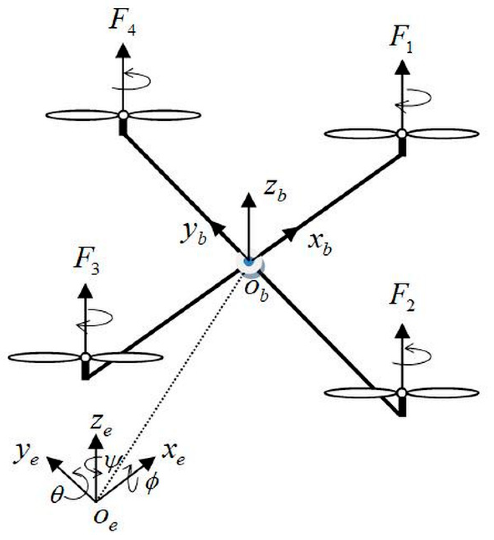
A schematic configuration of a quadrotor UAV system is depicted in
Figure 1, where
denotes an inertial frame and
is a body frame fixed to the quadrotor;
,
and
are, respectively, the roll, the pitch, and the yaw angles, such that
,
, and
.
For more information about the useful structural properties of the quadrotor UAV, see e.g., [
17,
37].
Let and denote the linear and angular velocities in frame , respectively. In addition, let and denote the Euler angles and the position of the quadrotor in frame , respectively.
The relation between the velocities (
,
) and (
,
) can be expressed as follows:
where
and
.
Using the Newton–Euler formulation, the model describing the quadrotor UAV dynamics can be given as follows:
where
,
and
denote, respectively, the inertia parameters along the
,
, and
axes;
,
and
denote the quadrotor’s position in the earth-fixed frame
;
(
) are the bounded unknown disturbances including gyroscopic effects, time varying disturbances, aerodynamic perturbations such as unpredictable wind gusts, and other neglected and unmodeled dynamics;
is the gravity acceleration;
,
, and
denote theair drag coefficients along the
,
, and
directions, respectively;
is the mass of the quadrotor;
and
; and
(
) are the control inputs of the system (6), and they are defined as follows:
where
is the distance between the center of mass and the center of each rotor of the quadrotor;
and
are the thrust factor and the drag factor, respectively;
(
) is the force generated by the rotor
; and
(
) denotes the angular velocity of the
th rotor.
The state vector is defined to be
and assumed to be available for measurement, with
being the first element of the state vector. Then, system (6) can be reformulated as:
where
and
;
and
are, respectively, the
th output and the
th input of system (8), where
and
are virtual control inputs to be designed later.
In this study, and are unknown nonlinear continuous functions. In addition, it is assumed that the system (8) is controllable. So, we consider that exists.
4. Control Law Design
The main objective of control is to steer state to a desired reference .
As the system (8) describes a quadrotor UAV with unknown dynamics that is subject to unknown and unpredictable disturbances, a new robust IT2-AFRSMS was designed to deal with such constraints while ensuring the best tracking performance and avoiding the chattering phenomenon.
The system (8) has four independent inputs to control its six outputs; it is an underactuated system. Therefore, in order to overcome this constraint, two virtual control inputs, and , are introduced to generate the desired and angles to achieve the desired longitudinal and lateral position tracking.
The desired
and
angles are determined according to the following equation:
After some rearrangement, we get
In order to better estimate the unknown nonlinear functions of the system (8), the IT2-FS defined in (3) is used to substitute
and
with their IT2-AFS approximators
and
, respectively, as given in the following equation:
where
and
such that
,
,
and
are, as described in (4), the vectors of fuzzy basis functions;
and
are adaptive parameter vectors; and
and
denote the number of fuzzy rules of the IT2-AFSs
and
, respectively.
In order to estimate the rest of the unknown terms
(
), the following adaptive systems are designed as
where
,
are adaptive parameters.
4.1. Sliding Mode Control Law Design
The SMC is considered to be among the most robust methods of control and is capable of steering the system state trajectories towards the desired dynamics.
Let
be the tracking error. Then, the sliding surface can be defined as [
38]
where
is a matrix of diagonal slopes
(
), and
denotes the system order.
The quadrotor (8) is a second-order system (
). Therefore, Equation (13) becomes
Considering the system defined in (8), the time derivative of the sliding surface can be obtained as
The desired dynamics are obtained when the following condition is verified: .
The optimal parameters of
and
can be expressed as
The minimum approximation error of
and
is then given by
where
and
are the optimal approximations of
and
, respectively, with
.
The control law synthesized to satisfy the desired objective of control is expressed as
where
is a RSMCL.
The RSMCL
is introduced in order to maintain the desired dynamics (
) by ensuring that the effects of the approximation errors and all disturbances that affect the quadrotor dynamics are eliminated or at least reduced. Therefore, to guarantee the sliding mode, the expression of
is given as
where
, with
, and
to make sure that the
function is continuous everywhere;
,
, and
are positive reaching control gains;
is the convergence time of the sliding surface
to a vicinity
of
.
The adaptation laws of the IT2-AFSs defined in (11) and the adaptive systems given by (12) are expressed as
where
and
are positive learning parameters.
Theorem 1. Using the IT2-FS approximators defined in (11), the adaptive systems presented in (12) and the adaptation laws expressed in (20), the control law (18) developed for the underactuated quadrotor (8) is stable in the sense of Lyapunov and the asymptotic convergence of the tracking error is established despite unknown dynamics, unknown physical parameters, and all unknown and unpredictable disturbances that affect the control system.
Proof 1. Use the following augmented Lyapunov function candidate:
where
;
, such that
,
;
The time derivative of the above equation is
where
.
Substituting (23) into (22) gives
where
such that
and
;
, with
; and
.
Substituting (20) into (24) gives
Substituting
by its expression gives
Consider the following inequality:
If the following condition is assured:
Then the inequality (27) is verified, and therefore, the functions defined in (26) are negative. Thus, Proof 1 is established. □
In order to ensure the above inequality (28), the values of parameters , , and should be well chosen. However, in practice, choosing the right values of these parameters, which ensures the desired tracking objective while simultaneously avoiding the chattering, remains one of the major problems in systems control. The large values generate a large amount of chattering, and the small ones affect the robustness of the controlled system against uncertainties and disturbances and deteriorate the performance of the tracking control. Therefore, in order to overcome this control constraint, in this study, we propose the introduction of a rigorous IT2-AFRSMS in order to efficiently estimate the optimal values of parameters , and online to ensure both the desired performance of tracking control of the quadrotor (8) by guaranteeing the condition shown in (28), and avoiding the chattering phenomenon.
4.2. Proposed Adaptive Fuzzy Sliding Mode Control Design Method
In order to efficiently estimate the optimal gains of the RSMCL defined in (19), a new IT2-AFRSMS similar to the IT2-FS defined in (3) and characterized by the following properties is introduced:
The sliding surface is the input vector of the IT2-AFRSMS;
The outputs of the IT2-AFRSMS are the online estimations of the terms , , and of the RSMCL .
Thus,
,
and
are substituted, respectively, by their IT2-AFS estimators, as follows:
where
,
and
are, as described in (4), the vectors of fuzzy basis functions;
,
and
are the online adjustable parameter vectors;
is the number of rules.
We define the optimal parameters of the IT2-AFSs
,
, and
as
The global proposed control law is designed as follows:
where
is the designed IT2-AFRSMCL.
The adaptation laws designed for the estimators defined in (29) are given as:
where
,
and
are positive learning parameters.
Theorem 2. Using the IT2-AFSs defined in (11) and (29), the adaptive systems defined in (12), the adaptation laws given by (20) and (32), the global control law (31) developed for the underactuated quadrotor (8) is stable in the sense of Lyapunov, and the asymptotic convergence of the tracking error is established despite the unknown dynamics, unknown physical parameters, and all of the unknown and unpredictable disturbances that affect quadrotor dynamics.
Proof 2. Use the following new augmented Lyapunov function candidate:
where
,
,
.
Considering Equations (21), (25), and (31), the time derivative of (33) gives:
Let
,
, and
be, respectively, the online optimal estimations of
,
and
that ensure the best tracking control performance of the quadrotor (8) by providing optimal gains in
,
, and
for the RSMCL
, which allows the perturbations
to be efficaciously rejected through verification of the condition shown in (28) while simultaneously avoiding the undesired chattering. Then, by introducing the optimal IT2-AFRSMCL
into (34), we get:
Substituting
,
, and
by their expressions defined in (32) gives
If the following inequality is guaranteed,
Then, the values of defined in (36) are negative.
Additionally, since , , and are the online optimal estimations of , , and that ensure the condition shown in (28) is satisfied while simultaneously avoiding chattering. Thus, the condition shown in (37) is verified. Therefore, Proof 2 is established. □
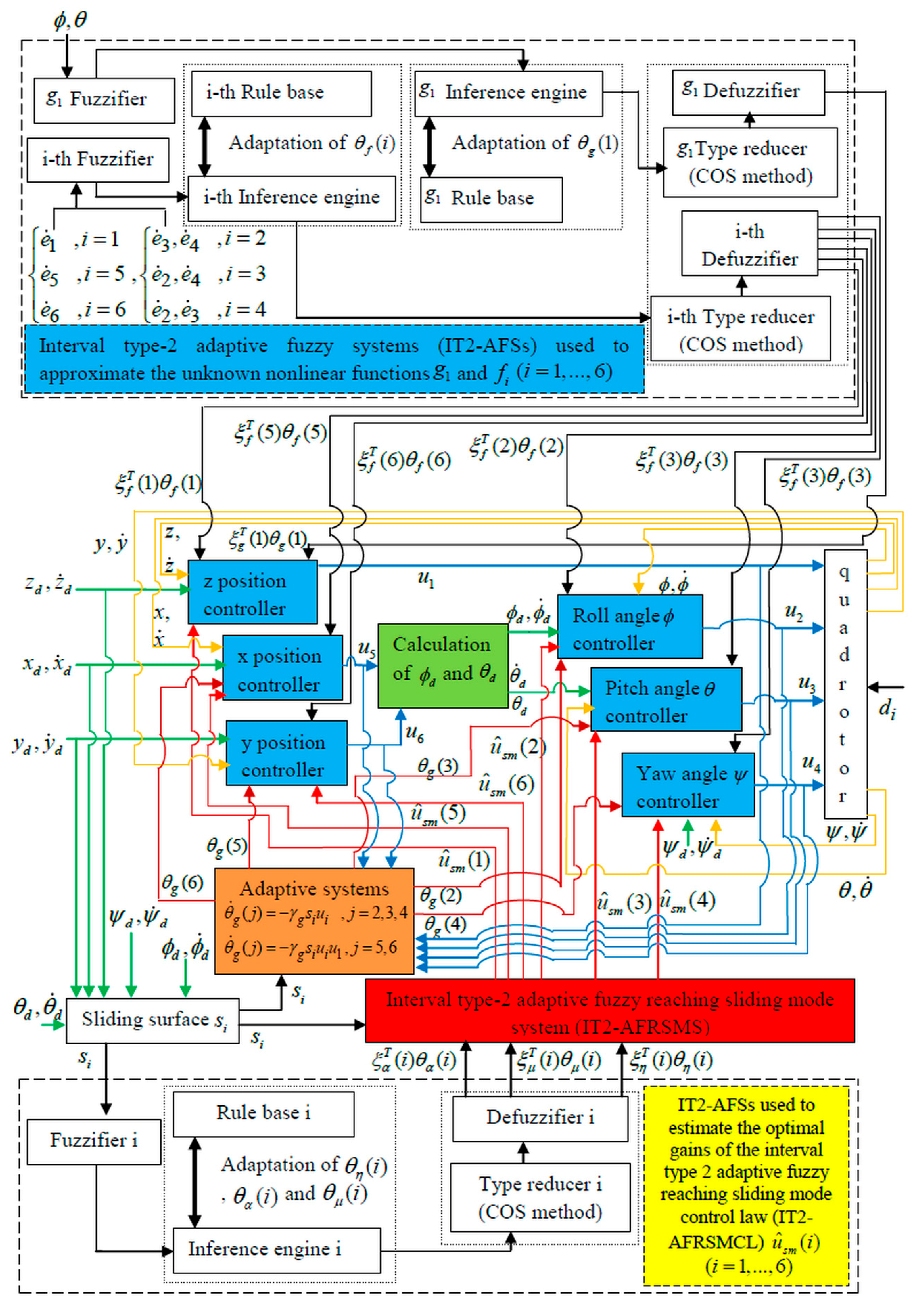
The control design method developed in this paper is represented in
Figure 2.
5. Simulation Results
In order to validate the effectiveness of the developed tracking control method for the quadrotor system (8), we present the simulation results in this section.
The quadrotor parameters used for simulation are listed in
Table 1 below.
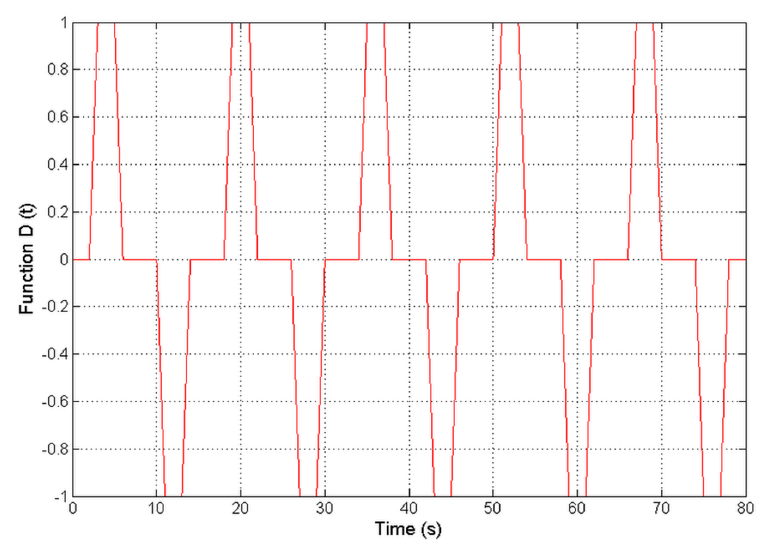
All unknown disturbances that affect the quadrotor system (8), including gyroscopic effects and aerodynamic perturbations, are represented by
With the function
being represented in
Figure 3 below.
The mass and the inertia moment of the quadrotor (8) are unknown and present the following time varying disturbances:
The main objective of control is to steer the state to the desired reference, . The angles and are determined according to Equation (10).
Since the studied quadrotor (8) has unknown dynamics and unknown physical parameters and because it is subject to unknown and unpredictable disturbances and suffers from time varying perturbations, we can use the developed control law (31) to obtain the intended objectives of control.
The initial positions and angle values are .
The sliding surfaces are set to , , , , , and , such that , , , , , and are the tracking errors.
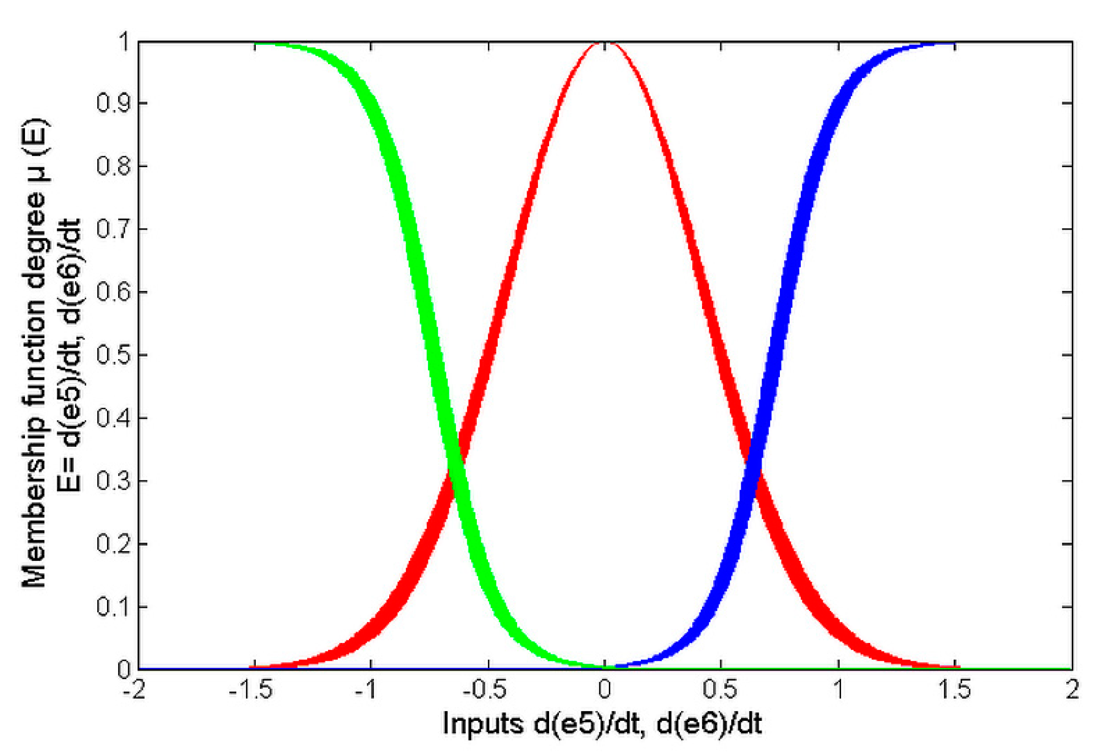
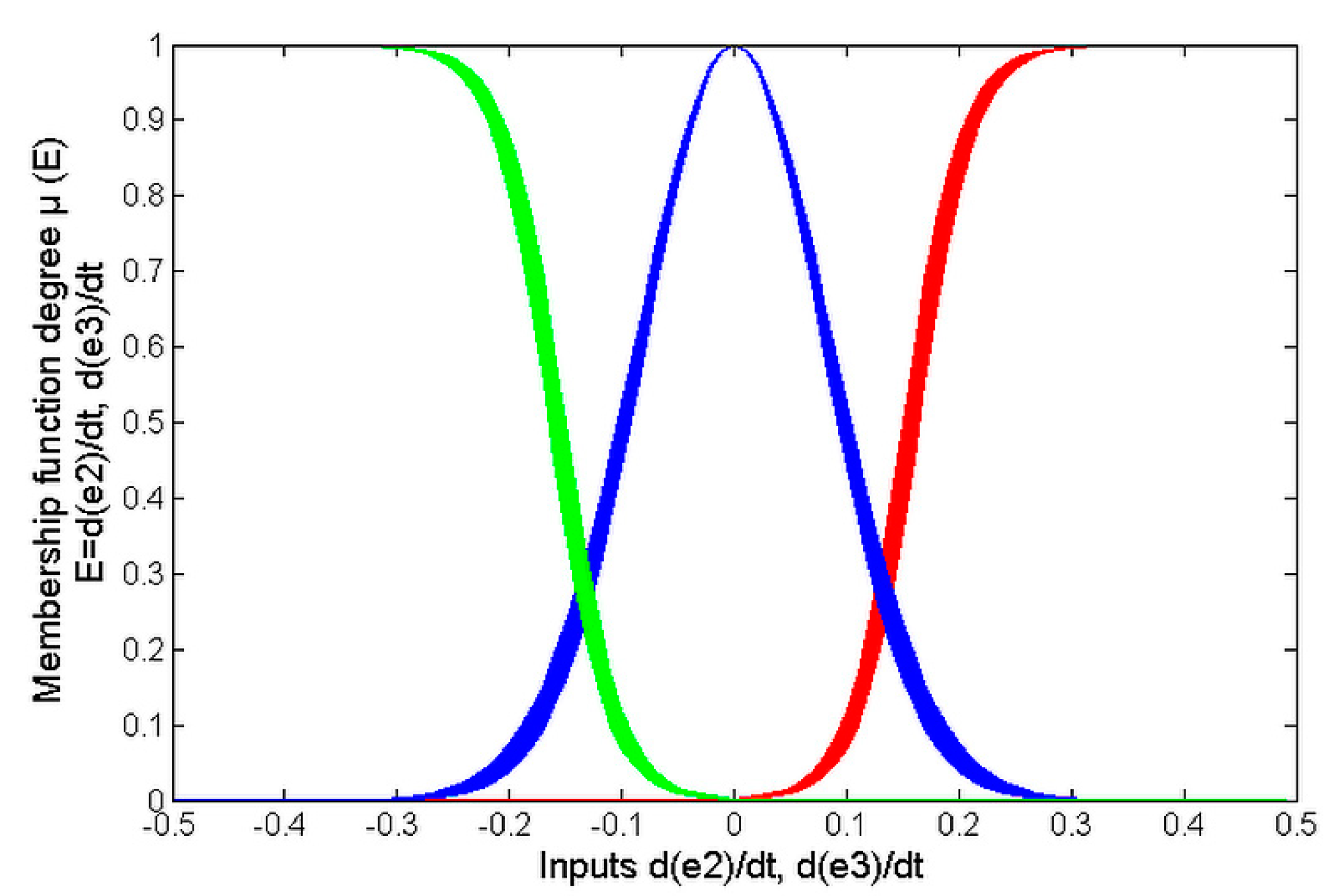
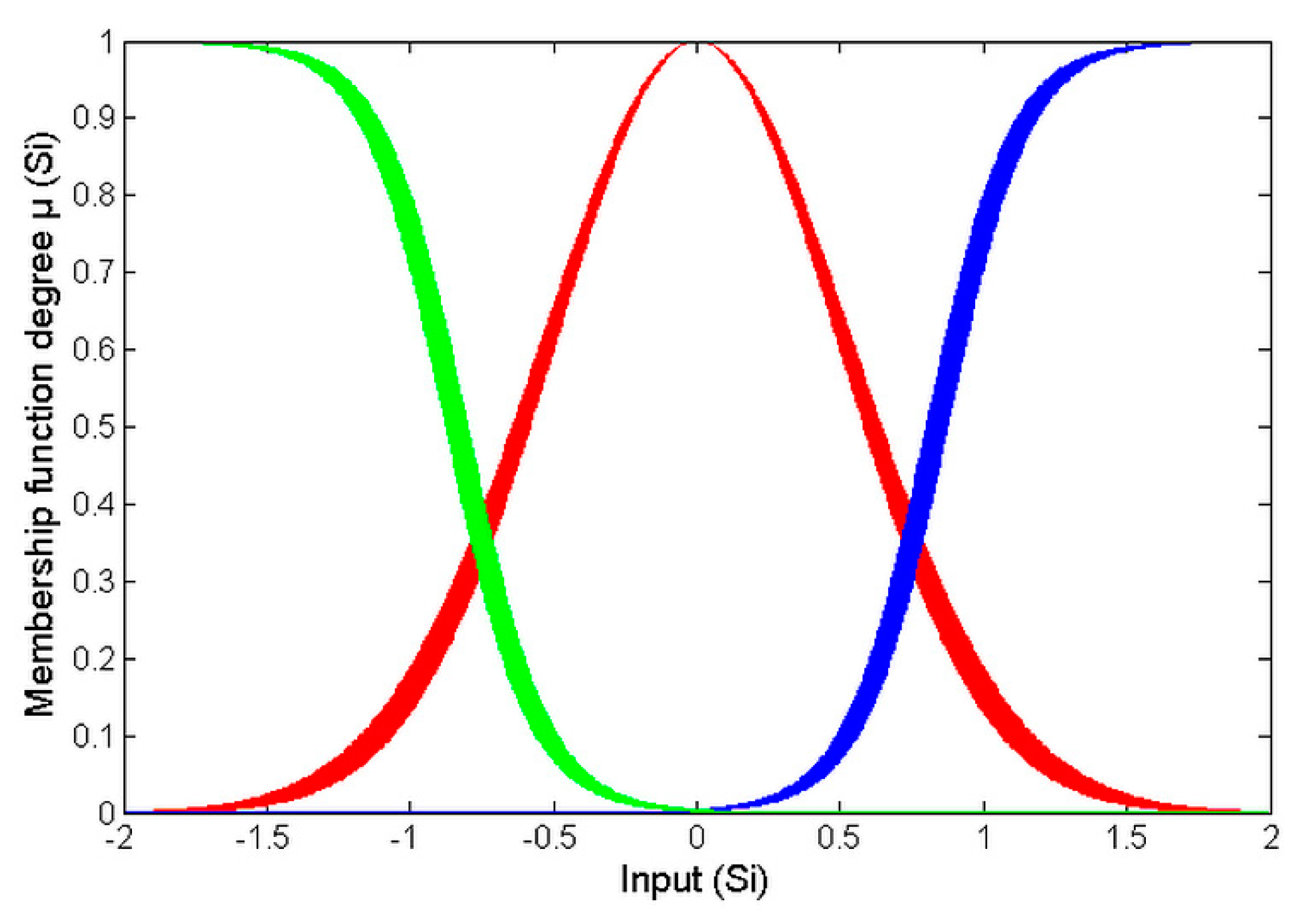
It is assumed that and belong to and belongs to .
The IT2-AFSs
,
and
have, respectively, the inputs
,
and
;
has two inputs,
and
;
has two inputs,
and
; and
has two inputs,
and
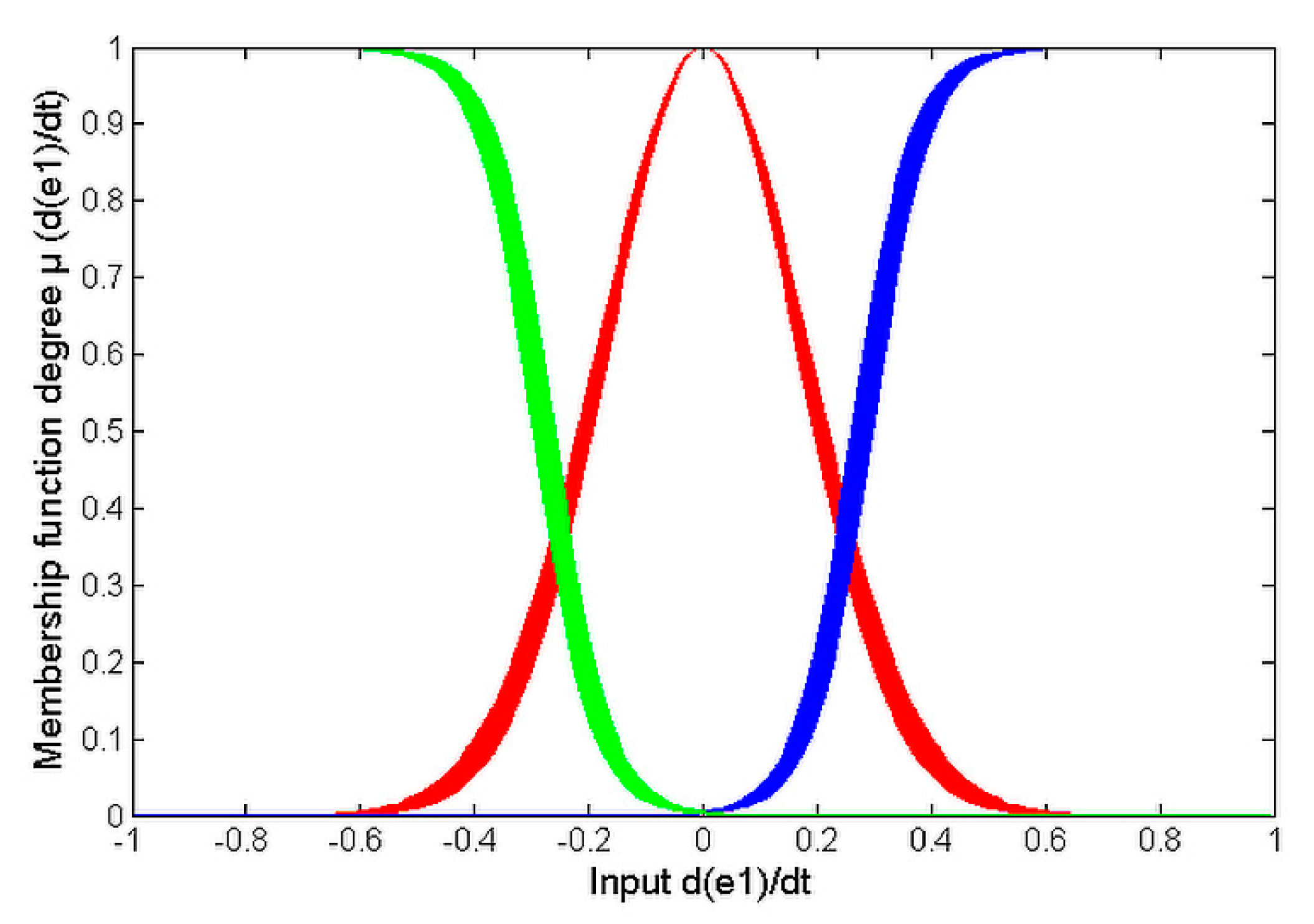
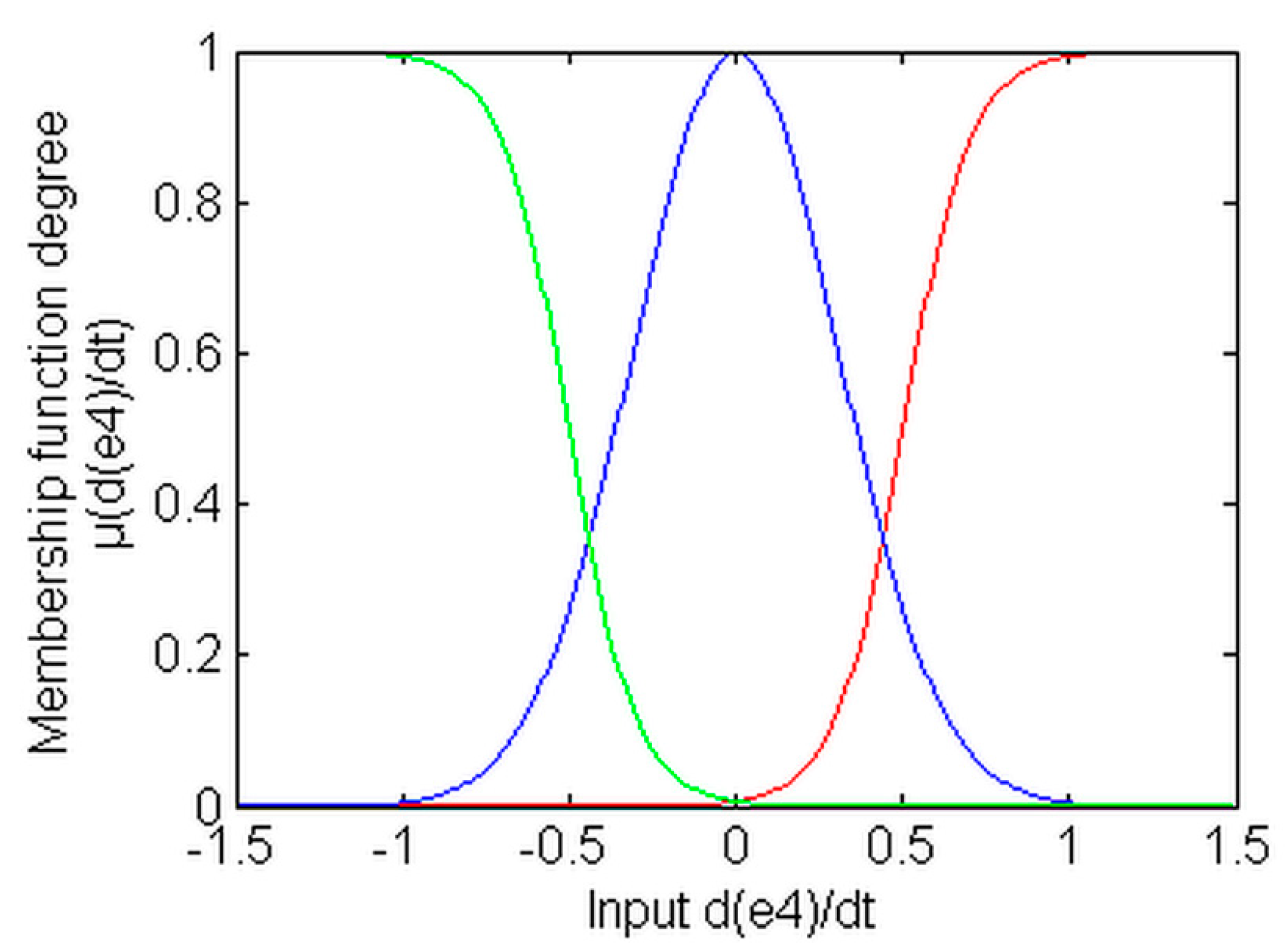
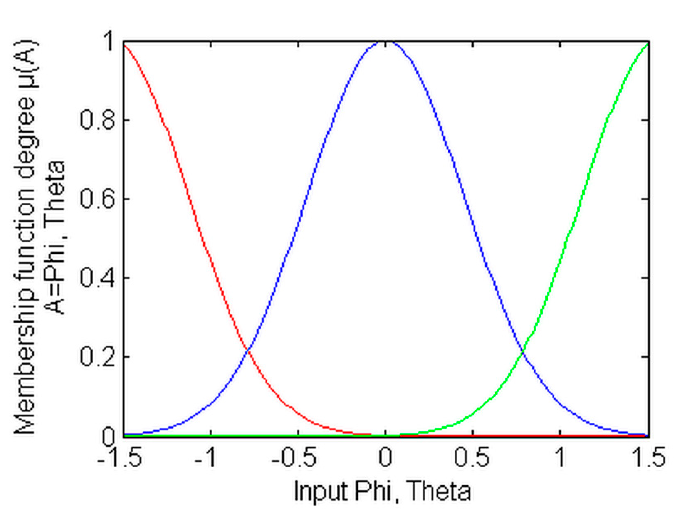
. All of these inputs are defined by three MFs, as depicted in
Figure 4,
Figure 5,
Figure 6 and
Figure 7.
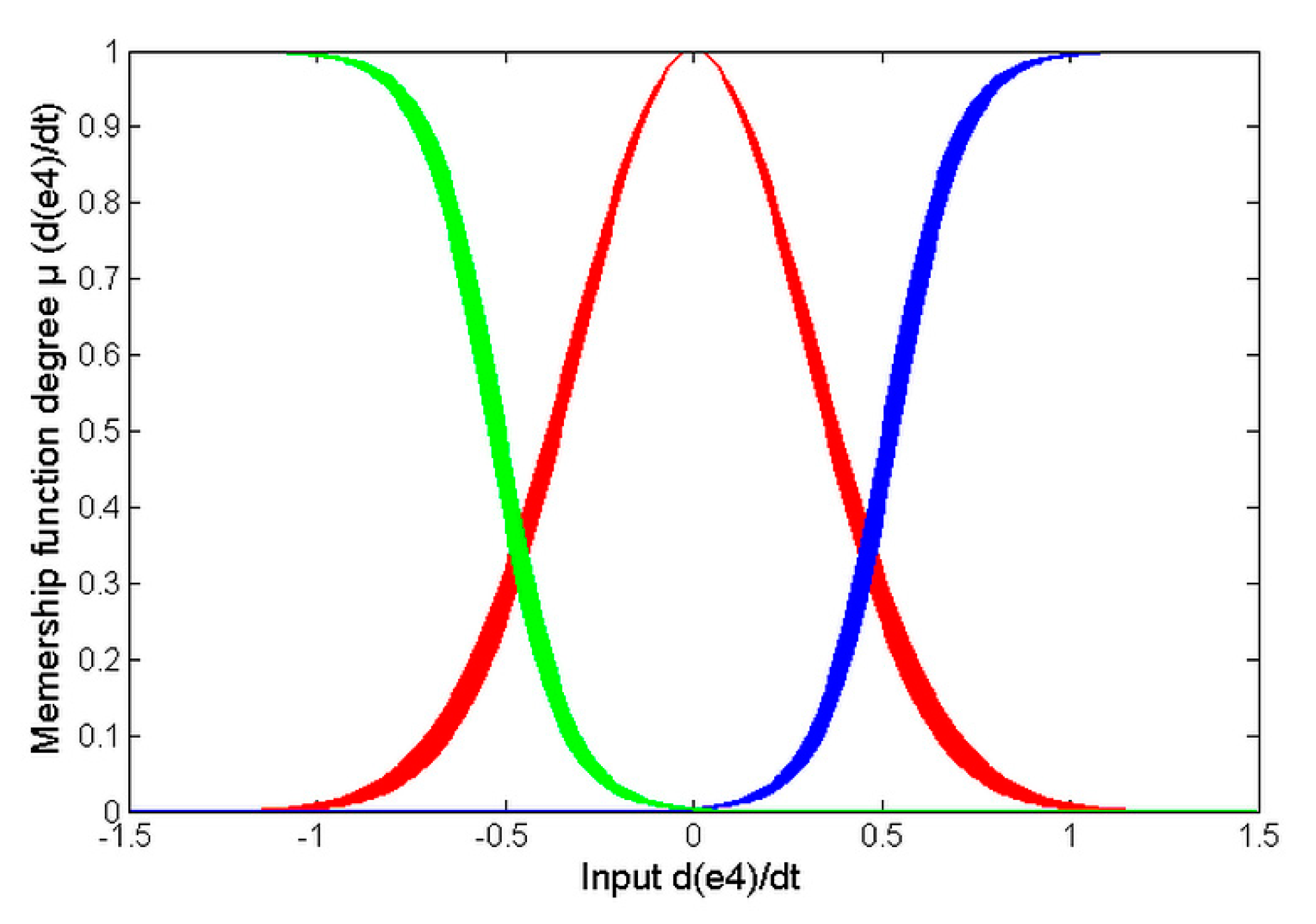
The MFs designed for
are depicted in
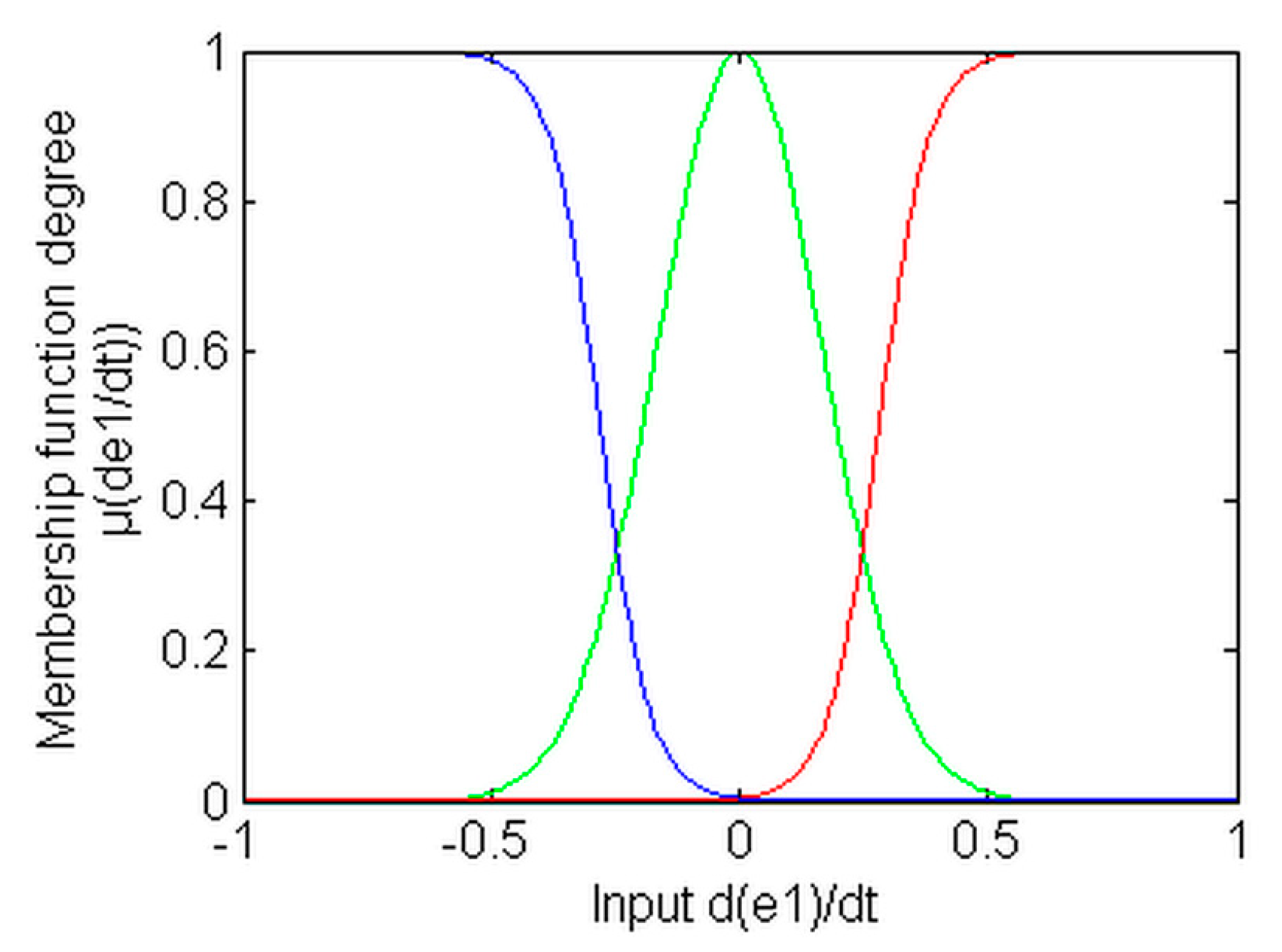
Figure 4; the MFs used by
and
are represented in
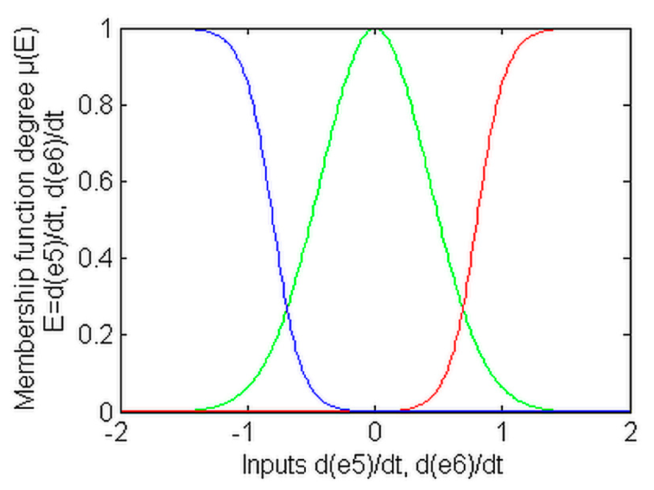
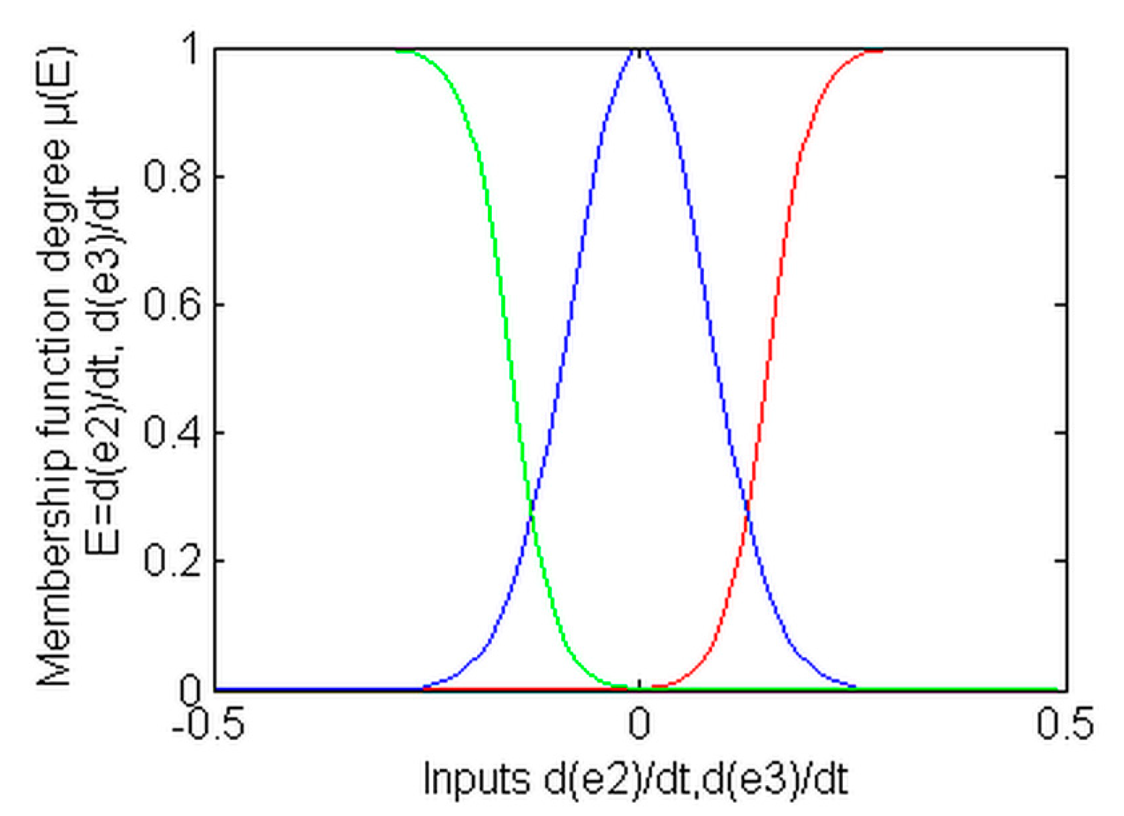
Figure 5; the MFs used for the inputs
and
are shown in
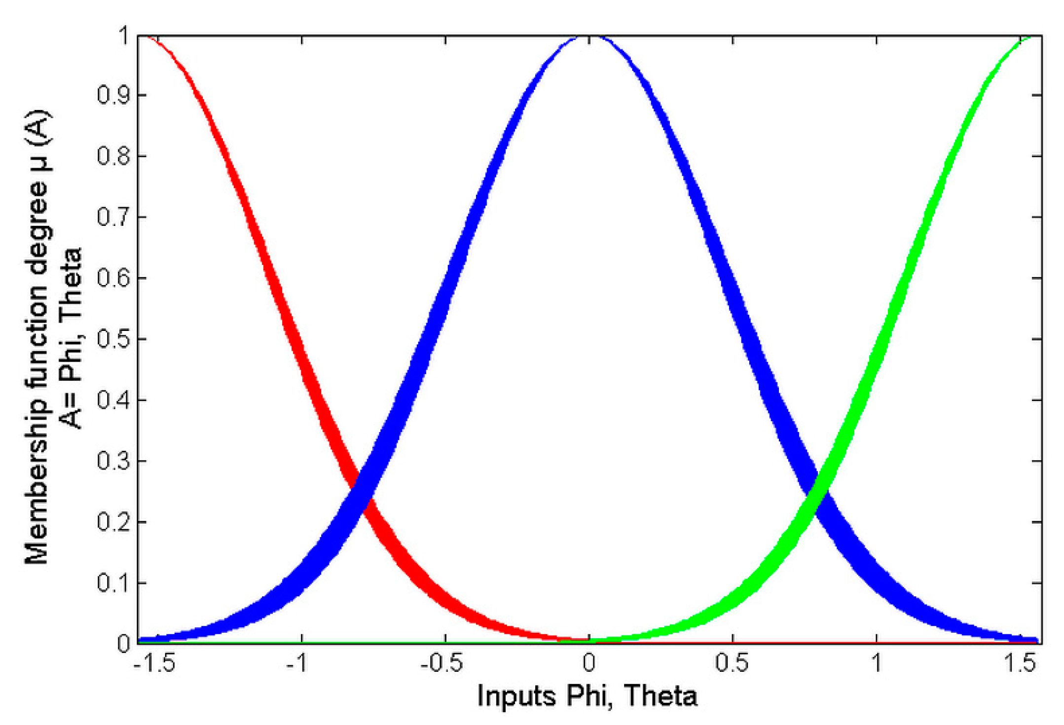
Figure 6; and the MFs designed for
are depicted in
Figure 7.
On the other hand, the IT2-AFS
has two inputs,
and
. Then, three MFs are used for each input of
, as shown in
Figure 8.
The MFs used by the IT2-AFRSMCL
, (
) are represented in
Figure 9 below.
In order to confirm the effectiveness of the proposed tracking control method (PTCM), a comparison was carried out with its counterpart method that uses T1-AFSs instead of T2-AFSs and uses a SOST-SMC to reject the undesired effects caused by unknown disturbances and approximation errors. Henceforward, the abbreviation CMTC refers to this method of tracking control.
The control law used by CMTC is given by Equation (38):
where
and
are T1-AFSs, and
are adaptive systems and they are designed in the same way as those defined in (12),
, such that
and
denote the gains of the reaching SOST control term
.
The constant parameters of the two compared tracking control approaches are given in
Table 2.
The simulation results obtained from the comparison that was carried out between the two approaches of control are illustrated in
Figure 15,
Figure 16,
Figure 17,
Figure 18,
Figure 19,
Figure 20,
Figure 21,
Figure 22,
Figure 23,
Figure 24,
Figure 25,
Figure 26,
Figure 27 and
Figure 28.
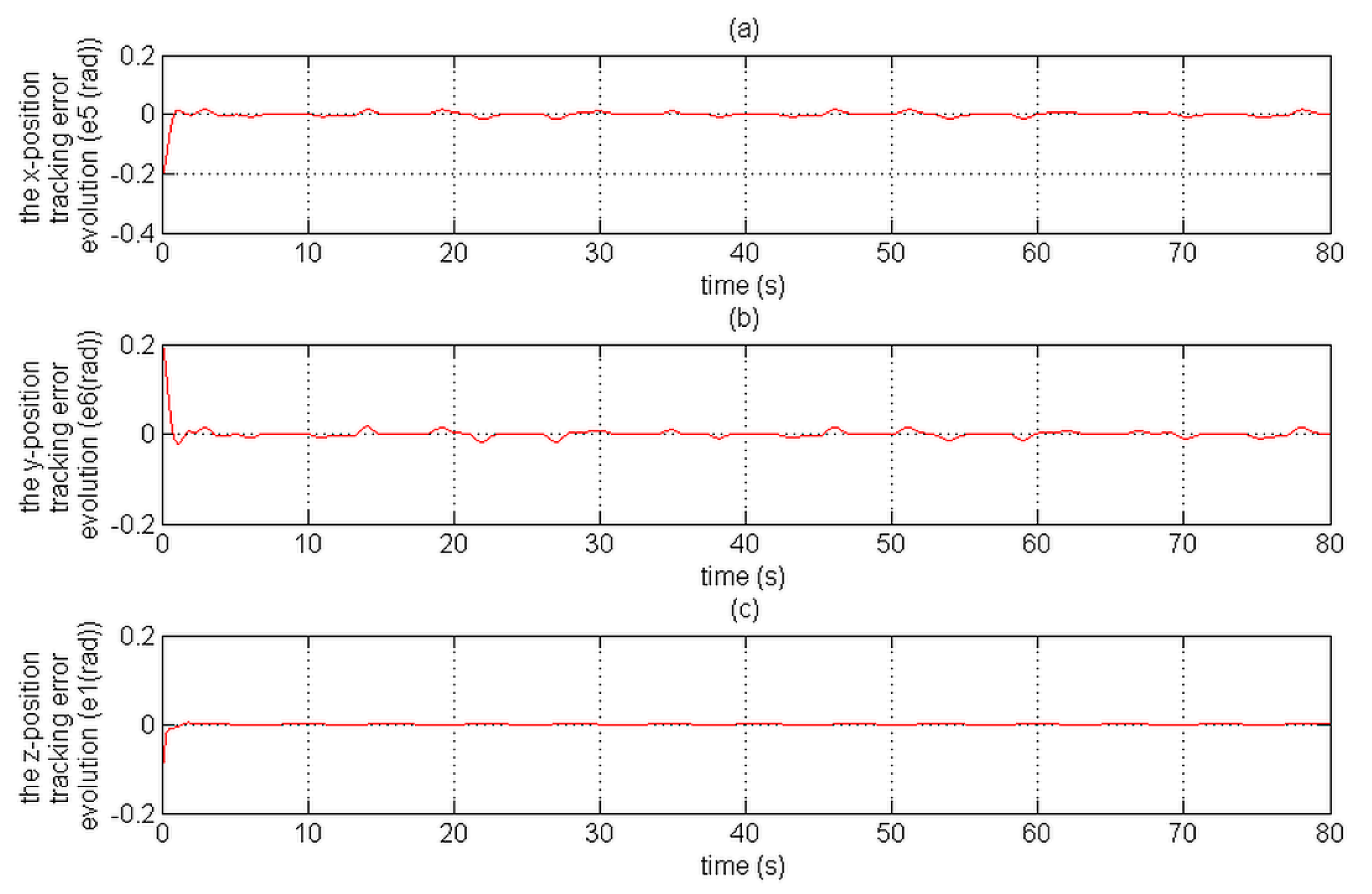
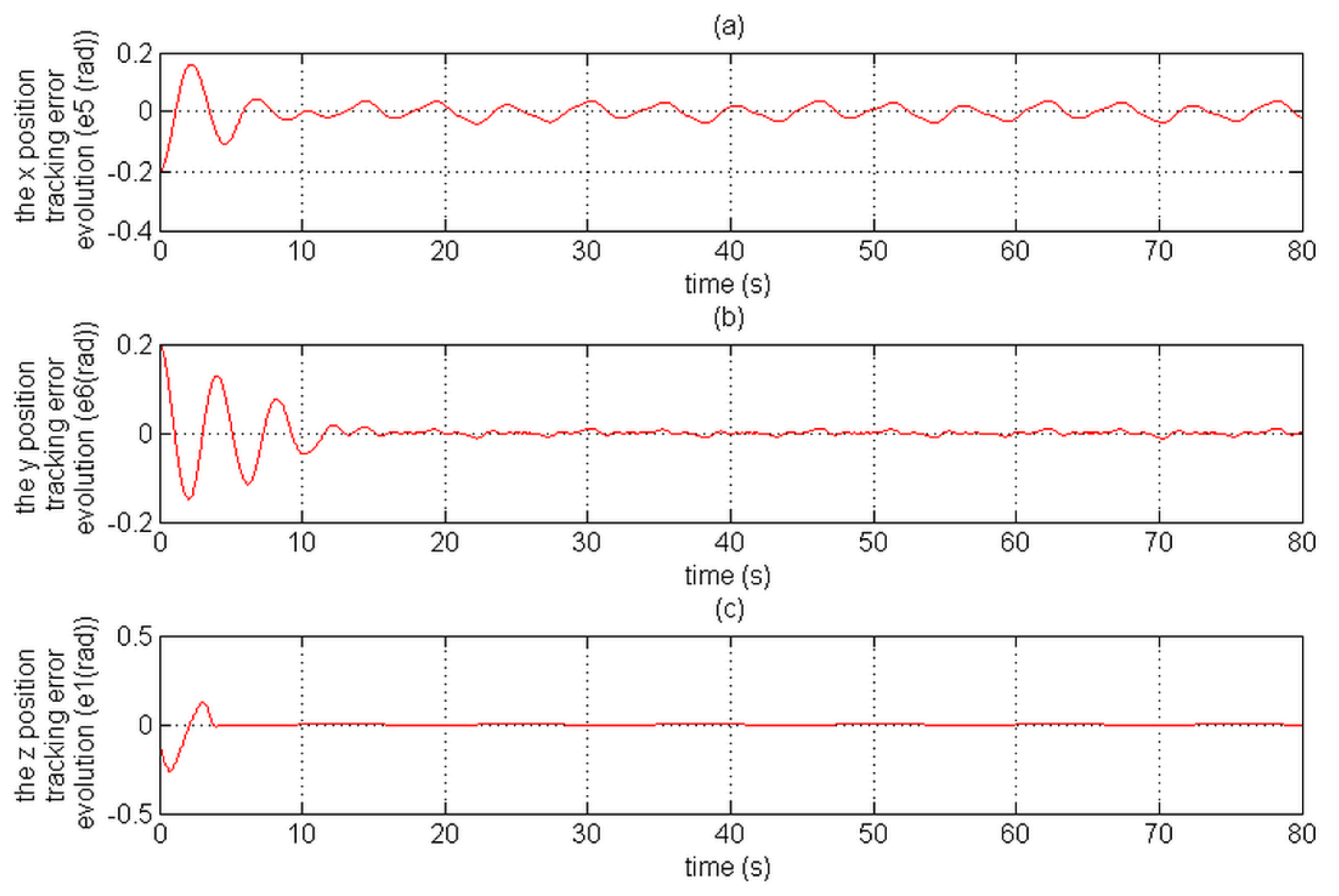
Figure 15 and
Figure 16 depict the position tracking errors;
Figure 17 and
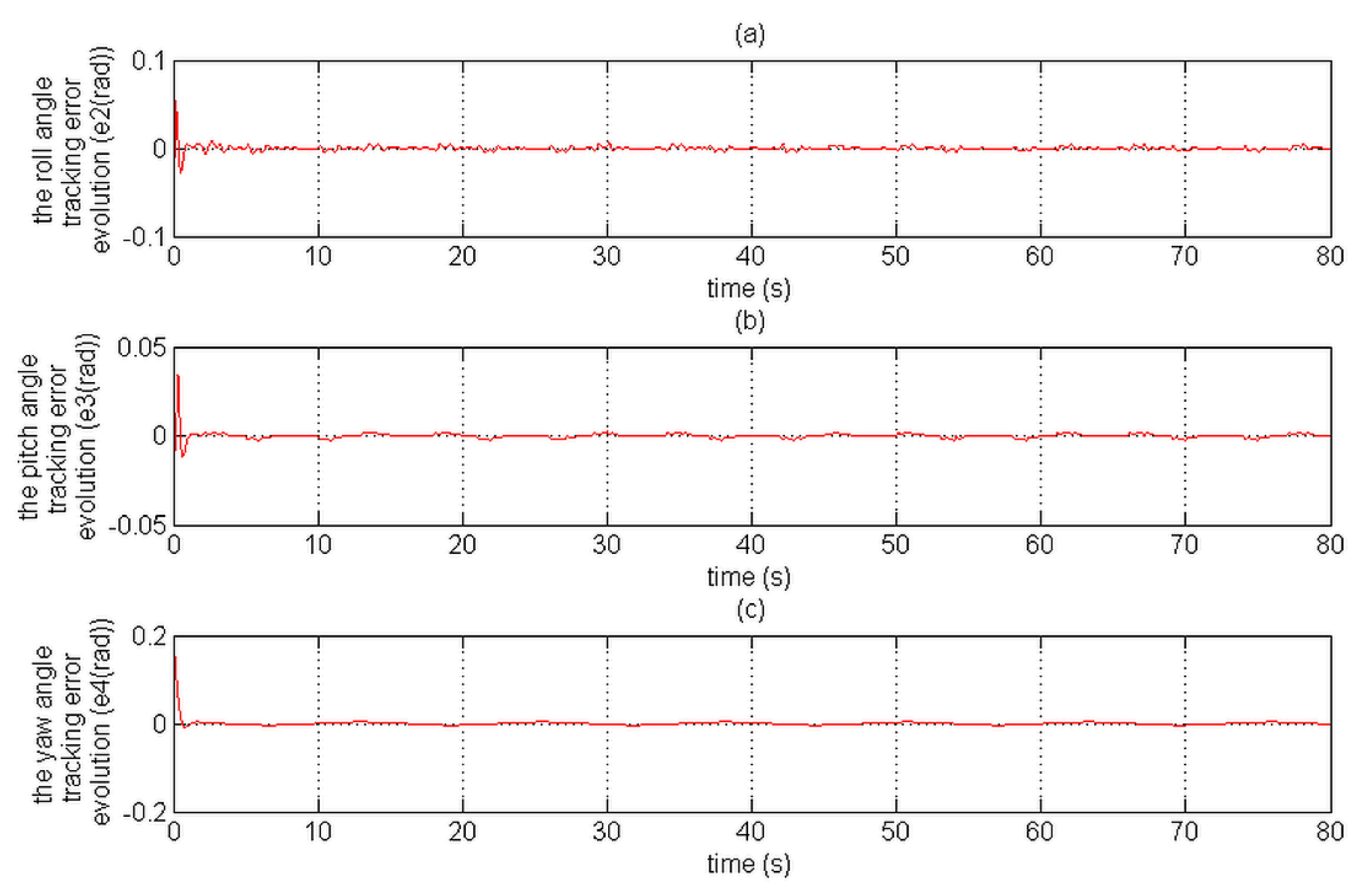
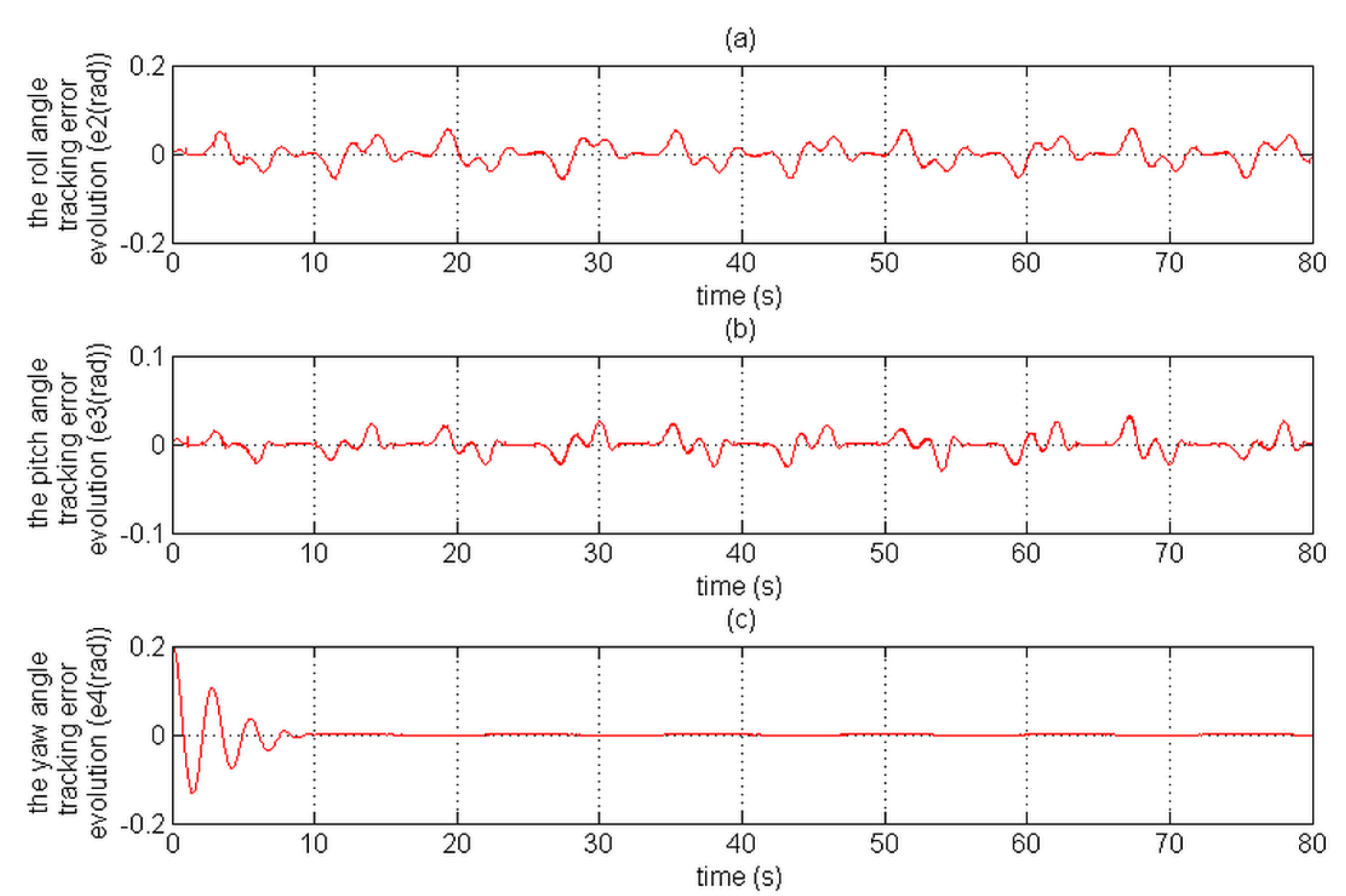
Figure 18 represent the attitude tracking errors;
Figure 19 and
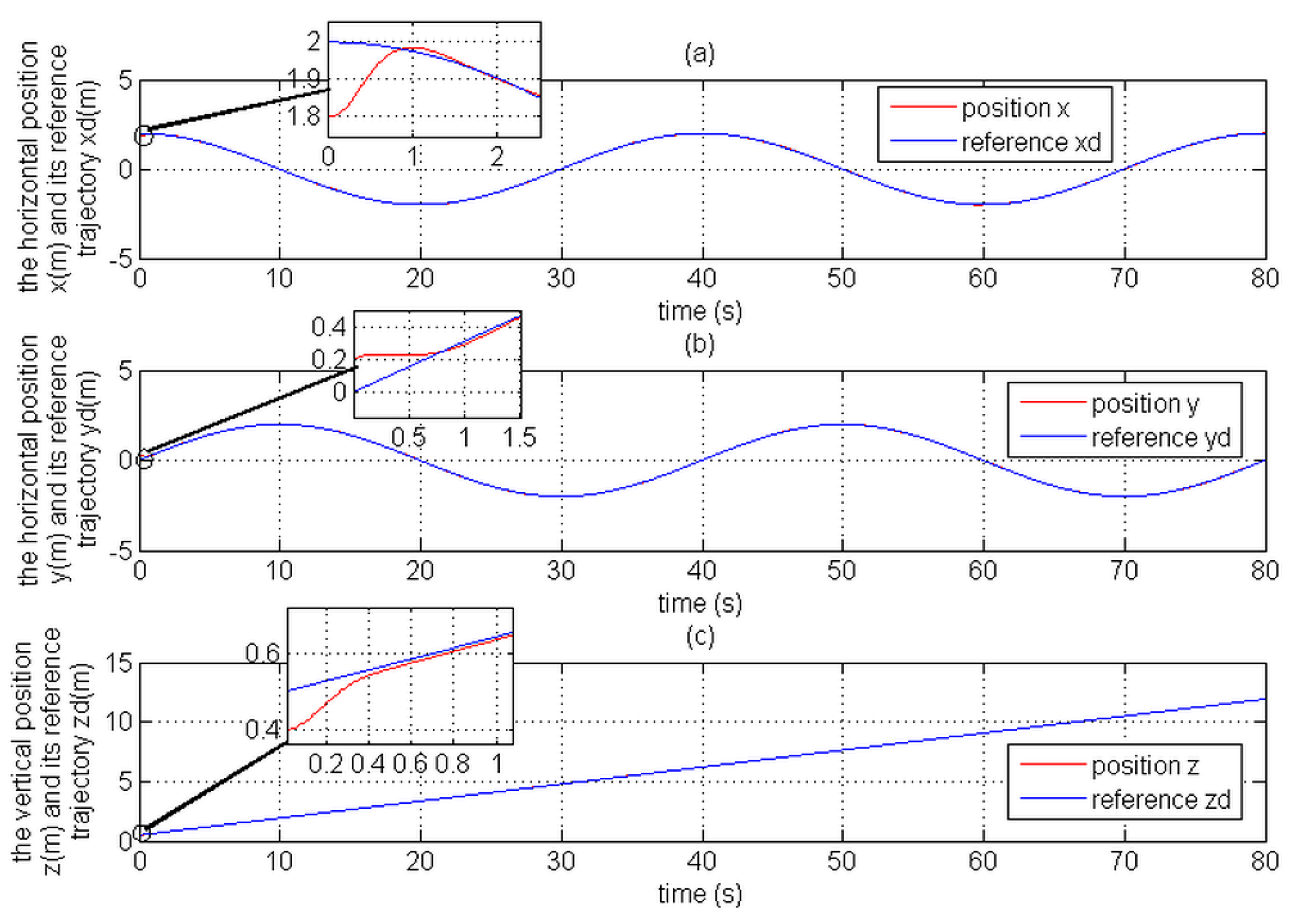
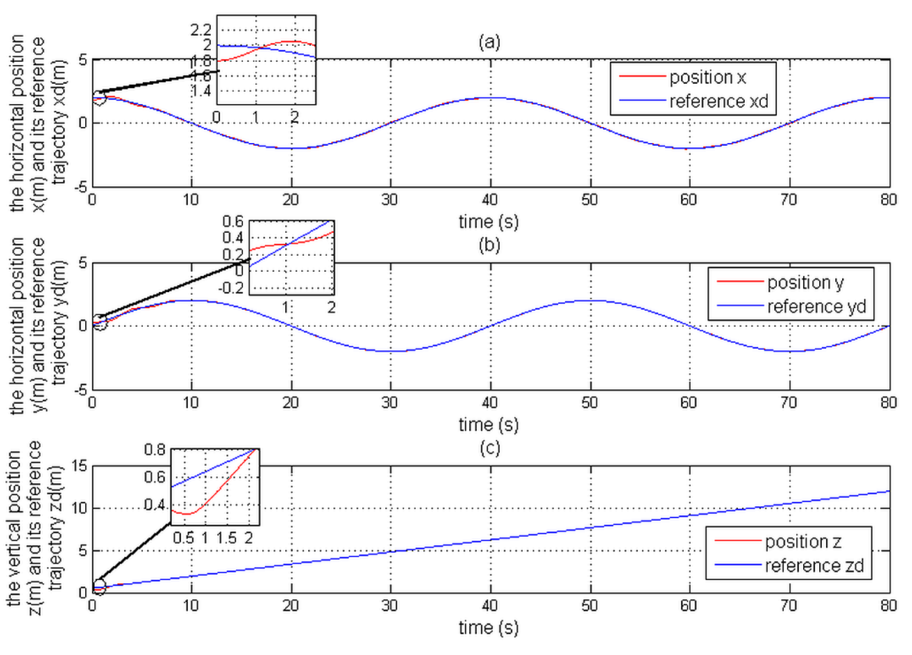
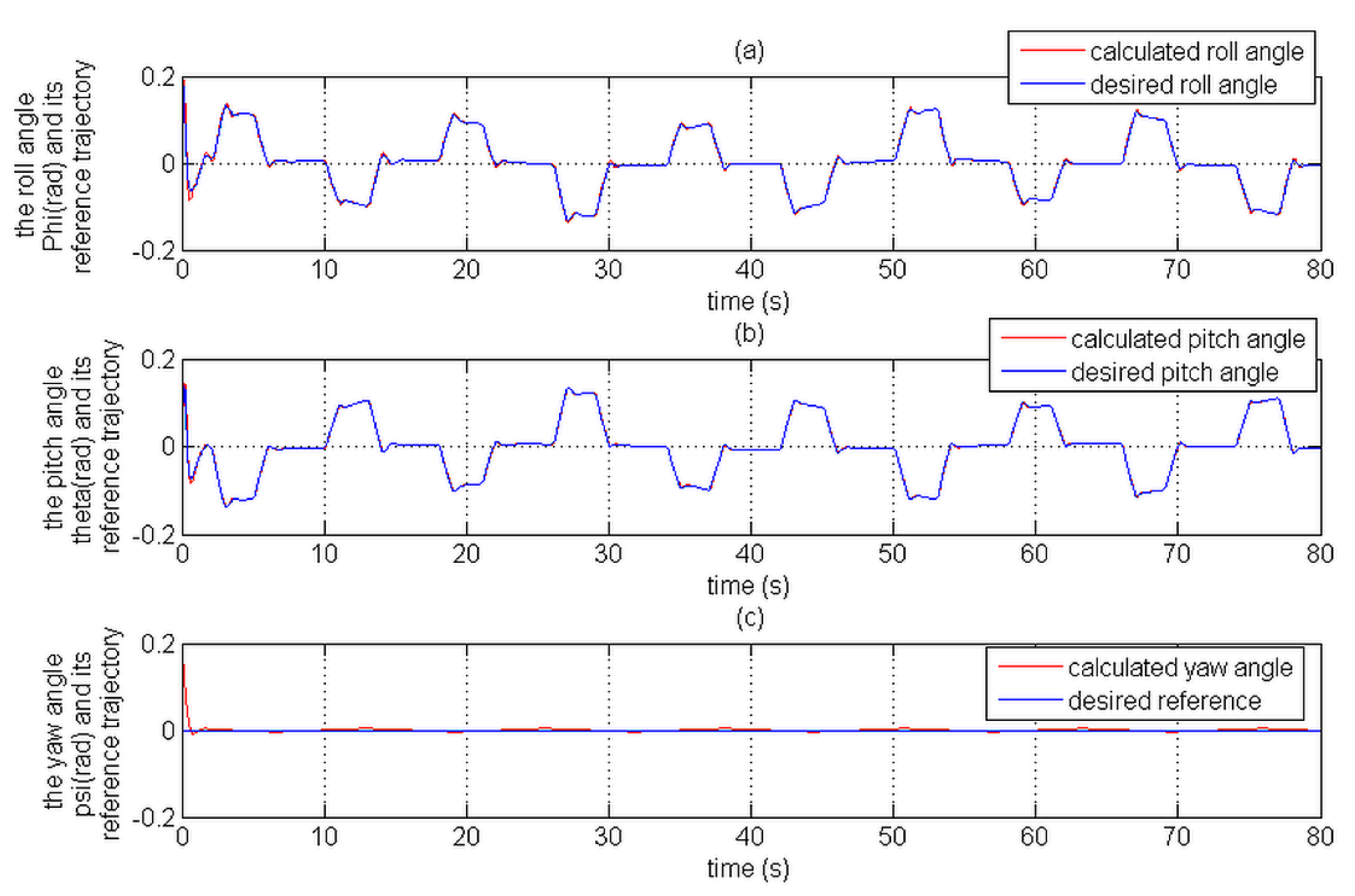
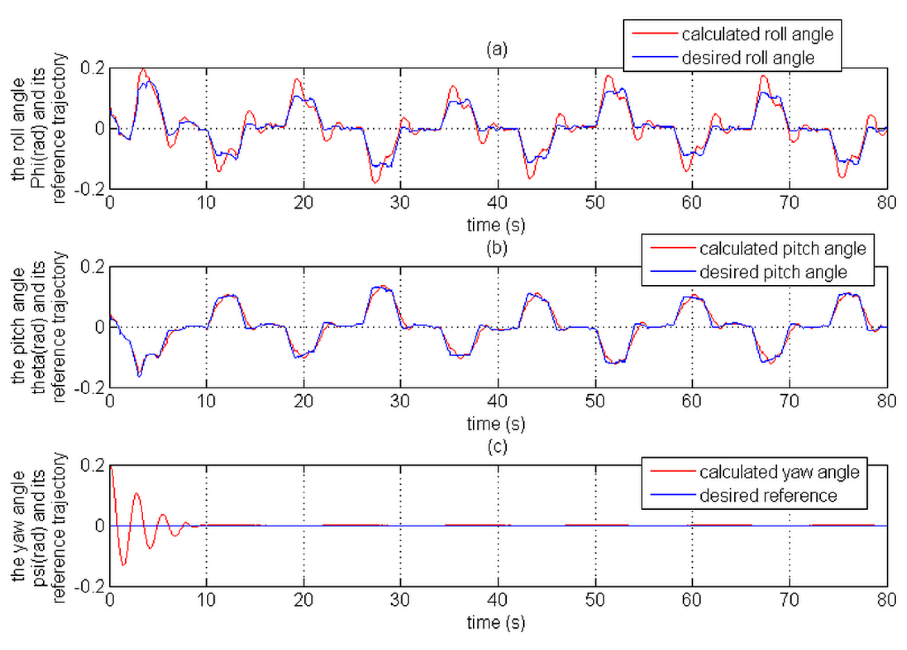
Figure 20 show the position tracking evolution and its reference trajectory; the evolution of the attitude tracking and its desired reference are shown in
Figure 21 and
Figure 22;
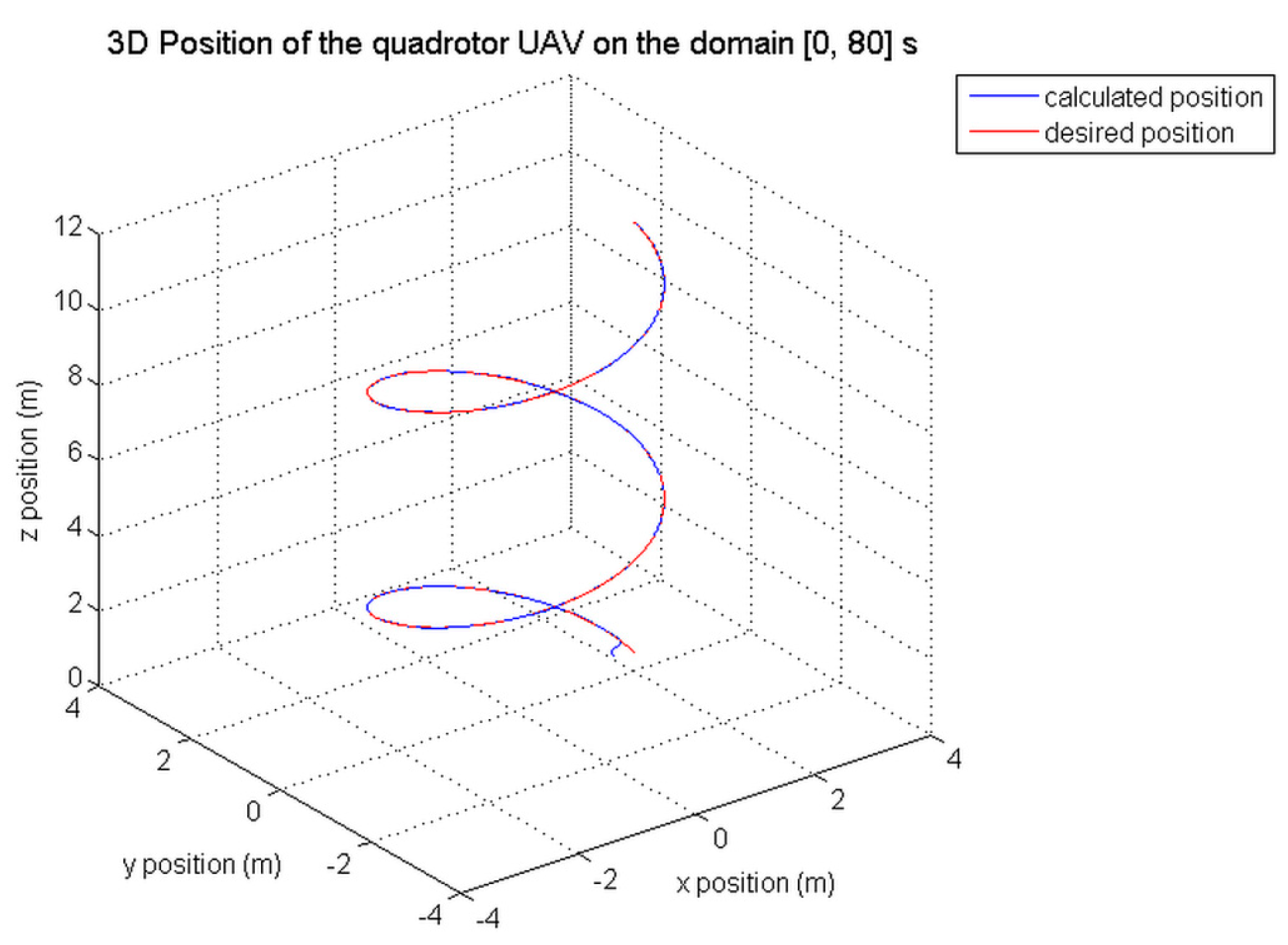
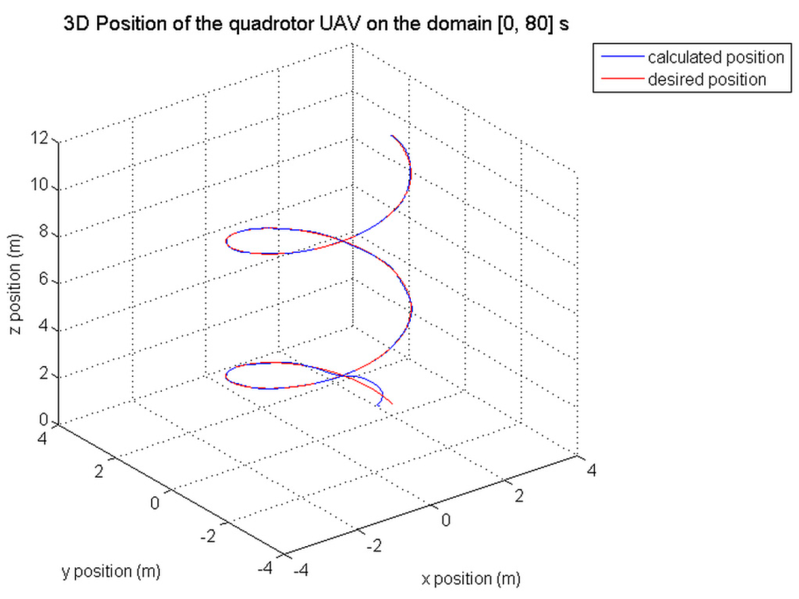
Figure 23,
Figure 24,
Figure 25 and
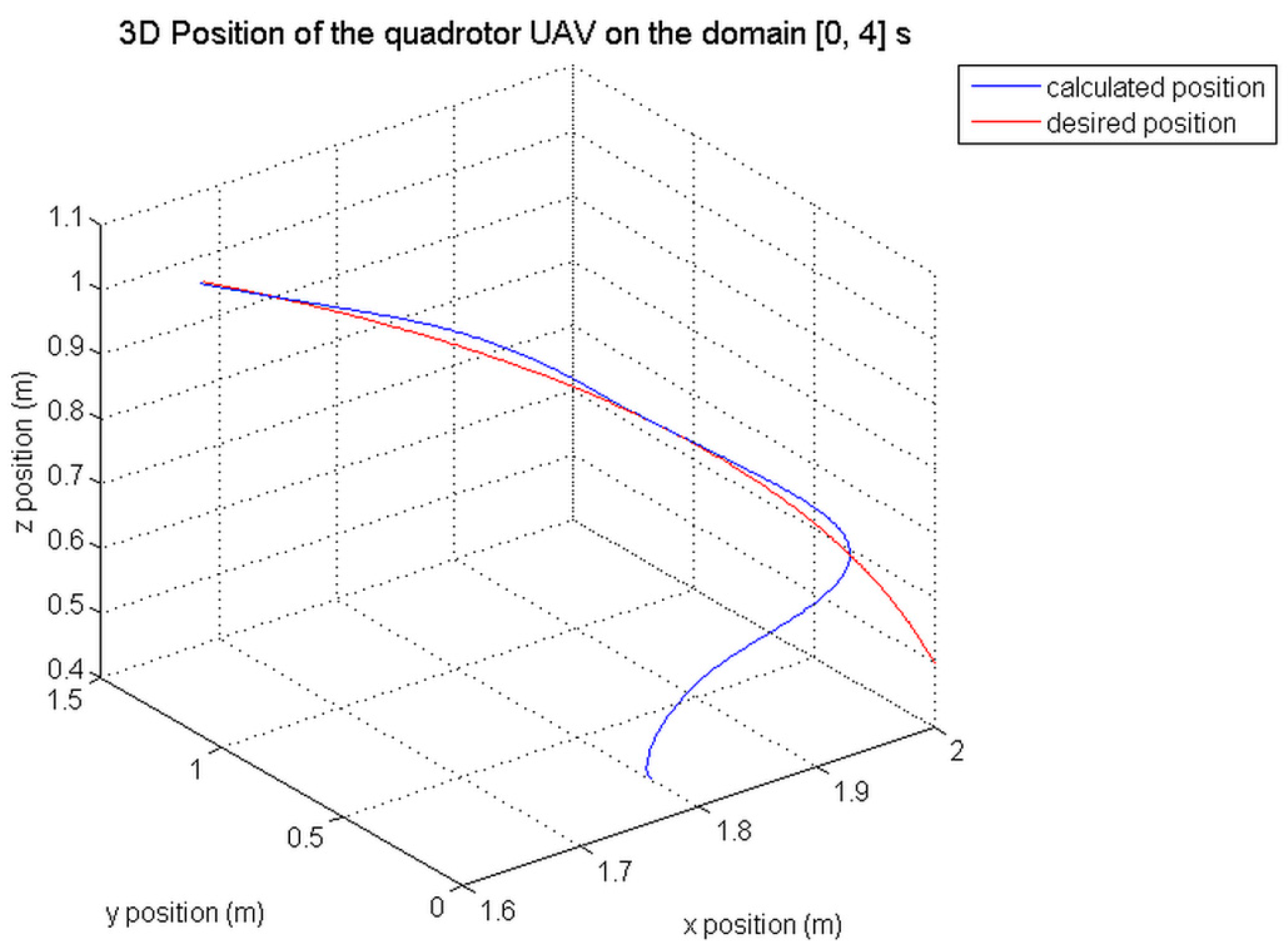
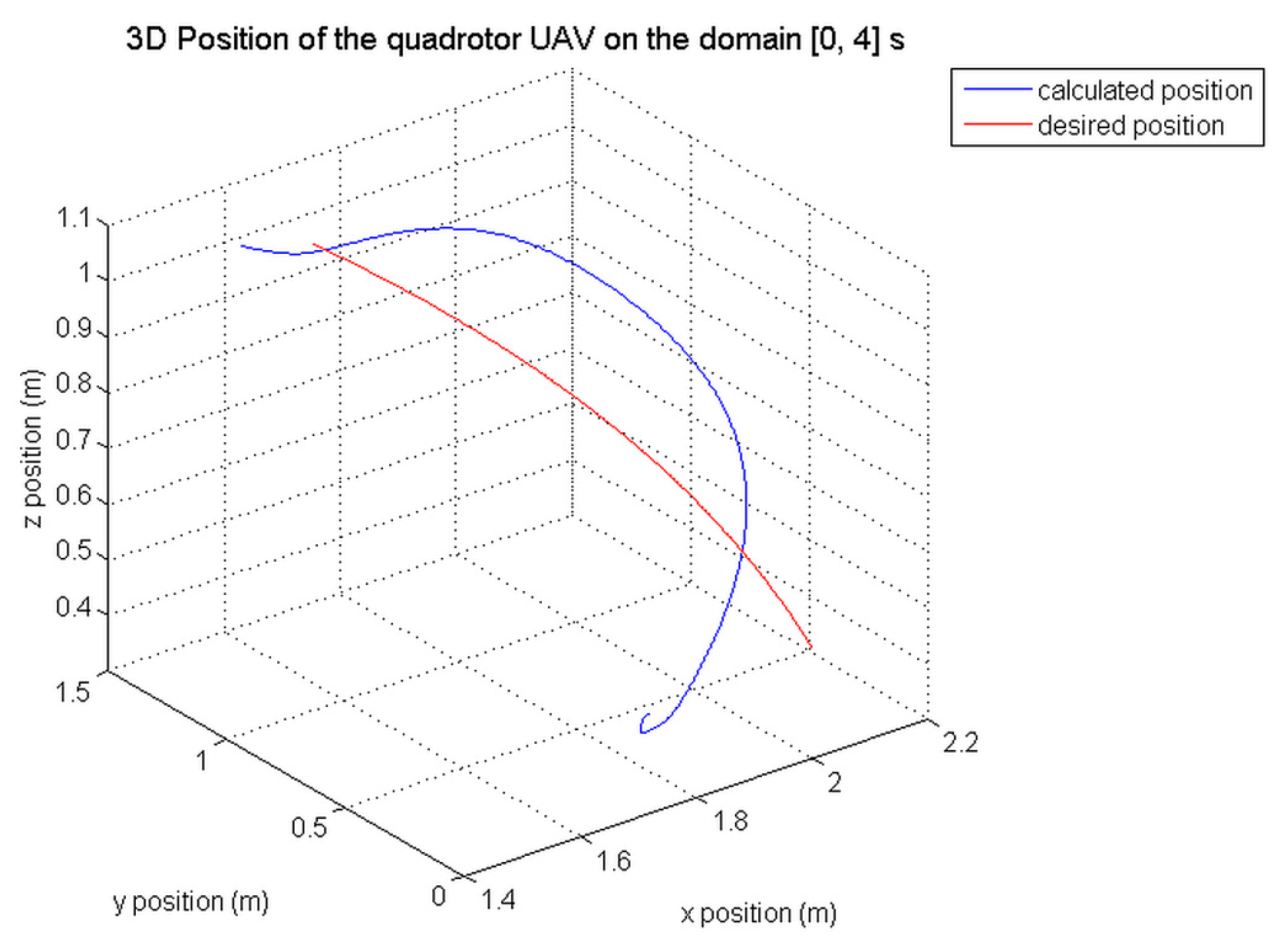
Figure 26 represent, for both tracking control methods, the 3D position of the quadrotor and its reference trajectory in the time intervals [0, 80] s and [0, 4] s; and finally,
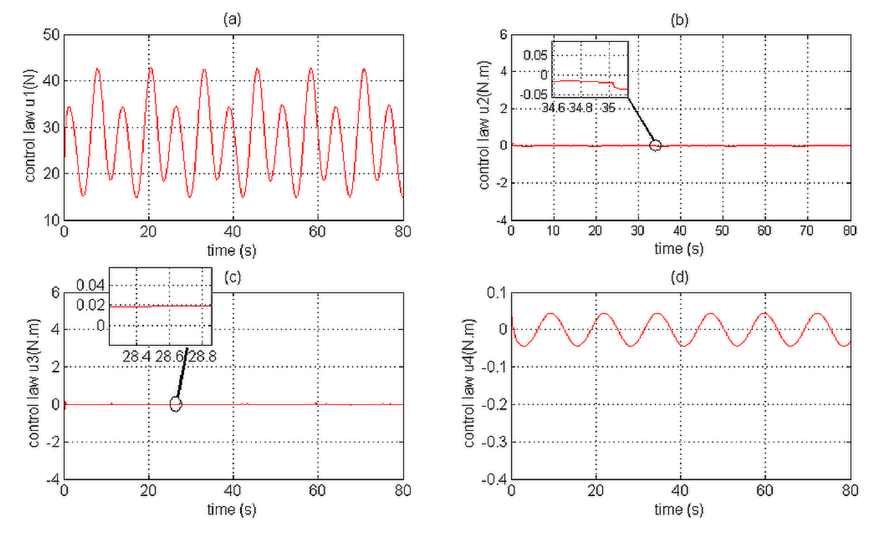
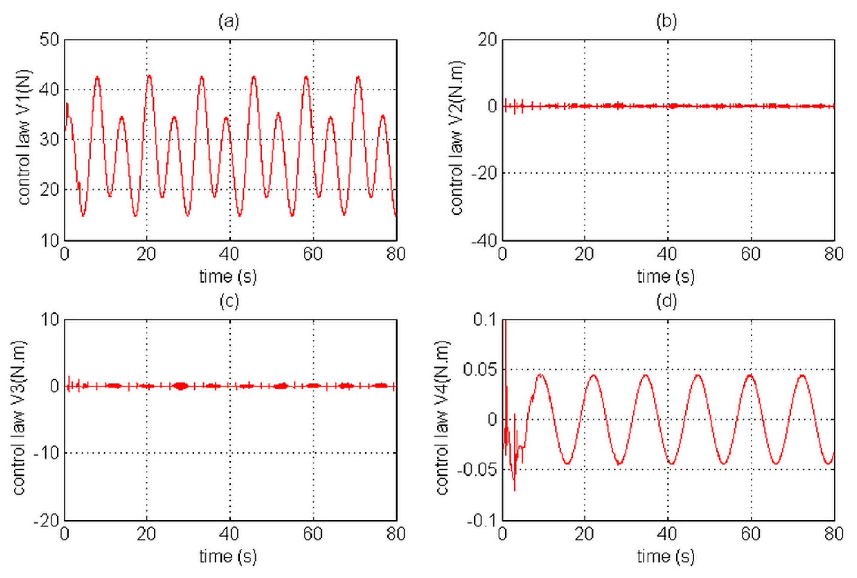
Figure 27 and
Figure 28 represent the position and the attitude control laws of the two compared approaches of tracking control.
In comparison with the CMTC, the PTCM shows the best tracking control performance. This superiority of the PTCM in ensuring the desired objective of control despite unknown dynamics, parameter variations, unknown disturbances, and unknown physical parameters of the studied quadrotor is due to both of its features, namely (1) optimal estimation of unknown dynamics, and (2) a great efficiency in rejecting all disturbances that influence the system robustness. Also, we noticed that the control laws of the PTCM are smooth and do not present any variations which is not the case for the CMTC. Thus, the undesired chattering phenomenon is avoided, and the tracking accuracy is preserved.
6. Conclusions
In this study, we developed a robust full tracking control design method for quadrotor UAVs with unknown dynamics and unknown physical parameters that are subject to unknown and unpredictable disturbances. In order to efficaciously estimate the unknown functions, seven IT2-AFSs and five adaptive systems were designed. Then, based on IT2-AFSs, an optimal IT2-AFRSMCL was added to the global control law in order to deal with the approximation errors and unknown and unpredictable disturbances that influence the quadrotor dynamics while simultaneously avoiding the chattering phenomenon. The underactuated problem of the quadrotor UAVs was resolved by introducing two virtual control inputs to the control system. A mathematical analysis showed that the proposed algorithm of control is stable in the sense of Lyapunov and can establish asymptotic convergence of the system state trajectories to desired references. The obtained results confirmed the mathematical analysis, ensuring the predetermined objective of control.


